A Projection Method to Solve Linear Systems

in Tensor Format

Jonas Ballani∗, and Lars Grasedyck†

Bericht Nr. 309 April 2010

Key words: Low rank, Tucker, hierarchical Tucker,

Kronecker–product matrix.

AMS subject classifications: 15A69, 90C06, 65F10

Institut fur Geometrie und Praktische Mathematik

RWTH Aachen

Templergraben 55, D–52056 Aachen (Germany)

∗Max Planck Insitute for Mathematics in the Sciences, Inselstr. 22–26, D–04109 Leipzig, Germany.

†Institut fur Geometrie und Praktische Mathematik, RWTH Aachen, Templergraben 55, 52056 Aachen.

Financial support from the DFG SPP–1324 under grant GRA2179/2–1 gratefully acknowledged.

A Projection Method to Solve Linear Systems

in Tensor Format

Jonas Ballani ∗, Lars Grasedyck †

April 30, 2010

In this paper we propose a method for the numerical solution of linear systemsof equations in low rank tensor format. Such systems may arise from the discreti-sation of PDEs in high dimensions but our method is not limited to this type ofapplication. We present an iterative scheme which is based on the projection of theresidual to a low dimensional subspace. The subspace is spanned by vectors in lowrank tensor format which — similarly to Krylov subspace methods — stem from thesubsequent (approximate) application of the given matrix to the residual. All cal-culations are performed in hierarchical Tucker format which allows for applicationsin high dimensions. The mode size dependency is treated by a multilevel method.We present numerical examples that include high-dimensional convection-diffusionequations and shift-invert eigenvalue solvers.

1 Introduction

This paper is concerned with the solution of linear systems

Ax = b (1)

where the system matrix A is given as the sum of d Kronecker products of matrices, i.e.

A =

kA∑

j=1

d⊗

µ=1

Aj,µ, (2)

and the right-hand side b is given as a tensor of low (canonical) rank. A matrix of the form (2)is said to be given in Kronecker format. Every solution strategy which considers A as a full andunstructured matrix will result in a computational complexity that grows exponentially in dand is therefore intractable for d ≫ 2. If x can be approximated by a vector of low tensor rank,solution strategies which exploit the tensor structure of the linear system become applicable.We will propose a projection method with a complexity of O(dkA) which can be applied evenin high dimensions.

∗Max Planck Institute for Mathematics in the Sciences, Inselstraße 22–26, D-04109 Leipzig, Germany†Institut fur Geometrie und Praktische Mathematik, RWTH Aachen, Templergraben 55, D-52056 Aachen,

Germany. Financial support from the DFG SPP-1324 under grant GRA2179/2-1 gratefully acknowledged.

1

1.1 PDEs in High Dimension

As an example where a linear system (1) with A given in Kronecker format may arise, weconsider the partial differential equation

−∆u = f in Ω := (0, 1)d, (3)

u = 0 on Γ := ∂Ω.

A finite difference discretisation of (3) leads to a linear system (1) where A is of the specialform

A =

d∑

j=1

In1⊗ · · · ⊗ Inj−1

⊗ Aj ⊗ Inj+1⊗ · · · ⊗ Ind

. (4)

Here, Aj ∈ Rnj×nj denotes the stiffness matrix of the 1d Laplacian and Inj

denotes the nj ×nj identity matrix. A similar structure arises for finite element discretisations and for otheroperators of the form div σ∇ + ∇ · b + c where a, b, c are constant.

In [8] we have shown that u has an integral representation which can be approximated byvectors of low rank. The approximation is based on the computation of integrals of matrixexponentials by a quadrature rule using sums of exponentials. The method scales linearly inthe dimension d and it is only applicable for definite systems of the form (4) (commutativity ofthe summands is required).

1.2 Related Solution Strategies

Beylkin and Mohlenkamp [3] reformulate (1) as a linear least squares problem. For a giventensor rank of x, they fix all but one direction and solve the associated normal equations.Alternating cyclically through all possible directions, the residual is decreased at each iterationstep. This procedure is commonly known as an alternating least squares (ALS) approach (cf.e.g. [2], [3]).

Espig, Hackbusch, Rohwedder, and Schneider [7] have proposed a direct minimisation of thefunctional

f(x) = ‖Ax − b‖2

where x is assumed to be of fixed rank. The computation of the gradient of f is performedwith respect to the low rank structure of x. This entails the existence of local minima that areno solutions of (1) which cannot be trivially avoided. To apply the method of [7], we thereforehave to rely on additional assumptions to avoid local minima.

Kressner and Tobler [15] have introduced a so-called tensor Krylov subspace method. Usingthe special structure of (4), they construct a tensorised Krylov space which is the tensor productof usual Krylov subspaces. The basis of the tensorised Krylov space can be used to transformthe original linear system to a system of smaller (mode) size. If the smaller system can be solvedefficiently, this approach leads to acceptable convergence rates for typical model problems. Asa major drawback, the computational complexity for the solution of the smaller system stillscales exponentially in d.

Krylov subspace methods for tensor computations have also been analysed by Elden andSavas [5] but not for the solution of linear systems in low rank tensor format.

1.3 Generalised Low Rank GMRES

In this article, we propose a new method for the solution of (1) which is derived from a typicalprojection method. In analogy to a GMRES method, we will construct a low dimensional

2

subspace spanned by tensors of low rank. The linear system projected onto this subspace issolved in each iteration step and the iterate is truncated to low rank. After this projection andtruncation step the process is restarted by the construction of a new subspace. The propertiesof our new method are:

• It has a complexity of O(dkA) and is therefore applicable in high dimensions

• Except the Kronecker format, no additional structure of the addends of A is needed, inparticular we do not require the form (4)

• The residual is non-increasing at each iteration step

• All calculations are performed in hierarchical Tucker format and rely on simple linearalgebra tools like the SVD for the truncation of tensors

The hierarchical Tucker format has been introduced by Hackbusch and Kuhn [14]. It allowsfor an efficient representation of tensors with linear complexity in d. Moreover, a truncationprocedure is available [9] which scales linearly in d and hence permits an approximate arithmeticin high dimensions. As a side-effect of our method, the capabilities of the approximate arithmeticin hierarchical Tucker format for the usage in iterative schemes can be demonstrated.

1.4 Iterate and Approximate

Hackbusch, Khoromskij and Tyrtyshnikov [13] analyse the convergence of a truncated iterationprocess of the form

xℓ+1 := T (Φℓ(xℓ)) (5)

where Φℓ is a one-step operator and T is some truncation operator. They show that if (5)converges for T = Id, then the process will also converge for small perturbations of the iteratesinduced by a general truncation operator T . Unfortunately, this concept will not directlyapply to our method as we will work with an operator that truncates tensors to a fixed rank.Alternatively, one could choose all involved ranks adaptively to guarantee a certain precision.As some numerical experiments show, this would lead to a successive growth in the ranks whichincreases the computing time significantly.

The rest of this article is organised as follows. In the second section, we introduce some basicdefinitions related to tensor decompositions. In the third section, we will derive our new solutionmethod for (1) from a general projection method. In order to make our setting more accessible,we will afterwards introduce the hierarchical Tucker format which allows for an efficient andaccurate representation of tensors. Moreover, an approximate arithmetic is defined which relieson the truncation of tensors in hierarchical Tucker format. In section five, we will adapt theprojection method in tensor format to the case of the hierarchical Tucker format. Afterwards,we will briefly discuss the acceleration of our method by multigrid methods and the applicationto eigenvalue problems. In the last section, we illustrate the potential of our method by somenumerical examples.

2 Basic Definitions

In this section, we introduce some basic definitions related to tensors that will be used through-out the whole article.

3

Notation 1 (Index set). Let d ∈ N and n1, . . . , nd ∈ N. We consider tensors as vectors overproduct index sets. For this purpose, we introduce the d-fold product index set

I := I1 × · · · × Id, Iµ := 1, . . . , nµ, µ ∈ 1, . . . , d.Definition 2 (Elementary tensor, order). A tensor X ∈ R

I is called an elementary tensor, ifit can be represented as the tensor product of vectors xµ ∈ R

nµ , µ ∈ 1, . . . , d, i.e.

X =

d⊗

µ=1

xµ. (6)

The entries of X are given by

X(i1,...,id) =

d∏

µ=1

(xµ)iµ , iµ ∈ Iµ.

Tensors of the form (6) are often called rank 1 tensors. The integer d is the order or dimension

of the tensor X.

Definition 3 (Tensor rank, k-term representation). The rank k of a tensor X ∈ RI is the

minimal number k ∈ N0 such that there exist elementary tensors X1, . . . ,Xk with

X = X1 + . . . + Xk =

k∑

j=1

d⊗

µ=1

xj,µ, xj,µ ∈ Rnµ . (7)

A tensor of the form (7) is said to be given in a k-term representation. In the literature, therepresentation (7) is sometimes referred to as PARAFAC (parallel factors), CANDECOMP

(canonical decomposition), (CP), or Kronecker format.

Definition 4 (Tucker rank, Tucker format). The Tucker rank of a tensor X ∈ RI is the tuple

(k1, . . . , kd) with minimal entries kµ ∈ N0 such that there exist orthonormal vectors uj,µ ∈ Rnµ

and a so-called core tensor C ∈ Rk1×...×kd with

X =

k1∑

j1=1

· · ·kd∑

jd=1

C(j1,...,jd)

d⊗

µ=1

ujµ,µ, 〈ui,µ, uj,µ〉 = δi,j . (8)

The representation of the form (8) is called the Tucker format.

Definition 5 (Matrix in Kronecker format). The Kronecker product for matrices Aµ ∈ Rnµ×nµ ,

µ ∈ 1, . . . , d, is defined by

d⊗

µ=1

Aµ

(i1,...,id),(j1,...,jd)

:=d∏

µ=1

(Aµ)iµ,jµ , iµ, jµ ∈ Iµ.

A matrix A of the form

A =

kA∑

j=1

d⊗

µ=1

Aj,µ, Aj,µ ∈ Rnµ×nµ , (9)

is said to be given in Kronecker format. The multiplication of a matrix A = ⊗dµ=1Aµ by a

vector x = ⊗dµ=1xµ reads

d⊗

µ=1

Aµ

d⊗

µ=1

xµ

=

d⊗

µ=1

(Aµxµ).

4

3 Projection Methods

3.1 A General Projection Method

Consider the linear systemAx = b

where A ∈ RI×I is a non-singular matrix and b ∈ R

I . Let x0 be an initial guess and let V, Wbe two m-dimensional subspaces of R

I . By means of a projection method, we try to find anapproximate solution x ∈ x0 + V such that the residual b − Ax is orthogonal to W. Given theinitial residual r0 = b−Ax0, the approximate solution can be defined as x = x0 + δ, δ ∈ V, suchthat

〈r0 − Aδ,w〉 = 0 for all w ∈ W.

Let Vm = [v1, . . . , vm] ∈ RI×m and Wm = [w1, . . . , wm] ∈ R

I×m be such that the column vectorsof Vm and Wm form a basis of V and W, respectively. If the approximate solution is written inthe form x = x0 + Vmy, y ∈ R

m, the orthogonality condition leads immediately to the followingsystem of equations

W⊤mAVmy = W⊤

mr0.

If the matrix W⊤mAVm is non-singular, the approximate solution is uniquely defined. In par-

ticular, W⊤mAVm is non-singular if A is non-singular and W = AV (cf. [17] Prop. 5.1). If

W = AV where V is the m-th Krylov subspace, i.e. V = spanr0, Ar0, A2r0, . . . , A

m−1r0, theprojection method is known as GMRES. The projection algorithm is summarised in Algorithm1. Note that we have assumed a fixed dimension m of the space V. In a GMRES method, thisparameter is usually chosen dynamically as the residual can be estimated cheaply in the innerloop when the column vectors of Vm are orthonormal. Later on, we will not be able to rely onorthonormality.

Algorithm 1 Projection method (GMRES)

choose x0

for ℓ = 0, 1, . . . do

rℓ := b − Axℓ

if ‖rℓ‖ / ‖b‖ < ε then

return xℓ

end if

v1 := rℓ/ ‖rℓ‖for j = 1, . . . ,m do

wj := Avj

solve (V ⊤j Vj)α = V ⊤

j wj

vj+1 := wj −∑j

i=1 αivi

vj+1 := vj+1/ ‖vj+1‖end for

solve (W⊤mAVm)y = W⊤

mrℓ

xℓ+1 := xℓ + Vmyend for

5

3.2 A Projection Method in Tensor Format

Let us assume that the matrix A ∈ RI×I is given in Kronecker format, i.e.

A =

kA∑

j=1

d⊗

µ=1

Aj,µ, Aj,µ ∈ Rnµ×nµ ,

and that the right-hand side possesses the representation

b =

kb∑

j=1

d⊗

µ=1

bj,µ, bj,µ ∈ Rnµ .

Every naive strategy which aims at solving (1) will have a complexity that scales exponentiallyin d and will be prohibitively expensive. We therefore want to introduce a new method whichis inspired by the general projection method that completely relies on calculations with tensorsof low rank. This will effectively reduce the complexity to O(dkA) which allows us to solvesystems in high dimensions.

In analogy to the general projection method, we will generate a sequence of iteratesxℓl∈N, xℓ ∈ R

I , in tensor format of low rank such that the norm of the residual does notincrease at each iteration step. To this end, assume that xℓ ∈ R

I is given in low rank formatand let rℓ := b − Axℓ. We first construct a subspace V = spanv1, . . . , vm ⊂ R

I such that allbasis vectors vj are given in low rank format. Define the first basis vector by

v1 := T (rℓ), v1 := v1/ ‖v1‖ ,

where T : RI → R

I is some truncation operator that truncates a tensor either to a fixedrank or to a given accuracy. Now let v1, . . . , vj ∈ R

I be given in low rank format and letVj := [v1, . . . , vj ] ∈ R

I×j. As in a Krylov subspace method, define wj := Avj and solve(V ⊤

j Vj)α = V ⊤j wj. A new basis vector is now defined by

vj+1 := T(

wj −j∑

i=1

αivi

)

, vj+1 := vj+1/ ‖vj+1‖ .

Note that, due to the truncation, the columns of Vm are no longer orthogonal. Moreover, thesubspace V = spanv1, . . . , vm is not a Krylov subspace. Nonetheless, the affine space xℓ+V willcontain an element which does not increase the norm of the residual. Let zℓ+1 := xℓ +Vmy, y ∈R

m. To perform the projection of the new residual b − Azℓ+1 onto W = spanw1, . . . , wm, letWm := [w1, . . . , wm] ∈ R

I×m and solve (W⊤mAVm)y = W⊤

mrℓ. The new iterate is now defined by

zℓ+1 = xℓ + Vmy, xℓ+1 := T (zℓ+1).

For the exact residual b − Azℓ+1, we have

‖b − Azℓ+1‖ ≤ ‖rℓ‖

because of the projection of the residual onto W. To ensure the convergence of the projectionmethod, the truncation xℓ+1 = T (zℓ+1) has to be done in such a way that the norm of theresidual rℓ+1 = b − Axℓ+1 is not increased, i.e.

xℓ+1 = T (zℓ+1) s.t. ‖rℓ+1‖ ≤ ‖rℓ‖ .

6

Algorithm 2 Projection method in tensor format

1: choose x0

2: for ℓ = 0, 1, . . . do

3: rℓ := b − Axℓ

4: if ‖rℓ‖ / ‖b‖ < ε then

5: return xℓ

6: end if

7: v1 := T (rℓ)8: v1 := v1/ ‖v1‖9: for j = 1, . . . ,m do

10: wj := Avj

11: solve (V ⊤j Vj)α = V ⊤

j wj

12: vj+1 := T(

wj −∑j

i=1 αivi

)

13: vj+1 := vj+1/ ‖vj+1‖14: end for

15: solve (W⊤mAVm)y = W⊤

mrℓ

16: zℓ+1 := xℓ + Vmy17: xℓ+1 := T (zℓ+1) s.t. ‖b − Axℓ+1‖ ≤ ‖rℓ‖18: end for

The algorithm is summarised in Algorithm 2.We have still left open which low rank format we want to use for the representation of vectors

in RI and, in particular, how the truncation operator T shall look like. Assume for a moment

that all vectors in Algorithm 2 were represented as rank k tensors. Each operation that requiresthe addition of two rank k tensors will result in a tensor of rank 2k. Hence, the truncationof a rank 2k tensor to rank k is necessary if we do not want to increase the rank at eachiteration step. A typical way to perform the truncation is to apply an alternating least squares(ALS) approach which – in most cases – converges rather slowly. An efficient algorithm forthe truncation has been proposed by Espig [6] which is based on Newton-like techniques. Bothalgorithms are local optimisation procedures which crucially depend on the choice of initialvalues. Unfortunately, up to now there are no known algorithms which guarantee an a priorierror bound for the truncation.

Consider on the other hand the representation of tensors in Tucker format. Here, reliabletruncation procedures like the higher order SVD and a priori error bounds are available [16].The major drawback of this format is its exponential complexity in d for the storage of the coretensor and thus for all relevant arithmetic operations. For low dimensions where d ≤ 6, thismight not be a problem and Algorithm 2 can be adapted to this case but for high dimensionswith d > 6 we need something else.

In the following section we will present the so-called hierarchical Tucker format introduced byHackbusch and Kuhn [14] which addresses the above mentioned problems. The format providesboth a representation of tensors and reliable truncation procedures with linear complexity ind. Therefore the hierarchical Tucker format is an efficient means for performing arithmeticoperations with tensors without sacrificing the low rank structure. Hence, it is exactly what weneed for our projection method in tensor format.

7

4 The Hierarchical Tucker Format

For the definition of the hierarchical Tucker format, we adopt the notation from [9].

Definition 6 (Dimension tree). A dimension tree TI for a dimension d ∈ N is a tree with rootRoot(TI) = 1, . . . , d and depth p = ⌈log2(d)⌉ := mini ∈ N0 | i ≥ log2(d) such that eachnode t ∈ TI is either

1. a leaf and singleton t = µ on level ℓ ∈ p − 1, p or

2. the disjoint union of two successors S(t) = s1, s2,t = s1∪s2.

The level ℓ of the tree is defined as the set of all nodes having a distance of exactly ℓ to theroot. The set of leaves of the tree is denoted by L(TI) and the set of interior (non-leaf) nodesis denoted by J (TI). A node of the tree is a so-called mode cluster (a union of modes). Thecanonical dimension tree is a dimension tree where each node t = µ1, . . . , µq, q > 1, has twosuccessors

t1 = µ1, . . . , µr, t2 = µr+1, . . . , µq, r := ⌊q/2⌋ := maxi ∈ N0 | i ≤ q/2.Definition 7 (Matricisation). For a mode cluster t in a dimension tree TI we define the com-plementary cluster t′ := 1, . . . , d \ t,

It :=×µ∈t

Iµ, It′ :=×µ∈t′

Iµ,

and the corresponding t-matricisation

Mt : RI 7→ R

It×It′ , (Mt(A))(iµ)µ∈t,(iµ)µ∈t′:= A(i1,...,id).

We use the short notation A(t) := Mt(A).

Definition 8 (Hierarchical rank). Let TI be a dimension tree. The hierarchical rank (kt)t∈TI

of a tensor A ∈ RI is defined by

∀t ∈ TI : kt := rank(A(t)).

The set of all tensors of hierarchical rank (node-wise) at most (kt)t∈TIis denoted by

H-Tucker((kt)t∈TI) := A ∈ R

I | ∀t ∈ TI : rank(A(t)) ≤ kt.Definition 9 (Frame tree, t-frame, transfer tensor). Let t ∈ TI be a mode cluster and (kt)t∈TI

a family of non-negative integers. We call a matrix Ut ∈ RIt×kt a t-frame and the tuple (Us)s∈TI

of frames a frame tree. A frame is called orthogonal if its columns are orthonormal. A frametree is called orthogonal if each non-root frame is. A frame tree is nested if for each interiormode cluster t with successor S(t) = t1, t2 the following relations holds:

span(Ut)i | 1 ≤ i ≤ kt ⊂ span(Ut1)i ⊗ (Ut2)j | 1 ≤ i ≤ kt1 , 1 ≤ i ≤ kt2.The corresponding tensor Bt ∈ R

kt×kt1×kt2 of coefficients for the representation of the columns(Ut)i of Ut by the columns of Ut1 and Ut2 ,

(Ut)i =

kt1∑

j=1

kt2∑

l=1

(Bt)i,j,l(Ut1)j ⊗ (Ut2)l,

is called the transfer tensor.

8

For a nested frame tree it is sufficient to provide the transfer tensors Bt for all interior modeclusters t ∈ J (TI) and the t-frames Ut for the leaves t ∈ L(TI). Note that we have not yetimposed an orthogonality condition on the t-frames.

Definition 10 (Hierarchical Tucker format). Let TI be a dimension tree, (kt)t∈TIa family of

non-negative integers and A ∈ H-Tucker((kt)t∈TI). Let (Ut)t∈TI

be a nested frame tree withtransfer tensors (Bt)t∈J (TI) and

∀t ∈ TI : image(A(t)) = image(Ut), A = U1,...,d.

Then the representation ((Bt)t∈J (TI), (Ut)t∈L(TI)) is a hierarchical Tucker representation of A.The family (kt)t∈TI

is the hierarchical representation rank. Note that the columns of Ut neednot be linear independent.

Definition 11 (Orthogonal frame projection). Let TI be a dimension tree, t ∈ TI and Ut anorthogonal t-frame. We define the orthogonal frame projection πt : R

I 7→ RI in matricised form

by(πtA)(t) := UtU

⊤t A(t).

Theorem 12 (Hierarchical truncation error, [9] Theorem 17 and Remark 18). Let TI be a

dimension tree and A ∈ RI . Let Abest denote the best approximation of A in H-Tucker((kt)t∈TI

)and let πt be the orthogonal frame projection for the t-frame Ut that consists of the left singular

vectors of At corresponding to the kt largest singular values σt,i of A(t). Then for any order of

the projections πt, t ∈ TI, holds∥

∥

∥

∥

∥

∥

A −∏

t∈TI

πtA

∥

∥

∥

∥

∥

∥

≤√

∑

t∈TI

∑

i>kt

σ2t,i ≤

√2d − 3

∥

∥

∥A − Abest∥

∥

∥ .

Theorem 13 (Characterisation of hierarchical approximability, [9] Theorem 24). Let TI be a

dimension tree, A ∈ RI , (kt)t∈TI

a family of non-negative integers and ε > 0. If there exists a

tensor Abest of hierarchical rank (kt)t∈TIand

∥

∥A − Abest∥

∥ ≤ ε, then the singular values of A(t)

for each node t can be estimated by√

∑

i>kt

σ2i ≤ ε.

On the other hand, if the singular values fulfil the bound√

∑

i>ktσ2

i ≤ ε/√

2d − 3, then the

truncation yields an H-Tucker tensor AH :=∏

t∈TIπtA such that

‖A − AH‖ ≤ ε.

This means that we can truncate a tensor A ∈ RI either to a given hierarchical rank (kt)t∈TI

,or we can prescribe node-wise tolerances ε/

√2d − 2 to obtain a guaranteed error bound of

‖A − AH‖ ≤ ε. As we are especially interested in calculations of fixed rank, we will introducea truncation operator that bounds the node-wise ranks by a constant.

Definition 14 (Truncation operator). Let k ∈ N and TI a dimension tree. For A ∈ RI we

introduce the truncation operator Tk : RI → R

I defined by

Tk(A) :=∏

t∈TI

πtA, (10)

where for t ∈ TI the columns of the frame Ut ∈ RIt×k are the first k left singular vectors of A(t).

9

If a tensor is already given in hierarchical Tucker format, A ∈ H-Tucker((kt)t∈TI), then the

truncation can be performed in a complexity of

O

dmaxt∈TI

k4t +

d∑

µ=1

nµk2µ

.

The hierarchical Tucker format provides a favourable setting for common arithmetic oper-ations like addition and multiplication of tensors and the matrix-vector product. Since theyfollow directly from the definition of the hierarchical Tucker format, the following three lemmasare given without proof.

Lemma 15 (Addition). Let TI be a dimension tree and A ∈ H-Tucker((kt)t∈TI), A′ ∈

H-Tucker((k′t)t∈TI

). Moreover, let ((Bt)t∈J (TI), (Ut)t∈L(TI )) and ((B′t)t∈J (TI), (U

′t)t∈L(TI )) be

hierarchical Tucker representations of A and A′, respectively. Define a family of non-negative

integers (k′′t )t∈TI

by

∀t ∈ TI \ Root(TI) : k′′t := kt + k′

t,

and k′′1,...,d := 1, the t-frames

∀t ∈ L(TI) : U ′′t := [Ut | U ′

t],

and the transfer tensors

∀t ∈ J (TI) \ Root(TI) : B′′t ∈ R

k′′t ×k′′

t1×k′′

t2

where t = t1∪t2 and

(B′′t )i,j,l :=

(Bt)i,j,l, 1 ≤ i ≤ kt, 1 ≤ j ≤ kt1 , 1 ≤ l ≤ kt2 ,

(B′t)i−kt,j−kt1 ,l−kt2

, 1 ≤ i − kt ≤ k′t, 1 ≤ j − kt1 ≤ k′

t1, 1 ≤ l − kt2 ≤ k′

t2,

0, otherwise,

and B′′1,...,d ∈ R

1×k′′t1×k′′

t2 where 1, . . . , d = t1∪t2 and

(B′′1,...,d)1,j,l :=

(B1,...,d)1,j,l, 1 ≤ j ≤ kt1 , 1 ≤ l ≤ kt2 ,

(B′1,...,d)1,j−kt1 ,l−kt2

, 1 ≤ j − kt1 ≤ k′t1

, 1 ≤ l − kt2 ≤ k′t2

,

0, otherwise .

Then ((B′′t )t∈J (TI), (U

′′t )t∈L(TI )) is a hierarchical Tucker representation of A′′ := A + A′.

Lemma 16 (Scalar multiplication). Let TI be a dimension tree and A ∈ H-Tucker((kt)t∈TI)

with hierarchical Tucker representation ((Bt)t∈J (TI), (Ut)t∈L(TI )). For c ∈ R define B′1,...,d :=

cB1,...,d and for all other t ∈ J (TI) \ Root(TI) let B′t := Bt. Then ((B′

t)t∈J (TI), (Ut)t∈L(TI ))is a hierarchical Tucker representation of A′ := cA.

Lemma 17 (Matrix-vector multiplication). Let TI be a dimension tree and A ∈H-Tucker((kt)t∈TI

) with hierarchical Tucker representation ((Bt)t∈J (TI), (Ut)t∈L(TI )). Let M ∈RI×I be a matrix given by

M =

d⊗

µ=1

Mµ, Mµ ∈ Rnµ×nµ .

For all t = µ ∈ L(TI) define

U ′t := MµUt.

Then ((Bt)t∈J (TI), (U′t)t∈L(TI)) is a hierarchical Tucker representation of A′ := MA.

10

It is straight-forward to see that the multiplication has a complexity of O(∑d

µ=1 n2µkµ) if the

Mµ are unstructured and O(∑d

µ=1 nµkµ) if the Mµ are sparse (i.e. allow for a matrix-vectormultiplication in O(nµ)).

Remark 18 (Norm, scalar product). In [9] we have shown how to compute the Euclidean norm

of a tensor in hierarchical Tucker format in O(

dmaxt∈TIk4

t +∑d

µ=1 nµk2µ

)

. The scalar product

of two vectors v,w ∈ H-Tucker((kt)t∈TI) may then be calculated via the elementary formula

〈v,w〉 =1

2

(

‖v + w‖2 − ‖v‖2 − ‖w‖2)

.

5 A Projection Method in Hierarchical Tucker Format

In this section, we adapt the projection method in tensor format to the setting of the hierarchicalTucker format. For this purpose, we will follow the algorithmic concept introduced in Section3.2. The basic idea is to construct a low-dimensional subspace which is spanned by vectors of lowrank in hierarchical Tucker format. Let us assume that xℓ, b ∈ H-Tucker((kt)t∈TI

). According tothe arithmetic operations introduced in the last section, we may calculate rℓ = b−Axℓ directlyin hierarchical Tucker format. We now can use the residual to construct a low-dimensionalsubspace of vectors of low rank. To keep computations as cheap as possible, we will bound thenode-wise ranks of the vectors vj spanning the subspace by a constant kv ∈ N. In analogy toSection 3.2 we define

v1 := Tkv(rℓ), v1 := v1/ ‖v1‖ , (11)

where we have specified the truncation operator to be of the form (10). Now let v1, . . . , vj ∈H-Tucker((kt)t∈TI

) be given such that kt ≤ kv for all t ∈ TI . Define Vj := [v1, . . . , vj ] ∈ RI×j

and let wj := Avj . For the definition of a new basis vector, we have to solve the system(V ⊤

j Vj)α = V ⊤j wj . The calculation of the entries of the matrix V ⊤

j Vj and of the vector V ⊤j wj

merely requires the evaluation of scalar products which can easily be done according to Remark18. A new basis vector is now defined by

vj+1 := Tkv

(

wj −j∑

i=1

αivi

)

, vj+1 := vj+1/ ‖vj+1‖ .

The projection of the residual onto the subspace W spanned by the columns of Wm =[w1, . . . , wm] requires the solution of (W⊤

mAVm)y = W⊤mr0. Again, the matrix W⊤

mAVm andthe vector W⊤

mr0 may be calculated by the evaluation of scalar products of tensors in hierarchi-cal Tucker format.

Until now, we do not know whether the subspace V spanned by the columns of Vm was ”good”enough to lead to a sufficient decrease in the residual. What we expect is that for increasingvalues of kv, V attains similar properties as the exact Krylov subspace. To control the decreaseof the residual, we introduce a parameter ρ ∈ (0, 1) which is assumed to be small. If the newresidual rℓ −

∑mi=1 yiwi fulfils

∥

∥

∥

∥

∥

rℓ −m∑

i=1

yiwi

∥

∥

∥

∥

∥

< (1 − ρ) ‖rℓ‖ , (12)

we have chosen a subspace V that guarantees a decrease of the residual with rate 1 − ρ. If(12) is not fulfilled, we have to modify the subspace V such that it contains an element which

11

decreases the residual faster. We strongly expect that this is the case if we approximate theexact Krylov space better. Therefore, we increase kv and construct a new set of basis vectorsby starting at (11) where we substitute the truncation operator Tkv by Tkv+1.

Assume now that (12) is fulfilled. Formally, the new iterate may be written as zℓ+1 :=xℓ +Vmy. As the addition of tensors increases the rank, we also would like to apply a truncationoperator to the new iterate. In a similar way as before, we may truncate zℓ+1 by Tkx wherekx ∈ N is chosen such that the convergence is preserved. This means that we have to require

‖b − Axℓ+1‖ < ‖rℓ‖ (13)

where xℓ+1 := Tkx(zℓ+1). By subsequently increasing kx, we can find a value such that (13) isfulfilled since for the exact iterate zℓ+1 we can rely on the bound (12). Thus we have arrived ata new iterate xℓ+1 which is again given in tensor format of low rank. We have summarised allsteps in Algorithm 3.

As the truncation of tensors in hierarchical Tucker format scales like O(k4) for the node-wiseranks, it is advantageous to keep all ranks as small as possible throughout the whole iterationprocess. At first, this may seem unnatural as for this purpose we have to choose a small value ofρ resulting in a slow convergence behaviour. But – as the numerical evidence shows – this policypays off, since we can perform a much higher number of iterations at the same computationalcosts.

Algorithm 3 Projection method in hierarchical Tucker format

choose x0 and ρ ∈ (0, 1)kv := 1, kx := 1for ℓ = 0, 1, . . . do

rℓ := b − Axℓ

if ‖rℓ‖ / ‖b‖ < ε then

return xℓ

end if

repeat

construct v1, . . . , vm with T := Tkv as in lines 7 to 14 of Algorithm 2solve (W⊤

mAVm)y = W⊤mrℓ

kv := kv + 1until ‖rℓ −

∑mi=1 yiwi‖ < (1 − ρ) ‖rℓ‖

zℓ+1 := xℓ + Vmyrepeat

xℓ+1 := Tkx(zℓ+1)kx := kx + 1

until ‖b − Axℓ+1‖ < ‖rℓ‖end for

6 Multigrid Acceleration

In the previous section we have considered the solution of a general linear system in Kroneckerform. Many problems of practical interest however, require the solution of a linear system (1)where the system matrix stems from the discretisation of a partial differential equation. Inthis case GMRES type methods can suffer from large mode sizes nµ and their convergence ratetends to 1 as nµ → ∞.

12

For elliptic problems of large scale, multigrid methods have become the method of choice dueto their fast convergence and linear scaling. A comprehensive introduction may be found in [11],and we summarise the necessary basic ingredients in the following. It will turn out that onecan use the multigrid method for iterates in low rank tensor format and achieve linear scalingin the mode size nµ as well as the order d of the tensor.

The main idea is to construct a hierarchy of grids (hence the name multigrid) which are usedto reduce different frequency components of the error. The basic ingredients of a multigridmethod for the solution of a linear system (1) are:

1. A hierarchy of discrete problems

Aℓxℓ = bℓ, Aℓ ∈ RNℓ×Nℓ , ℓ = 1, . . . , L,

where N1 < . . . < NL, NL = #I, such that the problem on the coarsest level ℓ = 1 maybe solved directly, two subsequent systems are strongly related, and the problem on thefinest level ℓ = L is the original problem with AL = A that has to be solved.

2. Prolongation and restriction operators

P ℓℓ−1 : R

Nℓ−1 → RNℓ , Rℓ−1

ℓ : RNℓ → R

Nℓ−1

which transfer a vector from a grid on level ℓ to a vector on the next finer or coarser gridon level ℓ + 1 or ℓ − 1.

3. A smoothing operatorxi+1

ℓ = Sℓ(xiℓ, bℓ), ℓ = 1, . . . , L

that reduces high frequency components of the error.

Consider as an example a one-dimensional domain Ω = (0, 1). A hierarchy of grids with equidis-tant nodes may be defined by Ωℓ := i/2ℓ | 1 ≤ i < 2ℓ. A typical choice of the prolongationand restriction operator is then given by the corresponding matrices

P ℓℓ−1 =

1

2

121 1

21 1

. . .

, Rℓ−1ℓ =

1

4

1 2 11 2 1

. . .

.

The idea of a hierarchy of grids can be adapted to the multidimensional setting. Let Ω :=Ω1 × . . . × Ωd and let Ωµ,ℓ be a hierarchy of grids in mode-µ direction µ ∈ 1, . . . , d. Then

Ωℓ := Ω1,ℓ × . . . × Ωd,ℓ, ℓ = 1, . . . , L,

defines a hierarchy of grids for the domain Ω. Due to the product structure of the hierarchy ofgrids, the prolongation and restriction operators possess a nice tensor product structure. LetP ℓ

µ,ℓ−1 and Rℓ−1µ,ℓ be prolongation and restriction operators in mode-µ-direction µ ∈ 1, . . . , d,

respectively. Then

P ℓℓ−1 := P ℓ

1,ℓ−1 ⊗ . . . ⊗ P ℓd,ℓ−1, Rℓ

ℓ−1 := Rℓ−11,ℓ ⊗ . . . ⊗ Rℓ−1

d,ℓ ,

13

define prolongation and restriction operators for the hierarchy of grids Ωℓ.The smoothing operator Sℓ is not required to be a good solver, but it should remove high

frequency components of the error. A typical choice of Sℓ is a Jacobi or a Gauss-Seidel method.Here, for simplicity, we choose a Richardson method which is defined by

xi+1ℓ := xi

ℓ + ωℓ(bℓ − Aℓxiℓ)

where 0 < ωℓ < 2/(Aℓ) and (Aℓ) is the spectral radius of Aℓ.We still have to address how the linear systems on the coarsest level should be solved. For

the low-dimensional case, this is typically a small system which can be solved iteratively or bydirect methods. However, for high dimensions even the system on the coarsest level might betoo large. We therefore propose to use the projection method in hierarchical Tucker format tosolve this system. We have summarised the whole multigrid procedure in Algorithm 4.

Algorithm 4 xℓ = multigrid(ℓ, xℓ, bℓ)

if ℓ = 1 then

solve A1x1 = b1 by Algorithm 3return x1

else

for i = 1 to ν1 do

xℓ := xℓ + ωℓ(bℓ − Aℓxℓ)end for

dℓ−1 := Rℓ−1ℓ (bℓ − Aℓxℓ)

eℓ−1 := 0for i = 1 to γ do

eℓ−1 = multigrid(ℓ − 1, eℓ−1, dℓ−1)end for

xℓ := xℓ + P ℓℓ−1eℓ−1

for i = 1 to ν2 do

xℓ := xℓ + ωℓ(bℓ − Aℓxℓ)end for

return xℓ

end if

In practice it might be advisable not to use the multigrid method directly, but as a pre-conditioner in an iterative solver. For the iterative solver one can use again the GMRES-typeprojection method that we have presented here.

7 Application in an Eigenvalue Solver

We consider the problem to find eigenvalues and corresponding eigenvectors of large matrices,i.e. we seek a pair (λ, x) ∈ R × R

I \ 0 such that

Ax = λx.

In many applications, one specifically wants to find the smallest or the largest eigenvalue λmin orλmax for a given matrix, the eigenvectors corresponding to a few largest or smallest eigenvalues,or all eigenvectors corresponding to eigenvalues in a specific part of the complex plane. The

14

largest eigenvalue may be found by the well-known power method which only requires matrix-vector products. The smallest eigenvalue can be determined by the inverse power methodwhich relies on the subsequent solution of linear systems of the form Ax(ℓ+1) = y(ℓ) wherey(ℓ+1) := x(ℓ+1)/

∥

∥x(ℓ+1)∥

∥. The convergence of this iteration process may be controlled bymeans of the Rayleigh quotient ΛA(x) := 〈x,Ax〉/〈x, x〉. For an exact eigenpair (λ, x), wehave λ = ΛA(x). It is therefore a good strategy to use the Rayleigh quotient λ(ℓ) := ΛA(x(ℓ))to estimate an eigenvalue from its approximate eigenvector. The inverse power method maybe stopped if

∥

∥Ax(ℓ) − λ(ℓ)x(ℓ)∥

∥ < ε for some ε > 0. We have summarised the inverse powermethod in Algorithm 5.

Algorithm 5 Inverse power method

choose ε > 0 and y(1) ∈ RI with

∥

∥y(1)∥

∥ = 1for ℓ = 1, 2, . . . do

solve Ax(ℓ+1) = y(ℓ)

y(ℓ+1) := x(ℓ+1)/∥

∥x(ℓ+1)∥

∥

λ(ℓ+1) := ΛA(y(ℓ+1))if∥

∥Ay(ℓ+1) − λ(ℓ+1)y(ℓ+1)∥

∥ < ε then

return y(ℓ+1)

end if

end for

In general, any eigenvalue of A which is sufficiently separated from the rest of the spectrum,may be found by introducing a shift σ ∈ R which is assumed to be close to the sought eigenvalue.More precisely, let us assume that A has the eigenvalues λ1, . . . , λN and that

|σ − λi| < min|σ − λj| : 1 ≤ j ≤ N, j 6= i. (14)

If σ 6= λi, we have

Ax = λix ⇐⇒ (A − σI)−1x =1

λi − σx.

Hence, (A−σI)−1 has the same eigenvectors as A. Moreover, 1/(λi−σ) is the largest eigenvalueof (A− σI)−1 which can be found by the inverse power method. The application of the inversepower method to the shifted matrix A−σI is commonly known as a shift-invert strategy. Notethat if A is given in Kronecker format, also the matrix A − σI possesses this structure as theidentity may be written as I = I1 ⊗ . . .⊗ Id. In this case, the linear system in Algorithm 5 maytherefore be solved by the projection method in hierarchical Tucker format.

For eigenvalue problems of large scale it might not be advisable to apply the shift-invertstrategy directly since the involved solution of a linear system by a GMRES-type method maysuffer from a slow convergence rate. In analogy to the solution of linear systems of large scale,elliptic eigenvalue problems may efficiently be treated using a multigrid method [10]. A detailedanalyses of this multigrid eigenvalue scheme has been given in [1]. As in the usual multigridmethod, the eigenvalue problem has only to be solved on the coarsest level. The eigenvectors onthe finer levels result from the application of prolongation, restriction and smoothing operators.This setting can easily be adapted to the multi-dimensional case where we propose to use theprojection method in hierarchical Tucker format as a solver on the coarsest level. This allowsus to treat elliptic eigenvalue problems of large scale in high dimensions.

15

8 Numerical Examples

The following numerical examples shall illustrate the potential of the projection method for thesolution of linear systems in high dimensions. We are specifically interested in the followingquestions:

• Does the method converge sufficiently fast for all dimensions d?

• Does the hierarchical rank of x only increase moderately throughout the iteration process?

• Can we combine large dimensions d with a large mode size nµ?

Fortunately, we can answer all questions in the affirmative, at least for the range of examplesthat we consider. For simplicity, let now n := n1 = . . . = nd. In all examples, the dimension mof the subspace V is bounded by m = 10 but it may also be smaller when the basis vectors ofV become linearly dependent. The parameter ρ introduced in (12) has a strong impact on boththe convergence rate of the method and on the hierarchical ranks of the basis vectors spanningV. The higher the value of ρ, the higher is the convergence rate of the method implying a lownumber of iteration steps. On the other hand, a higher value of ρ leads to higher ranks for thebasis vectors spanning V which implies a much longer time for the truncation of vectors. Thechoice of ρ is therefore a trade-off and we are not aware of an optimal value. As a conservativechoice which works well in all examples we have set ρ := 10−4.

Example 19 (Symmetric case, [8]). As a symmetric example, we consider the Poisson equationin d dimensions, i.e.

−∆u = f in Ω = (0, 1)d,

u = 0 on Γ := ∂Ω.

A finite difference discretisation with mesh-width h leads to a linear system Ax = b where A isof the form (4) with

Aµ =1

h2

2 −1−1 2 −1

. . .. . .

. . .

−1 2 −1−1 2

.

Let the right-hand side be given such that it corresponds to the solution u =∏d

µ=1(xµ−x2µ). We

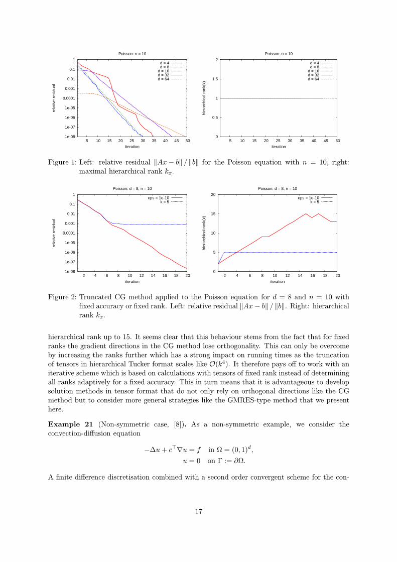
now fix the value of n := 10 and check the convergence of the projection method for dimensionsd = 4, 8, 16, 32, 64. The decrease of the relative residual ‖Ax − b‖ / ‖b‖ is shown in Fig. 1.Remarkably, the maximal hierarchical rank kx remains bounded by 1 throughout the wholesolution process.

Example 20 (Comparison to CG method). In the symmetric case, it is also possible to im-plement a conjugate gradient method that completely relies on truncated calculations in hier-archical Tucker format. To investigate this method, we made two experiments. First, we fixedε = 10−10 and truncated all vectors in the CG method with an accuracy of ε where all node-wiseranks were determined adaptively. Second, we fixed an upper bound on the hierarchical rankkx = 5 and compared both cases for d = 8 and n = 10 in Example 19. In both experiments thedecrease of the residual is similar up to an accuracy of 10−3 (cf. Fig. 2) but then the sequenceof iterates with fixed rank stagnates. The convergence can only be maintained by increasing the

16

1e-08

1e-07

1e-06

1e-05

0.0001

0.001

0.01

0.1

1

5 10 15 20 25 30 35 40 45 50

rela

tive

resi

dual

iteration

Poisson: n = 10

d = 4d = 8

d = 16d = 32d = 64

0

0.5

1

1.5

2

5 10 15 20 25 30 35 40 45 50

hier

arch

ical

ran

k(x)

iteration

Poisson: n = 10

d = 4d = 8

d = 16d = 32d = 64

Figure 1: Left: relative residual ‖Ax − b‖ / ‖b‖ for the Poisson equation with n = 10, right:maximal hierarchical rank kx.

1e-08

1e-07

1e-06

1e-05

0.0001

0.001

0.01

0.1

1

2 4 6 8 10 12 14 16 18 20

rela

tive

resi

dual

iteration

Poisson: d = 8, n = 10

eps = 1e-10k = 5

0

5

10

15

20

2 4 6 8 10 12 14 16 18 20

hier

arch

ical

ran

k(x)

iteration

Poisson: d = 8, n = 10

eps = 1e-10k = 5

Figure 2: Truncated CG method applied to the Poisson equation for d = 8 and n = 10 withfixed accuracy or fixed rank. Left: relative residual ‖Ax − b‖ / ‖b‖. Right: hierarchicalrank kx.

hierarchical rank up to 15. It seems clear that this behaviour stems from the fact that for fixedranks the gradient directions in the CG method lose orthogonality. This can only be overcomeby increasing the ranks further which has a strong impact on running times as the truncationof tensors in hierarchical Tucker format scales like O(k4). It therefore pays off to work with aniterative scheme which is based on calculations with tensors of fixed rank instead of determiningall ranks adaptively for a fixed accuracy. This in turn means that it is advantageous to developsolution methods in tensor format that do not only rely on orthogonal directions like the CGmethod but to consider more general strategies like the GMRES-type method that we presenthere.

Example 21 (Non-symmetric case, [8]). As a non-symmetric example, we consider theconvection-diffusion equation

−∆u + c⊤∇u = f in Ω = (0, 1)d,

u = 0 on Γ := ∂Ω.

A finite difference discretisation combined with a second order convergent scheme for the con-

17

vection term leads to a linear system Ax = b where A is of the form (4) with

Aµ =1

h2

2 −1−1 2 −1

. . .. . .

. . .

−1 2 −1−1 2

+cµ

4h

3 −5 1

1 3 −5. . .

. . .. . .

. . . 11 3 −5

1 3

.

As in the last example, let the right hand side be given such that it corresponds to the solutionu =

∏dµ=1(xµ−x2

µ) and fix n := 10. For cµ := 10, the matrix A is still positive definite. We nowcheck the convergence for dimensions d = 4, 8, 16, 32, 64. The decrease of the relative residual‖Ax − b‖ / ‖b‖ is shown in Fig. 3. In this case, the maximal hierarchical rank of x increasesmoderately throughout the whole iteration process.

1e-05

0.0001

0.001

0.01

0.1

1

50 100 150 200 250 300 350 400

rela

tive

resi

dual

iteration

Convection: n = 10, c = 10

d = 4d = 8

d = 16d = 32d = 64

0

2

4

6

8

10

50 100 150 200 250 300 350 400

hier

arch

ical

ran

k(x)

iteration

Convection: n = 10, c = 10

d = 4d = 8

d = 16d = 32d = 64

Figure 3: Left: Relative residual ‖Ax − b‖ / ‖b‖ for the convection-diffusion equation with n =10 and cµ = 10, right: maximal hierarchical rank kx.

Example 22 (Multigrid). For matrices stemming from a finite difference or finite elementdiscretisation of a partial differential equation, typically the condition number increases withthe refinement level of the discretisation. One way to overcome this, is to use a preconditioner inthe solution process. Here, we focus on a multigrid method which has similar effects. Considerfirst a naive way of solving Example 19 for fixed dimension d = 4 and increasing mode size n.As Fig. 4 illustrates, this leads to a rapid increase in the number of iteration steps. Using amultigrid method, the dependence on n can be completely removed as Fig. 5 illustrates. Inanother experiment, we fix the mode size n = 1023 and test the convergence of the multigridmethod for dimensions d = 4, 8, 16, 32. As Fig. 5 demonstrates, the convergence seems to beindependent of the dimension which allows for the solution of really large problems.

Example 23 (Eigenvalues). As an example for finding eigenvalues and corresponding eigen-vectors of a given matrix, let us look at the eigenvalue problem for the Laplace operator

−∆u = λu in Ω := (0, 1)d,

u = 0 on Γ := ∂Ω.

The eigenvalues of the corresponding finite difference matrix A are given by

λ(i1,...,id) = 2(n + 1)2d∑

µ=1

(

1 − cosiµπ

n + 1

)

, 1 ≤ iµ ≤ n.

18

1e-08

1e-07

1e-06

1e-05

0.0001

0.001

0.01

0.1

1

0 200 400 600 800 1000 1200 1400 1600 1800 2000

rela

tive

resi

dual

iteration

Poisson: d = 4

n = 8n = 16n = 32n = 64

n = 128

Figure 4: Relative residual ‖Ax − b‖ / ‖b‖ for the Poisson equation with d = 4

1e-08

1e-07

1e-06

1e-05

0.0001

0.001

0.01

0.1

1

2 4 6 8 10 12 14

rela

tive

resi

dual

iteration

Poisson: d = 4

n = 1023n = 2047n = 4095n = 8191

n = 16383

1e-08

1e-07

1e-06

1e-05

0.0001

0.001

0.01

0.1

1

2 4 6 8 10 12 14

rela

tive

resi

dual

iteration

Poisson: n = 1023

d = 4d = 8

d = 16d = 32

Figure 5: Relative residual ‖Ax − b‖ / ‖b‖ for the multigrid method applied to the Poisson equa-tion. Left: d = 4. Right: n = 1023.

We are interested in the calculation of eigenvalues and corresponding eigenvectors for the fol-lowing three cases:

• the minimal eigenvalue λ1 := λ(1,...,1),

• an intermediate eigenvalue λ2 := λ(2,...,2),

• the maximal eigenvalue λn := λ(n,...,n).

Note that λ1, λ2, and λn are simple eigenvalues of A. The shift-invert strategy may be appliedto all three cases if we choose a shift σ that is close enough to the sought eigenvalue. In thisexample, we take

σ1 := λ1 − 2(n + 1)2(1 − cos(π/(n + 1))),

σ2 := λ2 − 18(n + 1)2 |cos(3π/(n + 1)) − cos(2π/(n + 1))| ,

σn := λn + 2(n + 1)2(1 − cos(π/(n + 1))),

respectively. Note that in all three cases condition (14) is fulfilled. In a first experiment, weapply the shift-invert strategy for λ1 in dimension d = 4, 8, 16, 32 and fix n = 10. The result is

19

1e-05

0.0001

0.001

0.01

0.1

1

1 2 3 4 5 6 7 8 9 10

erro

r

iteration

Laplace Eigenvalue: n = 10

d = 4d = 8

d = 16d = 32

1e-05

0.0001

0.001

0.01

0.1

1

2 4 6 8 10 12 14 16 18 20

erro

r

iteration

Laplace Eigenvalue: d = 4, n = 10

lambda 1lambda 2lambda n

Figure 6: Left: error∥

∥Ax(ℓ) − λ(ℓ)x(ℓ)∥

∥ of the shift-invert strategy with shift σ1 applied to theLaplace eigenvalue problem with n = 10. Right: error for d = 4 and n = 10 withshifts σ1, σ2 and σn.

shown in Fig. 6. Second, we apply the shift-invert strategy for λ1, λ2, λn with fixed d = 4 andn = 10 (cf. Fig. 6).

As the first experiment illustrates, the convergence of the shift invert-strategy for the smallesteigenvalue seems to be independent of the dimension. The second experiment demonstrates thatwe also obtain convergence in the case of an intermediate and the maximal eigenvalue. Here, theconvergence behaviour slightly differs from the previous case. At first, the approximate eigen-vector tends to converge to an eigenvector belonging to an eigenvalue different from the soughtone. After some iterations, the error increases again and thereafter the correct eigenvector isfound. In particular, one has to take care if an intermediate eigenvalue needs to be calculated.On the one hand, the shift has to be chosen quite carefully in order to approximate the correcteigenvalue. On the other hand, the system matrix (A − σI) becomes indefinite which has anegative influence on the convergence behaviour of our method resulting in a very high numberof iterations. The calculation of an intermediate eigenvalue may therefore require some moresophisticated techniques which are out of the scope of this article.

Example 24 (Eigenvalue Multigrid). Elliptic eigenvalue problems with a large mode size n mayefficiently been treated using a multigrid eigenvalue scheme, cf. [10], [1]. Here, we apply theeigenvalue multigrid method to the previous example with fixed mode size n = 1023 and lookfor the smallest eigenvalue λ1. In the multigrid scheme, we use eight different levels where theeigenvalue problem is only solved on the coarsest level. The decrease of the error for dimensionsd = 4, 8, 16 is shown in Fig. 7.

As this final example demonstrates, the projection method in hierarchical Tucker formatperfectly fits into the setting of multidimensional eigenvalue problems. The combination witha multigrid scheme allows for applications of large scale in high dimensions.

References

[1] L. Banjai, S. Borm, and S. Sauter. FEM for elliptic eigenvalue problems: how coarse can thecoarsest mesh be chosen? An experimental study. Comput. Visual. Sci., 11(4–6):363–372,2008.

20

1e-05

0.0001

0.001

0.01

0.1

1

1 2 3 4 5

erro

r

iteration

Laplace Eigenvalue: n = 1023

d = 4d = 8

d = 16

Figure 7: Error∥

∥Ax(ℓ) − λ(ℓ)x(ℓ)∥

∥ of the eigenvalue multigrid method applied to the Laplaceeigenvalue problem on the finest level with n = 1023.

[2] Gregory Beylkin and Martin J. Mohlenkamp. Numerical operator calculus in higher di-mensions. Proc. Natl. Acad. Sci. USA, 99:10246–10251, 2002.

[3] Gregory Beylkin and Martin J. Mohlenkamp. Algorithms for numerical analysis in highdimensions. SIAM J. Sci. Comput., 26(6):2133–2159, 2005.

[4] S. Borm and R. Hiptmair. Analysis of tensor product multigrid. Numer. Algorithms,26(3):219–234, 2001.

[5] Lars Elden and Berkant Savas. Krylov subspace methods for tensor computations. Tech-nical Report 2, Linkopings Universitet, 2009.

[6] Mike Espig. Effiziente Bestapproximation mittels Summen von Elementartensoren in hohen

Dimensionen. PhD thesis, Universitat Leipzig, 2008.

[7] Mike Espig, Wolfgang Hackbusch, Thorsten Rohwedder, and Reinhold Schneider. Varia-tional calculus with sums of elementary tensors of fixed rank. Technical Report 52, MaxPlanck Institute for Mathematics in the Sciences, 2009.

[8] Lars Grasedyck. Existence and computation of low kronecker-rank approximations for largelinear systems of tensor product structure. Computing, 72(3-4):247–265, 2004.

[9] Lars Grasedyck. Hierarchical singular value decomposition of tensors. Technical Report 27,Max Planck Institute for Mathematics in the Sciences, 2009. accepted for SIMAX.

[10] Wolfgang Hackbusch. On the computation of approximate eigenvalues and eigenfunctionsof elliptic operators by means of a multi-grid method. SIAM J. Numer. Anal., 6(2):201–215,1979.

[11] Wolfgang Hackbusch. Multi-grid methods and applications. Springer, 1985.

[12] Wolfgang Hackbusch, Boris N. Khoromskij, Stefan A. Sauter, and Eugene E. Tyrtyshnikov.Use of tensor formats in elliptic eigenvalue problems. Technical Report 78, Max PlanckInstitute for Mathematics in the Sciences, 2008.

[13] Wolfgang Hackbusch, Boris N. Khoromskij, and Eugene E. Tyrtyshnikov. Approximateiterations for structured matrices. Numer. Math., 109(3):365–383, 2008.

21

[14] Wolfgang Hackbusch and Stefan Kuhn. A new scheme for the tensor representation. J.

Fourier Anal. Appl., 15(5):706–722, 2009.

[15] Daniel Kressner and Christine Tobler. Krylov subspace methods for linear systems withtensor product structure. SIAM J. Matrix Anal. Appl., 31(4):1688–1714, 2010.

[16] L. De Lathauwer, B. de Moor, and J. Vandewalle. A multilinear singular value decompo-sition. SIAM J. Matrix Anal. Appl., 21(4):1253–1278, 2000.

[17] Yousef Saad. Iterative Methods for Sparse Linear Systems, Second Edition. SIAM, 2003.

22