a procedure for the static analysis of cable structures ... · pdf filea procedure for the...

HAL Id: hal-00954208https://hal.archives-ouvertes.fr/hal-00954208

Submitted on 3 Mar 2014

HAL is a multi-disciplinary open accessarchive for the deposit and dissemination of sci-entific research documents, whether they are pub-lished or not. The documents may come fromteaching and research institutions in France orabroad, or from public or private research centers.

L’archive ouverte pluridisciplinaire HAL, estdestinée au dépôt et à la diffusion de documentsscientifiques de niveau recherche, publiés ou non,émanant des établissements d’enseignement et derecherche français ou étrangers, des laboratoirespublics ou privés.

A procedure for the static analysis of cable structuresfollowing elastic catenary theory

Leopoldo Greco, Nicola Impollonia, Massimo Cuomo

To cite this version:Leopoldo Greco, Nicola Impollonia, Massimo Cuomo. A procedure for the static analysis of cablestructures following elastic catenary theory. International Journal of Solids and Structures, Elsevier,2014, 51 (7-8), pp.1521-1533. <hal-00954208>

https://hal.archives-ouvertes.fr/hal-00954208

https://hal.archives-ouvertes.fr

Author's personal copy

density method (FDM), dynamic relaxation and natural strain. In thiswork we approach the form-finding by FDM. The concept of theforce density as shape parameter was developed by Schek(1974). Successively Haber and Abel (1982) proposed the assumedgeometric stiffness method, in which the force density parameterwas given mechanical interpretation of geometric stiffness. On thisresearch line Bletzinger and Ramm (1999) proposed the up-datedreference strategy as an iterative optimization procedure to detectthe minimal surface. Analogously, Pauletti and Pimenta (2008)starting from the work of Argyris et al. (1974) presented a proce-dure called natural force density method.

Force densities play the role of degrees of freedom of the equi-librium shape which is singled out by a linear procedure or by anon linear one if some constraint are imposed with the aim tosatisfy additional conditions. Deng et al. (2005) proposed a selfweight parabolic element for the form-finding of slack cable netsin the analysis of the different configurations during the erectionprocess of a cable net structure. Cuomo and Greco (2012) devel-oped the catenary force density method (C-FDM), i.e. an extensionof FDM including self weight of the catenary element in the form-finding.

The procedure proposed herein takes advantage of the non lin-ear form-finding method developed in Cuomo and Greco (2012)which rigorously takes into account cable self weight in the equi-librium of the pre-stress state and that, therefore, can also beapplied to slack cables or very heavy elements. In this case, indeed,the initial configuration determined with the equivalent truss ele-ment can be very far from the effective catenary configuration. Thisgoal is reached retaining the exact equilibrium equations of theheavy cable. It is shown that the use of the exact equilibrium con-ditions leads to a form-finding method that is very similar to thestandard force density method, although it requires the solutionof a non linear system of equations. In this way an accurate initialconfiguration is produced for complex cable nets with both slackand taut cables.

Cable equations are derived in 3D vector form following (Impol-lonia et al., 2011), allowing cable elastic deformation, arbitrarilyoriented constant distributed loads and in-span point forces. Theseequations specify, in closed form and with reference to the strainedconfiguration: (i) the relationship, in the global reference system,between cable tension at the generic cable point and the samequantity at cable origin; (ii) the position of the generic cable pointwith reference to cable origin. The conditions of equilibrium ateach internal node and kinematic compatibility at the end nodeof each cable are imposed according to cable connectivity so toderive the non linear global equations of the entire net. Norecourse to rotation matrix is needed as the same reference systemis adopted for all cables.

Numerical applications assess that the solution of the nonlin-ear system, with unknowns given by free nodes position andtension vector at cable origins, is easily determined by Newtonmethod if unknown quantities are set to the initial valuesresulting from the preliminary form-finding. In this case evenwith slackening and decreasing of stiffness of some cables, thesolution can be reached with few iterations (Impollonia et al.,2011).

Finally, the study of the Jawerth net (Mollmann, 1970) iscarried on also with the aim to make a comparison of theresults with those of other authors. A 3D version of the net,obtained by adding out of plane stay cables, is analyzed underthe action of wind load modeled as a simple constanthorizontal load on each cable. More refined wind load suchas those presented in Lazzari et al. (2001), Di Paola (1998),Impollonia et al. (2011a,b) could be only be considered byadopting associate catenary formulations (Ahmadi-Kashaniand Bell, 1988a).

2. Cable element formulation

The equilibrium equation is derived with reference to the inter-nal tension of the cable, sðSÞ, tangent to the current centroid curve(i.e. the cable in the strained configuration). The Lagrangiancoordinate S, (0 6 S 6 L with L the length of the unstrained cable),represents the arc length of the unstrained cable between the gen-eric centroid point and the cable origin. Indicating as p ¼ pðSÞ theposition vector of the cable axis of the generic (strained) configura-tion, its tangent (non unit) vector can be written as t ¼ dp

dS, then the

unit tangent vector is given by t̂ ¼ tktk.

Linear elastic behavior, ksk ¼ EAe, is considered where E is theYoung’s modulus and A is the cross-sectional area in the unstrainedconfiguration; only small deformations are allowed so thateðSÞ ¼ ds

dS� 1 > 0 is the strain of the cable (s is the arc-length inthe strained configuration).

2.1. The equilibrium equation

Let be qS the distributed line load (referred to the unstrainedconfiguration) acting on the cable, R0 and RL the boundary forcesat its ends. The equilibrium equations is cast as follows

�dsdS¼ qS; ð1Þ

so that at the boundaries

s0 ¼ sð0Þ ¼ �R0; sL ¼ sðLÞ ¼ RL: ð2Þ

By integrating Eq. (1) in ½0; S�, one gets

sðSÞ ¼ s0 �Z S

0qS dS: ð3Þ

In the following, let us assume qS to be constant over S, sothat qSðSÞ ¼ qS ¼ qSp, where qS ¼ kqSk is the intensity and p isthe direction of the line load, both constant with S. Accordingly,Eq. (3) gives

sðSÞ ¼ s0 � qSS; ð4Þ

for the generic segment ½0; S� and globally

sL ¼ s0 � qSL: ð5Þ

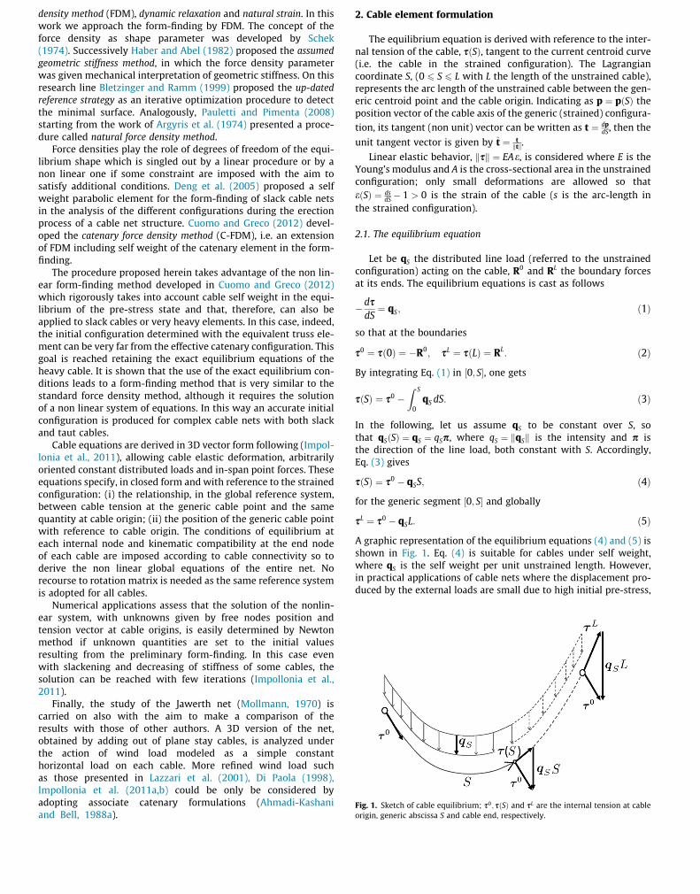
A graphic representation of the equilibrium equations (4) and (5) isshown in Fig. 1. Eq. (4) is suitable for cables under self weight,where qS is the self weight per unit unstrained length. However,in practical applications of cable nets where the displacement pro-duced by the external loads are small due to high initial pre-stress,

Fig. 1. Sketch of cable equilibrium; s0; sðSÞ and sL are the internal tension at cableorigin, generic abscissa S and cable end, respectively.

1522 L. Greco et al. / International Journal of Solids and Structures 51 (2014) 1521–1533


qS can also model wind loads. More general cases, such as those re-lated to the associate catenary cannot be correctly described by Eq.(4) and are discussed in Ahmadi-Kashani and Bell (1988a). In thefollowing the pedex S will be omitted and the load q is tacitely re-ferred to the unstrained configuration.

2.2. Elastic catenary solution

The equation governing the strained cable configuration isderived assuming uniform distributed load and also allowing thepresence of an additional in-span point force.

2.2.1. Uniform distributed loadThe equations of the equilibrated configuration of an extensible

cable are derived under the assumptions of perfect shear and bend-ing flexibility, following Impollonia et al. (2011). The case of a uni-form distributed load, q ¼ qp, is first considered.

The equilibrium equation for a segment ½0; S�, with S 6 L, isgiven by (4) where s0 ¼ fs0

x ; s0y ; s0

zg is the vector collecting thetension force components at cable origin. Recalling that thecable tension is a vector along the current tangent of the cableconfiguration, one has

t̂ðSÞ ¼ sðSÞksðSÞk ; ð6Þ

where, in virtue Eq. (4), the modulus of the tension is given by:

ksðSÞk ¼ ks0 � qSk: ð7Þ

It is not trivial to observe that this definition (as clear from Eq. (6))rules out compression for the cable. Furthermore, assuming linearelastic behavior and small deformation one gets

dsdS¼ ktk ¼ 1þ e ¼ 1þ ksðSÞk

EA: ð8Þ

Therefore, from Eqs. (6) and (8) the tangent vector splits in the sumof two addend

t ¼ dpdS¼ ktkt̂ ¼ 1þ ksðSÞk

EA

� �sðSÞksðSÞk ¼

sðSÞksðSÞk þ

sðSÞEA

: ð9Þ

The sought closed form of catenary equation,

pðSÞ ¼ pð0Þ þZ S

0tdS; ð10Þ

is obtained exploiting Eq. (9) and can be cast in the following form:

pðSÞ ¼ pð0Þ þ pCðSÞ þ pEðSÞ; ð11Þ

with

pCðSÞ ¼Z S

0

sðSÞksðSÞk dS; pEðSÞ ¼

1EA

Z S

0sðSÞdS; ð12Þ

where pð0Þ is cable origin position, pCðSÞ represents the unstrainedsolution while pEðSÞ gives the contribute of the elastic increment.The second integral can be easily solved, so to give:

pEðSÞ ¼qSEA

s0

q� p

S2

� �: ð13Þ

The first integral in Eq. (12) requires some manipulations that areexposed in Impollonia et al. (2011) and can be written as follows:

pCðSÞ ¼ ðI� ppTÞ s0

qln

qðSÞqð0Þ

� �� p

s0

q� pS

�� s0

q

��

� �; ð14Þ

where the function qðSÞ is defined as:

qðSÞ ¼ ksðSÞk � pTsðSÞ ¼ ks0 � qSk � pTðs0 � qSÞ: ð15Þ

Finally, the strained configuration of the cable is given by

pðSÞ ¼ qSEA

s0

q� p

S2

� �þ ðI� ppTÞ s

0

qln

qðSÞqð0Þ

� �

� ps0

q� pS

�� s0

q

��

� �þ pð0Þ: ð16Þ

Once s0 and pð0Þ are determined, the length of a strained segmentof the cable can be evaluated by means of Eq. (8):

sðSÞ ¼Z S

01þ sðSÞ

EA

� �dS ¼ Sþ DLðSÞ; ð17Þ

with the global elongation

DL ¼Z L

0

sðSÞEA

dS ð18Þ

and strained length of the cable l ¼ Lþ DL. Fig. 2 sketches thedefined quantities.

2.2.2. Additional one point forceLet us assume that one point force f is applied at abscissa �S on

the cable along with the distributed load q. The equilibrium equa-tion of the generic cable segment, analogous to (4), in this case isgiven by

sðSÞ ¼ s0 � fU½S� �S� � qS; ð19Þ

where U½S� �S� is the unit step function. For S 6 �S the equilibriumsolution reduces to that for cables with distributed load only, Eq.(16), while for S > �S, see Impollonia et al. (2011), the solution isgiven by

pðSÞ ¼ qEA

s0Sq� fðS� �SÞ

q� pS2

2

!þ ðI

� ppTÞ s0

qln

qð�SÞqFðSÞqð0ÞqFð�SÞ

" #� f

qln

qFðSÞqFð�SÞ

" # !

� ps0

q� f

q� pS

��þ s0

q� p�S

�� s0

q

�� s0

q� f

q� p�S

��

� �þ pð0Þ;

ð20Þ

with

qFðSÞ ¼ ks0 þ f � pSk � pTðs0 þ f � pSÞ: ð21Þ

An extended formula accounting for more point forces along thecable and thermal loads is available in Impollonia et al. (2011).

Fig. 2. Unstrained configuration (solid) with 0 6 S 6 L and strained configuration(dashed) with 0 6 s 6 l under uniformly distributed load.

L. Greco et al. / International Journal of Solids and Structures 51 (2014) 1521–1533 1523


3. Nodal equilibrium and compatibility conditions for cablestructures

The problem equations for cable nets are now defined. Theseare: (i) equilibrium equations at free nodes and (ii) compatibilityequations, which are expressed as connectivity conditions at theend node of each cable exploiting Eq. (16) or (20).

Assume that the cable net has N ¼ N1 þ N2 nodes, with N1 freenodes and N2 fixed nodes, and M cables. For the sake of simplicityfree nodes will be consecutively numbered from 1 to N1 whereasthe fixed nodes from N1 þ 1 to N. Let i be the generic free nodeof the net, with i ¼ 1;2; . . . N1, and j the generic cable connectedto the node j1 (origin of the cable) and j2 (end of the cable), withj ¼ 1;2; . . . M and j1; j2 ¼ 1;2 . . . N. The equilibrium of the ith node,joining ni cables, is given by

Xni

j

s�j

!þ Fi ¼ 0; ði ¼ 1;2; . . . N1Þ ð22Þ

where Fi is the external force applied to the node and s�j , if only dis-tributed load is present, is given by

s�j ¼þs0

j ; if j1¼ i; ði:e: the cable origin is at the nodeÞ

�sLj ¼� s0

j �qjLj

� �; if j2¼ i; ði:e: the cable end is at the nodeÞ

8><>:

ð23Þ

According to the connectivity of the net, the jth cable is joined tonodes j1 (cable origin) and j2 (cable end), so that the compatibilityequations relevant to the jth cable under uniform distributed loadare

pjð0Þ ¼ Xj1 ; pjðLjÞ ¼ Xj2 ; ð24Þ

being Xj1 and Xj2 the coordinates of the nodes of the net (free orfixed) in the strained configuration. The position of the cable endsis derived from Eq. (16) and is given by

pjðLjÞ ¼qjLj

EjAj

s0j

qj� pj

Lj

2

!þ I� pjp

Tj

� � s0j

qjln

qjðLjÞqjð0Þ

" #

� pj

s0j

qj� pjLj

�� s0

j

qj

��

!þ pjð0Þ; ðj ¼ 1;2 . . . MÞ: ð25Þ

Analogous equations can be written if a point force is acting on thecable referring to Eqs. (19) and (20). An example of equilibrium andcompatibility relationships is shown in Fig. 3.

Assume that unstrained length Lj, cross sectional area Aj, elas-tic modulus Ej and load qj be assigned for each cable and nodalforces Fi be given for each free node. Then, the 3N1 equilibriumequations (22) and the 3M compatibility conditions (25) realize anon linear set of equations with unknowns given by 3N1 coordi-nates of free nodes, Xi ¼ fXi;Yi; Zig, and 3M components of cabletension at cables origin, s0

j ¼ fs0j;x; s0

j;y; s0j;zg.

The system of equations allows the structural analysis ofthree dimensional cable nets under external nodal forces, uni-form distributed loads and point forces however oriented onthe cables. On the other hand it is not well suited for the initialdesign, i.e. the form-finding of the net, as the initial cablelengths must be imposed. The latter problem is tackled in thefollowing according to a strategy proposed in Cuomo and Greco(2012).

4. Form-finding

The form-finding strategy, named catenary force densitiesmethods, C-FDM, is resorted to. The strategy is based on the forcedensity method for slack cable nets and accounts for self weight inthe form-finding.

The procedure is clearly non-linear because the length of thecables are unknown so as their total weights. For this reason wefirst consider a linear step, i.e. the classical form-finding problemneglecting self weight, by linear force density method (L-FDM).The solution of the linear step is the initializing solution forthe successive non linear C-FDM. A uniform vertical conservativeloads acting on the cable, q ¼ qzpz, ia assumed for each cable(pz ¼ f0;0;�1g) as self-weight. The equilibrium equations ofthe ith node are

Xni

j

s�j;x ¼ 0;

Xni

j

s�j;y ¼ 0;

Xni

j

s�j;z ¼ 0:

ð26Þ

The following decomposition for the tensile force at cable origin isconsidered

s0j ¼ V0

j þH0j ; ð27Þ

where V0j and H0

j are vertical and horizontal vectors, respectively,given by

V0j ¼ pz p

Tz

s0

j ; H0j ¼ I� pz p

Tz

s0

j : ð28Þ

The horizontal components are

s0j;x ¼ sL

j;x ¼ H0j;x ¼ kH

0j k

Xj2 � Xj1

Dhj;

s0j;y ¼ sL

j;y ¼ H0j;y ¼ kH

0j k

Yj2 � Yj1

Dhj;

ð29Þ

where Dhj ¼ffiffiffiffiffiffiffiffiffiffiffiffiffiffiffiffiffiffiffiffiffiffiffiffiffiffiffiffiffiffiffiffiffiffiffiffiffiffiffiffiffiffiffiffiffiffiffiffiffiffiffiffiffiffiðXj2 � Xj1 Þ

2 þ ðYj2 � Yj1 Þ2

qis the horizontal span

between cable extremities. The vertical components of the tensilestress at the cable ends according to the catenary solution, seeCuomo and Greco (2012), are given by

Fig. 3. Equilibrium at node i and compatibility for cables connected to node i. Grayarrows are the forces acting on the node.



V0j ¼kH0

j kDhj

gj

Cosh½gj�Sinh½gj�

ðZj2 � Zj1 Þ �qz;jLj

2;

VLj ¼kH0

j kDhj

gj


ðZj2 � Zj1 Þ þqz;jLj

2;

ð30Þ

with

gj ¼qz;jDhj

2kH0j k: ð31Þ

By introducing the cable force density

Q j ¼kH0

j kDhj

; ð32Þ

the nodal equilibrium reduces to

Xni

j

� Q jðXj2 � Xj1 Þ ¼ 0;

Xni

j

� Q jðYj2 � Yj1 Þ ¼ 0;

Xni

j

qz;j

2�


ðZj2 � Zj1 Þ � Lj

!¼ 0;

ð33Þ

where the sign ðþÞmust be imposed if j1 ¼ i (i.e. the node is the ori-gin of the jth cable), whereas the sign ð�Þ should be retained if j2 ¼ i(i.e. the node is the end of the jth cable).

The unstrained length of the jth cable is given by

Lj ¼ lj � DLe;j; ð34Þ

where the length of the strained cable is

lj ¼

ffiffiffiffiffiffiffiffiffiffiffiffiffiffiffiffiffiffiffiffiffiffiffiffiffiffiffiffiffiffiffiffiffiffiffiffiffiffiffiffiffiffiffiffiffiffiffiffiffiffiffil2j

g2j

Sinh½gj� þ ðZj2 � Zj1 Þ2

vuut ð35Þ

and the elastic increment (DLe;j) is given by

DLe;jðkH0j k;V

0j ; LjÞ ¼

lðV0j Þ � lðVL

j Þ2EAqz;j

: ð36Þ

The operator lð�Þ is given by

lð�Þ ¼ ð�Þffiffiffiffiffiffiffiffiffiffiffiffiffiffiffiffiffiffiffiffiffiffiffiffiffiffiffið�Þ2 þ kH0

j k2

qþ kH0

j k2ArcSinh

ð�ÞkH0

j k

!: ð37Þ

By substituting Eq. (34) into (33) a non linear set of equations withunknown fXi;Yi; Zig is obtained when the force density is assignedat each cable.

The solution of the form-finding neglecting self weight, accord-ing to L-FDM, i.e. the solution of the following linear system

Xni

j

� Q jðXj2 � Xj1 Þ ¼ 0;

Xni

j

� Q jðYj2 � Yj1 Þ ¼ 0;

Xni

j

� Q jðZj2 � Zj1 Þ ¼ 0;

ð38Þ

is adopted as the initial step for the solution of the non linear equi-librium equations (33).

5. Numerical examples

The capabilities of the proposed procedure are preliminarilyassessed by examining a simple slack cable net, first designed bythe proposed C-FDM and successively loaded with a nodal forceand a point force along a cable. Finally, the procedure is appliedto the form-finding and successive structural analysis of a net inpresence of struts. Namely, the plane Jawerth cable structure(Mollmann, 1970) is analyzed along with its spatial version, wherethe effectiveness of the proposed strategy is fully exploited.

5.1. A 5-cable net

The simple very slack 5-cable net reported in Fig. 4(a) is consid-ered. A form-finding by means of C-FDM is first performed, thenstarting from the obtained configuration two load cases areapplied: a nodal force and one point force on a cable.

Fig. 4. Initial configuration, topology and labels of nodes and cables of the cable net (a); different configurations at the load Fy ¼ 0;�3;�10 [daN], respectively plotted withcontinuous, dashed and pointed line (b).



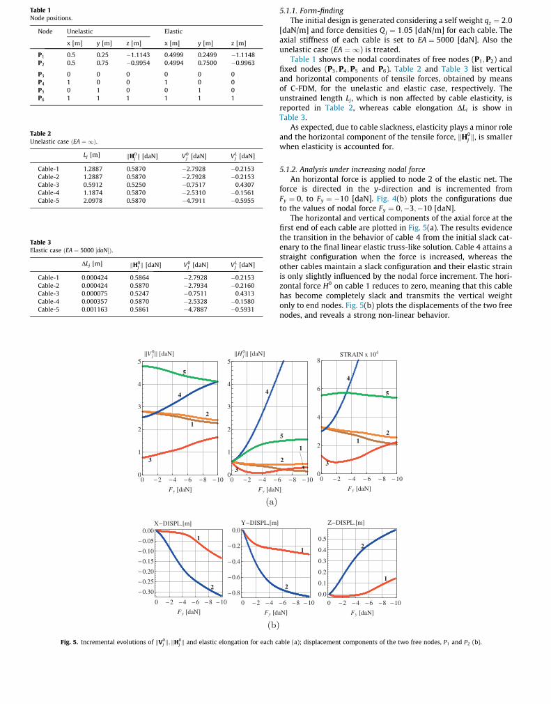
5.1.1. Form-findingThe initial design is generated considering a self weight qz ¼ 2:0

[daN/m] and force densities Q j ¼ 1:05 [daN/m] for each cable. Theaxial stiffness of each cable is set to EA ¼ 5000 [daN]. Also theunelastic case (EA ¼ 1) is treated.

Table 1 shows the nodal coordinates of free nodes (P1;P2) andfixed nodes (P3;P4;P5 and P6). Table 2 and Table 3 list verticaland horizontal components of tensile forces, obtained by meansof C-FDM, for the unelastic and elastic case, respectively. Theunstrained length Lj, which is non affected by cable elasticity, isreported in Table 2, whereas cable elongation DLi is show inTable 3.

As expected, due to cable slackness, elasticity plays a minor roleand the horizontal component of the tensile force, kH0

j k, is smallerwhen elasticity is accounted for.

5.1.2. Analysis under increasing nodal forceAn horizontal force is applied to node 2 of the elastic net. The

force is directed in the y-direction and is incremented fromFy ¼ 0, to Fy ¼ �10 [daN]. Fig. 4(b) plots the configurations dueto the values of nodal force Fy ¼ 0;�3;�10 [daN].

The horizontal and vertical components of the axial force at thefirst end of each cable are plotted in Fig. 5(a). The results evidencethe transition in the behavior of cable 4 from the initial slack cat-enary to the final linear elastic truss-like solution. Cable 4 attains astraight configuration when the force is increased, whereas theother cables maintain a slack configuration and their elastic strainis only slightly influenced by the nodal force increment. The hori-zontal force H0 on cable 1 reduces to zero, meaning that this cablehas become completely slack and transmits the vertical weightonly to end nodes. Fig. 5(b) plots the displacements of the two freenodes, and reveals a strong non-linear behavior.

Table 2Unelastic case ðEA ¼ 1Þ.

Lj [m] kH0j k [daN] V0

j [daN] VLj [daN]

Cable-1 1.2887 0.5870 �2.7928 �0.2153Cable-2 1.2887 0.5870 �2.7928 �0.2153Cable-3 0.5912 0.5250 �0.7517 0.4307Cable-4 1.1874 0.5870 �2.5310 �0.1561Cable-5 2.0978 0.5870 �4.7911 �0.5955

Table 3Elastic case ðEA ¼ 5000 ½daN�Þ.

DLj [m] kH0j k [daN] V0

j [daN] VLj [daN]

Cable-1 0.000424 0.5864 �2.7928 �0.2153Cable-2 0.000424 0.5870 �2.7934 �0.2160Cable-3 0.000075 0.5247 �0.7511 0.4313Cable-4 0.000357 0.5870 �2.5328 �0.1580Cable-5 0.001163 0.5861 �4.7887 �0.5931

0 2 4 6 8 100

1

2

3

4

5

Fy daN

V j0 daN

0 2 4 6 8 100

1

2

3

4

5

Fy daN

H j0 daN

0 2 4 6 8 100

2

4

6

8

Fy daN

STRAIN x 104

5

5

54 4

4

2

2

21

11

3

33

(a)

0 2 4 6 8 10

0.30

0.25

0.20

0.15

0.10

0.05

0.00

Fy daN

X DISPL. m

0 2 4 6 8 10

0.8

0.6

0.4

0.2

0.0

Fy daN

Y DISPL. m

0 2 4 6 8 100.0

0.1

0.2

0.3

0.4

0.5

Fy daN

Z DISPL. m

1

1

12 2

2

(b)

Fig. 5. Incremental evolutions of kV0j k; kH

0j k and elastic elongation for each cable (a); displacement components of the two free nodes, P1 and P2 (b).

Table 1Node positions.

Node Unelastic Elastic

x [m] y [m] z [m] x [m] y [m] z [m]

P1 0.5 0.25 �1.1143 0.4999 0.2499 �1.1148P2 0.5 0.75 �0.9954 0.4994 0.7500 �0.9963

P3 0 0 0 0 0 0P4 1 0 0 1 0 0P5 0 1 0 0 1 0P6 1 1 1 1 1 1



In particular the stiffening effects due to cable 4 is evident fromthe y-displacement plot.

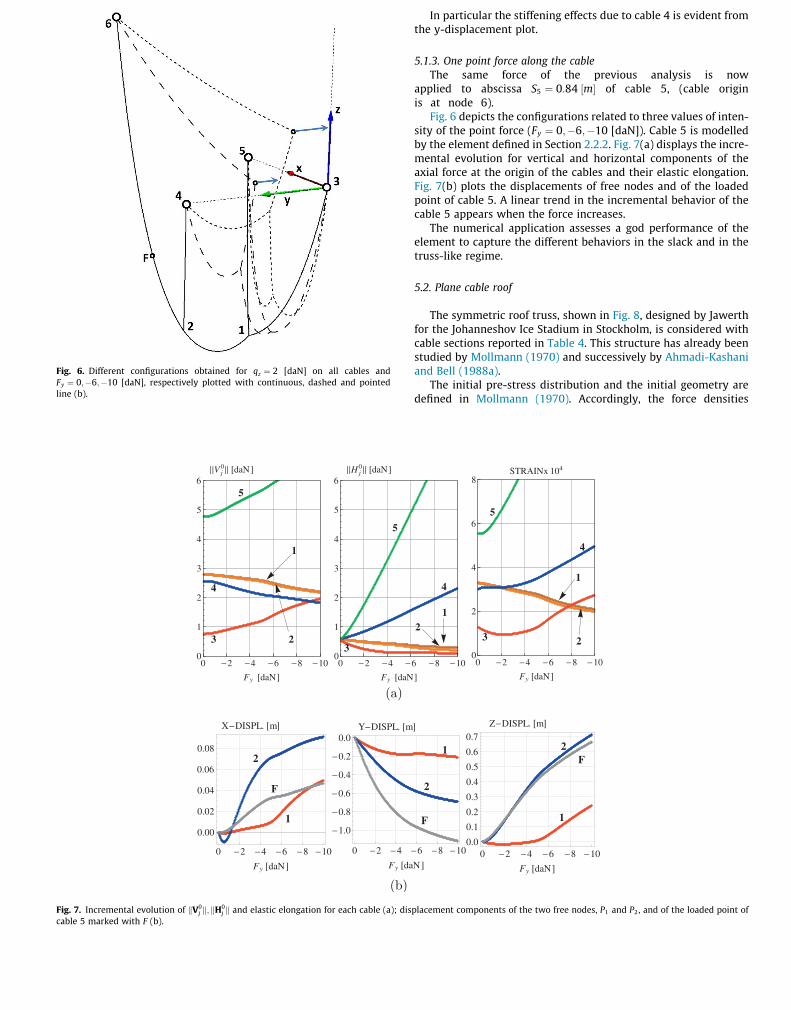
5.1.3. One point force along the cableThe same force of the previous analysis is now

applied to abscissa S5 ¼ 0:84 ½m� of cable 5, (cable originis at node 6).

Fig. 6 depicts the configurations related to three values of inten-sity of the point force (Fy ¼ 0;�6;�10 [daN]). Cable 5 is modelledby the element defined in Section 2.2.2. Fig. 7(a) displays the incre-mental evolution for vertical and horizontal components of theaxial force at the origin of the cables and their elastic elongation.Fig. 7(b) plots the displacements of free nodes and of the loadedpoint of cable 5. A linear trend in the incremental behavior of thecable 5 appears when the force increases.

The numerical application assesses a god performance of theelement to capture the different behaviors in the slack and in thetruss-like regime.

5.2. Plane cable roof

The symmetric roof truss, shown in Fig. 8, designed by Jawerthfor the Johanneshov Ice Stadium in Stockholm, is considered withcable sections reported in Table 4. This structure has already beenstudied by Mollmann (1970) and successively by Ahmadi-Kashaniand Bell (1988a).

The initial pre-stress distribution and the initial geometry aredefined in Mollmann (1970). Accordingly, the force densities

0 2 4 6 8 100

1

2

3

4

5

6

Fy daN

V j0 daN

0 2 4 6 8 100

1

2

3

4

5

6

Fy daN

H j0 daN

0 2 4 6 8 100

2

4

6

8

Fy daN

STRAINx 104

5

5

5

1

1

1

22

2

4 4

4

33

3

(a)

0 2 4 6 8 10

0.00

0.02

0.04

0.06

0.08

Fy daN

X DISPL. m

0 2 4 6 8 10

1.0

0.8

0.6

0.4

0.2

0.0

Fy daN

Y DISPL. m

0 2 4 6 8 100.0

0.1

0.2

0.3

0.4

0.5

0.6

0.7

Fy daN

Z DISPL. m

2

2

2

1

1

1

F

F

F

(b)

Fig. 7. Incremental evolution of kV0j k; kH

0j k and elastic elongation for each cable (a); displacement components of the two free nodes, P1 and P2, and of the loaded point of

cable 5 marked with F (b).

Fig. 6. Different configurations obtained for qz ¼ 2 [daN] on all cables andFy ¼ 0;�6;�10 [daN], respectively plotted with continuous, dashed and pointedline (b).



Qj ¼ kH0j k=Dhj have been evaluated for top, bottom and diagonal

cables and reported in Table 5. The modulus of elasticityE ¼ 14790 [kN/cm2] is assumed for all the elements (includingcolumns). As in Ahmadi-Kashani and Bell (1988a), element selfweight is determined assuming a density q ¼ 77:784 [kN/m3].

The unstrained lengths of stays (element n. 1, 2, 37, 40) andcolumns (element n. 3, 5, 36, 39) are determined imposing thecoordinates of their end nodes (see Fig. 8), and equilibrium atnodes 3, 4 and 21, 22. The unstrained length for the elements islisted in Table 6.

First we compare our results with those obtained by Mollmann(1970) and successively by Ahmadi-Kashani and Bell (1988a),referred to a dead load of the roof equal to 1:786 [kN/m] andapplied to top cable. The unstrained lengths are those given inTable 6. Table 7 shows the results obtained by Mollmann (1970)and Ahmadi-Kashani and Bell (1988a) and the proposed strategy

for the considered load case. As appears from Table 7 there areno significative differences in the results obtained for top, bottomand stay cables (i.e. taut elements).

Table 4Cross sections.

Element group Area [cm2]

Top cable 25.1Bottom cable 17.2Diagonals 2.84Longer stays 63.7Shorter stays 15.9Columns 222.6

Table 5Force density Q j .

Top [kN/m] Bottom [kN/m] Diagonal [kN/m]

Q6 ¼ 68:397 Q9 ¼ 42:217 Q4 ¼ 2:110Q8 ¼ 51:695 Q13 ¼ 70:291 Q7 ¼ 2:261Q12 ¼ 77:494 Q17 ¼ 82:825 Q10 ¼ 5:422Q16 ¼ 122:404 Q20 ¼ 35:065 Q11 ¼ 2:507Q19 ¼ 55:249 Q14 ¼ 8:436

Q15 ¼ 1:748Q18 ¼ 30:431

Table 6Unstrained length Lj .

Top [m] Bottom [m] Diagonal [m] Columns [m] Stays [m]

L6 ¼ 7:692 L9 ¼ 13:142 L4 ¼ 10:510 L3 ¼ 3:799 L1 ¼ 14:807L8 ¼ 10:124 L13 ¼ 7:742 L7 ¼ 7:558 L5 ¼ 9:098 L2 ¼ 8:201L12 ¼ 6:863 L17 ¼ 6:265 L10 ¼ 5:743L16 ¼ 4:555 L20 ¼ 13:169 L11 ¼ 4:068L19 ¼ 11:163 L14 ¼ 4:090

L15 ¼ 2:815L18 ¼ 2:168

Table 7Element forces under dead load.

el. group n. Mollmann(1970) [tons]

Ahmadi-Kashani andBell (1988a) [tons]

Presentanalysis[tons]

Columns 3 �151:9 �154:63 �153:475 �137:9 �139:40 �138:03

Stays 1 140:5 140:00 141:062 46:4 46:97 47:34

Top-c. 6 70:9 70:71 71:168 69:6 69:22 68:3712 69:1 68:70 69:5416 68:9 68:48 69:3619 72:3 72:15 73:15

Bottom-c.

9 41:5 41:55 41:7513 41:4 41:50 41:3617 41:1 41:19 40:9520 38:6 38:54 37:89

Diagonals 4 1:00 1:00 1:407 1:80 2:00 1:3810 1:40 1:50 0:9711 1:40 1:51 1:1014 1:40 1:50 1:1115 1:40 1:47 2:6518 3:90 4:18 5:21

Fig. 8. Geometry of the Jawerth cable truss with node labels (a) and cable labels (b).



Let us now consider the load case defined by vertical forces ap-plied to the nodes of half top cable with intensity F. In order toshow the performance of the numerical procedure, the intensityof the force is increased from F ¼ 0 to F ¼ 57:8 [kN]. The initialand final configurations of the cable-net are shown in Fig. 9. Theunloading of diagonals, especially those under vertical nodalforces, is evident.

The ratio ks0k=ks0pre�stressk, where s0 is the tensile force in

the loaded configuration and s0pre�stress is the same quantity

for F ¼ 0, are reported in Figs. 10 and 11. As expected, thetensile force of the top cable increases with the load; anhigher increment is shown for the loaded side of the net (leftside), see Fig. 10(a). On the other hand, the bottom cableshows a reduction of the tensile force when the load increases,see Fig. 10(b).

A more complex scenario appears for the diagonals. Some ofthem become slack (elements n. 4, 10, 14, 18, 23 and 27) whenthe force increases, see Fig. 11(a). Diagonals n. 11 and 15 exhibit

68121619

2225293338

57.8 28.9 0 28.9 57.80.8

1.0

1.2

1.4

1.6

1.8

2.0

2.2

F kN

left side of the net T O P C A B L E right side of the net

(a)

9131732

21242832

57.8 28.9 0 28.9 57.80.2

0.4

0.6

0.8

1.0

F kN

left side of the net B O T T O M C A B L E right side of the net

(b)

Fig. 10. Results of the incremental analysis for top cables (a) and bottom cables (b).

Fig. 9. Initial (F ¼ 0) and final (F ¼ 57:8 ½kN�) configurations of the net.



a non monotonous trend for increasing forces; high sensitivity ofthe tensile force at diagonal n. 26 is evident. It can be observed thatdiagonal cables are most affected by node force increments whencompared with other cables.

Finally, Fig. 11(b) shows that shorter stay cables (element n. 2and 37) lose tension when nodal forces increases, whereasan opposite trend is shown by longer stay cables. The axial

compressive force increment on columns is basically linearlyrelated to nodal force intensity.

5.3. Space cable roof

The structure of the previous section is investigated for a differ-ent configuration of the stay cables. These are now positioned outof the main vertical plane (the plane containing all free nodes), asshown in Fig. 12, where half of the symmetric three-dimensionalcable roof is depicted. The net is now capable to withstand hori-zontal actions along y-direction. The longer stays have unstrainedlength L1 ¼ L21 ¼ 16:50 [m]; for the shorter ones L2 ¼ L22 ¼10:96 [m]. The other elements of the structure are defined as inthe previous section, since the same force densities are adopted(see Table 5 and first four columns of Table 6).

A structural analysis is conducted under an incremental hori-zontal load (orthogonal to the main vertical plane) uniform oneach element of the net (cables and columns) and defined asqj ¼ k � qref � /j, where /j is the diameter of the element,qref ¼ 2:6 [kN/m] and the load factor k 2 ½0;1�. The load conditioncould be a rough model of wind action on the net. The columns

Fig. 11. Results of the incremental analysis for diagonal cables (a) and stay cables and columns (b).

Fig. 12. Labels of half 3D cable roof.



have hollow circular cross section with diameter / ¼ 0:5 [m],whereas all the cables have solid circular section and their diame-ter can deduced by Table 4.

The results of the incremental analysis are reported in Figs. 13–16 and the final configuration (k ¼ 1) is depicted in Fig. 13(a).

The onset of the out-plane load is balanced by up-wind staysas only the tension of cables 21 and 22 exhibit a promptincrement, whereas down-wind stays are initially unloaded (see

Fig. 14(b)). All the other elements do not vary appreciably theirtension when the load factor is small. In fact as depicted inFigs. 13(b), 14(a), 15(a) and 15(b) an horizontal tangent appearsfor k! 0. When k increases the stiffness gain is evident and ten-sile stress rises in all elements but in the longer down-wind stay(element n.1). The geometric stiffening behavior is evident fromthe trend of y-displacement of the center of the net plotted inFig. 16.

40

20

0

20

40

5 0 5

10

5

0

(a)

5

3

0 0.25 0.5 0.75 1

1.9

1.8

1.7

1.6

1.5

1.4

1.3

1.2

load factor λ

Axi

alFo

rce

MN

COLUMNS

(b)

Fig. 13. Results of the incremental analysis: final configuration of the net (a) and compressive axial force on the columns (b).

19

16

12

8

6

0 0.25 0.5 0.75 1

0.7

0.8

0.9

1.

load factorλ

τ0MN

TOP CABLES

(a)

21

22

12

0 0.25 0.5 0.75 1

0.6

0.7

0.8

0.9

1.

1.1

load factorλ

τ0MN

STAY CABLES

(b)

Fig. 14. Results of the incremental analysis: tensile force at the first end for top (a) and stay cables (b).



6. Conclusions

A general procedure has been developed which can accuratelysolve cable structures under different load conditions. The proce-dure relies on the three dimensional vector form solution of thecatenary equation which allows a straight derivation of compati-bility conditions in the global reference system. Both the case ofuniformly distributed load and point force generally oriented inspace can be handled. The non-linear algebraic governing equa-tions with unknowns given by cable tension components andfree node coordinates are easily assembled according to cableconnectivity and position of fixed nodes. The numerical solutionmay be conveniently pursued by the Newton–Raphson methodby choosing suitable initial conditions under cable pre-stress andself weight. To this aim the catenary force density method isresorted to in order to determine the initial cable stresses and

configuration of the net. The effectiveness of the method is shownfor slack cable nets, the plane Jawerth cable net and its threedimensional version.

References

Ahmadi-Kashani, K., Bell, A.J., 1986. The representation of cables subjected togeneral loading. Int. J. Space Struct. 2, 29–44.

Ahmadi-Kashani, K., Bell, A.J., 1988a. The analysis of cables subject to uniformlydistributed loads. Eng. Struct. 10 (3), 174–184.

Ahmadi-Kashani, K., Bell, A.J., 1988b. Representation of cables in space subjected touniformly distributed loads. Int. J. Space Struct. 3 (4), 221–230.

Andreu, A., Gil, L., Roca, P., 2006. A new deformable catenary element for theanalysis of cable net structures. Comput. Struct. 84 (29–30), 1882–1890.

Argyris, J.H., Angelopoulos, T., Bichat, B., 1974. A general method for shape findingof lightweight tension structures. Comput. Methods Appl. Mech. Eng. 30, 263–284.

Bletzinger, K.U., Ramm, E., 1999. A general finite element approach to the formfinding of tensile structures by the updated reference strategy. Int. J. SpaceStruct. 14 (2), 131–146.

Bruno, D., Leonardi, A., 1999. A nonlinear structural models in cableway transportsystem. Simul. Pract. Theor. 7 (3), 207–218.

Cuomo, M., Greco, L., 2012. On the force density method for slack cable nets. Int. J.solids Struct. 49 (13), 1526–1540.

Deng, H., Jiang, Q., Kwan, A., 2005. Shape finding of incomplete cable-strutassemblies containing slack and prestressed elements. Comput. Struct. 83,1767–1779.

Di Paola, M., 1998. Non-linear dynamic analysis of cable-suspended structuressubjected to wind actions. J. Wind Eng. Ind. Aerodyn. 74–79, 91–109.

Freire, A.M.S., Negrão, J.H.O., Lopes, A.V., 2006. Geometrical nonlinearities on thestatic analysis of highly flexible cable-stayed bridges. Comput. Struct. 84, 2128–2140.

Haber, R., Abel, J., 1982. Initial equilibrium solution methods for cable reinforcedmembranes part ii-implementation. Comput. Methods Appl. Mech. Eng. 30,285–306.

Impollonia, N., Ricciardi, G., Saitta, F., 2011. Static of elastic cables under 3d pointforces. Int. J. Solid Struct. 48, 1268–1276.

Impollonia, N., Ricciardi, G., Saitta, F., 2011a. Vibrations of inclined cables underskew wind. Int. J. Non-Linear Mech. 46 (7), 907–919.

Impollonia, N., Ricciardi, G., Saitta, F., 2011b. Dynamics of shallow cables underturbulent wind: a nonlinear finite element approach. Int. J. Struct. Stab. Dyn. 11(4), 755–774.

Irvine, H.M., 1992. Cable Structures. Dover Publications, New York.Jayaraman, H.B., Knudson, W.C., 1981. A curved element for the analysis of cable

structures. Comput. Struct. 14 (3–4), 325–333.Lazzari, M., Saetta, A., Vitaliani, R., 2001. Non-linear dynamic analysis of cable-

suspended structures subjected to wind actions. Comput. Struct. 79 (9), 953–969.

18

14104

15119

0 0.25 0.5 0.75 1

0.02

0.04

0.06

0.08

0.1

load factor λ

τ0MN

DIAGONAL CABLES

(a)

9

13

17

20

0 0.25 0.5 0.75 1

0.6

0.7

0.8

0.9

load factor λ

τ0MN

BOTTOM CABLES

(b)

Fig. 15. Results of the incremental analysis: tensile force at the first end of the diagonal (a) and bottom cables (b).

10 uz

uy

0.0 0.2 0.4 0.6 0.8 1.0 1.2 1.40

0.2

0.4

0.6

0.8

1

displacements m

load

fact

orλ

Fig. 16. Displacement at the center of the net versus load factor.



Lee, C.L., Perkins, N.C., 1992. Oscillations of suspended cables containing a two-to-one internal resonance. Nonlinear Dyn. 3, 465–490.

Lepidi, M., Gattulli, V., Vestroni, F., 2007. Static and dynamic response of elasticsuspended cables with damage. Int. J. Solid Struct. 44 (25–26), 8194–8212.

Luongo, A., Piccardo, G., 1998. Non-linear galloping of sagged cables in 1:2 internalresonance. J. Sound Vib. 214 (5), 915–936.

Luongo, A., Piccardo, G., 2008. A continuous approach to the aeroelastic stability ofsuspended cables in 1:2 internal resonance. J. Vib. Control 14 (1–2), 135–157.

Mollmann, H., 1970. Analysis of plane prestressed cable structures. J. Struct. Div.ASCE 96 (ST10), 2059–2082.

Pauletti, R., Pimenta, P., 2008. The natural force density method for theshape finding of taut structures. Comput. Methods Appl. Mech. Eng. 197,4419–4428.

Peyrot, A.H., Goulois, A.M., 1978. Analysis of flexible transmission lines. J. Struct.Div. ASCE 104 (ST5), 763–779.

Peyrot, A.H., Goulois, A.M., 1979. Analysis of cable structures. Comput. Struct. 10 (5),805–813.

Sagatun, S., 2001. The elastic cable under the action of concentrated and distributedforces. J. Offshore Mech. Arct. Eng. 123 (1), 43–45.

Schek, H.J., 1974. The force density method for form finding and computation ofgeneral networks. Comput. Methods Appl. Mech. Eng. 3, 115–134.

Such, M., Jimenez-Octavio, J., Carnicero, A., Lopez-Garcia, O., 2009. An approachbased on the catenary equation to deal with static analysis of three dimensionalcable structures. Eng. Struct. 31 (9), 2162–2170.

Thai, H.T., Kim, S.E., 2011. Nonlinear static and dynamic analysis of cable structures.Finite Elem. Anal. Des. 47 (3), 237–246.


a procedure for the static analysis of cable structures ... · pdf filea procedure for the...

Documents