a probabilistic analysis of misparking in reservation ...inets/papers/ashok-msthesis-2011.pdf ·...
TRANSCRIPT
A PROBABILISTIC ANALYSIS OF MISPARKING IN
RESERVATION BASED PARKING GARAGES
by
Vikas G AshokB.E. Aug 2009, Visveswaraiah Technological University
A Thesis Submitted to the Faculty ofOld Dominion University in Partial Fulfillment of the
Requirement for the Degree of
MASTER OF SCIENCE
COMPUTER SCIENCE
OLD DOMINION UNIVERSITYApril 2011
Approved by:
Stephan Olariu (Director)
Michele Weigle
Tameer Nadeem
ABSTRACT
A PROBABILISTIC ANALYSIS OF MISPARKING IN
RESERVATION BASED PARKING GARAGES
Vikas G Ashok
Old Dominion University, 2011
Director: Dr. Stephan Olariu
Parking in major cities is an expensive and annoying affair, the reason ascribed to
the limited availability of parking space. Modern parking garages provide parking
reservation facility, thereby ensuring availability to prospective customers. Mispark-
ing in such reservation based parking garages creates confusion and aggravates driver
frustration. The general conception about misparking is that it tends to completely
cripple the normal functioning of the system leading to chaos and confusion. A single
mispark tends to have a ripple effect and therefore spawns a chain of misparks. The
chain terminates when the last mispark occurs at the parking slot reserved by the
first member of the misparking chain. Of interest is the probability distribution of
the random variable that represents the length of the misparking chain. The most
probable length of the chain as determined from the underlying probability distribu-
tion is therefore indicative of the extent of instability caused by a single mispark. In
this thesis, reasonably tight bounds for the probability of occurance of a misparking
chain of a given length are first determined. Next, the probability distribution of the
length of misparking chain is approximated. It can be inferred from the mathematical
derivations presented in this work that the most probable misparking chain length is
very small compared to the size of the garage, thereby showing that a mispark has
negligible effect on the stability of the parking system. Simulation results are also
presented to validate the analytical solutions.

c©Copyright, 2011, by Vikas G Ashok, All Rights Reserved
iii

ACKNOWLEDGEMENTS
My thesis work would not have been as satisfying and rewarding without the help of
my professors and friends in this university. I would like to thank everyone who has
been a part of this journey of mine. I am grateful to Dr. Stephan Olariu for all the
support, assistance, motivation and guidance which helped me successfully complete
this thesis. I thank Dr. Olariu for sharing some of the interesting research ideas
and problems that motivated me to pursue a research oriented career. He helped me
understand some of the advanced concepts in probability theory and linear algebra,
without which i could not have completed this work.
I extend my gratitude to my committee members, Dr. Michelle Weigle and Dr.
Tameer Nadeem for their valuable inputs and suggestions. I thank Mr. Ajay Gupta
for offering me a research assistantship position and an opportunity to work in the
Networks Research Laboratory. Most importantly, thanks to the Computer Science
Department at Old Dominion University for all the resources and help. My family
has always been supportive of my work and I would like to take this opportunity to
appreciate their love and concern.
I learnt a great lot working on this thesis and I’ll cherish this experience through-
out my life.
iv
v
TABLE OF CONTENTS
PageLIST OF FIGURES . . . . . . . . . . . . . . . . . . . . . . . . . . . . . . . . vi
CHAPTERS
I Introduction . . . . . . . . . . . . . . . . . . . . . . . . . . . . . . . . . . 1II State of the Art . . . . . . . . . . . . . . . . . . . . . . . . . . . . . . . . 3III Probabilistic Analysis of Misparking . . . . . . . . . . . . . . . . . . . . 4
III.1 System Model and Problem Statement . . . . . . . . . . . . . . . . . 4III.1.1 System Model . . . . . . . . . . . . . . . . . . . . . . . . . . . 4III.1.2 Problem Statement . . . . . . . . . . . . . . . . . . . . . . . . 4
III.2 Some Important Results . . . . . . . . . . . . . . . . . . . . . . . . . 4III.3 Upper Bound (UB) on Pr{L = l} . . . . . . . . . . . . . . . . . . . . 9III.4 Lower Bound (LB) on Pr{L = l} . . . . . . . . . . . . . . . . . . . . 12III.5 Most Probable Misparking Chain Length . . . . . . . . . . . . . . . . 13III.6 Simulation Results . . . . . . . . . . . . . . . . . . . . . . . . . . . . 14
IV A Recursive Solution . . . . . . . . . . . . . . . . . . . . . . . . . . . . . 21IV.1 First driver initiating mispark . . . . . . . . . . . . . . . . . . . . . . 21
IV.1.1 An Approximate Solution . . . . . . . . . . . . . . . . . . . . 22IV.1.2 Most Probable Chain Length Estimate . . . . . . . . . . . . . 25IV.1.3 Results . . . . . . . . . . . . . . . . . . . . . . . . . . . . . . . 25
V Summation of terms involving harmonic series . . . . . . . . . . . . . . . 29
V.1 Computation of∑n
k=1Hk
kand
∑nk=1
H2k
k. . . . . . . . . . . . . . . . . 29
V.2 Comptutation of∑n
k=1
Hpk
k,p > 0 . . . . . . . . . . . . . . . . . . . . . 34
V.2.1 Evaluating Coefficients . . . . . . . . . . . . . . . . . . . . . . 37
V.3 Properties of∑n
k=1
Hpk
k. . . . . . . . . . . . . . . . . . . . . . . . . . 40
VI Conclusion . . . . . . . . . . . . . . . . . . . . . . . . . . . . . . . . . . . 46
BIBLIOGRAPHY . . . . . . . . . . . . . . . . . . . . . . . . . . . . . . . . . 47
APPENDICES
A Review of some important formulae . . . . . . . . . . . . . . . . . . . . . 49A.1 ex . . . . . . . . . . . . . . . . . . . . . . . . . . . . . . . . . . . . . . 49A.2 an − bn . . . . . . . . . . . . . . . . . . . . . . . . . . . . . . . . . . . 49A.3 Limits . . . . . . . . . . . . . . . . . . . . . . . . . . . . . . . . . . . 49A.4 Poisson Random Variable . . . . . . . . . . . . . . . . . . . . . . . . 49
VITA . . . . . . . . . . . . . . . . . . . . . . . . . . . . . . . . . . . . . . . . 50
vi
LIST OF FIGURES
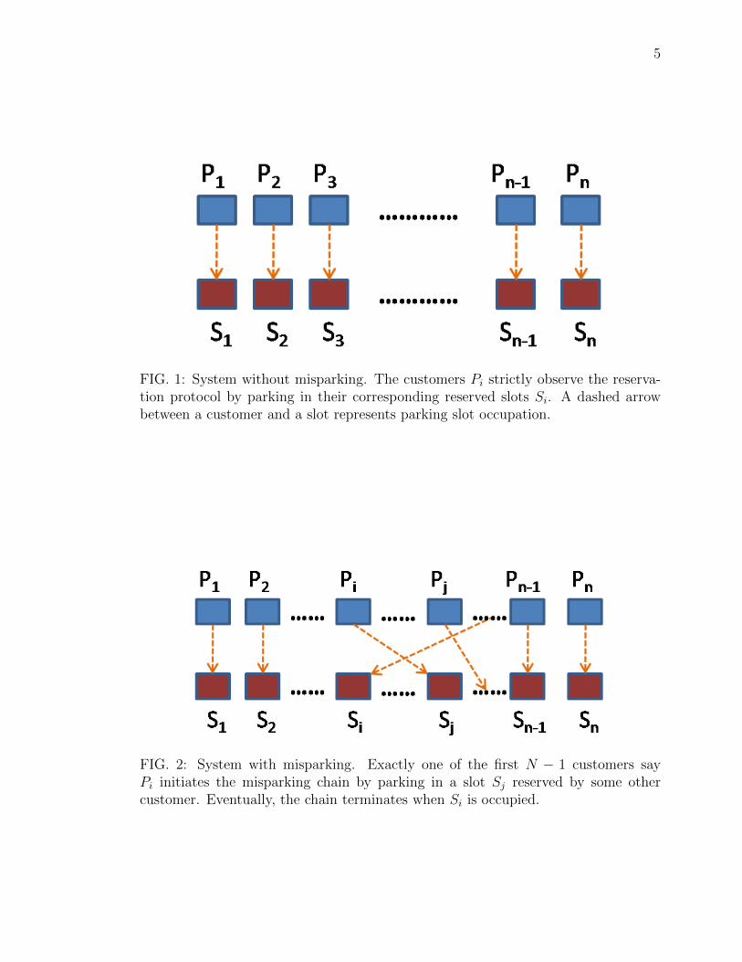
Page1 System without misparking. The customers Pi strictly observe the
reservation protocol by parking in their corresponding reserved slotsSi. A dashed arrow between a customer and a slot represents parkingslot occupation. . . . . . . . . . . . . . . . . . . . . . . . . . . . . . . 5
2 System with misparking. Exactly one of the first N − 1 customerssay Pi initiates the misparking chain by parking in a slot Sj reservedby some other customer. Eventually, the chain terminates when Si isoccupied. . . . . . . . . . . . . . . . . . . . . . . . . . . . . . . . . . . 5
3 Bounds vs simulation results, n = 500,s = 100000. . . . . . . . . . . . 154 Bounds vs simulation results, n = 500,s = 1000000. . . . . . . . . . . 165 Tightness of Bounds for n = 500, s = 100000 and s = 1000000. . . . . 166 Bounds vs simulation results, n = 1000,s = 100000. . . . . . . . . . . 177 Bounds vs simulation results, n = 1000,s = 1000000. . . . . . . . . . . 178 Tightness of Bounds for n = 1000, s = 100000 and s = 1000000. . . . 189 Bounds vs simulation results, n = 5000,s = 50000. . . . . . . . . . . . 1810 Bounds vs simulation results, n = 1000,s = 100000. . . . . . . . . . . 1911 Tightness of Bounds for n = 5000, s = 50000 and s = 100000. . . . . 1912 Simulation vs Approximation, n = 1000. . . . . . . . . . . . . . . . . 2513 Simulation vs Approximation, n = 3000. . . . . . . . . . . . . . . . . 2614 Simulation vs Approximation, n = 5000. . . . . . . . . . . . . . . . . 2615 Simulation vs Approximation, n = 7000. . . . . . . . . . . . . . . . . 2716 Difference between simulation and approximation. . . . . . . . . . . . 2717 Average difference between simulation and approximation. . . . . . . 28
1
CHAPTER I
INTRODUCTION
Parking assistance, currently is a hot topic of research. This can be attributed
to the increasing demand for parking in major cities where parking is limited and
costly. High contention for parking space spawns a need to deploy intelligent parking
systems in order to provide parking assistance to customers. Without any parking
assistance, locating a vacant parking slot in a heavily occupied parking garage is
a time consuming and frustrating affair. As the contention for parking space is
extremely high in major cities, a general and simple solution would be to provide
reservation facility to customers. Reservation gaurantees parking space and avoids
traffic congestion in parking garages. In addition, the driver is clearly aware of the
slot assigned to him/her, which eliminates the trouble of locating an empty slot
and therefore saves time. A wide variety of present day solutions rely on parking
reservation as the basis.
One of the common characteristics of the present day parking systems is that they
all assume ideal human behavior. In other words, customers are assumed to strictly
adhere to the rules laid out by the parking assistance mechanism. This assumption
is true in general but there can be exceptions. Misparking is one such exception that
tends to destabilize any reservation based parking system. A customer may choose to
park in a slot different from that reserved by him for his own convenience. However,
it is to be noted that misparking is a rare event as there are often severe penal-
ties(fine, towing, etc) associated with it. Nonetheless, it is still important to assess
the damage or instability caused by misparking. Intuition tells us that misparking
leads to chaos and confusion. Therefore, it of interest to determine both theoretically
and experimentally if our intuition is correct. This requires a mathematical model
to be defined to represent misparking.
In this work, the impact of misparking is analyzed in terms of length of the chain
produced by a single initial mispark as this chain length is indicative of the extent of
instability caused. Suppose, a driver A decides to park in a slot different from the slot
reserved by him for his own convenience or purpose. This in turn triggers another
mispark as one of the subsequent drivers B will find his assigned slot occupied and
therefore is forced to park in a different slot. At this point, two possibilities exist.
Either driver B can terminate the misparking chain by parking in the slot reserved by

2
driver A or he can trigger another mispark by parking in a slot reserved by someone
else, say driver C. Therefore, the misparking chain grows to a certain length with a
certain probability before it is terminated. Of interest is the probabity distribution
of the length of this chain and the most probable length of this chain. We address
all these issues in the subsequent chapters.
3
CHAPTER II
STATE OF THE ART
In this chapter, numerous state of the art parking assistance systems based on reser-
vation are briefly described to emphasize the importance of the misparking issue
concerned with these mechanisms. [1] presents a car-park management system based
on wireless sensor networks. The parking assistance mechanism in [1] finds a closet
slot and guides a car to that slot. The authors of [2] evaluate the performance of
a parking system in a situation where drivers have parking availability information.
In [3], driver parking choice models are developed to study the impact of parking
guidance systems on travel times of drivers. The simulation results presented in [3]
clearly indicate a meagre reduction in the travelling times of drivers in presence of
parking guidance systems.
[4] and [5] discuss a couple more parking assistance mechanisms. In particular,
the parking system in [5] supports dynamic reservation of parking slots. Strategies
to determine ideal parking slots for different customers based on their individual
needs are proposed and evaluated in [6]. The authors of [7] propose a model to
provide information regarding available parking slots to customers using VANET
infrastructure. The effectiveness of the parking guidance mechanisms are analyzed in
detail in [8], [9], [10] and [11]. However, any parking reservation policy is accompanied
with the issue of misparking. None of the above cited parking mechanisms consider
the aspect of human behaviour in their implementation. All the previously discussed
mechanisms are deployed under the assumption that the protocols laid out by these
mechanisms are strictly observed by all drivers, which is not completely true. As
mentioned earlier, a driver may choose to violate the reservation policy by parking in
a different slot for his/her convenience, thereby obstructing the normal functioning
of the parking system.
Misparking in reservation based parking garages is therefore one of the primary
concerns as it tends to destabilize the entire parking system. [12] provides a proba-
bilistic approach to model misparking. The results presented in [12] depict that every
reservation based parking system possesses the property of self recovery with respect
to misparking. However, no explanation regarding the extent of instability caused
by misparking is given in [12]. Quantifying the impact of misparking on stability of
a reservation based parking system is the main contribution of this thesis.

4
CHAPTER III
PROBABILISTIC ANALYSIS OF MISPARKING
III.1 SYSTEM MODEL AND PROBLEM STATEMENT
III.1.1 System Model
The parking garage considered consists of n parking slots. Each of the n slots is
reserved by one of the n drivers. The n drivers are denoted as P1,P2,P3,...,Pn. The
corresponding reserved slots are denoted as S1,S2,S3,...,Sn. Cars enter the parking
garage in a sequential manner and the occupation of slots is serialized in time. In
other words, driver i+1 parks only after driver i has finished parking. A driver parks
in the slot reserved by him if it is empty, otherwise he randomly parks in any one of
the remaining slots (Fig. 1 and Fig. 2). Exactly one of the n drivers is assumed to
initiate misparking. This assumption is reasonable as misparking is a rare event.
III.1.2 Problem Statement
Under the assumptions of the model previously described, define Zi to be the event
where Pi is the first driver to mispark. Also, let Ai,j denote the event that Pi misparks
in a slot reserved by Pj. Let Bk be the event that Pk is the last driver to mispark, ie.
Pk closes the misparking chain by parking in slot Si reserved by first member of the
chain Pi. The length of the misparking chain is represented by a random variable L.
Of interest is the probability density function of L, ie. Pr{L = l}. Also, L̂ represents
the most probable value of L. The bounds on the probabilities for different values of
L are determined next.
III.2 SOME IMPORTANT RESULTS
The proofs for some of the important results/inequalities that find use in subsequent
derivations are presented next.
Lemma 1 If Hk stands for harmonic summation of first k natural numbers and t is
any positive integer, thenn∑k=1
H tk
k + t≤ H t+1
n
t+ 1(1)
5
FIG. 1: System without misparking. The customers Pi strictly observe the reserva-tion protocol by parking in their corresponding reserved slots Si. A dashed arrowbetween a customer and a slot represents parking slot occupation.
FIG. 2: System with misparking. Exactly one of the first N − 1 customers sayPi initiates the misparking chain by parking in a slot Sj reserved by some othercustomer. Eventually, the chain terminates when Si is occupied.

6
Proof: A simple mathematical induction on n validates the claimed result.
Base case: n = 1
H t1
t+ 1≤ H t+1
1
t+ 11
t+ 1=
1
t+ 1
which is true.
Inductive case: Assume that (1) is true for n = l. It is to be shown that it is true for
n = l + 1 as represented by inequality (2).
l+1∑k=1
H tk
k + t≤H t+1l+1
t+ 1(2)
or equivalently,l∑
k=1
H tk
k + t+
H tl+1
l + 1 + t≤H t+1l+1
t+ 1(3)
By inductive hypothesis,l∑
k=1
H tk
k + t≤ H t+1
l
t+ 1(4)
Now, it is evident that inequality (5) implies inequality (3).
H t+1l
t+ 1+
H tl+1
l + 1 + t≤H t+1l+1
t+ 1(5)
Multiplying (5) with t+1Ht+1
l
,
1 +
(Hl+1
Hl
)t1(
1 + lt+1
)Hl
≤(Hl+1
Hl
)t+1
⇒(Hl+1
Hl
)t(Hl+1
Hl
− 1(1 + l
t+1
)Hl
)≥ 1
⇒(
1 +1
(l + 1)Hl
)t(1− lt
(l + 1)(l + t+ 1)Hl
)≥ 1
Since (1 + x)t ≥ 1 + tx, inequality (6) implies (5).(1 +
t
(l + 1)Hl
)(1− lt
(l + 1)(l + t+ 1)Hl
)≥ 1 (6)

7
⇒ 1 +t
(l + 1)Hl
− lt
(l + 1)(l + 1 + t)Hl
− lt2
(l + 1)2H2l (l + t+ 1)
≥ 1
⇒ t
(l + 1)Hl
[1− l
(l + 1 + t)− lt
(l + 1)Hl(l + t+ 1)
]≥ 0
⇒ t
(l + 1)Hl
[1 + t
(l + 1 + t)− lt
(l + 1)Hl(l + t+ 1)
]≥ 0
⇒ t
(l + 1)(l + t+ 1)Hl
[1 + t− lt
(l + 1)Hl
]≥ 0
⇒ t
(l + 1)(l + t+ 1)Hl
[1 + t
(1− l
(l + 1)Hl
)]≥ 0
Since,t
(l + 1)(l + t+ 1)Hl
≥ 0, t
(1− l
(l + 1)Hl
)> 0 (7)
Inequalities (5) and (2) are true.
This completes the proof.
Lemma 2 If Hk stands for harmonic summation of first k natural numbers and t is
any positive integer, then
n∑k=1
H tk
k + t>H t+1n
t+ 2, t2 + t < n+ 1 (8)
Proof: A simple mathematical induction on n validates the claimed result.
Base case: n = 1
H t1
t+ 1>
H t+11
t+ 21
t+ 1>
1
t+ 2,∀t
which is true.
Inductive case: Assume that (8) is true for n = l. It is to be shown that it is true for
n = l + 1 as represented by inequality (9).
l+1∑k=1
H tk
k + t>H t+1l+1
t+ 2(9)
or equivalently,l∑
k=1
H tk
k + t+
H tl+1
l + 1 + t>H t+1l+1
t+ 2(10)
8
By inductive hypothesis,l∑
k=1
H tk
k + t>H t+1l
t+ 2(11)
Now, it is evident that inequality (12) implies inequality (10).
H t+1l
t+ 2+
H tl+1
l + 1 + t>H t+1l+1
t+ 2(12)
Multiplying (12) with t+2Ht+1
l+1
,
1 +
(Hl
Hl+1
)t+1
+t+ 2
(l + t+ 1)Hl+1
> 1
⇒(
1− 1
(l + 1)Hl+1
)t+1
+t+ 2
(l + t+ 1)Hl+1
> 1
Since (1− x)t ≥ 1− tx, inequality (13) implies (12).
1− t+ 1
(l + 1)Hl+1
+t+ 2
(l + t+ 1)Hl+1
> 1 (13)
⇒ t+ 2
(l + t+ 1)Hl+1
− t+ 1
(l + 1)Hl+1
> 0
⇒ t+ 2
(l + t+ 1)− t+ 1
(l + 1)> 0
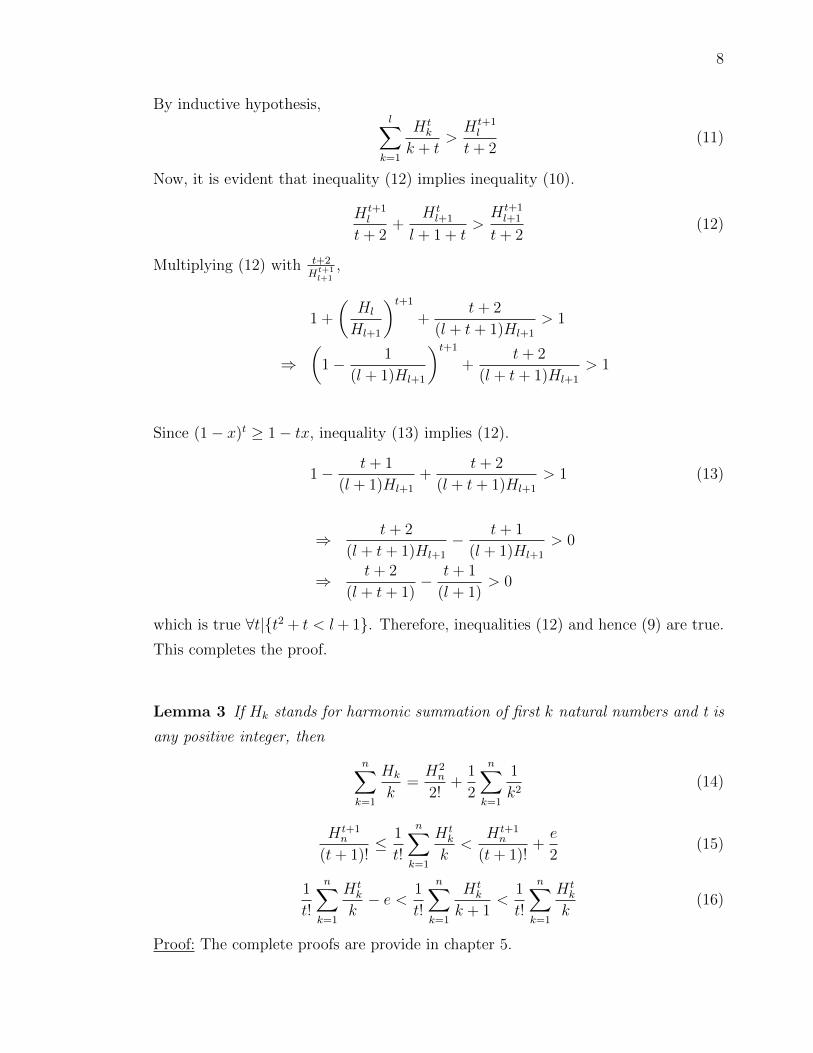
which is true ∀t|{t2 + t < l+ 1}. Therefore, inequalities (12) and hence (9) are true.
This completes the proof.
Lemma 3 If Hk stands for harmonic summation of first k natural numbers and t is
any positive integer, then
n∑k=1
Hk
k=H2n
2!+
1
2
n∑k=1
1
k2(14)
H t+1n
(t+ 1)!≤ 1
t!
n∑k=1
H tk
k<
H t+1n
(t+ 1)!+e
2(15)
1
t!
n∑k=1
H tk
k− e < 1
t!
n∑k=1
H tk
k + 1<
1
t!
n∑k=1
H tk
k(16)
Proof: The complete proofs are provide in chapter 5.

9
III.3 UPPER BOUND (UB) ON PR{L = l}
Lemma 4 The probability that the length of the misparking chain is 2 is bounded
above as represented by inequality (17):
Pr{L = 2} < 1
n− 1
(H2n−1
2!+e
2
)(17)
Proof: Based on the system model, the probablity is given by:
Pr{L = 2} = Pr{Zi}n−1∑i=1
Pr{Ai,j}n∑
j=i+1
Pr{Bj}
which is equivalent to
Pr{L = 2} =1
n− 1
n−1∑i=1
1
n− i
n∑j=i+1
1
n− j + 1
=1
n− 1
n−1∑i=1
Hn−i
n− i
=1
n− 1
n−1∑k=1
Hk
k
=1
n− 1
(H2n−1
2!+
1
2
n−1∑k=1
1
k2
)<
1
n− 1
(H2n−1
2!+e
2
)Using Lemma 3
Lemma 5 The probability that the length of the misparking chain is 3 is bounded
above as represented by inequality (18):
Pr{L = 3} < 1
n− 1
(H3n−2
3!+e
2
)(18)
Proof: Again based on the system model, the probability is given by:
Pr{L = 3} = Pr{Zi}[ n−2∑i=1
Pr{Ai,j}n−1∑j=i+1
Pr{Aj,k}n∑
k=j+1
Pr{Bk}]

10
which is equivalent to
1
n− 1
n−2∑i=1
1
n− i
n−1∑j=i+1
1
n− j + 1
n∑k=j+1
1
n− k + 1
=1
n− 1
n−2∑i=1
1
n− i
n−1∑j=i+1
Hn−j
n− j + 1
=1
n− 1
n−2∑i=1
1
n− i
n−i−1∑k=1
Hk
k + 1
≤ 1
n− 1
n−2∑i=1
1
n− iH2n−i−1
2!Using Lemma 1
=1
n− 1
n−2∑k=1
1
k + 1
H2k
2!
<1
n− 1
(H3n−2
3!+e
2
)Using Lemma 3
The upper bounds for chain lengths 4, 5 and 6 are obtained in a similar fashion.
Lemma 6 The probability that the length of the misparking chain is 4, 5 and 6 are
bounded above as given by inequalities (19), (20) and (21), respectively:
Pr{L = 4} < 1
n− 1
(H4n−3
4!+e
2
)(19)
Pr{L = 5} < 1
n− 1
(H5n−4
5!+e
2
)(20)
Pr{L = 6} < 1
n− 1
(H6n−5
6!+e
2
)(21)
Proof: The proof is similar to that provided in lemmas 4 and 5. The general inequality
representing the upper bound on probability that the length of the misparking chain
is any integer l, l ≥ 2 is formally presented in theorem 1. Note that the expressions
for trivial cases where length is 2 and 3 are already presented in lemmas 4 and 5
respectively.
Theorem 1 (Misparking Chain Length Upper Bound) The probability that
the length of the misparking chain is l is bounded above as represented by inequality
(22):
Pr{L = l} < 1
n− 1
(H ln−l+1
l!+e
2
)(22)

11
Proof: Following a similar approach as in preceding lemmas,
Pr{L = l} = Pr{Zi}[ n−l+1∑
i=1
Pr{Ai,j}n−l∑j=i+1
Pr{Aj,k} . . .n∑
y=x+1
Pr{By}]
(23)
which is equivalent to
Pr{L = l} =1
n− 1
n−l+1∑i=1
1
n− i
n−l∑j=i+1
1
n− j + 1. . .
. . .n−1∑y=z+1
1
n− y + 1
n∑x=y+1
1
n− x+ 1
=1
n− 1
n−l+1∑i=1
1
n− i
n−l∑j=i+1
1
n− j + 1. . .
n−1∑y=z+1
Hn−y
n− y + 1
=1
n− 1
n−l+1∑i=1
1
n− i. . .
n−2∑z=w+1
1
n− z + 1
n−z−1∑p=1
Hp
p+ 1
Using Lemma 1,
≤ 1
n− 1
n−l+1∑i=1
1
n− i
n−l∑j=i+1
1
n− j + 1. . .
n−2∑z=w+1
H2n−z−1
n− z + 1
1
2!
=1
n− 1
n−l+1∑i=1
1
n− i
n−l∑j=i+1
1
n− j + 1. . .
n−w−2∑p=1
H2p
p+ 2
1
2!
......
......
=1
n− 1
n−l+1∑i=1
1
n− iH l−1n−i−(l−2)
(l − 1)!
=1
n− 1
n−l+1∑p=1
1
p+ (l − 2)
H l−1p
(l − 1)!
≤ 1
n− 1
n−l+1∑p=1
1
p
H l−1p
(l − 1)!
<1
n− 1
(H ln−l+1
l!+e
2
)(Using Lemma 3)
(24)
This completes the proof.
12
III.4 LOWER BOUND (LB) ON PR{L = l}
The lower bound on the probabilities can be similarly found with the use of Lemma
2.
Theorem 2 (Misparking Chain Length Lower Bound) The probability that
the length of the misparking chain is l is bounded below as represented by inequality
(25):
Pr{L = l} > 2
n− 1
(H ln−l+1
(l + 1)!
)(25)
Proof: From (24),
Pr{L = l} =1
n− 1
n−l+1∑i=1
1
n− i
n−l∑j=i+1
1
n− j + 1. . .
. . .n−1∑y=z+1
1
n− y + 1
n∑x=y+1
1
n− x+ 1
=1
n− 1
n−l+1∑i=1
1
n− i
n−l∑j=i+1
1
n− j + 1. . .
n−1∑y=z+1
Hn−y
n− y + 1
=1
n− 1
n−l+1∑i=1
1
n− i. . .
n−2∑z=w+1
1
n− z + 1
n−z−1∑p=1
Hp
p+ 1
Using lemma 2,
>2
n− 1
n−l+1∑i=1
1
n− i
n−l∑j=i+1
1
n− j + 1. . .
n−2∑z=w+1
H2n−z−1
n− z + 1
1
3!
=2
n− 1
n−l+1∑i=1
1
n− i
n−l∑j=i+1
1
n− j + 1. . .
n−w−2∑p=1
H2p
p+ 2
1
3!
13
Applying Lemma 2 iteratively in this fashion from right to left, we end up with
Pr{L = l} >2
n− 1
n−l+1∑i=1
1
n− iH l−1n−i−(l−2)
(l)!
=2
n− 1
n−l+1∑p=1
1
p+ (l − 2)
H l−1p
(l)!
>2
n− 1
n−l+1∑p=1
1
p+ (l − 1)
H l−1p
(l)!
>2
n− 1
(H ln−l+1
(l + 1)!
)(Using lemma 2)
This completes the proof.
Combining Theorems 1 and 3,
Theorem 3 (Misparking Chain Length) The probability that the length of the
misparking chain is l is best represented by inequality (26):
2
n− 1
(H ln−l+1
(l + 1)!
)< Pr{L = l} < 1
n− 1
(H ln−l+1
l!+e
2
)(26)
Proof: The result in (26) follows directly from theorems 1 and 3.
III.5 MOST PROBABLE MISPARKING CHAIN LENGTH
In this section, the upperbound on L̂, the most probable chain length is determined.
Inequalities (22) and (25) clearly establish bounds on probabilities of occurence of
different lengths of misparking chain. Higher the difference between the upper and
the lower bound, greater is the probability of occurence of the corresponding chain
length. Let g(l) be the function representing the difference between the bounds given
by (22) and (25) respectively.
g(l) =1
n− 1
(l − 1
l + 1
H ln−l+1
l!+e
2
)(27)
Also let,
f(l) =l − 1
l + 1
H ln−l+1
l!. (28)
Therefore, max(f(l))⇒ max(g(l)).
Also,max(g(l)) = g(L̂).
Let us now study the properties of f(l).
14
Lemma 7
f(l + 1) < f(l),∀l ≥ dHn−le (29)
Proof:
f(l + 1)− f(l) =l
l + 2
H l+1n−l
(l + 1)!− l − 1
l + 1
H ln−l+1
l!
=l − 1
(l + 1)!
(lHn−l
l2 + l − 2H ln−l −H l
n−l+1
)< 0, ∀l ≥ dHn−le, Since 2 ≤ l ≤ n− 1
or equivalently
f(l + 1)− f(l) < 0, ∀l ≥ dHne
(30)
Lemma 7 proves that f(l) is decreasing in the range [dHne,∞], which implies g(l) is
decreasing in the range [dHne,∞]. Since g(L̂) = max(g(l)),
L̂ ≤ dHne (31)
It is a well known fact that Hn = Θ(lnn). Therefore, the most probable chain length
follows a Θ(lnn) order of growth.
III.6 SIMULATION RESULTS
This section presents the analysis based results followed by a camparison of the same
with the results obtained from simulation. The conditions assumed for simulation is
same as those assumed in theoretical analysis. Each of the n available parking slots
is reserved by one of the n drivers. A driver Pi, in the range P1 to Pn is randomly
selected to mispark in a randomly selected slot different from the one reseved by
him/her. The remaining drivers park in their reserved slots if available or else park
in one of the remaining available slots, which also is randomly selected. The length
of the misparking chain is noted when the last driver in the chain parks in the slot
reserved by the first driver to mispark, Pi.
Two different sets of simulation, one with 100000 runs and other with 1000000
runs are performed to compute the probabilities Pr{L = l}, for different values of l.
Let s denote the number of simulation runs. The theoretical bounds together with
simulation results for n = 500,s = 100000 are depicted in Fig. 3. It is observed that

15
FIG. 3: Bounds vs simulation results, n = 500,s = 100000.
the curve representing the actual probability values obtained from simulation peaks
at bHnc − 1 = L̂, the curve representing the theoretical upperbounds obtained from
(22) peaks at bHnc and the curve representing the theoretical lowerbounds obtained
from (25) peaks at bHnc − 1. Thus, L̂ is less than dHne as claimed. It is clearly
visible in Fig. 3 that the simulation based results never exceed the corresponding
bounds. Next, s is increased to 1000000 keeping n constant at 500. Even in this case,
the simulation results do not exceed the corresponding bounds as is evident from
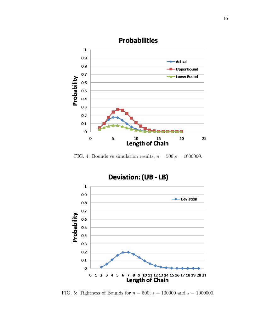
results of Fig. 4. The tightness of the proposed bounds, expressed as the difference
between the upperbound and the lowerbound, is plotted in Fig. 5 for n = 500.
An important observation made in Fig. 5 is that the maximum difference between
the computed bounds is 0.196, which is 19.6% of the maximum possible difference
since the probabilities are trivially bounded between 0 and 1. The average difference
between the proposed bounds for n = 500 is 0.065 or 6.5% of the trivial maximum.
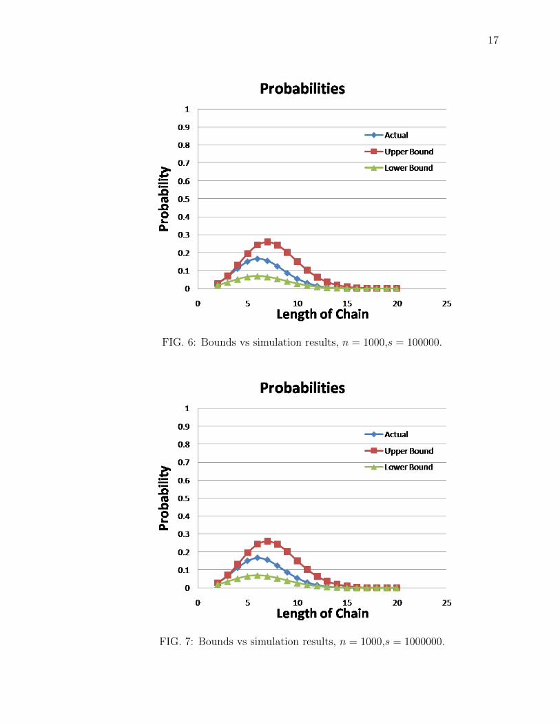
Similar results for n = 1000, n = 5000 are presented next in figures 6, 7, 8. 9, 10 and
11. Even in these scenarios, it is observed that the curve representing the actual
probabilities obtained through simulation peak at bHnc−1, the curve representing the
16
FIG. 4: Bounds vs simulation results, n = 500,s = 1000000.
FIG. 5: Tightness of Bounds for n = 500, s = 100000 and s = 1000000.
17
FIG. 6: Bounds vs simulation results, n = 1000,s = 100000.
FIG. 7: Bounds vs simulation results, n = 1000,s = 1000000.
18
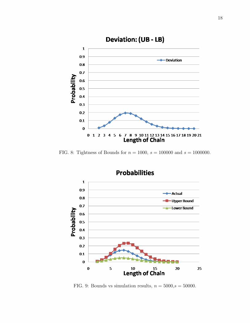
FIG. 8: Tightness of Bounds for n = 1000, s = 100000 and s = 1000000.
FIG. 9: Bounds vs simulation results, n = 5000,s = 50000.

19
FIG. 10: Bounds vs simulation results, n = 1000,s = 100000.
FIG. 11: Tightness of Bounds for n = 5000, s = 50000 and s = 100000.
20
computed upper bound peaks at bHnc, whereas the curve representing the computed
lower bound peaks at bHnc−1. In any case, L̂ ≤ dHne as claimed. The maximum and
average difference between bounds for n = 1000 are 0.195(19.5%) and 0.068(6.8%)
respectively. The maximum and average difference between bounds for n = 5000
are 0.187(18.7%) and 0.073(7.3%) respectively. In each of the above cases, it is
observed that the range of chain lengths having significant probability of occurance
is extremely small compared to the size of the garage. Overall, results depict that
the impact of a mispark on the reservation based parking system is extremely low,
considering the large size n of the parking garage. In other words, the system is
self healing and does not require additional expensive infrastructure, thereby making
reservation a reliable solution to the parking problem in large metros.

21
CHAPTER IV
A RECURSIVE SOLUTION
In this section, a recursive solution is proposed to compute the probability of oc-
curence of any length p of the misparking chain. With the use of this recursive
solution, an approximation to the actual probability is derived.
IV.1 FIRST DRIVER INITIATING MISPARK
Let Bp(N) denote the event that a misparking chain of length p occurs in a garage
of size N , given that the first driver to enter the garage misparks. Using the law of
total probability, we get
Pr{Bp(N)} =N∑j=2
Pr{Bp(N)|{1→ j}}Pr{1→ j} (32)
where p ≥ 3.
Now,
Pr{Bp(N)|{1→ j}} =N − j
N − j + 1Pr{Bp−1(N − j + 1)} (33)
where N−jN−j+1
represents the probability that j does not close the chain. Therefore,
Pr{Bp(N)} =1
N − 1
N∑j=2
N − jN − j + 1
Pr{Bp−1(N − j + 1)} (34)
Taking k = N − j + 1, we get (35).
Pr{Bp(N)} =1
N − 1
N−1∑k=p−1
k − 1
kPr{Bp−1(k)} (35)
since k ≥ p− 1.
Let ap,N = Pr{Bp(N)}. It is known from the previous section that,
a2,N =HN−1
N − 1(36)
Also from (35),
ap,N =1
N − 1
N−1∑k=p−1
k − 1
kap−1,k, p ≥ 3 (37)

22
Now,
ap,N+1 =1
N
N∑k=p−1
k − 1
kap−1,k
=1
N
N−1∑k=p−1
k − 1
kap−1,k +
1
N
N − 1
Nap−1,N ,
Therefore, from (35) and (38),
(N)ap,N+1 = (N − 1)ap,n +N − 1
Nap−1,N (38)
or equivalently,
(N)ap,N+1 − (N − 1)ap,N =N − 1
Nap−1,N , p ≥ 3 (39)
IV.1.1 An Approximate Solution
In this subsection, it is proven that (39) is satisfied by
ap,N =lnp−1(N − 1)
(p− 1)!(N − 1), for largeN. (40)
Some of the results specified in Apendix A are used by the prrofs provided in this
section. Now, LHS of (39) after substituting (40) is given by,
N.lnp−1(N)
(p− 1)!N− (N − 1)
lnp−1(N − 1)
(p− 1)!(N − 1)=
1
(p− 1)!
(lnp−1(N)− lnp−1(N − 1)
)(41)
and RHS is given by,
N − 1
N
lnp−2(N − 1)
(N − 1)(p− 2)!=
lnp−2(N − 1)
(p− 2)!N(42)
The goal is to show that LHS ≈ RHS for large N .
Theorem 4
1
(p− 1)!
(lnp−1(N)− lnp−1(N − 1)
)>
lnp−2(N − 1)
(p− 2)!N(43)
Proof:
To see this, observe that
1
(p− 1)!
(lnp−1(N)− lnp−1(N−1)
)=
1
(p− 1)!ln
(N
N − 1
) p−2∑i=0
lnp−2−i(N) lni(N−1)
(44)

23
by binomial expansion. Now,
1
(p− 1)!
(lnp−1(N)− lnp−1(N − 1)
)− lnp−2(N − 1)
(p− 2)!N
=1
(p− 1)!N
(N. ln
(N
N − 1
) p−2∑i=0
lnp−2−i(N) lni(N − 1)− (p− 1) lnp−2(N − 1)
)
>1
(p− 1)!N
( p−2∑i=0
lnp−2−i(N) lni(N − 1)− (p− 1) lnp−2(N − 1)
)
>1
(p− 1)!N
( p−2∑i=0
lnp−2(N − 1)− (p− 1) lnp−2(N − 1)
)= 0
Hence proved.
Theorem 5
1
(p− 1)!
(lnp−1(N)− lnp−1(N − 1)
)− lnp−2(N − 1)
(p− 2)!N<
1
N − 1(45)
Proof:
Let,
f(p, n) =1
(p− 1)!
(lnp−1(N)− lnp−1(N − 1)
)− lnp−2(N − 1)
(p− 2)!N(46)
=1
(p− 1)!N
(N(lnp−1(N)− lnp−1(N − 1))− (p− 1) lnp−2(N − 1)
)=
1
(p− 1)!N
((N − 1)(lnp−1(N)− lnp−1(N − 1)) + (lnp−1(N)− lnp−1(N − 1))
−(p− 1) lnp−2(N − 1)
)=
1
(p− 1)!N
((N − 1) ln
N
N − 1
p−2∑i=0
lnp−2−i(N). lni(N − 1) + (lnp−1(N)
− lnp−1(N − 1))− (p− 1) lnp−2(N − 1)
)≤ 1
(p− 1)!N
( p−2∑i=0
lnp−2−i(N). lni(N − 1)− (p− 1) lnp−2(N − 1)
+(lnp−1(N)− lnp−1(N − 1))
)(47)

24
Consider,
p−2∑i=0
lnp−2−i(N). lni(N − 1)− (p− 1) lnp−2(N − 1)
=
p−2∑i=0
lni(N − 1)
(lnp−2−i(N)− lnp−2−i(N − 1)
)
=
p−2∑i=0
lni(N − 1) lnN
N − 1
p−3−i∑j=0
lnp−3−i−j N lnj(N − 1)
<1
N − 1
p−2∑i=0
lni(N − 1).(N − 1) ln(N
N − 1)
p−3−i∑j=0
lnp−3−i−j(N) lnj(N)
<1
N − 1
p−2∑i=0
lni(N).(p− 2− i) lnp−3−i(N)
=1
N − 1lnp−3(N)
p−2∑i=0
(p− 2− i)
=1
N − 1
(p− 2)(p− 1)
2lnp−3(N)
<1
N − 1(p− 2)(p− 1) lnp−3(N) (48)
Also,
lnp−1(N)− lnp−1(N − 1) = ln
(N
N − 1
) p−2∑i=0
lnp−2−i(N). lni(N − 1)
<1
N − 1(N − 1) ln
(N
N − 1
).(p− 1) lnp−2(N)
<1
N − 1(p− 1) lnp−2(N)
Substituting (48) and (49) in (47), we get
1
N(N − 1)(p− 1)!
((p− 1)(p− 2) lnp−3N + (p− 1) lnp−2N
)=
1
N(N − 1)
(lnp−3N
(p− 3)!+
lnp−2N
(p− 2)!
)<
1
N(N − 1)elnN
=1
N − 1
Hence proved. Therefore,
0 < LHS −RHS < 1
N − 1(49)

25
FIG. 12: Simulation vs Approximation, n = 1000.
Note that limn→∞
(1
N−1
)= 0. Hence, LHS ≈ RHS for large N .
IV.1.2 Most Probable Chain Length Estimate
The proposed approximate solution lnp−1(N−1)(p−1)!(N−1) is a Poisson probability mass function
with parameter λ = ln(N − 1).
Since, λ is the expected value of a Poisson random variable, the most probable length
of the misparking chain is approximately λ = ln(N − 1).
IV.1.3 Results
In this subsection, the thoretical estimates proposed in the previous subsection are
compared with the actual values obtained from simulation for various garage capac-
ities. The number of simulation runs in all these experiments is one million. The
graphs depicting the results are presented next. It can be observed from the pre-
vious graphs that the approximation is very close to the simulation values. Also, it
can be observed that greater the value of N , better is the approximation. This fact is
depicted in Fig. 16 and Fig. 17. It is clearly seen in Fig. 16 that the curve dampens
towards the x axis with increase in N , thereby indicating that better approximations
are obtained when the size of the garage is large. The average computed in each case

26
FIG. 13: Simulation vs Approximation, n = 3000.
FIG. 14: Simulation vs Approximation, n = 5000.

27
FIG. 15: Simulation vs Approximation, n = 7000.
FIG. 16: Difference between simulation and approximation.

28
FIG. 17: Average difference between simulation and approximation.
is then plotted in Fig. 17. Even in this case, the average error decreases with increase
in N . Also, notice in Fig. 12 that the curve representing simulation result peaks at 7,
indicating that the most probable length of the misparking chain for N = 1000 is 7.
Now, the curve representing the approximation also peaks at ln(1000− 1) = 6.9 ≈ 7,
thereby demonstrating the closeness of the approximation to the simulation result.
Similar observations are made in Fig. 13, Fig. 14 and Fig. 15. The simulation
curves in all these figures peak exactly at corresponding ln(N − 1). Therefore, it
can be inferred that the most probable length of the misparking chain is extremely
small compared to the size of the parking garage. In other words, misparking has
negligible effect on the stability of a reservation based parking system and hence can
be safely ignored while designing parking assistance mechanisms.

29
CHAPTER V
SUMMATION OF TERMS INVOLVING HARMONIC SERIES
In previous chapters, we encountered several complex expressions involving summa-
tions of terms involving harmonic sums. It is very important to determine the exact
closed form equivalents to these terms or atleast good approximations when exact
equivalents do not exist. This chapter deals with analysis of these complex terms.
More specifically, a novel technique is proposed to determine the exact values of
such complex expressions. In addition, certain interesting properties of these expres-
sions are presented which were made use of in probabilistic analysis of misparking
described in earlier chapters.
V.1 COMPUTATION OF∑N
K=1HK
KAND
∑NK=1
H2K
K
First, the value of the expression∑n
k=1Hk
kis computed. The proposed technique
defines a custom matrix like arragement displayed below.
11
12
13
...
1k
...
1n
11
+ 12
+ 13
+ . . .+ 1k
+ . . .+ 1n
12
+ 13
+ . . .+ 1k
+ . . .+ 1n
13
+ . . .+ 1k
+ . . .+ 1n
...
...
1n−1 + 1
n
1n
The above arrangement called Real is considered to be equivalent to the value given
by the expression in (50). For each row of the right matrix, an intermediate value
is generated by mutiplying the summation of all the values in that row with the
corresponding row entry in the single column martix on the left side. The summation

30
of all these intermediate values represents the value of Real.
1
1
n∑k=1
1
k+
1
2
n∑k=2
1
k+ . . .+
1
n∗ 1
n(50)
By rearraging the terms of the above equation, it can be observed that it is equivalent
to (51).n∑k=1
1
k
k∑i=1
1
i=
n∑k=1
Hk
k(51)
The arrangement Real therefore represents∑n
k=1Hk
k. Next, Real is completed by
filling the empty spaces as presented next. Let us refer to the new arrangement as
the Rectangle.
11
12
13
...
1k
...
1n
11
+ 12
+ 13
+ . . .+ 1k
+ . . .+ 1n
11
+ 12
+ 13
+ . . .+ 1k
+ . . .+ 1n
11
+ 12
+ 13
+ . . .+ 1k
+ . . .+ 1n
...
11
+ 12
+ 13
+ . . .+ 1k
+ . . .+ 1n
...
11
+ 12
+ 13
+ . . .+ 1k
+ . . .+ 1n
Following similar lines of interpretation as in Real, the arrangement Rectangle is
considered to be equivalent to (52).
1
1
n∑k=1
1
k+
1
2
n∑k=1
1
k+ . . .+
1
n
n∑k=1
1
k(52)
(52) on simplification yields (53).
n∑k=1
1
k
k∑k=1
1
k= H2
n (53)
The new arrangement Rectangle therefore represents H2n. Another arragement
Lower Triangle consisting of all the terms present in Rectangle but not in Real

31
is defined. The Lower Triangle arrangement is presented next.
12
13
...
1k
...
1n
11
11
+ 12
...
11
+ 12
+ 13
+ . . .+ 1k−1
...
11
+ 12
+ 13
+ . . .+ 1k
+ . . .+ 1n−1
The value corresponding to Lower Triangle is given by (54)
n∑k=2
1
k
k−1∑i=1
1
i=
n∑k=1
Hk
k−
n∑k=1
1
k2(54)
It is evident that the relationship between the three arrangements described previ-
ously is given by
Rectangle=Real+Lower Triangle
or equivalently,
Real=Rectangle-Lower Triangle.
Therefore,n∑k=1
Hk
k= H2
n −n∑k=1
Hk
k+
n∑k=1
1
k2(55)
which on simplification yields (56).
n∑k=1
Hk
k=
1
2H2n +
1
2
n∑k=1
1
k2(56)
(56) provides an expression to determine the exact value of∑n
k=1Hk
kFollowing a
similar approach, the expression∑n
k=1
H2k
kis evaluated. The Real arrangement to

32
evaluate∑n
k=1
H2k
kis shown below.
11
12
13
...
1k
...
1n
H1
1+ H2
2+ H3
3+ . . .+ Hk
k+ . . .+ Hn
n
H2
2+ H3
3+ . . .+ Hk
k+ . . .+ Hn
n
H3
3+ . . .+ Hk
k+ . . .+ Hn
n
...
...
Hn−1
n−1 + Hn
n
Hn
n
Following a procedure similar to that used in evaluating
∑nk=1
Hk
k, the following set
of equations are obtained.
Real =n∑k=1
H2k
k(57)
Rectangle =n∑k=1
1
k
n∑k=1
Hk
k=
1
2H3n +
1
2Hn
n∑k=1
1
k2(58)
Lower Triangle =n∑k=2
1
k
k−1∑i=1
Hi
i=
1
2
n∑k=1
H2k
k+
1
2
n∑k=1
1
k
k∑i=1
1
i2−
n∑k=1
Hk
k2(59)
Again, since Real = Rectangle - Lower Triangle,
n∑k=1
H2k
k=
1
2H3n +
1
2Hn
n∑k=1
1
k2− 1
2
n∑k=1
H2k
k− 1
2
n∑k=1
1
k
k∑i=1
1
i2+
n∑k=1
Hk
k2(60)
which on simplification yields (61),
n∑k=1
H2k
k=
1
3H3n +
1
3Hn
n∑k=1
1
k2− 1
3
n∑k=1
1
k
k∑i=1
1
i2+
2
3
n∑k=1
Hk
k2(61)
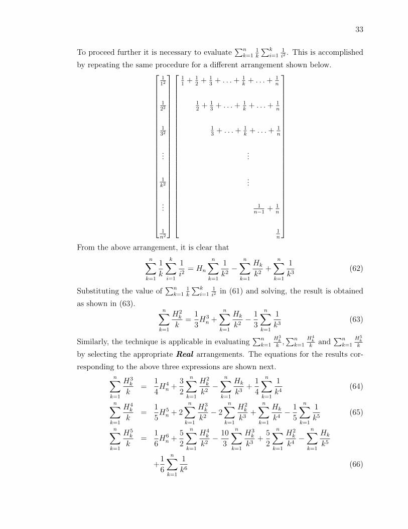
33
To proceed further it is necessary to evaluate∑n
k=11k
∑ki=1
1i2
. This is accomplished
by repeating the same procedure for a different arrangement shown below.
112
122
132
...
1k2
...
1n2
11
+ 12
+ 13
+ . . .+ 1k
+ . . .+ 1n
12
+ 13
+ . . .+ 1k
+ . . .+ 1n
13
+ . . .+ 1k
+ . . .+ 1n
...
...
1n−1 + 1
n
1n
From the above arrangement, it is clear that
n∑k=1
1
k
k∑i=1
1
i2= Hn
n∑k=1
1
k2−
n∑k=1
Hk
k2+
n∑k=1
1
k3(62)
Substituting the value of∑n
k=11k
∑ki=1
1i2
in (61) and solving, the result is obtained
as shown in (63).n∑k=1
H2k
k=
1
3H3n +
n∑k=1
Hk
k2− 1
3
n∑k=1
1
k3(63)
Similarly, the technique is applicable in evaluating∑n
k=1
H3k
k,∑n
k=1
H4k
kand
∑nk=1
H5k
k
by selecting the appropriate Real arrangements. The equations for the results cor-
responding to the above three expressions are shown next.n∑k=1
H3k
k=
1
4H4n +
3
2
n∑k=1
H2k
k2−
n∑k=1
Hk
k3+
1
4
n∑k=1
1
k4(64)
n∑k=1
H4k
k=
1
5H5n + 2
n∑k=1
H3k
k2− 2
n∑k=1
H2k
k3+
n∑k=1
Hk
k4− 1
5
n∑k=1
1
k5(65)
n∑k=1
H5k
k=
1
6H6n +
5
2
n∑k=1
H4k
k2− 10
3
n∑k=1
H3k
k3+
5
2
n∑k=1
H2k
k4−
n∑k=1
Hk
k5
+1
6
n∑k=1
1
k6(66)

34
V.2 COMPTUTATION OF∑N
K=1HP
K
K,P > 0
Next, a general equation to compute∑n
k=1
Hpk
k, p > 0 is determined.
Lemma 8
n∑k=1
Hpk
k= a0(p)H
p+1n + a1(p)
n∑k=1
Hp−1k
k2+ a2(p)
n∑k=1
Hp−2k
k3+ . . .+ ap(p)
n∑k=1
1
kp+1(67)
with the condition that∑p
i=0 ai(p) = 1.
Proof: By induction on p.
Base case: With reference to earlier derivations, the above hypothesis is easy verified
for the base case p = 1.
Inductive step: Using the same procedure as before the value of∑n
k=1
Hp+1k
kis deter-
mined using an arrangement shown below.
11
12
13
...
1k
...
1n
Hp1
1+
Hp2
2+
Hp3
3+ . . .+
Hpk
k+ . . .+ Hp
n
n
Hp2
2+
Hp3
3+ . . .+
Hpk
k+ . . .+ Hp
n
n
Hp3
3+ . . .+
Hpk
k+ . . .+ Hp
n
n
...
...
Hpn−1
n−1 + Hpn
n
Hpn
n
35
With respect to the arrangement shown above, the following set of equations are
obtained.
Real =n∑k=1
Hp+1k
k(68)
Rectangle = Hn
n∑k=1
Hpk
k(69)
Lower triangle =n∑k=1
1
k
k∑i=1
Hpi
i−
n∑k=1
Hpk
k2(70)
Therefore,n∑k=1
Hp+1k
k= Hn
n∑k=1
Hpk
k−
n∑k=1
1
k
k∑i=1
Hpi
i+
n∑k=1
Hpk
k2(71)
By inductive hypothesis, substituting the values of∑n
k=1
Hpk
kand
∑ki=1
Hpi
iin equation
(71),n∑k=1
Hp+1k
k= Hn
[a0(p)H
p+1n + a1(p)
n∑k=1
Hp−1k
k2+ a2(p)
n∑k=1
Hp−2k
k3+ . . .
+ap(p)n∑k=1
1
kp+1
]−
n∑k=1
1
k
[a0(p)H
p+1k + a1(p)
k∑i=1
Hp−1i
i2
+a2(p)k∑i=1
Hp−2i
i3+ . . .+ ap(p)
k∑i=1
1
ip+1
]+
n∑k=1
Hpk
k2
which implies,n∑k=1
Hp+1k
k= a0(p)H
p+2n + a1(p)Hn
n∑k=1
Hp−1k
k2+ a2(p)Hn
n∑k=1
Hp−2k
k3+ . . .
+ap(p)Hn
n∑k=1
1
kp+1− a0(p)
n∑k=1
Hp+1k
k− a1(p)
n∑k=1
1
k
k∑i=1
Hp−1i
i2
−a2(p)n∑k=1
1
k
k∑i=1
Hp−2i
i3− . . .− ap(p)
n∑k=1
1
k
k∑i=1
1
ip+1+
n∑k=1
Hpk
k2
which on simplification gives,[1 + a0(p)
] n∑k=1
Hp+1k
k= a0(p)H
p+2n + a1(p)
[Hn
n∑k=1
Hp−1k
k2−
n∑k=1
1
k
k∑i=1
Hp−1i
i2
]
+a2(p)
[Hn
n∑k=1
Hp−2k
k3−
n∑k=1
1
k
k∑i=1
Hp−2i
i3
]+ . . .
+ap(p)
[Hn
n∑k=1
1
kp+1−
n∑k=1
1
k
k∑i=1
1
ip+1
]+
n∑k=1
Hpk
k2

36
Let,
αj(n) = Hn
n∑k=1
Hp−jk
kj+1−
n∑k=1
1
k
k∑i=1
Hp−ji
ij+1(72)
It is clearly evident that αj(p) = 0.
Therefore,
αj(n+ 1) = Hn+1
n+1∑k=1
Hp−jk
kj+1−
n+1∑k=1
1
k
k∑i=1
Hp−ji
ij+1
=
[Hn +
1
n+ 1
][ n∑k=1
Hp−jk
kj+1+
Hp−jn+1
(n+ 1)j+1
]
−n∑k=1
1
k
k∑i=1
Hp−ji
ij+1− 1
n+ 1
n+1∑i=1
Hp−ji
ij+1
=
[Hn
n∑k=1
Hp−jk
kj+1−
n∑k=1
1
k
k∑i=1
Hp−ji
ij+1
]+
HnHp−jn+1
(n+ 1)j+1
+1
n+ 1
n+1∑k=1
Hp−jk
kj+1− 1
n+ 1
n+1∑i=1
Hp−ji
ij+1
= αj(n) +
[Hn+1 − 1
n+1
]Hp−jn+1
(n+ 1)j+1
= αj(n) +Hp−j+1n+1
(n+ 1)j+1−
Hp−jn+1
(n+ 1)j+2
On solving the recurrence,
αj(n) =n∑k=1
Hp−j+1k
kj+1−
n∑k=1
Hp−jk
kj+2(73)

37
Therefore,[1 + a0(p)
] n∑k=1
Hp+1k
k= a0(p)H
p+2n +
n∑k=1
Hpk
k2+ a1(p)
[ n∑k=1
Hpk
k2−
n∑k=1
Hp−1k
k3
]+a2(p)
[ n∑k=1
Hp−1k
k3−
n∑k=1
Hp−2k
k4
]+ a3(p)
[ n∑k=1
Hp−2k
k4
−n∑k=1
Hp−3k
k5
]+ . . .+ ap(p)
[ n∑k=1
Hk
kp+1−
n∑k=1
1
kp+2
]= a0(p)H
p+2n +
[1 + a1(p)
] n∑k=1
Hpk
k2+
[a2(p)
−a1(p)] n∑k=1
Hp−1k
k3+ . . .+
[ap(p)− ap−1(p)
] n∑k=1
Hk
kp+1
−ap(p)n∑k=1
1
kp+2
Hence,
n∑k=1
Hp+1k
k=
a0(p)
1 + a0(p)Hp+2n +
1 + a1(p)
1 + a0(p)
n∑k=1
Hpk
k2
+a2(p)− a1(p)
1 + a0(p)
n∑k=1
Hp−1k
k3+ . . .+
ap(p)− ap−1(p)1 + a0(p)
n∑k=1
Hk
kp+1
− ap(p)
1 + a0(p)
n∑k=1
1
kp+2
The coefficients are a0(p)1+a0(p)
,1+a1(p)1+a0(p)
,a2(p)−a1(p)1+a0(p)
,ap(p)−ap−1(p)
1+a0(p),. . . and − ap(p)
1+a0(p).
It can be easily verified that sum of coefficients is 1.
This completes the proof.
V.2.1 Evaluating Coefficients
In this section, a closed form solution for evaluating the coefficients ai(p), 0 ≤ i ≤ p
used in the previous section is provided.
The known values of ai(p), 0 ≤ i ≤ p as shown below are analyzed to frame a general

38
closed form solution for ai(p).
p = 1
p = 2
p = 3
a0(p) a1(p) a2(p) a3(p) . . .
12
12
13
1 − 13
14
32− 1 1
4
The analysis begins with a0(p).
Lemma 9
a0(p) =1
p+ 1(74)
Proof: From the derivations in the preceding section, it is known that a0(p + 1) =a0(p)
1+a0(p)If a0(p) = 1
p+1, then a0(p+ 1) =
1p+1p+2p+1
= 1p+2
.
Hence proved.
Lemma 10
a1(p) =p
2(75)
Proof: Again, a1(p+1) = 1+a1(p)1+a0(p)
If a0(p) = 1p+1
, a1(p) = p2, then a1(p+1) =
p+22
p+2p+1
= p+12
.
Hence proved.
Following similar lines for proofs, the following solutions are obtained for coefficients
a2(p), a3(p)anda4(p).
a2(p) = −p(p− 1)
6= −p(p− 1)
3!= −1
3
(p
2
)a3(p) =
p(p− 1)(p− 2)
4!=
1
4
(p
3
)a4(p) = −1
5
(p
4
)In general,
aj(p) = (−1)j+1 1
j + 1
(p
j
). (76)

39
It is required to verify that,p∑j=1
aj(p) =p
p+ 1. (77)
p∑j=1
(−1)j+1 1
j + 1
(p
j
)=
p∑j=1
(−1)j+1 1
p+ 1
(p+ 1
j + 1
)
=1
p+ 1
p∑j=1
(−1)j+1
(p+ 1
j + 1
)
=1
p+ 1
p+1∑k=2
(−1)k(p+ 1
k
)
=1
p+ 1
[ p+1∑k=0
(−1)k(p+ 1
k
)− 1 + (p+ 1)
]=
1
p+ 1
[0− 1
p+ 1+ 1
]=
p
p+ 1
Hence the claim. Also,
aj(p+ 1) =(−1)j+1 1
j+1
(pj
)− (−1)j 1
j
(pj−1
)p+2p+1
= (−1)j+1p+ 1
p+ 2
[1
j + 1
(p
j
)+
1
j
(p
j − 1
)]= (−1)j+1p+ 1
p+ 2
1
j + 1
[(p
j
)+j + 1
j
(p
j − 1
)]= (−1)j+1p+ 1
p+ 2
1
j + 1
[(p
j
)+
(p
j − 1
)+
1
j
(p
j − 1
)]= (−1)j+1p+ 1
p+ 2
1
j + 1
[(p+ 1
j
)+
1
p+ 1
p+ 1
j
(p
j − 1
)]= (−1)j+1p+ 1
p+ 2
1
j + 1
[(p+ 1
j
)+
1
p+ 1
(p+ 1
j
)]= (−1)j+1p+ 1
p+ 2
1
j + 1
(p+ 1
j
)[1 +
1
p+ 1
]= (−1)j+1 1
j + 1
(p+ 1
j
).
The previous derivation shows that
aj(p) = (−1)j+1 1
j + 1
(p
j
), 1 ≤ j ≤ p (78)

40
Using the above derivations, (67) can be rewritten as (79).
n∑k=1
Hpk
k=Hp+1n
p+ 1+
p∑j=1
(−1)j+1 1
j + 1
(p
j
) n∑k=1
Hp−jk
kj+1(79)
(79) can be further simplified to (80).
n∑k=1
Hpk
k=
1
p+ 1
[Hp+1n +
p∑j=1
(−1)j+1
(p+ 1
j + 1
) n∑k=1
Hp−jk
kj+1
](80)
V.3 PROPERTIES OF∑N
K=1HP
K
K
Some of the interesting properties of∑n
k=1
Hpk
kare highlighted in this section.
Lemma 11n∑k=1
Hpk
k≥ 1
p+ 1Hp+1n (81)
Proof: By induction on n.
Base case: For n = 1, we get Hp1 = 1 ≥ 1
p+1Hp+1
1 = 1p+1
, which is true for all p ≥ 0.
Inductive step: Let the hypothesis be true for any arbitrary integer n.
It has to be proved thatn+1∑k=1
Hpk
k≥ 1
p+ 1Hp+1n+1. (82)
Now,n+1∑k=1
Hpk
k=
n∑k=1
Hpk
k+
Hpn
n+ 1≥ Hp+1
n
p+ 1+
Hpn
n+ 1. (83)
It follows that (82) is established as soon as it is proven that
Hp+1n
p+ 1+
Hpn
n+ 1≥ 1
p+ 1Hp+1n+1. (84)
Multiplying (84) by p+1
Hp+1n+1
, we get
(Hn
Hn+1
)p+1
+p+ 1
n+ 1.
1
Hn+1
≥ 1
=>
(Hn+1 − 1
n+1
Hn+1
)p+1
+p+ 1
n+ 1.
1
Hn+1
≥ 1
=>
(1− 1
(n+ 1)Hn+1
)p+1
+p+ 1
n+ 1.
1
Hn+1
≥ 1

41
It is straightforward to show that
(1− x)n ≥ 1− nx,∀xεR, nεN (85)
With the above inequality (85),(1− 1
(n+ 1)Hn+1
)p+1
+p+ 1
n+ 1.
1
Hn+1
≥ 1− p+ 1
n+ 1.
1
Hn+1
+p+ 1
n+ 1.
1
Hn+1
≥ 1
This completes the proof. The above result clearly shows that the tail of (79) is
greater than 0. That is,
p∑j=1
(−1)j+1 1
j + 1
(p
j
) n∑k=1
Hp−jk
kj+1≥ 0. (86)
Next an upper bound for the tail is established. In order to establish an upper bound
for the tail the following claims are put forth.
Claim 1:
(1− x)n ≤ 1− nx+n(n− 1)
2x2, 0 ≤ x ≤ 1, n ≥ 1 (87)
Proof:
Proof for Claim 1 is provided by induction next.
Basis: It is staightforward that the inequality holds when n = 1.
Inductive step:
Let n be any arbitrary integer for which the hypothesis holds. It is to be shown that,
(1− x)n+1 ≤ 1− (n+ 1)x+n(n+ 1)
2x2, 0 ≤ x ≤ 1, n ≥ 1. (88)
Now,
(1− x)n+1 = (1− x)(1− x)n ≤ (1− x)
(1− nx+
n(n− 1)
2x2)
= 1− nx+n(n− 1)
2x2 − x+ nx2 − n(n− 1)
2x3
= 1− (n+ 1)x+n(n+ 1)
2x2 − n(n− 1)
2x3
≤ 1− (n+ 1)x+n(n+ 1)
2x2

42
Hence proved. Let the tail of (79) be represented as shown in (89).
T (n, p) =1
p+ 1
p+1∑i=2
(−1)i(p+ 1
i
) n∑k=1
Hp+1−ik
ki(89)
Claim 2:
T (n, p)− T (n− 1, p) ≤ p
2
Hp−1n
n2(90)
Proof:
T (n, p)− T (n− 1, p) =1
p+ 1
p+1∑i=2
(−1)i(p+ 1
i
)Hp+1−in
ni
=1
p+ 1
[ p+1∑i=0
(−1)i(p+ 1
i
)Hp+1−in
ni−Hp+1
n + (p+ 1)Hpn
n
]=
1
p+ 1
[(Hn −
1
n
)p+1
−Hp+1n + (p+ 1)
Hpn
n
]=
Hp+1n
p+ 1
[(1− 1
nHn
)p+1
− 1 + (p+ 1)1
nHn
]≤ Hp+1
n
p+ 1
[1− p+ 1
nHn
+p(p+ 1)
2
1
n2H2n
− 1 +p+ 1
nHn
]=
p
2
Hp−1n
n2
Hence the proof.
By Claim 2 we have
T (n, p)− T (n− 1, p) ≤ p
2
Hp−1n
n2
T (n− 1, p)− T (n− 2, p) ≤ p
2
Hp−1n−1
(n− 1)2
T (n− 2, p)− T (n− 3, p) ≤ p
2
Hp−1n−2
(n− 2)2
...
T (2, p)− T (1, p) ≤ p
2
Hp−12
22
It is known that T (1, p) = pp+1
. Summing up the above equations, we get
T (n, p)− T (1, p) ≤ p
2
n∑k=2
Hp−1k
k2. (91)
43
It follows that
T (n, p) ≤ p
p+ 1+
n∑k=2
Hp−1k
k2
≤ p
p+ 1+
n∑k=1
Hp−1k
k2− p
2
≤ p
2
[ n∑k=1
Hp−1k
k2− 1− p
1 + p
]≤ p
2
[ n∑k=1
Hp−1k
k2
]In one of the subsequent derivations, it is shown that
n∑k=1
Hp−1k
k2< e.(p− 1)!. (92)
Therefore,
T (n, p) <e.p!
2. (93)
Or equivalently,T (n, p)
p!<e
2. (94)
Theorem 1 represents the consolidated view of the above results.
Theorem 6Hp+1n
(p+ 1)!≤ 1
p!
n∑k=1
Hpk
k<
Hp+1n
(p+ 1)!+e
2(95)
Next, bounds for 1p!
∑nk=1
Hpk
k+1are established.
Let,
T (n, p) =1
p!
( n∑k=1
Hpk
k−
n∑k=1
Hpk
k + 1
)=
1
p!
n∑k=1
Hpk
k(k + 1)
<1
p!
n∑k=1
Hpk
k2
<1
p!
∫ n
k=1
Hpk
k2dt
44
Now consider∫ nk=1
Hpk
k2dt. On integration by substitution, taking ln k + 1 = t, we get∫ n
k=1
Hpk
k2dt =
∫ lnn+1
t=1
tpe1−tdt
= e
∫ lnn+1
t=1
tpe−tdt
Therefore,
T (n, p) <e
p!
∫ lnn+1
t=1
tpe−tdt. (96)
Also let,
α(p) =
∫ lnn+1
t=1
tpe−tdt
=1
e− (lnn+ 1)p
en+ p.α(p− 1)
α(1) =2
e− lnn+ 1
en− 1
en
Therefore,
α(p) =1
e+p
e+p(p− 1)
e+ . . .+
p!
e
−(
(lnn+ 1)p
en+p(lnn+ 1)p−1
en+p(p− 1)(lnn+ 1)p−2
en
+ . . .+p!(lnn+ 1)
en+
1
en
)<
1
e
(1 + p+ p(p− 1) + . . .+ p!
)<
p!
e
(1
p!+
1
(p− 1)!+ . . .+ 1
)<
p!
e
( p∑i=1
1
i!
)<
p!
e
( ∞∑i=1
1
i!
)<
p!
ee
< p!
Substituting the value of α(p) in (96), we get
T (n, p) <e
p!p! = e (97)

45
The above observations are formally stated in theorem 2 presented next.
Theorem 71
p!
n∑k=1
Hpk
k− e < 1
p!
n∑k=1
Hpk
k + 1<
1
p!
n∑k=1
Hpk
k(98)
Proof: The proofs directly follow from the above dervied results.

46
CHAPTER VI
CONCLUSION
The work in this thesis is directed towards mathematically proving that any reser-
vation based parking system is capable of self recovery with respect to misparking
and that the instability caused by a single mispark is negligible considering the large
capacity of the parking garage. In other words, it is shown both theoretically and
experimentally that the most likely value of length of the chain resulting from a single
mispark follows a Θ(lnn) order of growth which is very small compared to garage
capacity n. First, tight bounds for the probability of misparking chain length are
established. Using these bounds, the behavior of the most probable misparking chain
length is studied. The simulation results clearly agree with the theoretical solutions.
As a next step, a recursive solution is proposed. Then, based on the proposed re-
cursive solution, an approximate solution is proposed. The validity and accuracy of
the approximation is demonstrated through results obtained from both theory and
simulation. In all the experiments, the misparking chain length obtained is extremely
small compared to the size of the parking garage. All the analyses made in this work
are applicable to any reservation based parking system in general. Tighter bounds,
multiple misparks, misparking prevention and design of recovery mechanisms are
scope of future work.
47
BIBLIOGRAPHY
[1] V. Tang, Y. Zheng and J. Cao, An Intelligent Car Park Management Sys-
tem Based on Wireless Sensor Networks, in Proceedings Int. Sym. Pervasive
Computing and Application, Urumqi, pp. 65-70, 2006.
[2] Y. Asakura and M. Kashiwadani, Effects of Parking Availability Information
on System Performance: A Simulation Model Approach, in Proceedings of
Vehicle Navigation and Information System Conference, Dearborn, MI, pp.
251-254, Aug 1994.
[3] B.J. Watterson, N.B. Hounsell and K. Chatterjee, Quantifying the Potential
Savings in Travel Time Resulting from Parking Guidance Systems-A Simu-
lation Case Study, in Journal of the Operational Research Society, Vol. 52,
pp. 1067-1077, 2001.
[4] G.N. Havinoviski, R.V. Taylor, A. Johnston and J.C. Kopp, Real-Time Park-
ing Management Systems for Park-and-Ride Facilities along Transit Corri-
dors, Preprint, Transportation Research Board Annual Meeting, Washington
D.C, 2000.
[5] M.M. Minderhoud and P.H.L. Bovy, A Dynamic Parking Reservation System
for City Centers, in 29th International Symposium on Automotive Technol-
ogy and Automation, pp. 89-96, 1996.
[6] C.R. Cassady and J.E. Kobza, A Probabilistic Approach to Evaluate Strate-
gies for Selecting a Parking Space, in Transportation Science, Vol. 32, No.
1, pp. 30-42, 1998.
[7] R. Panayappan, J.M. Trivedi, A. Studer and A. Perrig, Vanet-based Ap-
proach for Parking Space Availability, in VANET ’07: Proceedings of the
Fourth ACM International Workshop on Vehicular Ad-hoc Networks, New
York, NY, USA, pp. 75-76, 2007.
[8] J. Wolff, T. Heuer, H. Gao, M. Weinmann S. Voit and U. Hartmann, Parking
Monitor System Based on Magnetic Field Sensors, in Proceedings of IEEE
Conf. Intelligent Transport Systems, Toronto, CA, pp. 1275-1279, 2006.

48
[9] R.G. Thompson, P. Bonsall, Driver’s Response to Parking Guidance and
Information Systems, in Transport Reviews, Vol. 17, No. 2, pp. 89-104, 1997.
[10] K.W. Axhausen and J.W. Polak, A dissagregate model of the effects of
parking guidance systems, in 7th WCTR Meeting, topic 9, Advanced Traveler
Information Systems, 1996.
[11] Y. Asakura, M. Kashiwadani, K. Nishi and H. Furuya, Driver’s Response
to Parking Information Systems: Emperical Study in Matuyama City, in
Proceedings of World Congress on Intelligent Transport Systems, Steps For-
ward, Vol. 4, Tokyo, Japan: WERTIS, pp. 1813-1818, 1995.
[12] G. Yan, M.C. Wiegle and S. Olariu, A novel parking service using wireless
networks, IEEE/INFORMS International Conference on Service Operations,
Logistics and informatics, SOLI 2009.
49
APPENDIX A
REVIEW OF SOME IMPORTANT FORMULAE
A.1 EX
ex = 1 +x
1!+x2
2!+x3
3!+ . . . (99)
Therefore,
N = eln(N) = 1 +ln(N)
1!+
(ln(N))2
2!+
(ln(N))3
3!+ . . . (100)
A.2 AN −BN
an − bn = (a− b)n−1∑i=0
an−1−ibi (101)
A.3 LIMITS
limn→∞
(1 +
1
n
)n= e
limn→∞
(1 +
1
n
)n+1
= e
Therefore,
(n− 1) ln
(n
n− 1
)= (n− 1) ln
(1 +
1
n− 1
)= ln
(1 +
1
n− 1
)n−1< ln(e) = 1
(n) ln
(n
n− 1
)= (n− 1 + 1) ln
(1 +
1
n− 1
)= ln
(1 +
1
n− 1
)n−1+1
> ln(e) = 1
A.4 POISSON RANDOM VARIABLE
For a given Poisson random variable X, the probability mass function p is given by,
p(x, λ) =e−λλx
x!(102)
where λ is expected value of X.
50
VITA
Vikas G Ashok
Department of Computer Science
Old Dominion University
Norfolk, VA 23529
EDUCATION
M.S in Computer Science (Present)
Old Dominion University
B.E in Computer Science
Visveswaraiah Technological University, July 2009
Typeset using LATEX.