A Primer on Neural Network Modelsfor Natural Language Processing

Yoav GoldbergDraft as of October 5, 2015.

The most up-to-date version of this manuscript is available at http://www.cs.biu.ac.il/˜yogo/nnlp.pdf. Major updates will be published on arxiv periodically.I welcome any comments you may have regarding the content and presentation. If youspot a missing reference or have relevant work you’d like to see mentioned, do let me know.first.last@gmail

Abstract

Over the past few years, neural networks have re-emerged as powerful machine-learningmodels, yielding state-of-the-art results in fields such as image recognition and speechprocessing. More recently, neural network models started to be applied also to textualnatural language signals, again with very promising results. This tutorial surveys neuralnetwork models from the perspective of natural language processing research, in an attemptto bring natural-language researchers up to speed with the neural techniques. The tutorialcovers input encoding for natural language tasks, feed-forward networks, convolutionalnetworks, recurrent networks and recursive networks, as well as the computation graphabstraction for automatic gradient computation.

1. Introduction

For a long time, core NLP techniques were dominated by machine-learning approaches thatused linear models such as support vector machines or logistic regression, trained over veryhigh dimensional yet very sparse feature vectors.

Recently, the field has seen some success in switching from such linear models oversparse inputs to non-linear neural-network models over dense inputs. While most of theneural network techniques are easy to apply, sometimes as almost drop-in replacements ofthe old linear classifiers, there is in many cases a strong barrier of entry. In this tutorial Iattempt to provide NLP practitioners (as well as newcomers) with the basic background,jargon, tools and methodology that will allow them to understand the principles behindthe neural network models and apply them to their own work. This tutorial is expectedto be self-contained, while presenting the different approaches under a unified notation andframework. It repeats a lot of material which is available elsewhere. It also points toexternal sources for more advanced topics when appropriate.

This primer is not intended as a comprehensive resource for those that will go on anddevelop the next advances in neural-network machinery (though it may serve as a good entrypoint). Rather, it is aimed at those readers who are interested in taking the existing, usefultechnology and applying it in useful and creative ways to their favourite NLP problems. Formore in-depth, general discussion of neural networks, the theory behind them, advanced

1

optimization methods and other advanced topics, the reader is referred to other existingresources. In particular, the book by Bengio et al (2015) is highly recommended.

Scope The focus is on applications of neural networks to language processing tasks. How-ever, some subareas of language processing with neural networks were decidedly left out ofscope of this tutorial. These include the vast literature of language modeling and acousticmodeling, the use of neural networks for machine translation, and multi-modal applicationscombining language and other signals such as images and videos (e.g. caption generation).Caching methods for efficient runtime performance, methods for efficient training with largeoutput vocabularies and attention models are also not discussed. Word embeddings are dis-cussed only to the extent that is needed to understand in order to use them as inputs forother models. Other unsupervised approaches, including autoencoders and recursive au-toencoders, also fall out of scope. While some applications of neural networks for languagemodeling and machine translation are mentioned in the text, their treatment is by no meanscomprehensive.

A Note on Terminology The word “feature” is used to refer to a concrete, linguisticinput such as a word, a suffix, or a part-of-speech tag. For example, in a first-order part-of-speech tagger, the features might be “current word, previous word, next word, previouspart of speech”. The term “input vector” is used to refer to the actual input that is fedto the neural-network classifier. Similarly, “input vector entry” refers to a specific valueof the input. This is in contrast to a lot of the neural networks literature in which theword “feature” is overloaded between the two uses, and is used primarily to refer to aninput-vector entry.

Mathematical Notation I use bold upper case letters to represent matrices (X, Y,Z), and bold lower-case letters to represent vectors (b). When there are series of relatedmatrices and vectors (for example, where each matrix corresponds to a different layer inthe network), superscript indices are used (W1, W2). For the rare cases in which we wantindicate the power of a matrix or a vector, a pair of brackets is added around the item tobe exponentiated: (W)2, (W3)2. Unless otherwise stated, vectors are assumed to be rowvectors. We use [v1; v2] to denote vector concatenation.

2

2. Neural Network Architectures

Neural networks are powerful learning models. We will discuss two kinds of neural networkarchitectures, that can be mixed and matched – feed-forward networks and Recurrent /Recursive networks. Feed-forward networks include networks with fully connected layers,such as the multi-layer perceptron, as well as networks with convolutional and poolinglayers. All of the networks act as classifiers, but each with different strengths.

Fully connected feed-forward neural networks (Section 4) are non-linear learners thatcan, for the most part, be used as a drop-in replacement wherever a linear learner is used.This includes binary and multiclass classification problems, as well as more complex struc-tured prediction problems (Section 8). The non-linearity of the network, as well as theability to easily integrate pre-trained word embeddings, often lead to superior classificationaccuracy. A series of works (Chen & Manning, 2014; Weiss, Alberti, Collins, & Petrov,2015; Pei, Ge, & Chang, 2015; Durrett & Klein, 2015) managed to obtain improved syntac-tic parsing results by simply replacing the linear model of a parser with a fully connectedfeed-forward network. Straight-forward applications of a feed-forward network as a classi-fier replacement (usually coupled with the use of pre-trained word vectors) provide benefitsalso for CCG supertagging (Lewis & Steedman, 2014), dialog state tracking (Henderson,Thomson, & Young, 2013), pre-ordering for statistical machine translation (de Gispert,Iglesias, & Byrne, 2015) and language modeling (Bengio, Ducharme, Vincent, & Janvin,2003; Vaswani, Zhao, Fossum, & Chiang, 2013). Iyyer et al (2015) demonstrate that multi-layer feed-forward networks can provide competitive results on sentiment classification andfactoid question answering.

Networks with convolutional and pooling layers (Section 9) are useful for classificationtasks in which we expect to find strong local clues regarding class membership, but theseclues can appear in different places in the input. For example, in a document classificationtask, a single key phrase (or an ngram) can help in determining the topic of the document(Johnson & Zhang, 2015). We would like to learn that certain sequences of words are goodindicators of the topic, and do not necessarily care where they appear in the document.Convolutional and pooling layers allow the model to learn to find such local indicators,regardless of their position. Convolutional and pooling architecture show promising resultson many tasks, including document classification (Johnson & Zhang, 2015), short-text cat-egorization (Wang, Xu, Xu, Liu, Zhang, Wang, & Hao, 2015a), sentiment classification(Kalchbrenner, Grefenstette, & Blunsom, 2014; Kim, 2014), relation type classification be-tween entities (Zeng, Liu, Lai, Zhou, & Zhao, 2014; dos Santos, Xiang, & Zhou, 2015), eventdetection (Chen, Xu, Liu, Zeng, & Zhao, 2015; Nguyen & Grishman, 2015), paraphrase iden-tification (Yin & Schutze, 2015) semantic role labeling (Collobert, Weston, Bottou, Karlen,Kavukcuoglu, & Kuksa, 2011), question answering (Dong, Wei, Zhou, & Xu, 2015), predict-ing box-office revenues of movies based on critic reviews (Bitvai & Cohn, 2015) modelingtext interestingness (Gao, Pantel, Gamon, He, & Deng, 2014), and modeling the relationbetween character-sequences and part-of-speech tags (Santos & Zadrozny, 2014).

In natural language we often work with structured data of arbitrary sizes, such assequences and trees. We would like to be able to capture regularities in such structures,or to model similarities between such structures. In many cases, this means encodingthe structure as a fixed width vector, which we can then pass on to another statistical

3

learner for further processing. While convolutional and pooling architectures allow us toencode arbitrary large items as fixed size vectors capturing their most salient features,they do so by sacrificing most of the structural information. Recurrent (Section 10) andrecursive (Section 12) architectures, on the other hand, allow us to work with sequencesand trees while preserving a lot of the structural information. Recurrent networks (Elman,1990) are designed to model sequences, while recursive networks (Goller & Kuchler, 1996)are generalizations of recurrent networks that can handle trees. We will also discuss anextension of recurrent networks that allow them to model stacks (Dyer, Ballesteros, Ling,Matthews, & Smith, 2015; Watanabe & Sumita, 2015).

Recurrent models have been shown to produce very strong results for language model-ing, including (Mikolov, Karafiat, Burget, Cernocky, & Khudanpur, 2010; Mikolov, Kom-brink, Lukas Burget, Cernocky, & Khudanpur, 2011; Mikolov, 2012; Duh, Neubig, Sudoh,& Tsukada, 2013; Adel, Vu, & Schultz, 2013; Auli, Galley, Quirk, & Zweig, 2013; Auli &Gao, 2014); as well as for sequence tagging (Irsoy & Cardie, 2014; Xu, Auli, & Clark, 2015;Ling, Dyer, Black, Trancoso, Fermandez, Amir, Marujo, & Luis, 2015b), machine transla-tion (Sundermeyer, Alkhouli, Wuebker, & Ney, 2014; Tamura, Watanabe, & Sumita, 2014;Sutskever, Vinyals, & Le, 2014; Cho, van Merrienboer, Gulcehre, Bahdanau, Bougares,Schwenk, & Bengio, 2014b), dependency parsing (Dyer et al., 2015; Watanabe & Sumita,2015), sentiment analysis (Wang, Liu, SUN, Wang, & Wang, 2015b), noisy text normal-ization (Chrupala, 2014), dialog state tracking (Mrksic, O Seaghdha, Thomson, Gasic, Su,Vandyke, Wen, & Young, 2015), response generation (Sordoni, Galley, Auli, Brockett, Ji,Mitchell, Nie, Gao, & Dolan, 2015), and modeling the relation between character sequencesand part-of-speech tags (Ling et al., 2015b).

Recursive models were shown to produce state-of-the-art or near state-of-the-art re-sults for constituency (Socher, Bauer, Manning, & Andrew Y., 2013) and dependency (Le& Zuidema, 2014; Zhu, Qiu, Chen, & Huang, 2015a) parse re-ranking, discourse parsing(Li, Li, & Hovy, 2014), semantic relation classification (Hashimoto, Miwa, Tsuruoka, &Chikayama, 2013; Liu, Wei, Li, Ji, Zhou, & WANG, 2015), political ideology detectionbased on parse trees (Iyyer, Enns, Boyd-Graber, & Resnik, 2014b), sentiment classification(Socher, Perelygin, Wu, Chuang, Manning, Ng, & Potts, 2013; Hermann & Blunsom, 2013),target-dependent sentiment classification (Dong, Wei, Tan, Tang, Zhou, & Xu, 2014) andquestion answering (Iyyer, Boyd-Graber, Claudino, Socher, & Daume III, 2014a).

4

3. Feature Representation

Before discussing the network structure in more depth, it is important to pay attentionto how features are represented. For now, we can think of a feed-forward neural networkas a function NN(x) that takes as input a din dimensional vector x and produces a doutdimensional output vector. The function is often used as a classifier, assigning the inputx a degree of membership in one or more of dout classes. The function can be complex,and is almost always non-linear. Common structures of this function will be discussedin Section 4. Here, we focus on the input, x. When dealing with natural language, theinput x encodes features such as words, part-of-speech tags or other linguistic information.Perhaps the biggest jump when moving from sparse-input linear models to neural-networkbased models is to stop representing each feature as a unique dimension (the so calledone-hot representation) and representing them instead as dense vectors. That is, each corefeature is embedded into a d dimensional space, and represented as a vector in that space.1

The embeddings (the vector representation of each core feature) can then be trained likethe other parameter of the function NN . Figure 1 shows the two approaches to featurerepresentation.

The feature embeddings (the values of the vector entries for each feature) are treatedas model parameters that need to be trained together with the other components of thenetwork. Methods of training (or obtaining) the feature embeddings will be discussed later.For now, consider the feature embeddings as given.

The general structure for an NLP classification system based on a feed-forward neuralnetwork is thus:

1. Extract a set of core linguistic features f1, . . . , fk that are relevant for predicting theoutput class.

2. For each feature fi of interest, retrieve the corresponding vector v(fi).

3. Combine the vectors (either by concatenation, summation or a combination of both)into an input vector x.

4. Feed x into a non-linear classifier (feed-forward neural network).

The biggest change in the input, then, is the move from sparse representations in whicheach feature is its own dimension, to a dense representation in which each feature is mappedto a vector. Another difference is that we extract only core features and not feature com-binations. We will elaborate on both these changes briefly.

Dense Vectors vs. One-hot Representations What are the benefits of representingour features as vectors instead of as unique IDs? Should we always represent features asdense vectors? Let’s consider the two kinds of representations:

One Hot Each feature is its own dimension.

• Dimensionality of one-hot vector is same as number of distinct features.

1. Different feature types may be embedded into different spaces. For example, one may represent wordfeatures using 100 dimensions, and part-of-speech features using 20 dimensions.

5

Figure 1: Sparse vs. dense feature representations. Two encodings of the informa-tion: current word is “dog”; previous word is “the”; previous pos-tag is “DET”.(a) Sparse feature vector. Each dimension represents a feature. Feature combi-nations receive their own dimensions. Feature values are binary. Dimensionalityis very high. (b) Dense, embeddings-based feature vector. Each core feature isrepresented as a vector. Each feature corresponds to several input vector en-tries. No explicit encoding of feature combinations. Dimensionality is low. Thefeature-to-vector mappings come from an embedding table.

• Features are completely independent from one another. The feature “word is‘dog’ ” is as dis-similar to “word is ‘thinking’ ” than it is to “word is ‘cat’ ”.

Dense Each feature is a d-dimensional vector.

• Dimensionality of vector is d.

• Similar features will have similar vectors – information is shared between similarfeatures.

One benefit of using dense and low-dimensional vectors is computational: the majorityof neural network toolkits do not play well with very high-dimensional, sparse vectors.However, this is just a technical obstacle, which can be resolved with some engineeringeffort.

The main benefit of the dense representations is in generalization power: if we believesome features may provide similar clues, it is worthwhile to provide a representation thatis able to capture these similarities. For example, assume we have observed the word ‘dog’many times during training, but only observed the word ‘cat’ a handful of times, or not at

6

all. If each of the words is associated with its own dimension, occurrences of ‘dog’ will nottell us anything about the occurrences of ‘cat’. However, in the dense vectors representationthe learned vector for ‘dog’ may be similar to the learned vector from ‘cat’, allowing themodel to share statistical strength between the two events. This argument assumes that“good” vectors are somehow given to us. Section 5 describes ways of obtaining such vectorrepresentations.

In cases where we have relatively few distinct features in the category, and we believethere are no correlations between the different features, we may use the one-hot representa-tion. However, if we believe there are going to be correlations between the different featuresin the group (for example, for part-of-speech tags, we may believe that the different verbinflections VB and VBZ may behave similarly as far as our task is concerned) it may beworthwhile to let the network figure out the correlations and gain some statistical strengthby sharing the parameters. It may be the case that under some circumstances, when thefeature space is relatively small and the training data is plentiful, or when we do not wish toshare statistical information between distinct words, there are gains to be made from usingthe one-hot representations. However, this is still an open research question, and there areno strong evidence to either side. The majority of work (pioneered by (Collobert & Weston,2008; Collobert et al., 2011; Chen & Manning, 2014)) advocate the use of dense, trainableembedding vectors for all features. For work using neural network architecture with sparsevector encodings see (Johnson & Zhang, 2015).

Finally, it is important to note that representing features as dense vectors is an integralpart of the neural network framework, and that consequentially the differences betweenusing sparse and dense feature representations are subtler than they may appear at first.In fact, using sparse, one-hot vectors as input when training a neural network amountsto dedicating the first layer of the network to learning a dense embedding vector for eachfeature based on the training data. We touch on this in Section 4.4.

Variable Number of Features: Continuous Bag of Words Feed-forward networksassume a fixed dimensional input. This can easily accommodate the case of a feature-extraction function that extracts a fixed number of features: each feature is representedas a vector, and the vectors are concatenated. This way, each region of the resultinginput vector corresponds to a different feature. However, in some cases the number offeatures is not known in advance (for example, in document classification it is commonthat each word in the sentence is a feature). We thus need to represent an unboundednumber of features using a fixed size vector. One way of achieving this is through a so-called continuous bag of words (CBOW) representation (Mikolov, Chen, Corrado, & Dean,2013). The CBOW is very similar to the traditional bag-of-words representation in whichwe discard order information, and works by either summing or averaging the embeddingvectors of the corresponding features:2

2. Note that if the v(fi)s were one-hot vectors rather than dense feature representations, the CBOW andWCBOW equations above would reduce to the traditional (weighted) bag-of-words representations,which is in turn equivalent to a sparse feature-vector representation in which each binary indicatorfeature corresponds to a unique “word”.

7

CBOW (f1, ..., fk) =1

k

k∑i=1

v(fi)

A simple variation on the CBOW representation is weighted CBOW, in which differentvectors receive different weights:

WCBOW (f1, ..., fk) =1∑ki=1 ai

k∑i=1

aiv(fi)

Here, each feature fi has an associated weight ai, indicating the relative importance ofthe feature. For example, in a document classification task, a feature fi may correspond toa word in the document, and the associated weight ai could be the word’s TF-IDF score.

Distance and Position Features The linear distance in between two words in a sentencemay serve as an informative feature. For example, in an event extraction task3 we may begiven a trigger word and a candidate argument word, and asked to predict if the argumentword is indeed an argument of the trigger. The distance (or relative position) between thetrigger and the argument is a strong signal for this prediction task. In the “traditional” NLPsetup, distances are usually encoded by binning the distances into several groups (i.e. 1, 2,3, 4, 5–10, 10+) and associating each bin with a one-hot vector. In a neural architecture,where the input vector is not composed of binary indicator features, it may seem natural toallocate a single input vector entry to the distance feature, where the numeric value of thatentry is the distance. However, this approach is not taken in practice. Instead, distancefeatures are encoded similarly to the other feature types: each bin is associated with ad-dimensional vector, and these distance-embedding vectors are then trained as regularparameters in the network (Zeng et al., 2014; dos Santos et al., 2015; Zhu et al., 2015a;Nguyen & Grishman, 2015).

Feature Combinations Note that the feature extraction stage in the neural-networksettings deals only with extraction of core features. This is in contrast to the traditionallinear-model-based NLP systems in which the feature designer had to manually specify notonly the core features of interests but also interactions between them (e.g., introducing notonly a feature stating “word is X” and a feature stating “tag is Y” but also combined featurestating “word is X and tag is Y” or sometimes even “word is X, tag is Y and previous wordis Z”). The combination features are crucial in linear models because they introduce moredimensions to the input, transforming it into a space where the data-points are closer tobeing linearly separable. On the other hand, the space of possible combinations is verylarge, and the feature designer has to spend a lot of time coming up with an effectiveset of feature combinations. One of the promises of the non-linear neural network modelsis that one needs to define only the core features. The non-linearity of the classifier, asdefined by the network structure, is expected to take care of finding the indicative featurecombinations, alleviating the need for feature combination engineering.

3. The event extraction task involves identification of events from a predefined set of event types. Forexample identification of “purchase” events or “terror-attack” events. Each event type can be triggeredby various triggering words (commonly verbs), and has several slots (arguments) that needs to be filled(i.e. who purchased? what was purchased? at what amount?).

8

Kernel methods (Shawe-Taylor & Cristianini, 2004), and in particular polynomial kernels(Kudo & Matsumoto, 2003), also allow the feature designer to specify only core features,leaving the feature combination aspect to the learning algorithm. In contrast to neural-network models, kernels methods are convex, admitting exact solutions to the optimizationproblem. However, the classification efficiency in kernel methods scales linearly with thesize of the training data, making them too slow for most practical purposes, and not suitablefor training with large datasets. On the other hand, neural network classification efficiencyscales linearly with the size of the network, regardless of the training data size.

Dimensionality How many dimensions should we allocate for each feature? Unfortu-nately, there are no theoretical bounds or even established best-practices in this space.Clearly, the dimensionality should grow with the number of the members in the class (youprobably want to assign more dimensions to word embeddings than to part-of-speech embed-dings) but how much is enough? In current research, the dimensionality of word-embeddingvectors range between about 50 to a few hundreds, and, in some extreme cases, thousands.Since the dimensionality of the vectors has a direct effect on memory requirements andprocessing time, a good rule of thumb would be to experiment with a few different sizes,and choose a good trade-off between speed and task accuracy.

Vector Sharing Consider a case where you have a few features that share the samevocabulary. For example, when assigning a part-of-speech to a given word, we may have aset of features considering the previous word, and a set of features considering the next word.When building the input to the classifier, we will concatenate the vector representation ofthe previous word to the vector representation of the next word. The classifier will thenbe able to distinguish the two different indicators, and treat them differently. But shouldthe two features share the same vectors? Should the vector for “dog:previous-word” be thesame as the vector of “dog:next-word”? Or should we assign them two distinct vectors?This, again, is mostly an empirical question. If you believe words behave differently whenthey appear in different positions (e.g., word X behaves like word Y when in the previousposition, but X behaves like Z when in the next position) then it may be a good idea touse two different vocabularies and assign a different set of vectors for each feature type.However, if you believe the words behave similarly in both locations, then something maybe gained by using a shared vocabulary for both feature types.

Network’s Output For multi-class classification problems with k classes, the network’soutput is a k-dimensional vector in which every dimension represents the strength of aparticular output class. That is, the output remains as in the traditional linear models –scalar scores to items in a discrete set. However, as we will see in Section 4, there is a d× kmatrix associated with the output layer. The columns of this matrix can be thought of asd dimensional embeddings of the output classes. The vector similarities between the vectorrepresentations of the k classes indicate the model’s learned similarities between the outputclasses.

Historical Note Representing words as dense vectors for input to a neural network wasintroduced by Bengio et al (Bengio et al., 2003) in the context of neural language modeling.It was introduced to NLP tasks in the pioneering work of Collobert, Weston and colleagues

9

(2008, 2011). Using embeddings for representing not only words but arbitrary features waspopularized following Chen and Manning (2014).

10

4. Feed-forward Neural Networks

A Brain-inspired metaphor As the name suggest, neural-networks are inspired by thebrain’s computation mechanism, which consists of computation units called neurons. In themetaphor, a neuron is a computational unit that has scalar inputs and outputs. Each inputhas an associated weight. The neuron multiplies each input by its weight, and then sums4

them, applies a non-linear function to the result, and passes it to its output. The neuronsare connected to each other, forming a network: the output of a neuron may feed into theinputs of one or more neurons. Such networks were shown to be very capable computationaldevices. If the weights are set correctly, a neural network with enough neurons and a non-linear activation function can approximate a very wide range of mathematical functions (wewill be more precise about this later).

x1 x2 x3 x4Input layer

∫ ∫ ∫ ∫ ∫ ∫Hiddenlayer

∫ ∫ ∫ ∫ ∫Hiddenlayer

y1 y2 y3Output

layer

Figure 2: Feed-forward neural network with two hidden layers.

A typical feed-forward neural network may be drawn as in Figure 2. Each circle is aneuron, with incoming arrows being the neuron’s inputs and outgoing arrows being the neu-ron’s outputs. Each arrow carries a weight, reflecting its importance (not shown). Neuronsare arranged in layers, reflecting the flow of information. The bottom layer has no incom-ing arrows, and is the input to the network. The top-most layer has no outgoing arrows,and is the output of the network. The other layers are considered “hidden”. The sigmoidshape inside the neurons in the middle layers represent a non-linear function (typically a1/(1 + e−x)) that is applied to the neuron’s value before passing it to the output. In thefigure, each neuron is connected to all of the neurons in the next layer – this is called afully-connected layer or an affine layer.

4. While summing is the most common operation, other functions, such as a max, are also possible

11

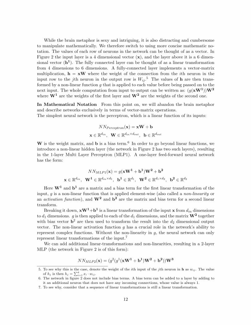
While the brain metaphor is sexy and intriguing, it is also distracting and cumbersometo manipulate mathematically. We therefore switch to using more concise mathematic no-tation. The values of each row of neurons in the network can be thought of as a vector. InFigure 2 the input layer is a 4 dimensional vector (x), and the layer above it is a 6 dimen-sional vector (h1). The fully connected layer can be thought of as a linear transformationfrom 4 dimensions to 6 dimensions. A fully-connected layer implements a vector-matrixmultiplication, h = xW where the weight of the connection from the ith neuron in theinput row to the jth neuron in the output row is Wij .

5 The values of h are then trans-formed by a non-linear function g that is applied to each value before being passed on to thenext input. The whole computation from input to output can be written as: (g(xW1))W2

where W1 are the weights of the first layer and W2 are the weights of the second one.

In Mathematical Notation From this point on, we will abandon the brain metaphorand describe networks exclusively in terms of vector-matrix operations.The simplest neural network is the perceptron, which is a linear function of its inputs:

NNPerceptron(x) = xW + b

x ∈ Rdin , W ∈ Rdin×dout , b ∈ Rdout

W is the weight matrix, and b is a bias term.6 In order to go beyond linear functions, weintroduce a non-linear hidden layer (the network in Figure 2 has two such layers), resultingin the 1-layer Multi Layer Perceptron (MLP1). A one-layer feed-forward neural networkhas the form:

NNMLP1(x) = g(xW1 + b1)W2 + b2

x ∈ Rdin , W1 ∈ Rdin×d1 , b1 ∈ Rd1 , W2 ∈ Rd1×d2 , b2 ∈ Rd2

Here W1 and b1 are a matrix and a bias term for the first linear transformation of theinput, g is a non-linear function that is applied element-wise (also called a non-linearity oran activation function), and W2 and b2 are the matrix and bias term for a second lineartransform.

Breaking it down, xW1+b1 is a linear transformation of the input x from din dimensionsto d1 dimensions. g is then applied to each of the d1 dimensions, and the matrix W2 togetherwith bias vector b2 are then used to transform the result into the d2 dimensional outputvector. The non-linear activation function g has a crucial role in the network’s ability torepresent complex functions. Without the non-linearity in g, the neural network can onlyrepresent linear transformations of the input.7

We can add additional linear-transformations and non-linearities, resulting in a 2-layerMLP (the network in Figure 2 is of this form):

NNMLP2(x) = (g2(g1(xW1 + b1)W2 + b2))W3

5. To see why this is the case, denote the weight of the ith input of the jth neuron in h as wij . The valueof hj is then hj =

∑4i=1 xi · wij .

6. The network in figure 2 does not include bias terms. A bias term can be added to a layer by adding toit an additional neuron that does not have any incoming connections, whose value is always 1.

7. To see why, consider that a sequence of linear transformations is still a linear transformation.

12

It is perhaps clearer to write deeper networks like this using intermediary variables:

NNMLP2(x) =y

h1 =g1(xW1 + b1)

h2 =g2(h1W2 + b2)

y =h2W3

The vector resulting from each linear transform is referred to as a layer. The outer-mostlinear transform results in the output layer and the other linear transforms result in hiddenlayers. Each hidden layer is followed by a non-linear activation. In some cases, such as inthe last layer of our example, the bias vectors are forced to 0 (“dropped”).

Layers resulting from linear transformations are often referred to as fully connected, oraffine. Other types of architectures exist. In particular, image recognition problems benefitfrom convolutional and pooling layers. Such layers have uses also in language processing,and will be discussed in Section 9. Networks with more than one hidden layer are said tobe deep networks, hence the name deep learning.

When describing a neural network, one should specify the dimensions of the layers andthe input. A layer will expect a din dimensional vector as its input, and transform it into adout dimensional vector. The dimensionality of the layer is taken to be the dimensionalityof its output. For a fully connected layer l(x) = xW + b with input dimensionality din andoutput dimensionality dout, the dimensions of x is 1 × din, of W is din × dout and of b is1× dout.

The output of the network is a dout dimensional vector. In case dout = 1, the network’soutput is a scalar. Such networks can be used for regression (or scoring) by consideringthe value of the output, or for binary classification by consulting the sign of the output.Networks with dout = k > 1 can be used for k-class classification, by associating eachdimension with a class, and looking for the dimension with maximal value. Similarly, ifthe output vector entries are positive and sum to one, the output can be interpreted asa distribution over class assignments (such output normalization is typically achieved byapplying a softmax transformation on the output layer, see Section 4.3).

The matrices and the bias terms that define the linear transformations are the parame-ters of the network. It is common to refer to the collection of all parameters as θ. Togetherwith the input, the parameters determine the network’s output. The training algorithm isresponsible for setting their values such that the network’s predictions are correct. Trainingis discussed in Section 6.

4.1 Representation Power

In terms of representation power, it was shown by (Hornik, Stinchcombe, & White, 1989;Cybenko, 1989) that MLP1 is a universal approximator – it can approximate with anydesired non-zero amount of error a family of functions8 that include all continuous functions

8. Specifically, a feed-forward network with linear output layer and at least one hidden layer with a “squash-ing” activation function can approximate any Borel measurable function from one finite dimensional spaceto another.

13

on a closed and bounded subset of Rn, and any function mapping from any finite dimensionaldiscrete space to another. This may suggest there is no reason to go beyond MLP1 to morecomplex architectures. However, the theoretical result does not state how large the hiddenlayer should be, nor does it say anything about the learnability of the neural network (itstates that a representation exists, but does not say how easy or hard it is to set theparameters based on training data and a specific learning algorithm). It also does notguarantee that a training algorithm will find the correct function generating our trainingdata. Since in practice we train neural networks on relatively small amounts of data, usinga combination of the backpropagation algorithm and variants of stochastic gradient descent,and use hidden layers of relatively modest sizes (up to several thousands), there is benefitto be had in trying out more complex architectures than MLP1. In many cases, however,MLP1 does indeed provide very strong results. For further discussion on the representationpower of feed-forward neural networks, see (Bengio et al., 2015, Section 6.5).

4.2 Common Non-linearities

The non-linearity g can take many forms. There is currently no good theory as to whichnon-linearity to apply in which conditions, and choosing the correct non-linearity for agiven task is for the most part an empirical question. I will now go over the common non-linearities from the literature: the sigmoid, tanh, hard tanh and the rectified linear unit(ReLU). Some NLP researchers also experimented with other forms of non-linearities suchas cube and tanh-cube.

Sigmoid The sigmoid activation function σ(x) = 1/(1 + e−x) is an S-shaped function,transforming each value x into the range [0, 1].

Hyperbolic tangent (tanh) The hyperbolic tangent tanh(x) = e2x−1e2x+1

activation func-tion is an S-shaped function, transforming the values x into the range [−1, 1].

Hard tanh The hard-tanh activation function is an approximation of the tanh functionwhich is faster to compute and take derivatives of:

hardtanh(x) =

−1 x < −1

1 x > 1

x otherwise

Rectifier (ReLU) The Rectifier activation function (Glorot, Bordes, & Bengio, 2011),also known as the rectified linear unit is a very simple activation function that is easy towork with and was shown many times to produce excellent results.9 The ReLU unit clipseach value x < 0 at 0. Despite its simplicity, it performs well for many tasks, especiallywhen combined with the dropout regularization technique (see Section 6.4).

9. The technical advantages of the ReLU over the sigmoid and tanh activation functions is that it does notinvolve expensive-to-compute functions, and more importantly that it does not saturate. The sigmoidand tanh activation are capped at 1, and the gradients at this region of the functions are near zero,driving the entire gradient near zero. The ReLU activation does not have this problem, making itespecially suitable for networks with multiple layers, which are susceptible to the vanishing gradientsproblem when trained with the saturating units.

14

ReLU(x) = max(0, x) =

{0 x < 0

x otherwise

As a rule of thumb, ReLU units work better than tanh, and tanh works better thansigmoid.10

4.3 Output Transformations

In many cases, the output layer vector is also transformed. A common transformation isthe softmax :

x =x1, . . . , xk

softmax(xi) =exi∑kj=1 e

xj

The result is a vector of non-negative real numbers that sum to one, making it a discreteprobability distribution over k possible outcomes.

The softmax output transformation is used when we are interested in modeling a prob-ability distribution over the possible output classes. To be effective, it should be used inconjunction with a probabilistic training objective such as cross-entropy (see Section 4.5below).

When the softmax transformation is applied to the output of a network without a hiddenlayer, the result is the well known multinomial logistic regression model, also known as amaximum-entropy classifier.

4.4 Embedding Layers

Up until now, the discussion ignored the source of x, treating it as an arbitrary vector.In an NLP application, x is usually composed of various embeddings vectors. We can beexplicit about the source of x, and include it in the network’s definition. We introduce c(·),a function from core features to an input vector.

It is common for c to extract the embedding vector associated with each feature, andconcatenate them:

10. In addition to these activation functions, recent works from the NLP community experiment with andreported success with other forms of non-linearities. The Cube activation function, g(x) = (x)3, wassuggested by (Chen & Manning, 2014), who found it to be more effective than other non-linearities ina feed-forward network that was used to predict the actions in a greedy transition-based dependencyparser. The tanh cube activation function g(x) = tanh((x)3 + x) was proposed by (Pei et al., 2015),who found it to be more effective than other non-linearities in a feed-forward network that was used asa component in a structured-prediction graph-based dependency parser.

The cube and tanh-cube activation functions are motivated by the desire to better capture interac-tions between different features. While these activation functions are reported to improve performancein certain situations, their general applicability is still to be determined.

15

x = c(f1, f2, f3) =[v(f1); v(f2); v(f3)]

NNMLP1(x) =NNMLP1(c(f1, f2, f3))

=NNMLP1([v(f1); v(f2); v(f3)])

=(g([v(f1); v(f2); v(f3)]W1 + b1))W2 + b2

Another common choice is for c to sum the embedding vectors (this assumes the em-bedding vectors all share the same dimensionality):

x = c(f1, f2, f3) =v(f1) + v(f2) + v(f3)

NNMLP1(x) =NNMLP1(c(f1, f2, f3))

=NNMLP1(v(f1) + v(f2) + v(f3))

=(g((v(f1) + v(f2) + v(f3))W1 + b1))W2 + b2

The form of c is an essential part of the network’s design. In many papers, it is commonto refer to c as part of the network, and likewise treat the word embeddings v(fi) as resultingfrom an “embedding layer” or “lookup layer”. Consider a vocabulary of |V | words, eachembedded as a d dimensional vector. The collection of vectors can then be thought of as a|V | × d embedding matrix E in which each row corresponds to an embedded feature. Letfi be a |V |-dimensional vector, which is all zeros except from one index, corresponding tothe value of the ith feature, in which the value is 1 (this is called a one-hot vector). Themultiplication fiE will then “select” the corresponding row of E. Thus, v(fi) can be definedin terms of E and fi:

v(fi) = fiE

And similarly:

CBOW (f1, ..., fk) =

k∑i=1

(fiE) = (

k∑i=1

fi)E

The input to the network is then considered to be a collection of one-hot vectors. Whilethis is elegant and well defined mathematically, an efficient implementation typically involvesa hash-based data structure mapping features to their corresponding embedding vectors,without going through the one-hot representation.

In this tutorial, we take c to be separate from the network architecture: the network’sinputs are always dense real-valued input vectors, and c is applied before the input is passedthe network, similar to a “feature function” in the familiar linear-models terminology. How-ever, when training a network, the input vector x does remember how it was constructed,and can propagate error gradients back to its component embedding vectors, as appropriate.

A note on notation When describing network layers that get concatenated vectors x,y and z as input, some authors use explicit concatenation ([x; y; z]W + b) while others usean affine transformation (xU + yV + zW + b). If the weight matrices U, V, W in theaffine transformation are different than one another, the two notations are equivalent.

16

A note on sparse vs. dense features Consider a network which uses a “traditional”sparse representation for its input vectors, and no embedding layer. Assuming the set of allavailable features is V and we have k “on” features f1, . . . , fk, fi ∈ V , the network’s inputis:

x =

k∑i=1

fi x ∈ N|V |+

and so the first layer (ignoring the non-linear activation) is:

xW + b = (k∑i=1

fi)W

W ∈ R|V |×d, b ∈ Rd

This layer selects rows of W corresponding to the input features in x and sums them,then adding a bias term. This is very similar to an embedding layer that produces a CBOWrepresentation over the features, where the matrix W acts as the embedding matrix. Themain difference is the introduction of the bias vector b, and the fact that the embeddinglayer typically does not undergo a non-linear activation but rather passed on directly to thefirst layer. Another difference is that this scenario forces each feature to receive a separatevector (row in W) while the embedding layer provides more flexibility, allowing for examplefor the features “next word is dog” and “previous word is dog” to share the same vector.However, these differences are small and subtle. When it comes to multi-layer feed-forwardnetworks, the difference between dense and sparse inputs is smaller than it may seem atfirst sight.

4.5 Loss Functions

When training a neural network (more on training in Section 6 below), much like whentraining a linear classifier, one defines a loss function L(y,y), stating the loss of predictingy when the true output is y. The training objective is then to minimize the loss across thedifferent training examples. The loss L(y,y) assigns a numerical score (a scalar) for thenetwork’s output y given the true expected output y.11 The loss is always positive, andshould be zero only for cases where the network’s output is correct.

The parameters of the network (the matrices Wi, the biases bi and commonly the em-beddings E) are then set in order to minimize the loss L over the training examples (usually,it is the sum of the losses over the different training examples that is being minimized).

The loss can be an arbitrary function mapping two vectors to a scalar. For practicalpurposes of optimization, we restrict ourselves to functions for which we can easily computegradients (or sub-gradients). In most cases, it is sufficient and advisable to rely on a commonloss function rather than defining your own. For a detailed discussion on loss functions forneural networks see (LeCun, Chopra, Hadsell, Ranzato, & Huang, 2006; LeCun & Huang,2005; Bengio et al., 2015). We now discuss some loss functions that are commonly used inneural networks for NLP.

11. In our notation, both the model’s output and the expected output are vectors, while in many cases it ismore natural to think of the expected output as a scalar (class assignment). In such cases, y is simplythe corresponding one-hot vector.

17

Hinge (binary) For binary classification problems, the network’s output is a single scalary and the intended output y is in {+1,−1}. The classification rule is sign(y), and aclassification is considered correct if y · y > 0, meaning that y and y share the same sign.The hinge loss, also known as margin loss or SVM loss, is defined as:

Lhinge(binary)(y, y) = max(0, 1− y · y)

The loss is 0 when y and y share the same sign and |y| ≥ 1. Otherwise, the loss is linear.In other words, the binary hinge loss attempts to achieve a correct classification, with amargin of at least 1.

Hinge (multiclass) The hinge loss was extended to the multiclass setting by Crammerand Singer (2002). Let y = y1, . . . , yn be the network’s output vector, and y be the one-hotvector for the correct output class.

The classification rule is defined as selecting the class with the highest score:

prediction = arg maxiyi

,Denote by t = arg maxi yi the correct class, and by k = arg maxi 6=t yi the highest scoring

class such that k 6= t. The multiclass hinge loss is defined as:

Lhinge(multiclass)(y,y) = max(0, 1− (yt − yk))

The multiclass hinge loss attempts to score the correct class above all other classes with amargin of at least 1.

Both the binary and multiclass hinge losses are intended to be used with a linear outputlayer. The hinge losses are useful whenever we require a hard decision rule, and do notattempt to model class membership probability.

Log loss The log loss is a common variation of the hinge loss, which can be seen as a“soft” version of the hinge loss with an infinite margin (LeCun et al., 2006).

Llog(y,y) = log(1 + exp(−(yt − yk))

Categorical cross-entropy loss The categorical cross-entropy loss (also referred to asnegative log likelihood) is used when a probabilistic interpretation of the scores is desired.

Let y = y1, . . . , yn be a vector representing the true multinomial distribution over thelabels 1, . . . , n, and let y = y1, . . . , yn be the network’s output, which was transformed by thesoftmax activation function, and represent the class membership conditional distributionyi = P (y = i|x). The categorical cross entropy loss measures the dissimilarity betweenthe true label distribution y and the predicted label distribution y, and is defined as crossentropy:

Lcross−entropy(y,y) = −∑i

yi log(yi)

18

For hard classification problems in which each training example has a single correctclass assignment, y is a one-hot vector representing the true class. In such cases, the crossentropy can be simplified to:

Lcross−entropy(hard classification)(y,y) = − log(yt)

where t is the correct class assignment. This attempts to set the probability mass assignedto the correct class t to 1. Because the scores y have been transformed using the softmaxfunction and represent a conditional distribution, increasing the mass assigned to the correctclass means decreasing the mass assigned to all the other classes.

The cross-entropy loss is very common in the neural networks literature, and produces amulti-class classifier which does not only predict the one-best class label but also predicts adistribution over the possible labels. When using the cross-entropy loss, it is assumed thatthe network’s output is transformed using the softmax transformation.

Ranking losses In some settings, we are not given supervision in term of labels, butrather as pairs of correct and incorrect items x and x′, and our goal is to score correctitems above incorrect ones. Such training situations arise when we have only positiveexamples, and generate negative examples by corrupting a positive example. A useful lossin such scenarios is the margin-based ranking loss, defined for a pair of correct and incorrectexamples:

Lranking(margin)(x,x′) = max(0, 1− (NN(x)−NN(x′)))

where NN(x) is the score assigned by the network for input vector x. The objective is toscore (rank) correct inputs over incorrect ones with a margin of at least 1.

A common variation is to use the log version of the ranking loss:

Lranking(log)(x,x′) = log(1 + exp(−(NN(x)−NN(x′))))

Examples using the ranking hinge loss in language tasks include training with the aux-iliary tasks used for deriving pre-trained word embeddings (see section 5), in which we aregiven a correct word sequence and a corrupted word sequence, and our goal is to scorethe correct sequence above the corrupt one (Collobert & Weston, 2008). Similarly, Vande Cruys (2014) used the ranking loss in a selectional-preferences task, in which the net-work was trained to rank correct verb-object pairs above incorrect, automatically derivedones, and (Weston, Bordes, Yakhnenko, & Usunier, 2013) trained a model to score correct(head,relation,trail) triplets above corrupted ones in an information-extraction setting. Anexample of using the ranking log loss can be found in (Gao et al., 2014). A variation of theranking log loss allowing for a different margin for the negative and positive class is givenin (dos Santos et al., 2015).

19

5. Word Embeddings

A main component of the neural-network approach is the use of embeddings – representingeach feature as a vector in a low dimensional space. But where do the vectors come from?This section will survey the common approaches.

5.1 Random Initialization

When enough supervised training data is available, one can just treat the feature embeddingsthe same as the other model parameters: initialize the embedding vectors to random values,and let the network-training procedure tune them into “good” vectors.

Some care has to be taken in the way the random initialization is performed. The methodused by the effective word2vec implementation (Mikolov et al., 2013; Mikolov, Sutskever,Chen, Corrado, & Dean, 2013) is to initialize the word vectors to uniformly sampled randomnumbers in the range [− 1

2d ,12d ] where d is the number of dimensions. Another option is to

use xavier initialization (see Section 6.3) and initialize with uniformly sampled values from[−√

6√d,√

6√d

].

In practice, one will often use the random initialization approach to initialize the em-bedding vectors of commonly occurring features, such as part-of-speech tags or individualletters, while using some form of supervised or unsupervised pre-training to initialize thepotentially rare features, such as features for individual words. The pre-trained vectors canthen either be treated as fixed during the network training process, or, more commonly,treated like the randomly-initialized vectors and further tuned to the task at hand.

5.2 Supervised Task-specific Pre-training

If we are interested in task A, for which we only have a limited amount of labeled data (forexample, syntactic parsing), but there is an auxiliary task B (say, part-of-speech tagging)for which we have much more labeled data, we may want to pre-train our word vectors sothat they perform well as predictors for task B, and then use the trained vectors for trainingtask A. In this way, we can utilize the larger amounts of labeled data we have for task B.When training task A we can either treat the pre-trained vectors as fixed, or tune themfurther for task A. Another option is to train jointly for both objectives, see Section 7 formore details.

5.3 Unsupervised Pre-training

The common case is that we do not have an auxiliary task with large enough amounts ofannotated data (or maybe we want to help bootstrap the auxiliary task training with bettervectors). In such cases, we resort to “unsupervised” methods, which can be trained on hugeamounts of unannotated text.

The techniques for training the word vectors are essentially those of supervised learning,but instead of supervision for the task that we care about, we instead create practically

20

unlimited number of supervised training instances from raw text, hoping that the tasksthat we created will match (or be close enough to) the final task we care about.12

The key idea behind the unsupervised approaches is that one would like the embeddingvectors of “similar” words to have similar vectors. While word similarity is hard to defineand is usually very task-dependent, the current approaches derive from the distributionalhypothesis (Harris, 1954), stating that words are similar if they appear in similar contexts.The different methods all create supervised training instances in which the goal is to eitherpredict the word from its context, or predict the context from the word.

An important benefit of training word embeddings on large amounts of unannotateddata is that it provides vector representations for words that do not appear in the super-vised training set. Ideally, the representations for these words will be similar to those ofrelated words that do appear in the training set, allowing the model to generalize better onunseen events. It is thus desired that the similarity between word vectors learned by the un-supervised algorithm captures the same aspects of similarity that are useful for performingthe intended task of the network.

Common unsupervised word-embedding algorithms include word2vec 13 (Mikolov et al.,2013, 2013), GloVe (Pennington, Socher, & Manning, 2014) and the Collobert and Weston(2008, 2011) embeddings algorithm. These models are inspired by neural networks andare based on stochastic gradient training. However, they are deeply connected to anotherfamily of algorithms which evolved in the NLP and IR communities, and that are based onmatrix factorization (see (Levy & Goldberg, 2014b; Levy et al., 2015) for a discussion).

Arguably, the choice of auxiliary problem (what is being predicted, based on what kindof context) affects the resulting vectors much more than the learning method that is beingused to train them. We thus focus on the different choices of auxiliary problems that areavailable, and only skim over the details of the training methods. Several software packagesfor deriving word vectors are available, including word2vec14 and Gensim15 implementingthe word2vec models with word-windows based contexts, word2vecf16 which is a modifiedversion of word2vec allowing the use of arbitrary contexts, and GloVe17 implementing theGloVe model. Many pre-trained word vectors are also available for download on the web.

While beyond the scope of this tutorial, it is worth noting that the word embeddingsderived by unsupervised training algorithms have a wide range of applications in NLPbeyond using them for initializing the word-embeddings layer of a neural-network model.

5.4 Training Objectives

Given a word w and its context c, different algorithms formulate different auxiliary tasks.In all cases, each word is represented as a d-dimensional vector which is initialized to arandom value. Training the model to perform the auxiliary tasks well will result in good

12. The interpretation of creating auxiliary problems from raw text is inspired by Ando and Zhang (Ando& Zhang, 2005a, 2005b).

13. While often treated as a single algorithm, word2vec is actually a software package including varioustraining objectives, optimization methods and other hyperparameters. See (Rong, 2014; Levy, Goldberg,& Dagan, 2015) for a discussion.

14. https://code.google.com/p/word2vec/15. https://radimrehurek.com/gensim/16. https://bitbucket.org/yoavgo/word2vecf17. http://nlp.stanford.edu/projects/glove/

21

word embeddings for relating the words to the contexts, which in turn will result in theembedding vectors for similar words to be similar to each other.

Language-modeling inspired approaches such as those taken by (Mikolov et al., 2013;Mnih & Kavukcuoglu, 2013) as well as GloVe (Pennington et al., 2014) use auxiliary tasksin which the goal is to predict the word given its context. This is posed in a probabilisticsetup, trying to model the conditional probability P (w|c).

Other approaches reduce the problem to that of binary classification. In addition tothe set D of observed word-context pairs, a set D is created from random words andcontext pairings. The binary classification problem is then: does the given (w, c) paircome from D or not? The approaches differ in how the set D is constructed, what isthe structure of the classifier, and what is the objective being optimized. Collobert andWeston (2008, 2011) take a margin-based binary ranking approach, training a feed-forwardneural network to score correct (w, c) pairs over incorrect ones. Mikolov et al (2013, 2014)take instead a probabilistic version, training a log-bilinear model to predict the probabilityP ((w, c) ∈ D|w, c) that the pair come from the corpus rather than the random sample.

5.5 The Choice of Contexts

In most cases, the contexts of a word are taken to be other words that appear in itssurrounding, either in a short window around it, or within the same sentence, paragraphor document. In some cases the text is automatically parsed by a syntactic parser, andthe contexts are derived from the syntactic neighbourhood induced by the automatic parsetrees. Sometimes, the definitions of words and context change to include also parts of words,such as prefixes or suffixes.

Neural word embeddings originated from the world of language modeling, in which anetwork is trained to predict the next word based on a sequence of preceding words (Bengioet al., 2003). There, the text is used to create auxiliary tasks in which the aim is to predicta word based on a context the k previous words. While training for the language modelingauxiliary prediction problems indeed produce useful embeddings, this approach is needlesslyrestricted by the constraints of the language modeling task, in which one is allowed to lookonly at the previous words. If we do not care about language modeling but only about theresulting embeddings, we may do better by ignoring this constraint and taking the contextto be a symmetric window around the focus word.

5.5.1 Window Approach

The most common approach is a sliding window approach, in which auxiliary tasks arecreated by looking at a sequence of 2k+ 1 words. The middle word is callled the focus wordand the k words to each side are the contexts. Then, either a single task is created in whichthe goal is to predict the focus word based on all of the context words (represented eitherusing CBOW (Mikolov et al., 2013) or vector concatenation (Collobert & Weston, 2008)),or 2k distinct tasks are created, each pairing the focus word with a different context word.The 2k tasks approach, popularized by (Mikolov et al., 2013) is referred to as a skip-grammodel. Skip-gram based approaches are shown to be robust and efficient to train (Mikolovet al., 2013; Pennington et al., 2014), and often produce state of the art results.

22

Effect of Window Size The size of the sliding window has a strong effect on the re-sulting vector similarities. Larger windows tend to produce more topical similarities (i.e.“dog”, “bark” and “leash” will be grouped together, as well as “walked”, “run” and “walk-ing”), while smaller windows tend to produce more functional and syntactic similarities (i.e.“Poodle”, “Pitbull”, “Rottweiler”, or “walking”,“running”,“approaching”).

Positional Windows When using the CBOW or skip-gram context representations, allthe different context words within the window are treated equally. There is no distinctionbetween context words that are close to the focus words and those that are farther fromit, and likewise there is no distinction between context words that appear before the focuswords to context words that appear after it. Such information can easily be factored in byusing positional contexts: indicating for each context word also its relative position to thefocus words (i.e. instead of the context word being “the” it becomes “the:+2”, indicatingthe word appears two positions to the right of the focus word). The use of positional contexttogether with smaller windows tend to produce similarities that are more syntactic, witha strong tendency of grouping together words that share a part of speech, as well as beingfunctionally similar in terms of their semantics. Positional vectors were shown by (Ling,Dyer, Black, & Trancoso, 2015a) to be more effective than window-based vectors when usedto initialize networks for part-of-speech tagging and syntactic dependency parsing.

Variants Many variants on the window approach are possible. One may lemmatize wordsbefore learning, apply text normalization, filter too short or too long sentences, or removecapitalization (see, e.g., the pre-processing steps described in (dos Santos & Gatti, 2014).One may sub-sample part of the corpus, skipping with some probability the creation of tasksfrom windows that have too common or too rare focus words. The window size may bedynamic, using a different window size at each turn. One may weigh the different positionsin the window differently, focusing more on trying to predict correctly close word-contextpairs than further away ones. Each of these choices will effect the resulting vectors. Someof these hyperparameters (and others) are discussed in (Levy et al., 2015).

5.5.2 Sentences, Paragraphs or Documents

Using a skip-grams (or CBOW) approach, one can consider the contexts of a word to be allthe other words that appear with it in the same sentence, paragraph or document. This isequivalent to using very large window sizes, and is expected to result in word vectors thatcapture topical similarity (words from the same topic, i.e. words that one would expect toappear in the same document, are likely to receive similar vectors).

5.5.3 Syntactic Window

Some work replace the linear context within a sentence with a syntactic one (Levy &Goldberg, 2014a; Bansal, Gimpel, & Livescu, 2014). The text is automatically parsedusing a dependency parser, and the context of a word is taken to be the words that arein its proximity in the parse tree, together with the syntactic relation by which they areconnected. Such approaches produce highly functional similarities, grouping together wordsthan can fill the same role in a sentence (e.g. colors, names of schools, verbs of movement).

23

The grouping is also syntactic, grouping together words that share an inflection (Levy &Goldberg, 2014a).

5.5.4 Multilingual

Another option is using multilingual, translation based contexts (Hermann & Blunsom,2014; Faruqui & Dyer, 2014). For example, given a large amount of sentence-aligned paralleltext, one can run a bilingual alignment model such as the IBM model 1 or model 2 (i.e.using the GIZA++ software), and then use the produced alignments to derive word contexts.Here, the context of a word instance are the foreign language words that are aligned to it.Such alignments tend to result in synonym words receiving similar vectors. Some authorswork instead on the sentence alignment level, without relying on word alignments. Anappealing method is to mix a monolingual window-based approach with a multilingualapproach, creating both kinds of auxiliary tasks. This is likely to produce vectors that aresimilar to the window-based approach, but reducing the somewhat undesired effect of thewindow-based approach in which antonyms (e.g. hot and cold, high and low) tend to receivesimilar vectors (Faruqui & Dyer, 2014).

5.5.5 Character-based and Sub-word Representations

An interesting line of work attempts to derive the vector representation of a word from thecharacters that compose it. Such approaches are likely to be particularly useful for taskswhich are syntactic in nature, as the character patterns within words are strongly relatedto their syntactic function. These approaches also have the benefit of producing very smallmodel sizes (only one vector for each character in the alphabet together with a handful ofsmall matrices needs to be stored), and being able to provide an embedding vector for everyword that may be encountered. dos Santos and Gatti (2014) and dos Santos and Zadrozny(2014) model the embedding of a word using a convolutional network (see Section 9) overthe characters. Ling et al (2015b) model the embedding of a word using the concatenationof the final states of two RNN (LSTM) encoders (Section 10), one reading the charactersfrom left to right, and the other from right to left. Both produce very strong results forpart-of-speech tagging. The work of Ballesteros et al (2015) show that the two-LSTMsencoding of (Ling et al., 2015b) is beneficial also for representing words in dependencyparsing of morphologically rich languages.

Deriving representations of words from the representations of their characters is moti-vated by the unknown words problem – what do you do when you encounter a word forwhich you do not have an embedding vector? Working on the level of characters alleviatesthis problem to a large extent, as the vocabulary of possible characters is much smallerthan the vocabulary of possible words. However, working on the character level is verychallenging, as the relationship between form (characters) and function (syntax, semantics)in language is quite loose. Restricting oneself to stay on the character level may be anunnecessarily hard constraint. Some researchers propose a middle-ground, in which a wordis represented as a combination of a vector for the word itself with vectors of sub-wordunits that comprise it. The sub-word embeddings then help in sharing information betweendifferent words with similar forms, as well as allowing back-off to the subword level whenthe word is not observed. At the same time, the models are not forced to rely solely on

24

form when enough observations of the word are available. Botha and Blunsom (2014) sug-gest to model the embedding vector of a word as a sum of the word-specific vector if suchvector is available, with vectors for the different morphological components that compriseit (the components are derived using Morfessor (Creutz & Lagus, 2007), an unsupervisedmorphological segmentation method). Gao et al (Gao et al., 2014) suggest using as corefeatures not only the word form itself but also a unique feature (hence a unique embeddingvector) for each of the letter-trigrams in the word.

25

6. Neural Network Training

Neural network training is done by trying to minimize a loss function over a training set,using a gradient-based method. Roughly speaking, all training methods work by repeatedlycomputing an estimate of the error over the dataset, computing the gradient with respectto the error, and then moving the parameters in the direction of the gradient. Models differin how the error estimate is computed, and how “moving in the direction of the gradient”is defined. We describe the basic algorithm, stochastic gradient descent (SGD), and thenbriefly mention the other approaches with pointers for further reading. Gradient calculationis central to the approach. Gradients can be efficiently and automatically computed usingreverse mode differentiation on a computation graph – a general algorithmic framework forautomatically computing the gradient of any network and loss function.

6.1 Stochastic Gradient Training

The common approach for training neural networks is using the stochastic gradient descent(SGD) algorithm (Bottou, 2012; LeCun, Bottou, Orr, & Muller, 1998a) or a variant of it.SGD is a general optimization algorithm. It receives a function f parameterized by θ, aloss function, and desired input and output pairs. It then attempts to set the parameters θsuch that the loss of f with respect to the training examples is small. The algorithm worksas follows:

Algorithm 1 Online Stochastic Gradient Descent Training

1: Input: Function f(x; θ) parameterized with parameters θ.2: Input: Training set of inputs x1, . . . ,xn and outputs y1, . . . ,yn.3: Input: Loss function L.4: while stopping criteria not met do5: Sample a training example xi,yi

6: Compute the loss L(f(xi; θ),yi)7: g← gradients of L(f(xi; θ),yi) w.r.t θ8: θ ← θ + ηkg

9: return θ

The goal of the algorithm is to set the parameters θ so as to minimize the total loss∑ni=1 L(f(xi; θ),yi) over the training set. It works by repeatedly sampling a training exam-

ple and computing the gradient of the error on the example with respect to the parametersθ (line 7) – the input and expected output are assumed to be fixed, and the loss is treatedas a function of the parameters θ. The parameters θ are then updated in the direction ofthe gradient, scaled by a learning rate ηk (line 8). For further discussion on setting thelearning rate, see Section 6.3.

Note that the error calculated in line 6 is based on a single training example, and is thusjust a rough estimate of the corpus-wide loss that we are aiming to minimize. The noise inthe loss computation may result in inaccurate gradients. A common way of reducing thisnoise is to estimate the error and the gradients based on a sample of m examples. Thisgives rise to the minibatch SGD algorithm:

26

Algorithm 2 Minibatch Stochastic Gradient Descent Training

1: Input: Function f(x; θ) parameterized with parameters θ.2: Input: Training set of inputs x1, . . . ,xn and outputs y1, . . . ,yn.3: Input: Loss function L.4: while stopping criteria not met do5: Sample a minibatch of m examples {(x1,y1), . . . , (xm,ym)}6: g← 07: for i = 1 to m do8: Compute the loss L(f(xi; θ),yi)9: g← g + gradients of 1

mL(f(xi; θ),yi) w.r.t θ

10: θ ← θ + ηkg

11: return θ

In lines 6 – 9 the algorithm estimates the gradient of the corpus loss based on theminibatch. After the loop, g contains the gradient estimate, and the parameters θ areupdated toward g. The minibatch size can vary in size from m = 1 to m = n. Highervalues provide better estimates of the corpus-wide gradients, while smaller values allowmore updates and in turn faster convergence. Besides the improved accuracy of the gradientsestimation, the minibatch algorithm provides opportunities for improved training efficiency.For modest sizes of m, some computing architectures (i.e. GPUs) allow an efficient parallelimplementation of the computation in lines 6–9. With a small enough learning rate, SGD isguaranteed to converge to a global optimum if the function is convex. However, it can alsobe used to optimize non-convex functions such as neural-network. While there are no longerguarantees of finding a global optimum, the algorithm proved to be robust and performswell in practice.

When training a neural network, the parameterized function f is the neural network,and the parameters θ are the layer-transfer matrices, bias terms, embedding matrices andso on. The gradient computation is a key step in the SGD algorithm, as well as in allother neural network training algorithms. The question is, then, how to compute thegradients of the network’s error with respect to the parameters. Fortunately, there is an easysolution in the form of the backpropagation algorithm (Rumelhart, Hinton, & Williams, 1986;Lecun, Bottou, Bengio, & Haffner, 1998b). The backpropagation algorithm is a fancy namefor methodologically computing the derivatives of a complex expression using the chain-rule, while caching intermediary results. More generally, the backpropagation algorithmis a special case of the reverse-mode automatic differentiation algorithm (Neidinger, 2010,Section 7), (Baydin, Pearlmutter, Radul, & Siskind, 2015; Bengio, 2012).The followingsection describes reverse mode automatic differentiation in the context of the computationgraph abstraction.

Beyond SGD While the SGD algorithm can and often does produce good results, moreadvanced algorithms are also available. The SGD+Momentum (Polyak, 1964) and NesterovMomentum (Sutskever, Martens, Dahl, & Hinton, 2013) algorithms are variants of SGD inwhich previous gradients are accumulated and affect the current update. Adaptive learningrate algorithms including AdaGrad (Duchi, Hazan, & Singer, 2011), AdaDelta (Zeiler, 2012),

27

RMSProp (Tieleman & Hinton, 2012) and Adam (Kingma & Ba, 2014) are designed toselect the learning rate for each minibatch, sometimes on a per-coordinate basis, potentiallyalleviating the need of fiddling with learning rate scheduling. For details of these algorithms,see the original papers or (Bengio et al., 2015, Sections 8.3, 8.4). As many neural-networksoftware frameworks provide implementations of these algorithms, it is easy and sometimesworthwhile to try out different variants.

6.2 The Computation Graph Abstraction

While one can compute the gradients of the various parameters of a network by hand andimplement them in code, this procedure is cumbersome and error prone. For most pur-poses, it is preferable to use automatic tools for gradient computation (Bengio, 2012). Thecomputation-graph abstraction allows us to easily construct arbitrary networks, evaluatetheir predictions for given inputs (forward pass), and compute gradients for their parameterswith respect to arbitrary scalar losses (backward pass).

A computation graph is a representation of an arbitrary mathematical computation asa graph. It is a directed acyclic graph (DAG) in which nodes correspond to mathematicaloperations or (bound) variables and edges correspond to the flow of intermediary valuesbetween the nodes. The graph structure defines the order of the computation in terms ofthe dependencies between the different components. The graph is a DAG and not a tree, asthe result of one operation can be the input of several continuations. Consider for examplea graph for the computation of (a ∗ b+ 1) ∗ (a ∗ b+ 2):

a b1 2

*++

*

The computation of a∗b is shared. We restrict ourselves to the case where the computationgraph is connected.

Since a neural network is essentially a mathematical expression, it can be representedas a computation graph.

For example, Figure 3a presents the computation graph for a 1-layer MLP with a soft-max output transformation. In our notation, oval nodes represent mathematical operationsor functions, and shaded rectangle nodes represent parameters (bound variables). Networkinputs are treated as constants, and drawn without a surrounding node. Input and param-eter nodes have no incoming arcs, and output nodes have no outgoing arcs. The output ofeach node is a matrix, the dimensionality of which is indicated above the node.

This graph is incomplete: without specifying the inputs, we cannot compute an output.Figure 3b shows a complete graph for an MLP that takes three words as inputs, and predictsthe distribution over part-of-speech tags for the third word. This graph can be used forprediction, but not for training, as the output is a vector (not a scalar) and the graph doesnot take into account the correct answer or the loss term. Finally, the graph in 3c shows thecomputation graph for a specific training example, in which the inputs are the (embeddings

28

x1× 150

W1

150× 20

MUL

1× 20

ADD

1× 20

b1

1× 20

tanh

1× 20

W2

20× 17

b2

1× 17

MUL

1× 17

ADD

1× 17

softmax

1× 17

(a)

concat

1× 150

lookup

1× 50

lookup

1× 50

lookup

1× 50

“the” “black” “dog” E

|V | × 50

W1

150× 20

MUL

1× 20

ADD

1× 20

b1

1× 20

tanh

1× 20

W2

20× 17

b2

1× 17

MUL

1× 17

ADD

1× 17

softmax

1× 17

(b)

concat

1× 150

lookup

1× 50

lookup

1× 50

lookup

1× 50

“the” “black” “dog” E

|V | × 50

W1

150× 20

MUL

1× 20

ADD

1× 20

b1

1× 20

tanh

1× 20

W2

20× 17

b2

1× 17

MUL

1× 17

ADD

1× 17

softmax

1× 17

pick

1× 1

5

log

1× 1

neg

1× 1

(c)

Figure 3: Computation Graph for MLP1. (a) Graph with unbound input. (b) Graphwith concrete input. (c) Graph with concrete input, expected output, and lossnode.

of) the words “the”, “black”, “dog”, and the expected output is “NOUN” (whose index is5).

Once the graph is built, it is straightforward to run either a forward computation (com-pute the result of the computation) or a backward computation (computing the gradients),as we show below. Constructing the graphs may look daunting, but is actually very easyusing dedicated software libraries and APIs.

Forward Computation The forward pass computes the outputs of the nodes in thegraph. Since each node’s output depends only on itself and on its incoming edges, it istrivial to compute the outputs of all nodes by traversing the nodes in a topological order andcomputing the output of each node given the already computed outputs of its predecessors.

More formally, in a graph of N nodes, we associate each node with an index i accordingto their topological ordering. Let fi be the function computed by node i (e.g. multiplication.addition, . . . ). Let π(i) be the parent nodes of node i, and π−1(i) = {j | i ∈ π(j)} thechildren nodes of node i (these are the arguments of fi). Denote by v(i) the output of node

29

i, that is, the application of fi to the output values of its arguments π−1(i). For variableand input nodes, fi is a constant function and π−1(i) is empty. The Forward algorithmcomputes the values v(i) for all i ∈ [1, N ].

Algorithm 3 Computation Graph Forward Pass

1: for i = 1 to N do2: Let a1, . . . , am = π−1(i)3: v(i)← fi(v(a1), . . . , v(am))

Backward Computation (Derivatives, Backprop) The backward pass begins by des-ignating a node N with scalar (1× 1) output as a loss-node, and running forward computa-tion up to that node. The backward computation will computes the gradients with respect

to that node’s value. Denote by d(i) the quantity∂N

∂i. The backpropagation algorithm is

used to compute the values d(i) for all nodes i.The backward pass fills a table d(i) as follows:

Algorithm 4 Computation Graph Backward Pass (Backpropagation)

1: d(N)← 12: for i = N-1 to 1 do

3: d(i)←∑j∈π(i) d(j) · ∂fj

∂i

The quantity∂fj∂i

is the partial derivative of fj(π−1(j)) w.r.t the argument i ∈ π−1(j).

This value depends on the function fj and the values v(a1), . . . , v(am) (where a1, . . . , am =π−1(j)) of its arguments, which were computed in the forward pass.

Thus, in order to define a new kind of node, one need to define two methods: one forcalculating the forward value v(i) based on the nodes inputs, and the another for calculating∂fi∂x

for each x ∈ π−1(i).

For further information on automatic differentiation see (Neidinger, 2010, Section 7),(Baydin et al., 2015). For more in depth discussion of the backpropagation algorithm andcomputation graphs (also called flow graphs) see (Bengio et al., 2015, Section 6.4), (Lecunet al., 1998b; Bengio, 2012). For a popular yet technical presentation, see Chris Olah’sdescription at http://colah.github.io/posts/2015-08-Backprop/.

Software Several software packages implement the computation-graph model, includingTheano18, Chainer19, penne20 and CNN/pyCNN21. All these packages support all the es-sential components (node types) for defining a wide range of neural network architectures,covering the structures described in this tutorial and more. Graph creation is made almosttransparent by use of operator overloading. The framework defines a type for representinggraph nodes (commonly called expressions), methods for constructing nodes for inputs and

18. http://deeplearning.net/software/theano/19. http://chainer.org20. https://bitbucket.org/ndnlp/penne21. https://github.com/clab/cnn

30

parameters, and a set of functions and mathematical operations that take expressions asinput and result in more complex expressions. For example, the python code for creatingthe computation graph from Figure (3c) using the pyCNN framework is:

from pycnn import *# model initialization.model = Model()model.add_parameters("W1", (20,150))model.add_parameters("b1", 20)model.add_parameters("W2", (17,20))model.add_parameters("b2", 17)model.add_lookup_parameters("words", (100, 50))

# Building the computation graph:renew_cg() # create a new graph.# Wrap the model parameters as graph-nodes.W1 = parameter(model["W1"])b1 = parameter(model["b1"])W2 = parameter(model["W2"])b2 = parameter(model["b2"])def get_index(x): return 1# Generate the embeddings layer.vthe = lookup(model["words"], get_index("the"))vblack = lookup(model["words"], get_index("black"))vdog = lookup(model["words"], get_index("dog"))

# Connect the leaf nodes into a complete graph.x = concatenate([vthe, vblack, vdog])output = softmax(W2*(tanh(W1*x)+b1)+b2)loss = -log(pick(output, 5))

loss_value = loss.forward()loss.backward() # the gradient is computed

# and stored in the corresponding# parameters.

Most of the code involves various initializations: the first block defines model parametersthat are be shared between different computation graphs (recall that each graph correspondsto a specific training example). The second block turns the model parameters into the graph-node (Expression) types. The third block retrieves the Expressions for the embeddings of theinput words. Finally, the fourth block is where the graph is created. Note how transparentthe graph creation is – there is an almost a one-to-one correspondence between creatingthe graph and describing it mathematically. The last block shows a forward and backwardpass. The other software frameworks follow similar patterns.

Theano involves an optimizing compiler for computation graphs, which is both a blessingand a curse. On the one hand, once compiled, large graphs can be run efficiently on eitherthe CPU or a GPU, making it ideal for large graphs with a fixed structure, where only theinputs change between instances. However, the compilation step itself can be costly, and itmakes the interface a bit cumbersome to work with. In contrast, the other packages focus onbuilding large and dynamic computation graphs and executing them “on the fly” without acompilation step. While the execution speed may suffer with respect to Theano’s optimizedversion, these packages are especially convenient when working with the recurrent and

31

recursive networks described in Sections 10, 12 as well as in structured prediction settingsas described in Section 8.

Implementation Recipe Using the computation graph abstraction, the pseudo-code fora network training algorithm is given in Algorithm 5.

Algorithm 5 Neural Network Training with Computation Graph Abstraction (using mini-batches of size 1)

1: Define network parameters.2: for iteration = 1 to N do3: for Training example xi,yi in dataset do4: loss node ← build computation graph(xi, yi, parameters)5: loss node.forward()6: gradients ← loss node().backward()7: parameters ← update parameters(parameters, gradients)

8: return parameters.

Here, build computation graph is a user-defined function that builds the computationgraph for the given input, output and network structure, returning a single loss node.update parameters is an optimizer specific update rule. The recipe specifies that a newgraph is created for each training example. This accommodates cases in which the networkstructure varies between training example, such as recurrent and recursive neural networks,to be discussed in Sections 10 – 12. For networks with fixed structures, such as an MLPs, itmay be more efficient to create one base computation graph and vary only the inputs andexpected outputs between examples.

Network Composition As long as the network’s output is a vector (1 × k matrix), itis trivial to compose networks by making the output of one network the input of another,creating arbitrary networks. The computation graph abstractions makes this ability explicit:a node in the computation graph can itself be a computation graph with a designated outputnode. One can then design arbitrarily deep and complex networks, and be able to easilyevaluate and train them thanks to automatic forward and gradient computation. This makesit easy to define and train networks for structured outputs and multi-objective training, aswe discuss in Section 7, as well as complex recurrent and recursive networks, as discussedin Sections 10–12.

6.3 Optimization Issues

Once the gradient computation is taken care of, the network is trained using SGD or anothergradient-based optimization algorithm. The function being optimized is not convex, and fora long time training of neural networks was considered a “black art” which can only be doneby selected few. Indeed, many parameters affect the optimization process, and care has tobe taken to tune these parameters. While this tutorial is not intended as a comprehensiveguide to successfully training neural networks, we do list here a few of the prominent issues.For further discussion on optimization techniques and algorithms for neural networks, referto (Bengio et al., 2015, Chapter 8). For some theoretical discussion and analysis, refer

32

to (Glorot & Bengio, 2010). For various practical tips and recommendations, see (LeCunet al., 1998a; Bottou, 2012).

Initialization The non-convexity of the loss function means the optimization proceduremay get stuck in a local minimum or a saddle point, and that starting from different initialpoints (e.g. different random values for the parameters) may result in different results. Thus,it is advised to run several restarts of the training starting at different random initializations,and choosing the best one based on a development set.22 The amount of variance in theresults is different for different network formulations and datasets, and cannot be predictedin advance.

The magnitude of the random values has an important effect on the success of training.An effective scheme due to Glorot and Bengio (2010), called xavier initialization afterGlorot’s first name, suggests initializing a weight matrix W ∈ Rdin×dout as:

W ∼ U[−

√6√

din + dout,+

√6√

din + dout

]

where U [a, b] is a uniformly sampled random value in the range [a, b]. This advice workswell on many occasions, and is the preferred default initialization method by many.

Analysis by He et al (2015) suggests that when using ReLU non-linearities, the weightsshould be initialized by sampling from a zero-mean Gaussian distribution whose standard

deviation is√

2din

. This initialization was found by He et al to work better than xavier

initialization in an image classification task, especially when deep networks were involved.

Vanishing and Exploding Gradients In deep networks, it is common for the errorgradients to either vanish (become exceedingly close to 0) or explode (become exceedinglyhigh) as they propagate back through the computation graph. The problem becomes moresevere in deeper networks, and especially so in recursive and recurrent networks (Pascanu,Mikolov, & Bengio, 2012). Dealing with the vanishing gradients problem is still an openresearch question. Solutions include making the networks shallower, step-wise training (firsttrain the first layers based on some auxiliary output signal, then fix them and train the upperlayers of the complete network based on the real task signal), or specialized architecturesthat are designed to assist in gradient flow (e.g., the LSTM and GRU architectures forrecurrent networks, discussed in Section 11). Dealing with the exploding gradients hasa simple but very effective solution: clipping the gradients if their norm exceeds a giventhreshold. Let g be the gradients of all parameters in the network, and ‖g‖ be their L2

norm. Pascanu et al (2012) suggest to set: g← threshold‖g‖ g if ‖g‖ > threshold.

Saturation and Dead Neurons Layers with tanh and sigmoid activations can becomesaturated – resulting in output values for that layer that are all close to one, the upper-limit of the activation function. Saturated neurons have very small gradients, and shouldbe avoided. Layers with the ReLU activation cannot be saturated, but can “die” – most orall values are negative and thus clipped at zero for all inputs, resulting in a gradient of zerofor that layer. If your network does not train well, it is advisable to monitor the networkfor layers with many saturated or dead neurons. Saturated neurons are caused by too large

22. When debugging, and for reproducibility of results, it is advised to used a fixed random seed.

33

values entering the layer. This may be controlled for by changing the initialization, scalingthe range of the input values, or changing the learning rate. Dead neurons are caused byall weights entering the layer being negative (for example this can happen after a largegradient update). Reducing the learning rate will help in this situation. For saturatedlayers, another option is to normalize the values in the saturated layer after the activation,i.e. instead of g(h) = tanh(h) using g(h) = tanh(h)

‖tanh(h)‖ . Layer normalization is an effectivemeasure for countering saturation, but is also expensive in terms of gradient computation.

Shuffling The order in which the training examples are presented to the network is im-portant. The SGD formulation above specifies selecting a random example in each turn.In practice, most implementations go over the training example in order. It is advised toshuffle the training examples before each pass through the data.

Learning Rate Selection of the learning rate is important. Too large learning rateswill prevent the network from converging on an effective solution. Too small learningrates will take very long time to converge. As a rule of thumb, one should experimentwith a range of initial learning rates in range [0, 1], e.g. 0.001, 0.01, 0.1, 1. Monitorthe network’s loss over time, and decrease the learning rate once the network seem to bestuck in a fixed region. Learning rate scheduling decrease the rate as a function of thenumber of observed minibatches. A common schedule is dividing the initial learning rateby the iteration number. Leon Bottou (2012) recommends using a learning rate of the formηt = η0(1 + η0λt)

−1 where η0 is the initial learning rate, ηt is the learning rate to use onthe tth training example, and λ is an additional hyperparameter. He further recommendsdetermining a good value of η0 based on a small sample of the data prior to running on theentire dataset.

Minibatches Parameter updates occur either every training example (minibatches of size1) or every k training examples. Some problems benefit from training with larger minibatchsizes. In terms of the computation graph abstraction, one can create a computation graphfor each of the k training examples, and then connecting the k loss nodes under an averagingnode, whose output will be the loss of the minibatch. Large minibatched training can alsobe beneficial in terms of computation efficiency on specialized computing architectures suchas GPUs. This is beyond the scope of this tutorial.

6.4 Regularization

Neural network models have many parameters, and overfitting can easily occur. Overfittingcan be alleviated to some extent by regularization. A common regularization method isL2 regularization, placing a squared penalty on parameters with large values by addingan additive λ

2‖θ‖2 term to the objective function to be minimized, where θ is the set ofmodel parameters, ‖ · ‖2 is the squared L2 norm (sum of squares of the values), and λ is ahyperparameter controlling the amount of regularization.

A recently proposed alternative regularization method is dropout (Hinton, Srivastava,Krizhevsky, Sutskever, & Salakhutdinov, 2012). The dropout method is designed to preventthe network from learning to rely on specific weights. It works by randomly dropping (set-ting to 0) half of the neurons in the network (or in a specific layer) in each training example.Work by Wager et al (2013) establishes a strong connection between the dropout method

34

and L2 regularization. Gal and Gharamani (2015) show that a multi-layer perceptron withdropout applied at every layer can be interpreted as Bayesian model averaging.

The dropout technique is one of the key factors contributing to very strong results ofneural-network methods on image classification tasks (Krizhevsky, Sutskever, & Hinton,2012), especially when combined with ReLU activation units (Dahl, Sainath, & Hinton,2013). The dropout technique is effective also in NLP applications of neural networks.

35

7. Cascading and Multi-task Learning

The combination of online training methods with automatic gradient computations usingthe computation graph abstraction allows for an easy implementation of model cascading,parameter sharing and multi-task learning.

Model cascading is a powerful technique in which large networks are built by composingthem out of smaller component networks. For example, we may have a feed-forward networkfor predicting the part of speech of a word based on its neighbouring words and/or thecharacters that compose it. In a pipeline approach, we would use this network for predictingparts of speech, and then feed the predictions as input features to neural network that doessyntactic chunking or parsing. Instead, we could think of the hidden layers of this networkas an encoding that captures the relevant information for predicting the part of speech. Ina cascading approach, we take the hidden layers of this network and connect them (and notthe part of speech prediction themselves) as the inputs for the syntactic network. We nowhave a larger network that takes as input sequences of words and characters, and outputs asyntactic structure. The computation graph abstraction allows us to easily propagate theerror gradients from the syntactic task loss all the way back to the characters.

To combat the vanishing gradient problem of deep networks, as well as to make betteruse of available training material, the individual component network’s parameters can bebootstrapped by training them separately on a relevant task, before plugging them in tothe larger network for further tuning. For example, the part-of-speech predicting networkcan be trained to accurately predict parts-of-speech on a relatively large annotated corpus,before plugging its hidden layer into the syntactic parsing network for which less trainingdata is available. In case the training data provide direct supervision for both tasks, we canmake use of it during training by creating a network with two outputs, one for each task,computing a separate loss for each output, and then summing the losses into a single nodefrom which we backpropagate the error gradients.

Model cascading is very common when using convolutional, recursive and recurrentneural networks, where, for example, a recurrent network is used to encode a sentence intoa fixed sized vector, which is then used as the input of another network. The supervisionsignal of the recurrent network comes primarily from the upper network that consumes therecurrent network’s output as it inputs.

Multi-task learning is used when we have related prediction tasks that do not neces-sarily feed into one another, but we do believe that information that is useful for one typeof prediction can be useful also to some of the other tasks. For example, chunking, namedentity recognition (NER) and language modeling are examples of synergistic tasks. Infor-mation for predicting chunk boundaries, named-entity boundaries and the next word in thesentence all rely on some shared underlying syntactic-semantic representation. Instead oftraining a separate network for each task, we can create a single network with several out-puts. A common approach is to have a multi-layer feed-forward network, whose final hiddenlayer (or a concatenation of all hidden layers) is then passed to different output layers. Thisway, most of the parameters of the network are shared between the different tasks. Usefulinformation learned from one task can then help to disambiguate other tasks. Again, thecomputation graph abstraction makes it very easy to construct such networks and compute

36

the gradients for them, by computing a separate loss for each available supervision signal,and then summing the losses into a single loss that is used for computing the gradients. Incase we have several corpora, each with different kind of supervision signal (e.g. we haveone corpus for NER and another for chunking), the training procedure will shuffle all of theavailable training example, performing gradient computation and updates with respect toa different loss in every turn. Multi-task learning in the context of language-processing isintroduced and discussed in (Collobert et al., 2011).

37

8. Structured Output Prediction

Many problems in NLP involve structured outputs: cases where the desired output is nota class label or distribution over class labels, but a structured object such as a sequence,a tree or a graph. Canonical examples are sequence tagging (e.g. part-of-speech tagging)sequence segmentation (chunking, NER), and syntactic parsing. In this section, we discusshow feed-forward neural network models can be used for structured tasks. In later sectionswe discuss specialized neural network models for dealing with sequences (Section 10) andtrees (Section 12).

8.1 Greedy Structured Prediction

The greedy approach to structured prediction is to decompose the structure predictionproblem into a sequence of local prediction problems and training a classifier to performeach local decision. At test time, the trained classifier is used in a greedy manner. Examplesof this approach are left-to-right tagging models (Gimenez & Marquez, 2004) and greedytransition-based parsing (Nivre, 2008). Such approaches are easily adapted to use neuralnetworks by simply replacing the local classifier from a linear classifier such as an SVM or alogistic regression model to a neural network, as demonstrated in (Chen & Manning, 2014;Lewis & Steedman, 2014).

The greedy approaches suffer from error propagation, where mistakes in early decisionscarry over and influence later decisions. The overall higher accuracy achievable with non-linear neural network classifiers helps in offsetting this problem to some extent. In addition,training techniques were proposed for mitigating the error propagation problem by eitherattempting to take easier predictions before harder ones (the easy-first approach (Goldberg& Elhadad, 2010)) or making training conditions more similar to testing conditions byexposing the training procedure to inputs that result from likely mistakes (Hal Daume III,Langford, & Marcu, 2009; Goldberg & Nivre, 2013). These are effective also for traininggreedy neural network models, as demonstrated by Ma et al (Ma, Zhang, & Zhu, 2014)(easy-first tagger) and (?) (dynamic oracle training for greedy dependency parsing).

8.2 Search Based Structured Prediction

The common approach to predicting natural language structures is search based. For in-depth discussion of search-based structure prediction in NLP, see the book by Smith (Smith,2011). The techniques can easily be adapted to use a neural-network. In the neural-networksliterature, such models were discussed under the framework of energy based learning (LeCunet al., 2006, Section 7). They are presented here using setup and terminology familiar tothe NLP community.

Search-based structured prediction is formulated as a search problem over possible struc-tures:

predict(x) = arg maxy∈Y(x)

score(x, y)

where x is an input structure, y is an output over x (in a typical example x is a sentenceand y is a tag-assignment or a parse-tree over the sentence), Y(x) is the set of all valid

38

structures over x, and we are looking for an output y that will maximize the score of thex, y pair.

The scoring function is defined as a linear model:

score(x, y) = Φ(x, y) ·w

where Φ is a feature extraction function and w is a weight vector.In order to make the search for the optimal y tractable, the structure y is decomposed

into parts, and the feature function is defined in terms of the parts, where φ(p) is a part-localfeature extraction function:

Φ(x, y) =∑

p∈parts(x,y)

φ(p)

Each part is scored separately, and the structure score is the sum of the componentparts scores:

score(x, y) =w · Φ(x, y) = w ·∑p∈y

φ(p) =∑p∈y

w · φ(p) =∑p∈y

score(p)

where p ∈ y is a shorthand for p ∈ parts(x, y). The decomposition of y into parts is suchthat there exists an inference algorithm that allows for efficient search for the best scoringstructure given the scores of the individual parts.

One can now trivially replace the linear scoring function over parts with a neural-network:

score(x, y) =∑p∈y

score(p) =∑p∈y

NN(c(p))

where c(p) maps the part p into a din dimensional vector.In case of a one hidden-layer feed-forward network:

score(x, y) =∑p∈y

NNMLP1(c(p)) =∑p∈y

(g(c(p)W1 + b1))w

c(p) ∈ Rdin , W1 ∈ Rdin×d1 , b1 ∈ Rd1 , w ∈ Rd1 . A common objective in structuredprediction is making the gold structure y score higher than any other structure y′, leadingto the following (generalized perceptron) loss:

maxy′

score(x, y′)− score(x, y)

In terms of implementation, this means: create a computation graph CGp for each ofthe possible parts, and calculate its score. Then, run inference over the scored parts tofind the best scoring structure y′. Connect the output nodes of the computation graphscorresponding to parts in the gold (predicted) structure y (y′) into a summing node CGy(CG′y). Connect CGy and CG′y using a “minus” node, CGl, and compute the gradients.

As argued in (LeCun et al., 2006, Section 5), the generalized perceptron loss may notbe a good loss function when training structured prediction neural networks as it does nothave a margin, and a margin-based hinge loss is preferred:

39

max(0,m+ score(x, y)−maxy′ 6=y

score(x, y′))

It is trivial to modify the implementation above to work with the hinge loss.

Note that in both cases we lose the nice properties of the linear model. In particular, themodel is no longer convex. This is to be expected, as even the simplest non-linear neuralnetwork is already non-convex. Nonetheless, we could still use standard neural-networkoptimization techniques to train the structured model.

Training and inference is slower, as we have to evaluate the neural network (and takegradients) |parts(x, y)| times.

Structured prediction is a vast field and is beyond the scope of this tutorial, but loss func-tions, regularizers and methods described in, e.g., (Smith, 2011), such as cost-augmenteddecoding, can be easily applied or adapted to the neural-network framework.23

Probabilistic objective (CRF) In a probabilistic framework (“CRF”), we treat eachof the parts scores as a clique potential (see (Smith, 2011)) and define the score of eachstructure y to be:

scoreCRF (x, y) = P (y|x) =

∑p∈y e

score(p)∑y′∈Y(x)

∑p∈y′ e

score(p)=

∑p∈y e

NN(c(p))∑y′∈Y(x)

∑p∈y′ e

NN(c(p))

The scoring function defines a conditional distribution P (y|x), and we wish to set the pa-rameters of the network such that corpus conditional log likelihood

∑(xi,yi)∈training logP (yi|xi)

is maximized.

The loss for a given training example (x, y) is then: − log scoreCRF (x, y). Taking thegradient with respect to the loss is as involved as building the associated computationgraph. The tricky part is the denominator (the partition function) which requires summingover the potentially exponentially many structures in Y. However, for some problems, adynamic programming algorithm exists for efficiently solving the summation in polynomialtime. When such an algorithm exists, it can be adapted to also create a polynomial-sizecomputation graph.

When an efficient enough algorithm for computing the partition function is not available,approximate methods can be used. For example, one may use beam search for inference,and for the partition function sum over the structures remaining in the beam instead ofover the exponentially large Y(x).

A hinge based approached was used by Pei et al (2015) for arc-factored dependencyparsing, and the probabilistic approach by Durrett and Klein (Durrett & Klein, 2015) for aCRF constituency parser. The approximate beam-based partition function was effectivelyused by Zhou et al (2015) in a transition based parser.

Reranking When searching over all possible structures is intractable, inefficient or hardto integrate into a model, reranking methods are often used. In the reranking framework(Charniak & Johnson, 2005; Collins & Koo, 2005) a base model is used to produce a

23. One should keep in mind that the resulting objectives are no longer convex, and so lack the formal guar-antees and bounds associated with convex optimization problems. Similarly, the theory, learning boundsand guarantees associated with the algorithms do not automatically transfer to the neural versions.

40

list of the k-best scoring structures. A more complex model is then trained to score thecandidates in the k-best list such that the best structure with respect to the gold one isscored highest. As the search is now performed over k items rather than over an exponentialspace, the complex model can condition on (extract features from) arbitrary aspects of thescored structure. Reranking methods are natural candidates for structured prediction usingneural-network models, as they allow the modeler to focus on the feature extraction andnetwork structure, while removing the need to integrate the neural network scoring into adecoder. Indeed, reranking methods are often used for experimenting with neural modelsthat are not straightforward to integrate into a decoder, such as convolutional, recurrentand recursive networks, which will be discussed in later sections. Works using the rerankingapproach include (Socher et al., 2013; Auli et al., 2013; Le & Zuidema, 2014; Zhu et al.,2015a)

MEMM and hybrid approaches Other formulations are, of course, also possible. Forexample, an MEMM (McCallum, Freitag, & Pereira, 2000) can be trivially adapted to theneural network world by replacing the logistic regression (“Maximum Entropy”) componentwith an MLP.

Hybrid approaches between neural networks and linear models are also explored. Inparticular, Weiss et al (Weiss et al., 2015) report strong results for transition-based depen-dency parsing in a two-stage model. In the first stage, a static feed-forward neural network(MLP2) is trained to perform well on each of the individual decisions of the structuredproblem in isolation. In the second stage, the neural network model is held fixed, and thedifferent layers (output as well as hidden layer vectors) for each input are then concatenatedand used as the input features of a linear structured perceptron model (Collins, 2002) thatis trained to perform beam-search for the best resulting structure. While it is not clearthat such training regime is more effective than training a single structured-prediction neu-ral network, the use of two simpler, isolated models allowed the researchers to perform amuch more extensive hyper-parameter search (e.g. tuning layer sizes, activation functions,learning rates and so on) for each model than is feasible with more complicated networks.

41

9. Convolutional Layers

Sometimes we are interested in making predictions based on ordered sets of items (e.g.the sequence of words in a sentence, the sequence of sentences in a document and so on).Consider for example predicting the sentiment (positive, negative or neutral) of a sentence.Some of the sentence words are very informative of the sentiment, other words are lessinformative, and to a good approximation, an informative clue is informative regardlessof its position in the sentence. We would like to feed all of the sentence words into alearner, and let the training process figure out the important clues. One possible solution isfeeding a CBOW representation into a fully connected network such as an MLP. However,a downside of the CBOW approach is that it ignores the ordering information completely,assigning the sentences “it was not good, it was actually quite bad” and “it was not bad,it was actually quite good” the exact same representation. While the global position ofthe indicators “not good” and “not bad” does not matter for the classification task, thelocal ordering of the words (that the word “not” appears right before the word “bad”) isvery important. A naive approach would suggest embedding word-pairs (bi-grams) ratherthan words, and building a CBOW over the embedded bigrams. While such architecturecould be effective, it will result in huge embedding matrices, will not scale for longer n-grams, and will suffer from data sparsity problems as it does not share statistical strengthbetween different n-grams (the embedding of “quite good” and “very good” are completelyindependent of one another, so if the learner saw only one of them during training, itwill not be able to deduce anything about the other based on its component words). Theconvolution-and-pooling (also called convolutional neural networks, or CNNs) architectureis an elegant and robust solution to this modeling problem. A convolutional neural networkis designed to identify indicative local predictors in a large structure, and combine themto produce a fixed size vector representation of the structure, capturing these local aspectsthat are most informative for the prediction task at hand.

Convolution-and-pooling architectures (LeCun & Bengio, 1995) evolved in the neuralnetworks vision community, where they showed great success as object detectors – recog-nizing an object from a predefined category (“cat”, “bicycles”) regardless of its position inthe image (Krizhevsky et al., 2012). When applied to images, the architecture is using 2-dimensional (grid) convolutions. When applied to text, NLP we are mainly concerned with1-d (sequence) convolutions. Convolutional networks were introduced to the NLP commu-nity in the pioneering work of Collobert, Weston and Colleagues (2011) who used them forsemantic-role labeling, and later by Kalchbrenner et al (2014) and Kim (Kim, 2014) whoused them for sentiment and question-type classification.

9.1 Basic Convolution + Pooling

The main idea behind a convolution and pooling architecture for language tasks is to applya non-linear (learned) function over each instantiation of a k-word sliding window overthe sentence. This function (also called “filter”) transforms a window of k words into a ddimensional vector that captures important properties of the words in the window (eachdimension is sometimes referred to in the literature as a “channel”). Then, a “pooling”operation is used combine the vectors resulting from the different windows into a singled-dimensional vector, by taking the max or the average value observed in each of the d

42

channels over the different windows. The intention is to focus on the most important“features” in the sentence, regardless of their location. The d-dimensional vector is thenfed further into a network that is used for prediction. The gradients that are propagatedback from the network’s loss during the training process are used to tune the parametersof the filter function to highlight the aspects of the data that are important for the taskthe network is trained for. Intuitively, when the sliding window is run over a sequence, thefilter function learns to identify informative k-grams.

More formally, consider a sequence of words x = x1, . . . , xn, each with their correspond-ing demb dimensional word embedding v(xi). A 1d convolution layer24 of width k worksby moving a sliding window of size k over the sentence, and applying the same “filter” toeach window in the sequence (v(xi); v(xi+1); . . . ; v(xi+k−1)). The filter function is usually alinear transformation followed by a non-linear activation function.

Let the concatenated vector of the ith window be wi = v(xi); v(xi+1); . . . ; v(xi+k−1),wi ∈ Rkdemb . Depending on whether we pad the sentence with k − 1 words to each side,we may get either m = n − k + 1 (narrow convolution) or m = n + k + 1 windows (wideconvolution) (Kalchbrenner et al., 2014). The result of the convolution layer is m vectorsp1, . . . ,pm, pi ∈ Rdconv where:

pi = g(wiW + b)

.

g is a non-linear activation function that is applied element-wise, W ∈ Rk·demb×dconv andb ∈ Rdconv are parameters of the network. Each pi is a dconv dimensional vector, encodingthe information in wi. Ideally, each dimension captures a different kind of indicative infor-mation. The m vectors are then combined using a max pooling layer, resulting in a singledconv dimensional vector c.

cj = max1<i≤m

pi[j]

pi[j] denotes the jth component of pi. The effect of the max-pooling operation is to get themost salient information across window positions. Ideally, each dimension will “specialize”in a particular sort of predictors, and max operation will pick on the most importantpredictor of each type.

Figure 4 provides an illustration of the process.

The resulting vector c is a representation of the sentence in which each dimensionreflects the most salient information with respect to some prediction task. c is then fedinto a downstream network layers, perhaps in parallel to other vectors, culminating in anoutput layer which is used for prediction. The training procedure of the network calculatesthe loss with respect to the prediction task, and the error gradients are propagated all theway back through the pooling and convolution layers, as well as the embedding layers. 25

24. 1d here refers to a convolution operating over 1-dimensional inputs such as sequences, as opposed to 2dconvolutions which are applied to images.

25. Besides being useful for prediction, a by-product of the training procedure is a set of parameters W, Band embeddings v() that can be used in a convolution and pooling architecture to encode arbitrary lengthsentences into fixed-size vectors, such that sentences that share the same kind of predictive informationwill be close to each other.

43

the quick brown

quick brown fox

brown fox jumped

fox jumped over

jumped over the

over the lazy

the lazy dog

MUL+tanh

MUL+tanh

MUL+tanh

MUL+tanh

MUL+tanh

MUL+tanh

MUL+tanh

W

6× 3

the quick brown fox jumped over the lazy dog

max

convolution pooling

Figure 4: 1d convolution+pooling over the sentence “the quick brown fox jumped over thelazy dog”. This is a narrow convolution (no padding is added to the sentence)with a window size of 3. Each word is translated to a 2-dim embedding vector(not shown). The embedding vectors are then concatenated, resulting in 6-dimwindow representations. Each of the seven windows is transfered through a 6× 3filter (linear transformation followed by element-wise tanh), resulting in seven3-dimensional filtered representations. Then, a max-pooling operation is applied,taking the max over each dimension, resulting in a final 3-dimensional pooledvector.

While max-pooling is the most common pooling operation in text applications, otherpooling operations are also possible, the second most common operation being averagepooling, taking the average value of each index instead of the max.

9.2 Dynamic, Hierarchical and k-max Pooling

Rather than performing a single pooling operation over the entire sequence, we may wantto retain some positional information based on our domain understanding of the predictionproblem at hand. To this end, we can split the vectors pi into ` distinct groups, applythe pooling separately on each group, and then concatenate the ` resulting dconv vectorsc1, . . . , c`. The division of the pis into groups is performed based on domain knowledge. Forexample, we may conjecture that words appearing early in the sentence are more indicativethan words appearing late. We can then split the sequence into ` equally sized regions,applying a separate max-pooling to each region. For example, Johnson and Zhang (Johnson& Zhang, 2014) found that when classifying documents into topics, it is useful to have 20average-pooling regions, clearly separating the initial sentences (where the topic is usuallyintroduced) from later ones, while for a sentiment classification task a single max-poolingoperation over the entire sentence was optimal (suggesting that one or two very strongsignals are enough to determine the sentiment, regardless of the position in the sentence).

44

Similarly, in a relation extraction kind of task we may be given two words and asked todetermine the relation between them. We could argue that the words before the first word,the words after the second word, and the words between them provide three different kindsof information (Chen et al., 2015). We can thus split the pi vectors accordingly, poolingseparately the windows resulting from each group.

Another variation is performing hierarchical pooling, in which we have a successionof convolution and pooling layers, where each stage applies a convolution to a sequence,pools every k neighboring vectors, performs a convolution on the resulting pooled sequence,applies another convolution and so on. This architecture allows sensitivity to increasinglylarger structures.

Finally, (Kalchbrenner et al., 2014) introduced a k-max pooling operation, in which thetop k values in each dimension are retained instead of only the best one, while preservingthe order in which they appeared in the text. For example a, consider the following matrix:

1 2 39 6 52 3 17 8 13 4 1

A 1-max pooling over the column vectors will result in

[9 8 5

], while a 2-max pooling

will result in the following matrix:

[9 6 37 8 5

]whose rows will then be concatenated to[

9 6 3 7 8 5]

The k-max pooling operation makes it possible to pool the k most active indicators thatmay be a number of positions apart; it preserves the order of the features, but is insensitiveto their specific positions. It can also discern more finely the number of times the featureis highly activated (Kalchbrenner et al., 2014).

9.3 Variations

Rather than a single convolutional layer, several convolutional layers may be applied inparallel. For example, we may have four different convolutional layers, each with a differentwindow size in the range 2–5, capturing n-gram sequences of varying lengths. The resultof each convolutional layer will then be pooled, and the resulting vectors concatenated andfed to further processing (Kim, 2014).

The convolutional architecture need not be restricted into the linear ordering of a sen-tence. For example, Ma et al (2015) generalize the convolution operation to work oversyntactic dependency trees. There, each window is around a node in the syntactic tree,and the pooling is performed over the different nodes. Similarly, Liu et al (2015) apply aconvolutional architecture on top of dependency paths extracted from dependency trees. Leand Zuidema (2015) propose to perform max pooling over vectors representing the differentderivations leading to the same chart item in a chart parser.

45

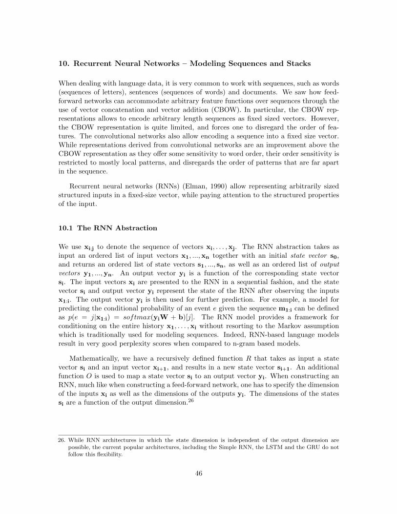
10. Recurrent Neural Networks – Modeling Sequences and Stacks

When dealing with language data, it is very common to work with sequences, such as words(sequences of letters), sentences (sequences of words) and documents. We saw how feed-forward networks can accommodate arbitrary feature functions over sequences through theuse of vector concatenation and vector addition (CBOW). In particular, the CBOW rep-resentations allows to encode arbitrary length sequences as fixed sized vectors. However,the CBOW representation is quite limited, and forces one to disregard the order of fea-tures. The convolutional networks also allow encoding a sequence into a fixed size vector.While representations derived from convolutional networks are an improvement above theCBOW representation as they offer some sensitivity to word order, their order sensitivity isrestricted to mostly local patterns, and disregards the order of patterns that are far apartin the sequence.

Recurrent neural networks (RNNs) (Elman, 1990) allow representing arbitrarily sizedstructured inputs in a fixed-size vector, while paying attention to the structured propertiesof the input.

10.1 The RNN Abstraction

We use xi:j to denote the sequence of vectors xi, . . . ,xj. The RNN abstraction takes asinput an ordered list of input vectors x1, ...,xn together with an initial state vector s0,and returns an ordered list of state vectors s1, ..., sn, as well as an ordered list of outputvectors y1, ...,yn. An output vector yi is a function of the corresponding state vectorsi. The input vectors xi are presented to the RNN in a sequential fashion, and the statevector si and output vector yi represent the state of the RNN after observing the inputsx1:i. The output vector yi is then used for further prediction. For example, a model forpredicting the conditional probability of an event e given the sequence m1:i can be definedas p(e = j|x1:i) = softmax(yiW + b)[j]. The RNN model provides a framework forconditioning on the entire history x1, . . . ,xi without resorting to the Markov assumptionwhich is traditionally used for modeling sequences. Indeed, RNN-based language modelsresult in very good perplexity scores when compared to n-gram based models.

Mathematically, we have a recursively defined function R that takes as input a statevector si and an input vector xi+1, and results in a new state vector si+1. An additionalfunction O is used to map a state vector si to an output vector yi. When constructing anRNN, much like when constructing a feed-forward network, one has to specify the dimensionof the inputs xi as well as the dimensions of the outputs yi. The dimensions of the statessi are a function of the output dimension.26

26. While RNN architectures in which the state dimension is independent of the output dimension arepossible, the current popular architectures, including the Simple RNN, the LSTM and the GRU do notfollow this flexibility.

46

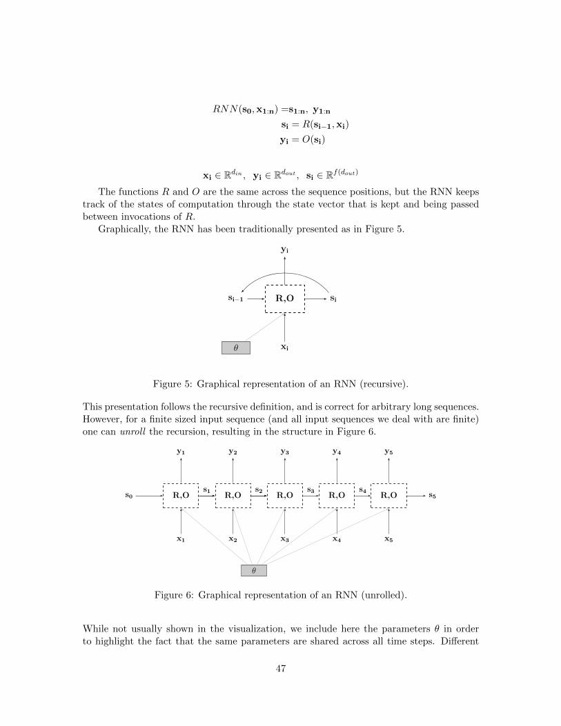
RNN(s0,x1:n) =s1:n, y1:n

si = R(si−1,xi)

yi = O(si)

xi ∈ Rdin , yi ∈ Rdout , si ∈ Rf(dout)

The functions R and O are the same across the sequence positions, but the RNN keepstrack of the states of computation through the state vector that is kept and being passedbetween invocations of R.

Graphically, the RNN has been traditionally presented as in Figure 5.

R,O

xi

yi

sisi−1

θ

Figure 5: Graphical representation of an RNN (recursive).

This presentation follows the recursive definition, and is correct for arbitrary long sequences.However, for a finite sized input sequence (and all input sequences we deal with are finite)one can unroll the recursion, resulting in the structure in Figure 6.

s0 R,O

x1

y1

R,O

x2

y2

s1R,O

x3

y3

s2

θ

R,O

x4

y4

s3R,O

x5

y5

s4 s5

Figure 6: Graphical representation of an RNN (unrolled).

While not usually shown in the visualization, we include here the parameters θ in orderto highlight the fact that the same parameters are shared across all time steps. Different

47

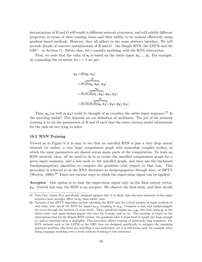
instantiations of R and O will result in different network structures, and will exhibit differentproperties in terms of their running times and their ability to be trained effectively usinggradient-based methods. However, they all adhere to the same abstract interface. We willprovide details of concrete instantiations of R and O – the Simple RNN, the LSTM and theGRU – in Section 11. Before that, let’s consider modeling with the RNN abstraction.

First, we note that the value of si is based on the entire input x1, ...,xi. For example,by expanding the recursion for i = 4 we get:

s4 =R(s3,x4)

=R(

s3︷ ︸︸ ︷R(s2,x3),x4)

=R(R(

s2︷ ︸︸ ︷R(s1,x2),x3),x4)

=R(R(R(

s1︷ ︸︸ ︷R(s0,x1),x2),x3),x4)

Thus, sn (as well as yn) could be thought of as encoding the entire input sequence.27 Isthe encoding useful? This depends on our definition of usefulness. The job of the networktraining is to set the parameters of R and O such that the state conveys useful informationfor the task we are tying to solve.

10.2 RNN Training

Viewed as in Figure 6 it is easy to see that an unrolled RNN is just a very deep neuralnetwork (or rather, a very large computation graph with somewhat complex nodes), inwhich the same parameters are shared across many parts of the computation. To train anRNN network, then, all we need to do is to create the unrolled computation graph for agiven input sequence, add a loss node to the unrolled graph, and then use the backward(backpropagation) algorithm to compute the gradients with respect to that loss. Thisprocedure is referred to in the RNN literature as backpropagation through time, or BPTT(Werbos, 1990).28 There are various ways in which the supervision signal can be applied.

Acceptor One option is to base the supervision signal only on the final output vector,yn. Viewed this way, the RNN is an acceptor. We observe the final state, and then decide

27. Note that, unless R is specifically designed against this, it is likely that the later elements of the inputsequence have stronger effect on sn than earlier ones.

28. Variants of the BPTT algorithm include unrolling the RNN only for a fixed number of input symbols ateach time: first unroll the RNN for inputs x1:k, resulting in s1:k. Compute a loss, and backpropagatethe error through the network (k steps back). Then, unroll the inputs xk+1:2k, this time using sk as theinitial state, and again backpropagate the error for k steps, and so on. This strategy is based on theobservations that for the Simple-RNN variant, the gradients after k steps tend to vanish (for large enoughk), and so omitting them is negligible. This procedure allows training of arbitrarily long sequences. ForRNN variants such as the LSTM or the GRU that are designed specifically to mitigate the vanishinggradients problem, this fixed size unrolling is less motivated, yet it is still being used, for example whendoing language modeling over a book without breaking it into sentences.

48

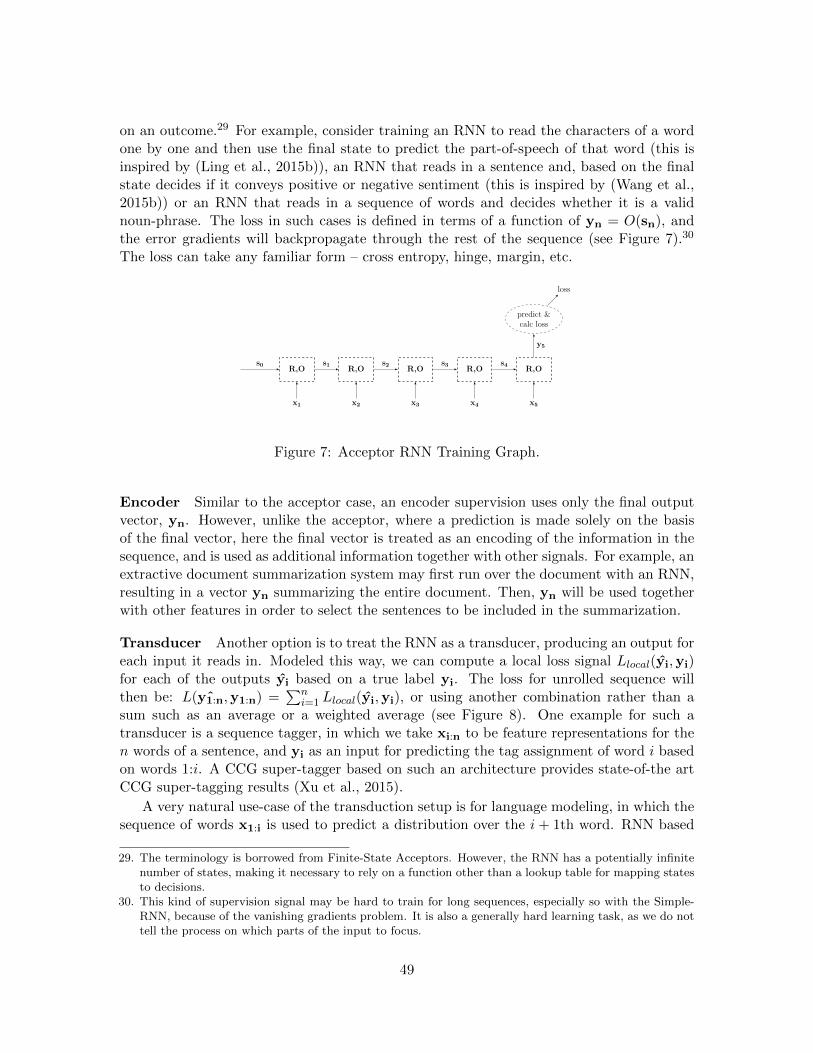
on an outcome.29 For example, consider training an RNN to read the characters of a wordone by one and then use the final state to predict the part-of-speech of that word (this isinspired by (Ling et al., 2015b)), an RNN that reads in a sentence and, based on the finalstate decides if it conveys positive or negative sentiment (this is inspired by (Wang et al.,2015b)) or an RNN that reads in a sequence of words and decides whether it is a validnoun-phrase. The loss in such cases is defined in terms of a function of yn = O(sn), andthe error gradients will backpropagate through the rest of the sequence (see Figure 7).30

The loss can take any familiar form – cross entropy, hinge, margin, etc.

R,O

x1

s0R,O

x2

s1R,O

x3

s2R,O

x4

s3R,O

x5

s4

predict &calc loss

y5

loss

Figure 7: Acceptor RNN Training Graph.

Encoder Similar to the acceptor case, an encoder supervision uses only the final outputvector, yn. However, unlike the acceptor, where a prediction is made solely on the basisof the final vector, here the final vector is treated as an encoding of the information in thesequence, and is used as additional information together with other signals. For example, anextractive document summarization system may first run over the document with an RNN,resulting in a vector yn summarizing the entire document. Then, yn will be used togetherwith other features in order to select the sentences to be included in the summarization.

Transducer Another option is to treat the RNN as a transducer, producing an output foreach input it reads in. Modeled this way, we can compute a local loss signal Llocal(yi,yi)for each of the outputs yi based on a true label yi. The loss for unrolled sequence willthen be: L( ˆy1:n,y1:n) =

∑ni=1 Llocal(yi,yi), or using another combination rather than a

sum such as an average or a weighted average (see Figure 8). One example for such atransducer is a sequence tagger, in which we take xi:n to be feature representations for then words of a sentence, and yi as an input for predicting the tag assignment of word i basedon words 1:i. A CCG super-tagger based on such an architecture provides state-of-the artCCG super-tagging results (Xu et al., 2015).

A very natural use-case of the transduction setup is for language modeling, in which thesequence of words x1:i is used to predict a distribution over the i+ 1th word. RNN based

29. The terminology is borrowed from Finite-State Acceptors. However, the RNN has a potentially infinitenumber of states, making it necessary to rely on a function other than a lookup table for mapping statesto decisions.

30. This kind of supervision signal may be hard to train for long sequences, especially so with the Simple-RNN, because of the vanishing gradients problem. It is also a generally hard learning task, as we do nottell the process on which parts of the input to focus.

49

R,O

x1

s0

predict &calc loss

y1

R,O

x2

s1

predict &calc loss

y2

R,O

x3

s2

predict &calc loss

y3

R,O

x4

s3

predict &calc loss

y4

R,O

x5

s4

predict &calc loss

y5

sum

loss

Figure 8: Transducer RNN Training Graph.

language models are shown to provide much better perplexities than traditional languagemodels (Mikolov et al., 2010; Sundermeyer, Schluter, & Ney, 2012; Mikolov, 2012).

Using RNNs as transducers allows us to relax the Markov assumption that is tradition-ally taken in language models and HMM taggers, and condition on the entire predictionhistory. The power of the ability to condition on arbitrarily long histories is demonstratedin generative character-level RNN models, in which a text is generated character by charac-ter, each character conditioning on the previous ones (Sutskever, Martens, & Hinton, 2011).The generated texts show sensitivity to properties that are not captured by n-gram languagemodels, including line lengths and nested parenthesis balancing. For a good demonstrationand analysis of the properties of RNN-based character level language models, see (Karpathy,Johnson, & Li, 2015).

Encoder - Decoder Finally, an important special case of the encoder scenario is theEncoder-Decoder framework (Cho, van Merrienboer, Bahdanau, & Bengio, 2014a; Sutskeveret al., 2014). The RNN is used to encode the sequence into a vector representation yn, andthis vector representation is then used as auxiliary input to another RNN that is used asa decoder. For example, in a machine-translation setup the first RNN encodes the sourcesentence into a vector representation yn, and then this state vector is fed into a separate(decoder) RNN that is trained to predict (using a transducer-like language modeling ob-jective) the words of the target language sentence based on the previously predicted wordsas well as yn. The supervision happens only for the decoder RNN, but the gradients arepropagated all the way back to the encoder RNN (see Figure 9).

Such an approach was shown to be surprisingly effective for Machine Translation (Sutskeveret al., 2014) using LSTM RNNs. In order for this technique to work, Sutskever et al found iteffective to input the source sentence in reverse, such that xn corresponds to the first wordof the sentence. In this way, it is easier for the second RNN to establish the relation be-tween the first word of the source sentence to the first word of the target sentence. Anotheruse-case of the encoder-decoder framework is for sequence transduction. Here, in order togenerate tags t1, . . . , tn, an encoder RNN is first used to encode the sentence x1:n into fixedsized vector. This vector is then fed as the initial state vector of another (transducer) RNN,which is used together with x1:n to predict the label ti at each position i. This approach

50

RE,OE

x1

se0RE,OE

x2

se1RE,OE

x3

se2RE,OE

x4

se3RE,OE

x5

se4 se5

RD,OD

x1

sd0

predict &calc loss

y1

RD,OD

x2

sd1

predict &calc loss

y2

RD,OD

x3

sd2

predict &calc loss

y3

RD,OD

x4

sd3

predict &calc loss

y4

RD,OD

x5

sd4

predict &calc loss

y5

sum

loss

Figure 9: Encoder-Decoder RNN Training Graph.

was used in (Filippova, Alfonseca, Colmenares, Kaiser, & Vinyals, 2015) to model sentencecompression by deletion.

10.3 Multi-layer (stacked) RNNs

RNNs can be stacked in layers, forming a grid (Hihi & Bengio, 1996). Consider k RNNs,

RNN1, . . . , RNNk, where the jth RNN has states sj1:n and outputs yj1:n. The input for the

first RNN are x1:n, while the input of the jth RNN (j ≥ 2) are the outputs of the RNN

below it, yj−11:n . The output of the entire formation is the output of the last RNN, yk

1:n.Such layered architectures are often called deep RNNs. A visual representation of a 3-layerRNN is given in Figure 10.

While it is not theoretically clear what is the additional power gained by the deeperarchitecture, it was observed empirically that deep RNNs work better than shallower oneson some tasks. In particular, Sutskever et al (2014) report that a 4-layers deep architec-ture was crucial in achieving good machine-translation performance in an encoder-decoderframework. Irsoy and Cardie (2014) also report improved results from moving from a one-layer BI-RNN to an architecture with several layers. Many other works report result usinglayered RNN architectures, but do not explicitly compare to 1-layer RNNs.

51

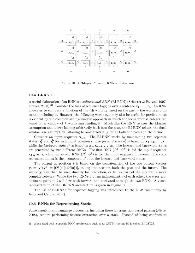
R1,O1

R2,O2

y11

s10

R3,O3

y21

s20

s30

x1

y1

y31

R1,O1

R2,O2

y12

s11

R3,O3

y22

s21

s31

x2

y2

y32

R1,O1

R2,O2

y13

s12

R3,O3

y23

s22

s32

x3

y3

y33

R1,O1

R2,O2

y14

s13

R3,O3

y24

s23

s33

x4

y4

y34

R1,O1

R2,O2

y15

s14

R3,O3

y25

s24

s34

x5

y5

y35

s15

s25

s35

Figure 10: A 3-layer (“deep”) RNN architecture.

10.4 BI-RNN

A useful elaboration of an RNN is a bidirectional-RNN (BI-RNN) (Schuster & Paliwal, 1997;Graves, 2008).31 Consider the task of sequence tagging over a sentence x1, . . . , xn. An RNNallows us to compute a function of the ith word xi based on the past – the words x1:i upto and including it. However, the following words xi:n may also be useful for prediction, asis evident by the common sliding-window approach in which the focus word is categorizedbased on a window of k words surrounding it. Much like the RNN relaxes the Markovassumption and allows looking arbitrarily back into the past, the BI-RNN relaxes the fixedwindow size assumption, allowing to look arbitrarily far at both the past and the future.

Consider an input sequence x1:n. The BI-RNN works by maintaining two separatestates, sfi and sbi for each input position i. The forward state sfi is based on x1,x2, . . . ,xi,while the backward state sbi is based on xn,xn−1, . . . ,xi. The forward and backward statesare generated by two different RNNs. The first RNN (Rf , Of ) is fed the input sequencex1:n as is, while the second RNN (Rb, Ob) is fed the input sequence in reverse. The staterepresentation si is then composed of both the forward and backward states.

The output at position i is based on the concatenation of the two output vectorsyi = [yf

i ; ybi ] = [Of (sfi );O

b(sbi )], taking into account both the past and the future. Thevector yi can then be used directly for prediction, or fed as part of the input to a morecomplex network. While the two RNNs are run independently of each other, the error gra-dients at position i will flow both forward and backward through the two RNNs. A visualrepresentation of the BI-RNN architecture is given in Figure 11.

The use of BI-RNNs for sequence tagging was introduced to the NLP community byIrsoy and Cardie (2014).

10.5 RNNs for Representing Stacks

Some algorithms in language processing, including those for transition-based parsing (Nivre,2008), require performing feature extraction over a stack. Instead of being confined to

31. When used with a specific RNN architecture such as an LSTM, the model is called BI-LSTM.

52

Rf ,Of

xthe

concat

yf1

sf0Rf ,Of

xbrown

concat

yf2

sf1Rf ,Of

xfox

concat

yf3

sf2Rf ,Of

xjumped

concat

yf4

sf3Rf ,Of

x∗

concat

yf5

sf4 sf5

Rb,Obs0sb0

yb1

Rb,Obs1sb1

yb2

Rb,Obs2sb2

yb3

Rb,Obs3sb3

yb4

Rb,Obs4sb4

yb5

sb5

ythe ybrown yfox yjumped y∗

Figure 11: BI-RNN over the sentence “the brown fox jumped .”.

looking at the k top-most elements of the stack, the RNN framework can be used to providea fixed-sized vector encoding of the entire stack.

The main intuition is that a stack is essentially a sequence, and so the stack state can berepresented by taking the stack elements and feeding them in order into an RNN, resultingin a final encoding of the entire stack. In order to do this computation efficiently (withoutperforming an O(n) stack encoding operation each time the stack changes), the RNN stateis maintained together with the stack state. If the stack was push-only, this would betrivial: whenever a new element x is pushed into the stack, the corresponding vector xwill be used together with the RNN state si in order to obtain a new state si+1. Dealingwith pop operation is more challenging, but can be solved by using the persistent-stackdata-structure (Okasaki, 1999; Goldberg, Zhao, & Huang, 2013). Persistent, or immutable,data-structures keep old versions of themselves intact when modified. The persistent stackconstruction represents a stack as a pointer to the head of a linked list. An empty stack isthe empty list. The push operation appends an element to the list, returning the new head.The pop operation then returns the parent of the head, but keeping the original list intact.From the point of view of someone who held a pointer to the previous head, the stack didnot change. A subsequent push operation will add a new child to the same node. Applyingthis procedure throughout the lifetime of the stack results in a tree, where the root is anempty stack and each path from a node to the root represents an intermediary stack state.Figure 12 provides an example of such a tree. The same process can be applied in thecomputation graph construction, creating an RNN with a tree structure instead of a chainstructure. Backpropagating the error from a given node will then affect all the elementsthat participated in the stack when the node was created, in order. Figure 13 shows thecomputation graph for the stack-RNN corresponding to the last state in Figure 12. Thismodeling approach was proposed independently by Dyer et al and Watanabe et al (Dyeret al., 2015; Watanabe & Sumita, 2015) for transition-based dependency parsing.

53

⊥ a

head

(1) push a

⊥ a b

head

(2) push b

⊥ a b c

head

(3) push c

⊥ a b

head

c

(4) pop

⊥ a b c

d

head

(5) push d

⊥ a b

head

c

d

(6) pop

⊥ a

head

b c

d

(7) pop

⊥ a b c

d

e

head

(8) push e

⊥ a b c

d

e f

head

(9) push f

Figure 12: An immutable stack construction for the sequence of operations push a; push b;push c; pop; push d; pop; pop; push e; push f.

so R,O

ya

xa

R,Osa

ya:b

xb

R,Osa:b

ya:c

xc

sa:c

R,O

sa:b

ya,b,d

xd

sa,b,d

R,O

sa

ya,e

xe

R,Osa,e

ya,e,f

xf

sa,e,f

Figure 13: The stack-RNN corresponding to the final state in Figure 12.

10.6 A Note on Reading the Literature

Unfortunately, it is often the case that inferring the exact model form from reading itsdescription in a research paper can be quite challenging. Many aspects of the models

54

are not yet standardized, and different researchers use the same terms to refer to slightlydifferent things. To list a few examples, the inputs to the RNN can be either one-hot vectors(in which case the embedding matrix is internal to the RNN) or embedded representations;The input sequence can be padded with start-of-sequence and/or end-of-sequence symbols,or not; While the output of an RNN is usually assumed to be a vector which is expectedto be fed to additional layers followed by a softmax for prediction (as is the case in thepresentation in this tutorial), some papers assume the softmax to be part of the RNN itself;In multi-layer RNN, the “state vector” can be either the output of the top-most layer, or aconcatenation of the outputs from all layers; When using the encoder-decoder framework,conditioning on the output of the encoder can be interpreted in various different ways; andso on. On top of that, the LSTM architecture described in the next section has many smallvariants, which are all referred to under the common name LSTM. Some of these choicesare made explicit in the papers, other require careful reading, and others still are not evenmentioned, or are hidden behind ambiguous figures or phrasing.

As a reader, be aware of these issues when reading and interpret model descriptions. Asa writer, be aware of these issues as well: either fully specify your model in mathematicalnotation, or refer to a different source in which the model is fully specified, if such a sourceis available. If using the default implementation from a software package without knowingthe details, be explicit of that fact and specify the software package you use. In any case,don’t rely solely on figures or natural language text when describing your model, as theseare often ambiguous.

55

11. Concrete RNN Architectures

We now turn to present three different instantiations of the abstract RNN architecturediscussed in the previous section, providing concrete definitions of the functions R and O.These are the Simple RNN (SRNN), the Long Short-Term Memory (LSTM) and the GatedRecurrent Unit (GRU).

11.1 Simple RNN

The simplest RNN formulation, known as an Elman Network or Simple-RNN (S-RNN), wasproposed by Elman (1990) and explored for use in language modeling by Mikolov (2012).The S-RNN takes the following form:

si =RSRNN (si−1,xi) = g(xiWx + si−1Ws + b)

yi =OSRNN (si) = si

si,yi ∈ Rds , xi ∈ Rdx , Wx ∈ Rdx×ds , Ws ∈ Rds×ds , b ∈ Rds

That is, the state at position i is a linear combination of the input at position i andthe previous state, passed through a non-linear activation (commonly tanh or ReLU). Theoutput at position i is the same as the hidden state in that position.32

In spite of its simplicity, the Simple RNN provides strong results for sequence tagging(Xu et al., 2015) as well as language modeling. For comprehensive discussion on usingSimple RNNs for language modeling, see the PhD thesis by Mikolov (2012).

11.2 LSTM

The S-RNN is hard to train effectively because of the vanishing gradients problem. Errorsignals (gradients) in later steps in the sequence diminish quickly in the back-propagationprocess, and do not reach earlier input signals, making it hard for the S-RNN to capturelong-range dependencies. The Long Short-Term Memory (LSTM) architecture (Hochreiter& Schmidhuber, 1997) was designed to solve the vanishing gradients problem. The mainidea behind the LSTM is to introduce as part of the state representation also “memorycells” (a vector) that can preserve gradients across time. Access to the memory cells iscontrolled by gating components – smooth mathematical functions that simulate logicalgates. At each input state, a gate is used to decide how much of the new input should bewritten to the memory cell, and how much of the current content of the memory cell shouldbe forgotten. Concretely, a gate g ∈ [0, 1]n is a vector of values in the range [0, 1] that ismultiplied component-wise with another vector v ∈ Rn, and the result is then added toanother vector. The values of g are designed to be close to either 0 or 1, i.e. by using asigmoid function. Indices in v corresponding to near-one values in g are allowed to pass,while those corresponding to near-zero values are blocked.

32. Some authors treat the output at position i as a more complicated function of the state. In our presen-tation, such further transformation of the output are not considered part of the RNN, but as separatecomputations that are applied to the RNNs output. The distinction between the state and the outputare needed for the LSTM architecture, in which not all of the state is observed outside of the RNN.

56

Mathematically, the LSTM architecture is defined as:33

sj = RLSTM (sj−1,xj) =[cj; hj]

cj =cj−1 � f + g � i

hj = tanh(cj)� o

i =σ(xjWxi + hj−1Whi)

f =σ(xjWxf + hj−1Whf )

o =σ(xjWxo + hj−1Who)

g = tanh(xjWxg + hj−1Whg)

yj = OLSTM (sj) =hj

sj ∈ R2·dh , xi ∈ Rdx , cj,hj, i, f ,o,g ∈ Rdh , Wx◦ ∈ Rdx×dh , Wh◦ ∈ Rdh×dh ,

The symbol � is used to denote component-wise product. The state at time j is com-posed of two vectors, cj and hj, where cj is the memory component and hj is the output,or state, component. There are three gates, i, f and o, controlling for input, forget andoutput. The gate values are computed based on linear combinations of the current inputxj and the previous state hj−1, passed through a sigmoid activation function. An updatecandidate g is computed as a linear combination of xj and hj−1, passed through a tanhactivation function. The memory cj is then updated: the forget gate controls how muchof the previous memory to keep (cj−1 � f), and the input gate controls how much of theproposed update to keep (g � i). Finally, the value of hj (which is also the output yj) isdetermined based on the content of the memory cj, passed through a tanh non-linearityand controlled by the output gate. The gating mechanisms allow for gradients related tothe memory part cj to stay high across very long time ranges.

For further discussion on the LSTM architecture see the PhD thesis by Alex Graves(2008), as well as Chris Olah’s description.34 For an analysis of the behavior of an LSTMwhen used as a character-level language model, see (Karpathy et al., 2015).

LSTMs are currently the most successful type of RNN architecture, and they are re-sponsible for many state-of-the-art sequence modeling results. The main competitor of theLSTM-RNN is the GRU, to be discussed next.

Practical Considerations When training LSTM networks, Jozefowicz et al (2015) stronglyrecommend to always initialize the bias term of the forget gate to be close to one. Whenapplying dropout to an RNN with an LSTM, Zaremba et al (2014) found out that it is

33. There are many variants on the LSTM architecture presented here. For example, forget gates were notpart of the original proposal in (Hochreiter & Schmidhuber, 1997), but are shown to be an importantpart of the architecture. Other variants include peephole connections and gate-tying. For an overviewand comprehensive empirical comparison of various LSTM architectures see (Greff, Srivastava, Koutnık,Steunebrink, & Schmidhuber, 2015).

34. http://colah.github.io/posts/2015-08-Understanding-LSTMs/

57

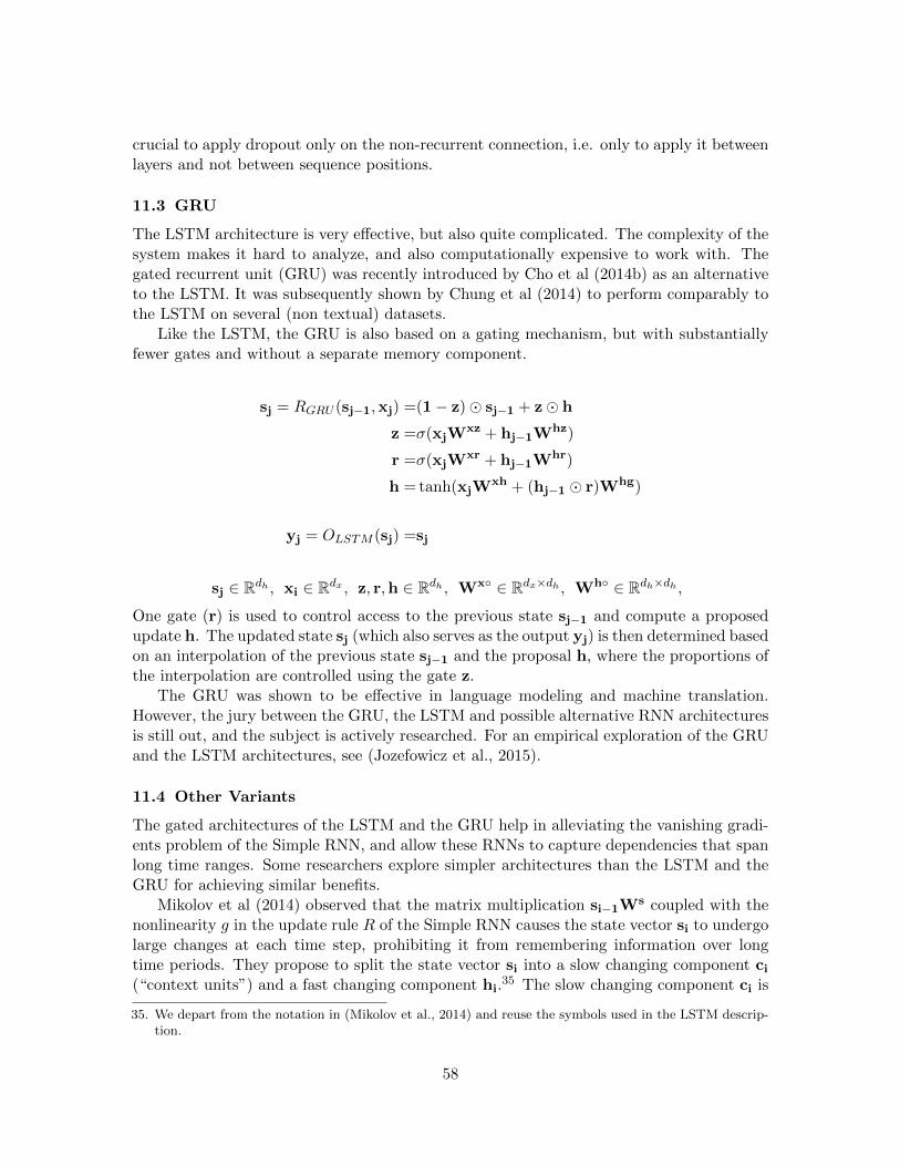
crucial to apply dropout only on the non-recurrent connection, i.e. only to apply it betweenlayers and not between sequence positions.

11.3 GRU

The LSTM architecture is very effective, but also quite complicated. The complexity of thesystem makes it hard to analyze, and also computationally expensive to work with. Thegated recurrent unit (GRU) was recently introduced by Cho et al (2014b) as an alternativeto the LSTM. It was subsequently shown by Chung et al (2014) to perform comparably tothe LSTM on several (non textual) datasets.

Like the LSTM, the GRU is also based on a gating mechanism, but with substantiallyfewer gates and without a separate memory component.

sj = RGRU (sj−1,xj) =(1− z)� sj−1 + z� h

z =σ(xjWxz + hj−1Whz)

r =σ(xjWxr + hj−1Whr)

h = tanh(xjWxh + (hj−1 � r)Whg)

yj = OLSTM (sj) =sj

sj ∈ Rdh , xi ∈ Rdx , z, r,h ∈ Rdh , Wx◦ ∈ Rdx×dh , Wh◦ ∈ Rdh×dh ,

One gate (r) is used to control access to the previous state sj−1 and compute a proposedupdate h. The updated state sj (which also serves as the output yj) is then determined basedon an interpolation of the previous state sj−1 and the proposal h, where the proportions ofthe interpolation are controlled using the gate z.

The GRU was shown to be effective in language modeling and machine translation.However, the jury between the GRU, the LSTM and possible alternative RNN architecturesis still out, and the subject is actively researched. For an empirical exploration of the GRUand the LSTM architectures, see (Jozefowicz et al., 2015).

11.4 Other Variants

The gated architectures of the LSTM and the GRU help in alleviating the vanishing gradi-ents problem of the Simple RNN, and allow these RNNs to capture dependencies that spanlong time ranges. Some researchers explore simpler architectures than the LSTM and theGRU for achieving similar benefits.

Mikolov et al (2014) observed that the matrix multiplication si−1Ws coupled with thenonlinearity g in the update rule R of the Simple RNN causes the state vector si to undergolarge changes at each time step, prohibiting it from remembering information over longtime periods. They propose to split the state vector si into a slow changing component ci(“context units”) and a fast changing component hi.

35 The slow changing component ci is

35. We depart from the notation in (Mikolov et al., 2014) and reuse the symbols used in the LSTM descrip-tion.

58

updated according to a linear interpolation of the input and the previous component: ci =(1− α)xiW

x1 + αci−1, where α ∈ (0, 1). This update allows ci to accumulate the previousinputs. The fast changing component hi is updated similarly to the Simple RNN updaterule, but changed to take ci into account as well:36 hi = σ(xiW

x2 + hi−1Wh + ciWc).

Finally, the output yi is the concatenation of the slow and the fast changing parts of thestate: yi = [ci; hi]. Mikolov et al demonstrate that this architecture provides competitiveperplexities to the much more complex LSTM on language modeling tasks.

The approach of Mikolov et al can be interpreted as constraining the block of the matrixWs in the S-RNN corresponding to ci to be a multiply of the identity matrix (see Mikolovet al (2014) for the details). Le et al (Le, Jaitly, & Hinton, 2015) propose an even simplerapproach: set the activation function of the S-RNN to a ReLU, and initialize the biases bas zeroes and the matrix Ws as the identify matrix. This causes an untrained RNN to copythe previous state to the current state, add the effect of the current input xi and set thenegative values to zero. After setting this initial bias towards state copying, the trainingprocedure allows Ws to change freely. Le et al demonstrate that this simple modificationmakes the S-RNN comparable to an LSTM with the same number of parameters on severaltasks, including language modeling.

36. The update rule diverges from the S-RNN update rule also by fixing the non-linearity to be a sigmoidfunction, and by not using a bias term. However, these changes are not discussed as central to theproposal.

59

12. Modeling Trees – Recursive Neural Networks

The RNN is very useful for modeling sequences. In language processing, it is often naturaland desirable to work with tree structures. The trees can be syntactic trees, discourse trees,or even trees representing the sentiment expressed by various parts of a sentence (Socheret al., 2013). We may want to predict values based on specific tree nodes, predict valuesbased on the root nodes, or assign a quality score to a complete tree or part of a tree. Inother cases, we may not care about the tree structure directly but rather reason about spansin the sentence. In such cases, the tree is merely used as a backbone structure which helpguide the encoding process of the sequence into a fixed size vector.

The recursive neural network (RecNN) abstraction (Pollack, 1990), popularized in NLPby Richard Socher and colleagues (Socher, Manning, & Ng, 2010; Socher, Lin, Ng, & Man-ning, 2011; Socher et al., 2013; Socher, 2014) is a generalization of the RNN from sequencesto (binary) trees.37

Much like the RNN encodes each sentence prefix as a state vector, the RecNN encodeseach tree-node as a state vector in Rd. We can then use these state vectors either to predictvalues of the corresponding nodes, assign quality values to each node, or as a semanticrepresentation of the spans rooted at the nodes.

The main intuition behind the recursive neural networks is that each subtree is repre-sented as a d dimensional vector, and the representation of a node p with children c1 and c2

is a function of the representation of the nodes: vec(p) = f(vec(c1), vec(c2)), where f is acomposition function taking two d-dimensional vectors and returning a single d-dimensionalvector. Much like the RNN state si is used to encode the entire sequence x1 : i, the RecNNstate associated with a tree node p encodes the entire subtree rooted at p. See Figure 14for an illustration.

12.1 Formal Definition

Consider a binary parse tree T over an n-word sentence. As a reminder, an ordered,unlabeled tree over a string x1, . . . , xn can be represented as a unique set of triplets (i, k, j),s.t. i ≤ k ≤ j. Each such triplet indicates that a node spanning words xi:j is parent of thenodes spanning xi:k and xk+1:j . Triplets of the form (i, i, i) correspond to terminal symbolsat the tree leaves (the words xi). Moving from the unlabeled case to the labeled one, we canrepresent a tree as a set of 6-tuples (A→ B,C, i, k, j), whereas i, k and j indicate the spansas before, and A, B and C are the node labels of of the nodes spanning xi:j , xi:k and xk+1:j

respectively. Here, leaf nodes have the form (A → A,A, i, i, i), where A is a pre-terminalsymbol. We refer to such tuples as production rules. For an example, consider the syntactictree for the sentence “the boy saw her duck”.

37. While presented in terms of binary parse trees, the concepts easily transfer to general recursively-defineddata structures, with the major technical challenge is the definition of an effective form for R, thecombination function.

60

V = NP1 =

combine

VP =NP2 =

combine

S =

Figure 14: Illustration of a recursive neural network. The representations of V and NP1

are combined to form the representation of VP. The representations of VP andNP2 are then combined to form the representation of S.

S

VP

NP

Noun

duck

Det

her

Verb

saw

NP

Noun

boy

Det

the

Its corresponding unlabeled and labeled representations are :

Unlabeled Labeled Corresponding Span

(1,1,1) (Det, Det, Det, 1, 1, 1) x1:1 the(2,2,2) (Noun, Noun, Noun, 2, 2, 2) x2:2 boy(3,3,3) (Verb, Verb, Verb, 3, 3, 3) saw(4,4,4) (Det, Det, Det, 4, 4, 4) her(5,5,5) (Noun, Noun, Noun, 5, 5, 5) duck(4,4,5) (NP, Det, Noun, 4, 4, 5) her duck(3,3,5) (VP, Verb, NP, 3, 3, 5) saw her duck(1,1,2) (NP, Det, Noun, 1, 1, 2) the boy(1,2,5) (S, NP, VP, 1, 2, 5) the boy saw her duck

The set of production rules above can be uniquely converted to a set tree nodes qAi:j(indicating a node with symbol A over the span xi:j) by simply ignoring the elements

61

(B,C, k) in each production rule. We are now in position to define the Recursive NeuralNetwork.

A Recursive Neural Network (RecNN) is a function that takes as input a parse treeover an n-word sentence x1, . . . , xn. Each of the sentence’s words is represented as a d-dimensional vector xi, and the tree is represented as a set T of production rules (A →B,C, i, j, k). Denote the nodes of T by qAi:j . The RecNN returns as output a correspond-

ing set of inside state vectors sAi:j, where each inside state vector sAi:j ∈ Rd represents the

corresponding tree node qAi:j , and encodes the entire structure rooted at that node. Likethe sequence RNN, the tree shaped RecNN is defined recursively using a function R, wherethe inside vector of a given node is defined as a function of the inside vectors of its directchildren.38 Formally:

RecNN(x1, . . . , xn, T ) ={sAi:j ∈ Rd | qAi:j ∈ T }sAi:i =v(xi)

sAi:j =R(A,B,C, sBi:k, sCk+1:j) qBi:k ∈ T , qCk+1:j ∈ T

The function R usually takes the form of a simple linear transformation, which may ormay not be followed by a non-linear activation function g:

R(A,B,C, sBi:k, sCk+1:j) = g([sBi:k; sCk+1:j]W)

This formulation of R ignores the tree labels, using the same matrix W ∈ R2d×d for allcombinations. This may be a useful formulation in case the node labels do not exist (e.g.when the tree does not represent a syntactic structure with clearly defined labels) or whenthey are unreliable. However, if the labels are available, it is generally useful to include themin the composition function. One approach would be to introduce label embeddings v(A)mapping each non-terminal symbol to a dnt dimensional vector, and change R to includethe embedded symbols in the combination function:

R(A,B,C, sBi:k, sCk+1:j) = g([sBi:k; sCk+1:j; v(A); v(B)]W)

(here, W ∈ R2d+2dnt×d). Such approach is taken by (Qian, Tian, Huang, Liu, Zhu, &Zhu, 2015). An alternative approach, due to (Socher et al., 2013) is to untie the weightsaccording to the non-terminals, using a different composition matrix for each B,C pair ofsymbols:39

R(A,B,C, sBi:k, sCk+1:j) = g([sBi:k; sCk+1:j]W

BC)

38. Le and Zuidema (2014) extend the RecNN definition such that each node has, in addition to its insidestate vector, also an outside state vector representing the entire structure around the subtree rootedat that node. Their formulation is based on the recursive computation of the classic inside-outsidealgorithm, and can be thought of as the BI-RNN counterpart of the tree RecNN. For details, see (Le &Zuidema, 2014).

39. While not explored in the literature, a trivial extension would condition the transformation matrix alsoon A.

62

This formulation is useful when the number of non-terminal symbols (or the number ofpossible symbol combinations) is relatively small, as is usually the case with phrase-structureparse trees. A similar model was also used by (Hashimoto et al., 2013) to encode subtreesin semantic-relation classification task.

12.2 Extensions and Variations

As all of the definitions of R above suffer from the vanishing gradients problem of theSimple RNN, several authors sought to replace it with functions inspired by the Long Short-Term Memory (LSTM) gated architecture, resulting in Tree-shaped LSTMs (Tai, Socher, &Manning, 2015; Zhu, Sobhani, & Guo, 2015b). The question of optimal tree representationis still very much an open research question, and the vast space of possible combinationfunctions R is yet to be explored. Other proposed variants on tree-structured RNNs includesa recursive matrix-vector model (Socher, Huval, Manning, & Ng, 2012) and recursive neuraltensor network (Socher et al., 2013). In the first variant, each word is represented as acombination of a vector and a matrix, where the vector defines the word’s static semanticcontent as before, while the matrix acts as a learned “operator” for the word, allowingmore subtle semantic compositions than the addition and weighted averaging implied bythe concatenation followed by linear transformation function. In the second variant, wordsare associated with vectors as usual, but the composition function becomes more expressiveby basing it on tensor instead of matrix operations.

12.3 Training Recursive Neural Networks

The training procedure for a recursive neural network follows the same recipe as trainingother forms of networks: define a loss, spell out the computation graph, compute gradientsusing backpropagation40, and train the parameters using SGD.

With regard to the loss function, similar to the sequence RNN one can associate a losseither with the root of the tree, with any given node, or with a set of nodes, in which casethe individual node’s losses are combined, usually by summation. The loss function is basedon the labeled training data which associates a label or other quantity with different treenodes.

Additionally, one can treat the RecNN as an Encoder, whereas the inside-vector associ-ated with a node is taken to be an encoding of the tree rooted at that node. The encodingcan potentially be sensitive to arbitrary properties of the structure. The vector is thenpassed as input to another network.

For further discussion on recursive neural networks and their use in natural languagetasks, refer to the PhD thesis of Richard Socher (2014).

40. Before the introduction of the computation graph abstraction, the specific backpropagation procedurefor computing the gradients in a RecNN as defined above was referred to as the Back-propagation troughStructure (BPTS) algorithm (Goller & Kuchler, 1996).

63

13. Conclusions

Neural networks are powerful learners, providing opportunities ranging from non-linearclassification to non-Markovian modeling of sequences and trees. We hope that this expo-sition help NLP researchers to incorporate neural network models in their work and takeadvantage of their power.

References

Adel, H., Vu, N. T., & Schultz, T. (2013). Combination of Recurrent Neural Networks andFactored Language Models for Code-Switching Language Modeling. In Proceedingsof the 51st Annual Meeting of the Association for Computational Linguistics (Vol-ume 2: Short Papers), pp. 206–211, Sofia, Bulgaria. Association for ComputationalLinguistics.

Ando, R., & Zhang, T. (2005a). A High-Performance Semi-Supervised Learning Methodfor Text Chunking. In Proceedings of the 43rd Annual Meeting of the Association forComputational Linguistics (ACL’05), pp. 1–9, Ann Arbor, Michigan. Association forComputational Linguistics.

Ando, R. K., & Zhang, T. (2005b). A framework for learning predictive structures frommultiple tasks and unlabeled data. The Journal of Machine Learning Research, 6,1817–1853.

Auli, M., Galley, M., Quirk, C., & Zweig, G. (2013). Joint Language and Translation Mod-eling with Recurrent Neural Networks. In Proceedings of the 2013 Conference onEmpirical Methods in Natural Language Processing, pp. 1044–1054, Seattle, Washing-ton, USA. Association for Computational Linguistics.

Auli, M., & Gao, J. (2014). Decoder Integration and Expected BLEU Training for RecurrentNeural Network Language Models. In Proceedings of the 52nd Annual Meeting of theAssociation for Computational Linguistics (Volume 2: Short Papers), pp. 136–142,Baltimore, Maryland. Association for Computational Linguistics.

Ballesteros, M., Dyer, C., & Smith, N. A. (2015). Improved Transition-based Parsing byModeling Characters instead of Words with LSTMs. In Proceedings of the 2015 Con-ference on Empirical Methods in Natural Language Processing, pp. 349–359, Lisbon,Portugal. Association for Computational Linguistics.

Bansal, M., Gimpel, K., & Livescu, K. (2014). Tailoring Continuous Word Representationsfor Dependency Parsing. In Proceedings of the 52nd Annual Meeting of the Associationfor Computational Linguistics (Volume 2: Short Papers), pp. 809–815, Baltimore,Maryland. Association for Computational Linguistics.

Baydin, A. G., Pearlmutter, B. A., Radul, A. A., & Siskind, J. M. (2015). Automaticdifferentiation in machine learning: a survey. arXiv:1502.05767 [cs].

Bengio, Y. (2012). Practical recommendations for gradient-based training of deep architec-tures. arXiv:1206.5533 [cs].

Bengio, Y., Ducharme, R., Vincent, P., & Janvin, C. (2003). A Neural Probabilistic Lan-guage Model. J. Mach. Learn. Res., 3, 1137–1155.

64

Bengio, Y., Goodfellow, I. J., & Courville, A. (2015). Deep Learning. Book in preparationfor MIT Press.

Bitvai, Z., & Cohn, T. (2015). Non-Linear Text Regression with a Deep ConvolutionalNeural Network. In Proceedings of the 53rd Annual Meeting of the Association forComputational Linguistics and the 7th International Joint Conference on Natural Lan-guage Processing (Volume 2: Short Papers), pp. 180–185, Beijing, China. Associationfor Computational Linguistics.

Botha, J. A., & Blunsom, P. (2014). Compositional Morphology for Word Representationsand Language Modelling. In Proceedings of the 31st International Conference onMachine Learning (ICML), Beijing, China. *Award for best application paper*.

Bottou, L. (2012). Stochastic gradient descent tricks. In Neural Networks: Tricks of theTrade, pp. 421–436. Springer.

Charniak, E., & Johnson, M. (2005). Coarse-to-Fine n-Best Parsing and MaxEnt Discrim-inative Reranking. In Proceedings of the 43rd Annual Meeting of the Association forComputational Linguistics (ACL’05), pp. 173–180, Ann Arbor, Michigan. Associationfor Computational Linguistics.

Chen, D., & Manning, C. (2014). A Fast and Accurate Dependency Parser using NeuralNetworks. In Proceedings of the 2014 Conference on Empirical Methods in NaturalLanguage Processing (EMNLP), pp. 740–750, Doha, Qatar. Association for Compu-tational Linguistics.

Chen, Y., Xu, L., Liu, K., Zeng, D., & Zhao, J. (2015). Event Extraction via DynamicMulti-Pooling Convolutional Neural Networks. In Proceedings of the 53rd AnnualMeeting of the Association for Computational Linguistics and the 7th InternationalJoint Conference on Natural Language Processing (Volume 1: Long Papers), pp. 167–176, Beijing, China. Association for Computational Linguistics.

Cho, K., van Merrienboer, B., Bahdanau, D., & Bengio, Y. (2014a). On the Properties ofNeural Machine Translation: Encoder–Decoder Approaches. In Proceedings of SSST-8, Eighth Workshop on Syntax, Semantics and Structure in Statistical Translation,pp. 103–111, Doha, Qatar. Association for Computational Linguistics.

Cho, K., van Merrienboer, B., Gulcehre, C., Bahdanau, D., Bougares, F., Schwenk, H., &Bengio, Y. (2014b). Learning Phrase Representations using RNN Encoder–Decoder forStatistical Machine Translation. In Proceedings of the 2014 Conference on EmpiricalMethods in Natural Language Processing (EMNLP), pp. 1724–1734, Doha, Qatar.Association for Computational Linguistics.

Chrupala, G. (2014). Normalizing tweets with edit scripts and recurrent neural embeddings.In Proceedings of the 52nd Annual Meeting of the Association for Computational Lin-guistics (Volume 2: Short Papers), pp. 680–686, Baltimore, Maryland. Association forComputational Linguistics.

Chung, J., Gulcehre, C., Cho, K., & Bengio, Y. (2014). Empirical Evaluation of GatedRecurrent Neural Networks on Sequence Modeling. arXiv:1412.3555 [cs].

Collins, M. (2002). Discriminative Training Methods for Hidden Markov Models: Theoryand Experiments with Perceptron Algorithms. In Proceedings of the 2002 Confer-

65

ence on Empirical Methods in Natural Language Processing, pp. 1–8. Association forComputational Linguistics.

Collins, M., & Koo, T. (2005). Discriminative Reranking for Natural Language Parsing.Computational Linguistics, 31 (1), 25–70.

Collobert, R., & Weston, J. (2008). A unified architecture for natural language processing:Deep neural networks with multitask learning. In Proceedings of the 25th internationalconference on Machine learning, pp. 160–167. ACM.

Collobert, R., Weston, J., Bottou, L., Karlen, M., Kavukcuoglu, K., & Kuksa, P. (2011).Natural language processing (almost) from scratch. The Journal of Machine LearningResearch, 12, 2493–2537.

Crammer, K., & Singer, Y. (2002). On the algorithmic implementation of multiclass kernel-based vector machines. The Journal of Machine Learning Research, 2, 265–292.

Creutz, M., & Lagus, K. (2007). Unsupervised Models for Morpheme Segmentation andMorphology Learning. ACM Trans. Speech Lang. Process., 4 (1), 3:1–3:34.

Cybenko, G. (1989). Approximation by superpositions of a sigmoidal function. Mathematicsof Control, Signals and Systems, 2 (4), 303–314.

Dahl, G., Sainath, T., & Hinton, G. (2013). Improving deep neural networks for LVCSRusing rectified linear units and dropout. In 2013 IEEE International Conference onAcoustics, Speech and Signal Processing (ICASSP), pp. 8609–8613.

de Gispert, A., Iglesias, G., & Byrne, B. (2015). Fast and Accurate Preordering for SMTusing Neural Networks. In Proceedings of the 2015 Conference of the North AmericanChapter of the Association for Computational Linguistics: Human Language Technolo-gies, pp. 1012–1017, Denver, Colorado. Association for Computational Linguistics.

Dong, L., Wei, F., Tan, C., Tang, D., Zhou, M., & Xu, K. (2014). Adaptive Recursive NeuralNetwork for Target-dependent Twitter Sentiment Classification. In Proceedings ofthe 52nd Annual Meeting of the Association for Computational Linguistics (Volume2: Short Papers), pp. 49–54, Baltimore, Maryland. Association for ComputationalLinguistics.

Dong, L., Wei, F., Zhou, M., & Xu, K. (2015). Question Answering over Freebase withMulti-Column Convolutional Neural Networks. In Proceedings of the 53rd AnnualMeeting of the Association for Computational Linguistics and the 7th InternationalJoint Conference on Natural Language Processing (Volume 1: Long Papers), pp. 260–269, Beijing, China. Association for Computational Linguistics.

dos Santos, C., & Gatti, M. (2014). Deep Convolutional Neural Networks for SentimentAnalysis of Short Texts. In Proceedings of COLING 2014, the 25th International Con-ference on Computational Linguistics: Technical Papers, pp. 69–78, Dublin, Ireland.Dublin City University and Association for Computational Linguistics.

dos Santos, C., Xiang, B., & Zhou, B. (2015). Classifying Relations by Ranking withConvolutional Neural Networks. In Proceedings of the 53rd Annual Meeting of theAssociation for Computational Linguistics and the 7th International Joint Confer-ence on Natural Language Processing (Volume 1: Long Papers), pp. 626–634, Beijing,China. Association for Computational Linguistics.

66

Duchi, J., Hazan, E., & Singer, Y. (2011). Adaptive subgradient methods for online learningand stochastic optimization. The Journal of Machine Learning Research, 12, 2121–2159.

Duh, K., Neubig, G., Sudoh, K., & Tsukada, H. (2013). Adaptation Data Selection us-ing Neural Language Models: Experiments in Machine Translation. In Proceedingsof the 51st Annual Meeting of the Association for Computational Linguistics (Vol-ume 2: Short Papers), pp. 678–683, Sofia, Bulgaria. Association for ComputationalLinguistics.

Durrett, G., & Klein, D. (2015). Neural CRF Parsing. In Proceedings of the 53rd AnnualMeeting of the Association for Computational Linguistics and the 7th InternationalJoint Conference on Natural Language Processing (Volume 1: Long Papers), pp. 302–312, Beijing, China. Association for Computational Linguistics.

Dyer, C., Ballesteros, M., Ling, W., Matthews, A., & Smith, N. A. (2015). Transition-Based Dependency Parsing with Stack Long Short-Term Memory. In Proceedings ofthe 53rd Annual Meeting of the Association for Computational Linguistics and the7th International Joint Conference on Natural Language Processing (Volume 1: LongPapers), pp. 334–343, Beijing, China. Association for Computational Linguistics.

Elman, J. L. (1990). Finding Structure in Time. Cognitive Science, 14 (2), 179–211.

Faruqui, M., & Dyer, C. (2014). Improving Vector Space Word Representations Using Mul-tilingual Correlation. In Proceedings of the 14th Conference of the European Chapterof the Association for Computational Linguistics, pp. 462–471, Gothenburg, Sweden.Association for Computational Linguistics.

Filippova, K., Alfonseca, E., Colmenares, C. A., Kaiser, L., & Vinyals, O. (2015). SentenceCompression by Deletion with LSTMs. In Proceedings of the 2015 Conference onEmpirical Methods in Natural Language Processing, pp. 360–368, Lisbon, Portugal.Association for Computational Linguistics.

Gal, Y., & Ghahramani, Z. (2015). Dropout as a Bayesian Approximation: RepresentingModel Uncertainty in Deep Learning. arXiv:1506.02142 [cs, stat].

Gao, J., Pantel, P., Gamon, M., He, X., & Deng, L. (2014). Modeling Interestingness withDeep Neural Networks. In Proceedings of the 2014 Conference on Empirical Methodsin Natural Language Processing (EMNLP), pp. 2–13, Doha, Qatar. Association forComputational Linguistics.

Gimenez, J., & Marquez, L. (2004). SVMTool: A general POS tagger generator based onSupport Vector Machines. In Proceedings of the 4th LREC, Lisbon, Portugal.

Glorot, X., & Bengio, Y. (2010). Understanding the difficulty of training deep feedforwardneural networks. In International conference on artificial intelligence and statistics,pp. 249–256.

Glorot, X., Bordes, A., & Bengio, Y. (2011). Deep sparse rectifier neural networks. InInternational Conference on Artificial Intelligence and Statistics, pp. 315–323.

Goldberg, Y., & Elhadad, M. (2010). An Efficient Algorithm for Easy-First Non-DirectionalDependency Parsing. In Human Language Technologies: The 2010 Annual Conference

67

of the North American Chapter of the Association for Computational Linguistics, pp.742–750, Los Angeles, California. Association for Computational Linguistics.

Goldberg, Y., & Levy, O. (2014). word2vec Explained: deriving Mikolov et al.’s negative-sampling word-embedding method. arXiv:1402.3722 [cs, stat].

Goldberg, Y., & Nivre, J. (2013). Training Deterministic Parsers with Non-DeterministicOracles. Transactions of the Association for Computational Linguistics, 1 (0), 403–414.

Goldberg, Y., Zhao, K., & Huang, L. (2013). Efficient Implementation of Beam-SearchIncremental Parsers. In Proceedings of the 51st Annual Meeting of the Association forComputational Linguistics (Volume 2: Short Papers), pp. 628–633, Sofia, Bulgaria.Association for Computational Linguistics.

Goller, C., & Kuchler, A. (1996). Learning Task-Dependent Distributed Representationsby Backpropagation Through Structure. In In Proc. of the ICNN-96, pp. 347–352.IEEE.

Graves, A. (2008). Supervised sequence labelling with recurrent neural networks. Ph.D.thesis, Technische Universitat Munchen.

Greff, K., Srivastava, R. K., Koutnık, J., Steunebrink, B. R., & Schmidhuber, J. (2015).LSTM: A Search Space Odyssey. arXiv:1503.04069 [cs].

Hal Daume III, Langford, J., & Marcu, D. (2009). Search-based Structured Prediction.Machine Learning Journal (MLJ).

Harris, Z. (1954). Distributional Structure. Word, 10 (23), 146–162.

Hashimoto, K., Miwa, M., Tsuruoka, Y., & Chikayama, T. (2013). Simple Customizationof Recursive Neural Networks for Semantic Relation Classification. In Proceedingsof the 2013 Conference on Empirical Methods in Natural Language Processing, pp.1372–1376, Seattle, Washington, USA. Association for Computational Linguistics.

He, K., Zhang, X., Ren, S., & Sun, J. (2015). Delving Deep into Rectifiers: SurpassingHuman-Level Performance on ImageNet Classification. arXiv:1502.01852 [cs].

Henderson, M., Thomson, B., & Young, S. (2013). Deep Neural Network Approach for theDialog State Tracking Challenge. In Proceedings of the SIGDIAL 2013 Conference,pp. 467–471, Metz, France. Association for Computational Linguistics.

Hermann, K. M., & Blunsom, P. (2013). The Role of Syntax in Vector Space Models ofCompositional Semantics. In Proceedings of the 51st Annual Meeting of the Asso-ciation for Computational Linguistics (Volume 1: Long Papers), pp. 894–904, Sofia,Bulgaria. Association for Computational Linguistics.

Hermann, K. M., & Blunsom, P. (2014). Multilingual Models for Compositional DistributedSemantics. In Proceedings of the 52nd Annual Meeting of the Association for Com-putational Linguistics (Volume 1: Long Papers), pp. 58–68, Baltimore, Maryland.Association for Computational Linguistics.

Hihi, S. E., & Bengio, Y. (1996). Hierarchical Recurrent Neural Networks for Long-TermDependencies. In Touretzky, D. S., Mozer, M. C., & Hasselmo, M. E. (Eds.), Advancesin Neural Information Processing Systems 8, pp. 493–499. MIT Press.

68

Hinton, G. E., Srivastava, N., Krizhevsky, A., Sutskever, I., & Salakhutdinov, R. R.(2012). Improving neural networks by preventing co-adaptation of feature detectors.arXiv:1207.0580 [cs].

Hochreiter, S., & Schmidhuber, J. (1997). Long short-term memory. Neural computation,9 (8), 1735–1780.

Hornik, K., Stinchcombe, M., & White, H. (1989). Multilayer feedforward networks areuniversal approximators. Neural Networks, 2 (5), 359–366.

Irsoy, O., & Cardie, C. (2014). Opinion Mining with Deep Recurrent Neural Networks.In Proceedings of the 2014 Conference on Empirical Methods in Natural LanguageProcessing (EMNLP), pp. 720–728, Doha, Qatar. Association for Computational Lin-guistics.

Iyyer, M., Boyd-Graber, J., Claudino, L., Socher, R., & Daume III, H. (2014a). A NeuralNetwork for Factoid Question Answering over Paragraphs. In Proceedings of the 2014Conference on Empirical Methods in Natural Language Processing (EMNLP), pp.633–644, Doha, Qatar. Association for Computational Linguistics.

Iyyer, M., Enns, P., Boyd-Graber, J., & Resnik, P. (2014b). Political Ideology DetectionUsing Recursive Neural Networks. In Proceedings of the 52nd Annual Meeting of theAssociation for Computational Linguistics (Volume 1: Long Papers), pp. 1113–1122,Baltimore, Maryland. Association for Computational Linguistics.

Iyyer, M., Manjunatha, V., Boyd-Graber, J., & Daume III, H. (2015). Deep UnorderedComposition Rivals Syntactic Methods for Text Classification. In Proceedings of the53rd Annual Meeting of the Association for Computational Linguistics and the 7thInternational Joint Conference on Natural Language Processing (Volume 1: Long Pa-pers), pp. 1681–1691, Beijing, China. Association for Computational Linguistics.

Johnson, R., & Zhang, T. (2014). Effective Use of Word Order for Text Categorization withConvolutional Neural Networks. arXiv:1412.1058 [cs, stat].

Johnson, R., & Zhang, T. (2015). Effective Use of Word Order for Text Categorization withConvolutional Neural Networks. In Proceedings of the 2015 Conference of the NorthAmerican Chapter of the Association for Computational Linguistics: Human Lan-guage Technologies, pp. 103–112, Denver, Colorado. Association for ComputationalLinguistics.

Jozefowicz, R., Zaremba, W., & Sutskever, I. (2015). An Empirical Exploration of Recur-rent Network Architectures. In Proceedings of the 32nd International Conference onMachine Learning (ICML-15), pp. 2342–2350.

Kalchbrenner, N., Grefenstette, E., & Blunsom, P. (2014). A Convolutional Neural Networkfor Modelling Sentences. In Proceedings of the 52nd Annual Meeting of the Associa-tion for Computational Linguistics (Volume 1: Long Papers), pp. 655–665, Baltimore,Maryland. Association for Computational Linguistics.

Karpathy, A., Johnson, J., & Li, F.-F. (2015). Visualizing and Understanding RecurrentNetworks. arXiv:1506.02078 [cs].

69

Kim, Y. (2014). Convolutional Neural Networks for Sentence Classification. In Proceed-ings of the 2014 Conference on Empirical Methods in Natural Language Processing(EMNLP), pp. 1746–1751, Doha, Qatar. Association for Computational Linguistics.

Kingma, D., & Ba, J. (2014). Adam: A Method for Stochastic Optimization.arXiv:1412.6980 [cs].

Krizhevsky, A., Sutskever, I., & Hinton, G. E. (2012). ImageNet Classification with DeepConvolutional Neural Networks. In Pereira, F., Burges, C. J. C., Bottou, L., & Wein-berger, K. Q. (Eds.), Advances in Neural Information Processing Systems 25, pp.1097–1105. Curran Associates, Inc.

Kudo, T., & Matsumoto, Y. (2003). Fast Methods for Kernel-based Text Analysis. InProceedings of the 41st Annual Meeting on Association for Computational Linguistics -Volume 1, ACL ’03, pp. 24–31, Stroudsburg, PA, USA. Association for ComputationalLinguistics.

Le, P., & Zuidema, W. (2014). The Inside-Outside Recursive Neural Network model forDependency Parsing. In Proceedings of the 2014 Conference on Empirical Methods inNatural Language Processing (EMNLP), pp. 729–739, Doha, Qatar. Association forComputational Linguistics.

Le, P., & Zuidema, W. (2015). The Forest Convolutional Network: Compositional Distri-butional Semantics with a Neural Chart and without Binarization. In Proceedingsof the 2015 Conference on Empirical Methods in Natural Language Processing, pp.1155–1164, Lisbon, Portugal. Association for Computational Linguistics.

Le, Q. V., Jaitly, N., & Hinton, G. E. (2015). A Simple Way to Initialize Recurrent Networksof Rectified Linear Units. arXiv:1504.00941 [cs].

LeCun, Y., & Bengio, Y. (1995). Convolutional Networks for Images, Speech, and Time-Series. In Arbib, M. A. (Ed.), The Handbook of Brain Theory and Neural Networks.MIT Press.

LeCun, Y., Bottou, L., Orr, G., & Muller, K. (1998a). Efficient BackProp. In Orr, G., &K, M. (Eds.), Neural Networks: Tricks of the trade. Springer.

Lecun, Y., Bottou, L., Bengio, Y., & Haffner, P. (1998b). Gradient Based Learning Appliedto Pattern Recognition..

LeCun, Y., Chopra, S., Hadsell, R., Ranzato, M., & Huang, F. (2006). A tutorial on energy-based learning. Predicting structured data, 1, 0.

LeCun, Y., & Huang, F. (2005). Loss functions for discriminative training of energybasedmodels.. AIStats.

Levy, O., & Goldberg, Y. (2014a). Dependency-Based Word Embeddings. In Proceedings ofthe 52nd Annual Meeting of the Association for Computational Linguistics (Volume2: Short Papers), pp. 302–308, Baltimore, Maryland. Association for ComputationalLinguistics.

Levy, O., & Goldberg, Y. (2014b). Neural Word Embedding as Implicit Matrix Factoriza-tion. In Ghahramani, Z., Welling, M., Cortes, C., Lawrence, N. D., & Weinberger,

70

K. Q. (Eds.), Advances in Neural Information Processing Systems 27, pp. 2177–2185.Curran Associates, Inc.

Levy, O., Goldberg, Y., & Dagan, I. (2015). Improving Distributional Similarity withLessons Learned from Word Embeddings. Transactions of the Association for Com-putational Linguistics, 3 (0), 211–225.

Lewis, M., & Steedman, M. (2014). Improved CCG Parsing with Semi-supervised Supertag-ging. Transactions of the Association for Computational Linguistics, 2 (0), 327–338.

Li, J., Li, R., & Hovy, E. (2014). Recursive Deep Models for Discourse Parsing. In Proceed-ings of the 2014 Conference on Empirical Methods in Natural Language Processing(EMNLP), pp. 2061–2069, Doha, Qatar. Association for Computational Linguistics.

Ling, W., Dyer, C., Black, A. W., & Trancoso, I. (2015a). Two/Too Simple Adaptations ofWord2Vec for Syntax Problems. In Proceedings of the 2015 Conference of the NorthAmerican Chapter of the Association for Computational Linguistics: Human Lan-guage Technologies, pp. 1299–1304, Denver, Colorado. Association for ComputationalLinguistics.

Ling, W., Dyer, C., Black, A. W., Trancoso, I., Fermandez, R., Amir, S., Marujo, L., &Luis, T. (2015b). Finding Function in Form: Compositional Character Models forOpen Vocabulary Word Representation. In Proceedings of the 2015 Conference onEmpirical Methods in Natural Language Processing, pp. 1520–1530, Lisbon, Portugal.Association for Computational Linguistics.

Liu, Y., Wei, F., Li, S., Ji, H., Zhou, M., & WANG, H. (2015). A Dependency-Based NeuralNetwork for Relation Classification. In Proceedings of the 53rd Annual Meeting of theAssociation for Computational Linguistics and the 7th International Joint Confer-ence on Natural Language Processing (Volume 2: Short Papers), pp. 285–290, Beijing,China. Association for Computational Linguistics.

Ma, J., Zhang, Y., & Zhu, J. (2014). Tagging The Web: Building A Robust Web Taggerwith Neural Network. In Proceedings of the 52nd Annual Meeting of the Associa-tion for Computational Linguistics (Volume 1: Long Papers), pp. 144–154, Baltimore,Maryland. Association for Computational Linguistics.

Ma, M., Huang, L., Zhou, B., & Xiang, B. (2015). Dependency-based Convolutional NeuralNetworks for Sentence Embedding. In Proceedings of the 53rd Annual Meeting of theAssociation for Computational Linguistics and the 7th International Joint Confer-ence on Natural Language Processing (Volume 2: Short Papers), pp. 174–179, Beijing,China. Association for Computational Linguistics.

McCallum, A., Freitag, D., & Pereira, F. C. (2000). Maximum Entropy Markov Models forInformation Extraction and Segmentation.. In ICML, Vol. 17, pp. 591–598.

Mikolov, T., Chen, K., Corrado, G., & Dean, J. (2013). Efficient Estimation of WordRepresentations in Vector Space. arXiv:1301.3781 [cs].

Mikolov, T., Joulin, A., Chopra, S., Mathieu, M., & Ranzato, M. (2014). Learning LongerMemory in Recurrent Neural Networks. arXiv:1412.7753 [cs].

71

Mikolov, T., Karafiat, M., Burget, L., Cernocky, J., & Khudanpur, S. (2010). Recurrentneural network based language model.. In INTERSPEECH 2010, 11th Annual Con-ference of the International Speech Communication Association, Makuhari, Chiba,Japan, September 26-30, 2010, pp. 1045–1048.

Mikolov, T., Kombrink, S., Lukas Burget, Cernocky, J. H., & Khudanpur, S. (2011). Ex-tensions of recurrent neural network language model. In Acoustics, Speech and SignalProcessing (ICASSP), 2011 IEEE International Conference on, pp. 5528–5531. IEEE.

Mikolov, T., Sutskever, I., Chen, K., Corrado, G. S., & Dean, J. (2013). Distributed Rep-resentations of Words and Phrases and their Compositionality. In Burges, C. J. C.,Bottou, L., Welling, M., Ghahramani, Z., & Weinberger, K. Q. (Eds.), Advances inNeural Information Processing Systems 26, pp. 3111–3119. Curran Associates, Inc.

Mikolov, T. (2012). Statistical language models based on neural networks. Ph.D. thesis, Ph.D. thesis, Brno University of Technology.

Mnih, A., & Kavukcuoglu, K. (2013). Learning word embeddings efficiently with noise-contrastive estimation. In Burges, C. J. C., Bottou, L., Welling, M., Ghahramani, Z.,& Weinberger, K. Q. (Eds.), Advances in Neural Information Processing Systems 26,pp. 2265–2273. Curran Associates, Inc.

Mrksic, N., O Seaghdha, D., Thomson, B., Gasic, M., Su, P.-H., Vandyke, D., Wen, T.-H.,& Young, S. (2015). Multi-domain Dialog State Tracking using Recurrent NeuralNetworks. In Proceedings of the 53rd Annual Meeting of the Association for Compu-tational Linguistics and the 7th International Joint Conference on Natural LanguageProcessing (Volume 2: Short Papers), pp. 794–799, Beijing, China. Association forComputational Linguistics.

Neidinger, R. (2010). Introduction to Automatic Differentiation and MATLAB Object-Oriented Programming. SIAM Review, 52 (3), 545–563.

Nguyen, T. H., & Grishman, R. (2015). Event Detection and Domain Adaptation withConvolutional Neural Networks. In Proceedings of the 53rd Annual Meeting of theAssociation for Computational Linguistics and the 7th International Joint Confer-ence on Natural Language Processing (Volume 2: Short Papers), pp. 365–371, Beijing,China. Association for Computational Linguistics.

Nivre, J. (2008). Algorithms for Deterministic Incremental Dependency Parsing. Compu-tational Linguistics, 34 (4), 513–553.

Okasaki, C. (1999). Purely Functional Data Structures. Cambridge University Press, Cam-bridge, U.K.; New York.

Pascanu, R., Mikolov, T., & Bengio, Y. (2012). On the difficulty of training RecurrentNeural Networks. arXiv:1211.5063 [cs].

Pei, W., Ge, T., & Chang, B. (2015). An Effective Neural Network Model for Graph-basedDependency Parsing. In Proceedings of the 53rd Annual Meeting of the Associationfor Computational Linguistics and the 7th International Joint Conference on NaturalLanguage Processing (Volume 1: Long Papers), pp. 313–322, Beijing, China. Associa-tion for Computational Linguistics.

72

Pennington, J., Socher, R., & Manning, C. (2014). Glove: Global Vectors for Word Rep-resentation. In Proceedings of the 2014 Conference on Empirical Methods in NaturalLanguage Processing (EMNLP), pp. 1532–1543, Doha, Qatar. Association for Com-putational Linguistics.

Pollack, J. B. (1990). Recursive Distributed Representations. Artificial Intelligence, 46,77–105.

Polyak, B. T. (1964). Some methods of speeding up the convergence of iteration methods.USSR Computational Mathematics and Mathematical Physics, 4 (5), 1 – 17.

Qian, Q., Tian, B., Huang, M., Liu, Y., Zhu, X., & Zhu, X. (2015). Learning Tag Embeddingsand Tag-specific Composition Functions in Recursive Neural Network. In Proceedingsof the 53rd Annual Meeting of the Association for Computational Linguistics and the7th International Joint Conference on Natural Language Processing (Volume 1: LongPapers), pp. 1365–1374, Beijing, China. Association for Computational Linguistics.

Rong, X. (2014). word2vec Parameter Learning Explained. arXiv:1411.2738 [cs].

Rumelhart, D. E., Hinton, G. E., & Williams, R. J. (1986). Learning representations byback-propagating errors. Nature, 323 (6088), 533–536.

Santos, C. D., & Zadrozny, B. (2014). Learning Character-level Representations for Part-of-Speech Tagging.. pp. 1818–1826.

Schuster, M., & Paliwal, K. K. (1997). Bidirectional recurrent neural networks. IEEETransactions on Signal Processing, 45 (11), 2673–2681.

Shawe-Taylor, J., & Cristianini, N. (2004). Kernel Methods for Pattern Analysis. CambridgeUniversity Press.

Smith, N. A. (2011). Linguistic Structure Prediction. Synthesis Lectures on Human Lan-guage Technologies. Morgan and Claypool.

Socher, R. (2014). Recursive Deep Learning For Natural Language Processing and ComputerVision. Ph.D. thesis, Stanford University.

Socher, R., Bauer, J., Manning, C. D., & Andrew Y., N. (2013). Parsing with CompositionalVector Grammars. In Proceedings of the 51st Annual Meeting of the Association forComputational Linguistics (Volume 1: Long Papers), pp. 455–465, Sofia, Bulgaria.Association for Computational Linguistics.

Socher, R., Huval, B., Manning, C. D., & Ng, A. Y. (2012). Semantic Compositionalitythrough Recursive Matrix-Vector Spaces. In Proceedings of the 2012 Joint Conferenceon Empirical Methods in Natural Language Processing and Computational NaturalLanguage Learning, pp. 1201–1211, Jeju Island, Korea. Association for ComputationalLinguistics.

Socher, R., Lin, C. C.-Y., Ng, A. Y., & Manning, C. D. (2011). Parsing Natural Scenesand Natural Language with Recursive Neural Networks. In Getoor, L., & Scheffer, T.(Eds.), Proceedings of the 28th International Conference on Machine Learning, ICML2011, Bellevue, Washington, USA, June 28 - July 2, 2011, pp. 129–136. Omnipress.

73

Socher, R., Manning, C., & Ng, A. (2010). Learning Continuous Phrase Representationsand Syntactic Parsing with Recursive Neural Networks. In Proceedings of the DeepLearning and Unsupervised Feature Learning Workshop of {NIPS} 2010, pp. 1–9.

Socher, R., Perelygin, A., Wu, J., Chuang, J., Manning, C. D., Ng, A., & Potts, C. (2013).Recursive Deep Models for Semantic Compositionality Over a Sentiment Treebank.In Proceedings of the 2013 Conference on Empirical Methods in Natural LanguageProcessing, pp. 1631–1642, Seattle, Washington, USA. Association for ComputationalLinguistics.

Sordoni, A., Galley, M., Auli, M., Brockett, C., Ji, Y., Mitchell, M., Nie, J.-Y., Gao, J.,& Dolan, B. (2015). A Neural Network Approach to Context-Sensitive Generationof Conversational Responses. In Proceedings of the 2015 Conference of the NorthAmerican Chapter of the Association for Computational Linguistics: Human Lan-guage Technologies, pp. 196–205, Denver, Colorado. Association for ComputationalLinguistics.

Sundermeyer, M., Alkhouli, T., Wuebker, J., & Ney, H. (2014). Translation Modelingwith Bidirectional Recurrent Neural Networks. In Proceedings of the 2014 Conferenceon Empirical Methods in Natural Language Processing (EMNLP), pp. 14–25, Doha,Qatar. Association for Computational Linguistics.

Sundermeyer, M., Schluter, R., & Ney, H. (2012). LSTM Neural Networks for LanguageModeling.. In INTERSPEECH.

Sutskever, I., Martens, J., Dahl, G., & Hinton, G. (2013). On the importance of initializationand momentum in deep learning. In Proceedings of the 30th international conferenceon machine learning (ICML-13), pp. 1139–1147.

Sutskever, I., Martens, J., & Hinton, G. E. (2011). Generating text with recurrent neuralnetworks. In Proceedings of the 28th International Conference on Machine Learning(ICML-11), pp. 1017–1024.

Sutskever, I., Vinyals, O., & Le, Q. V. V. (2014). Sequence to Sequence Learning withNeural Networks. In Ghahramani, Z., Welling, M., Cortes, C., Lawrence, N. D., &Weinberger, K. Q. (Eds.), Advances in Neural Information Processing Systems 27, pp.3104–3112. Curran Associates, Inc.

Tai, K. S., Socher, R., & Manning, C. D. (2015). Improved Semantic Representations FromTree-Structured Long Short-Term Memory Networks. In Proceedings of the 53rd An-nual Meeting of the Association for Computational Linguistics and the 7th Interna-tional Joint Conference on Natural Language Processing (Volume 1: Long Papers),pp. 1556–1566, Beijing, China. Association for Computational Linguistics.

Tamura, A., Watanabe, T., & Sumita, E. (2014). Recurrent Neural Networks for WordAlignment Model. In Proceedings of the 52nd Annual Meeting of the Associationfor Computational Linguistics (Volume 1: Long Papers), pp. 1470–1480, Baltimore,Maryland. Association for Computational Linguistics.

Tieleman, T., & Hinton, G. (2012). Lecture 6.5—RmsProp: Divide the gradient by a runningaverage of its recent magnitude. COURSERA: Neural Networks for Machine Learning.

74

Van de Cruys, T. (2014). A Neural Network Approach to Selectional Preference Acquisi-tion. In Proceedings of the 2014 Conference on Empirical Methods in Natural Lan-guage Processing (EMNLP), pp. 26–35, Doha, Qatar. Association for ComputationalLinguistics.

Vaswani, A., Zhao, Y., Fossum, V., & Chiang, D. (2013). Decoding with Large-Scale Neu-ral Language Models Improves Translation. In Proceedings of the 2013 Conference onEmpirical Methods in Natural Language Processing, pp. 1387–1392, Seattle, Washing-ton, USA. Association for Computational Linguistics.

Wager, S., Wang, S., & Liang, P. S. (2013). Dropout Training as Adaptive Regularization.In Burges, C. J. C., Bottou, L., Welling, M., Ghahramani, Z., & Weinberger, K. Q.(Eds.), Advances in Neural Information Processing Systems 26, pp. 351–359. CurranAssociates, Inc.

Wang, P., Xu, J., Xu, B., Liu, C., Zhang, H., Wang, F., & Hao, H. (2015a). Semantic Cluster-ing and Convolutional Neural Network for Short Text Categorization. In Proceedingsof the 53rd Annual Meeting of the Association for Computational Linguistics and the7th International Joint Conference on Natural Language Processing (Volume 2: ShortPapers), pp. 352–357, Beijing, China. Association for Computational Linguistics.

Wang, X., Liu, Y., SUN, C., Wang, B., & Wang, X. (2015b). Predicting Polarities of Tweetsby Composing Word Embeddings with Long Short-Term Memory. In Proceedings ofthe 53rd Annual Meeting of the Association for Computational Linguistics and the7th International Joint Conference on Natural Language Processing (Volume 1: LongPapers), pp. 1343–1353, Beijing, China. Association for Computational Linguistics.

Watanabe, T., & Sumita, E. (2015). Transition-based Neural Constituent Parsing. In Pro-ceedings of the 53rd Annual Meeting of the Association for Computational Linguisticsand the 7th International Joint Conference on Natural Language Processing (Volume1: Long Papers), pp. 1169–1179, Beijing, China. Association for Computational Lin-guistics.

Weiss, D., Alberti, C., Collins, M., & Petrov, S. (2015). Structured Training for NeuralNetwork Transition-Based Parsing. In Proceedings of the 53rd Annual Meeting of theAssociation for Computational Linguistics and the 7th International Joint Confer-ence on Natural Language Processing (Volume 1: Long Papers), pp. 323–333, Beijing,China. Association for Computational Linguistics.

Werbos, P. J. (1990). Backpropagation through time: What it does and how to do it..Proceedings of the IEEE, 78 (10), 1550 – 1560.

Weston, J., Bordes, A., Yakhnenko, O., & Usunier, N. (2013). Connecting Language andKnowledge Bases with Embedding Models for Relation Extraction. In Proceedingsof the 2013 Conference on Empirical Methods in Natural Language Processing, pp.1366–1371, Seattle, Washington, USA. Association for Computational Linguistics.

Xu, W., Auli, M., & Clark, S. (2015). CCG Supertagging with a Recurrent Neural Network.In Proceedings of the 53rd Annual Meeting of the Association for Computational Lin-guistics and the 7th International Joint Conference on Natural Language Processing(Volume 2: Short Papers), pp. 250–255, Beijing, China. Association for ComputationalLinguistics.

75

Yin, W., & Schutze, H. (2015). Convolutional Neural Network for Paraphrase Identification.In Proceedings of the 2015 Conference of the North American Chapter of the Asso-ciation for Computational Linguistics: Human Language Technologies, pp. 901–911,Denver, Colorado. Association for Computational Linguistics.

Zaremba, W., Sutskever, I., & Vinyals, O. (2014). Recurrent Neural Network Regularization.arXiv:1409.2329 [cs].

Zeiler, M. D. (2012). ADADELTA: An Adaptive Learning Rate Method. arXiv:1212.5701[cs].

Zeng, D., Liu, K., Lai, S., Zhou, G., & Zhao, J. (2014). Relation Classification via Convolu-tional Deep Neural Network. In Proceedings of COLING 2014, the 25th InternationalConference on Computational Linguistics: Technical Papers, pp. 2335–2344, Dublin,Ireland. Dublin City University and Association for Computational Linguistics.

Zhou, H., Zhang, Y., Huang, S., & Chen, J. (2015). A Neural Probabilistic Structured-Prediction Model for Transition-Based Dependency Parsing. In Proceedings of the53rd Annual Meeting of the Association for Computational Linguistics and the 7thInternational Joint Conference on Natural Language Processing (Volume 1: Long Pa-pers), pp. 1213–1222, Beijing, China. Association for Computational Linguistics.

Zhu, C., Qiu, X., Chen, X., & Huang, X. (2015a). A Re-ranking Model for DependencyParser with Recursive Convolutional Neural Network. In Proceedings of the 53rdAnnual Meeting of the Association for Computational Linguistics and the 7th Inter-national Joint Conference on Natural Language Processing (Volume 1: Long Papers),pp. 1159–1168, Beijing, China. Association for Computational Linguistics.

Zhu, X., Sobhani, P., & Guo, H. (2015b). Long Short-Term Memory Over Tree Structures.arXiv:1503.04881 [cs].

76