a preliminary screening method to estimate cumulative ... · 1 a preliminary screening method to...
TRANSCRIPT

1
A Preliminary Screening Method to Estimate Cumulative Environmental Impact
Environmental Justice Advisory Council
December 2, 2009

2
Summary of Literature Review and Research on Cumulative Assessment Methods
Healthy Development Measurement Tool (HDMT) San Francisco Department of Public Health, Program on Health, Equity and Sustainability
“The Air is Always Cleaner on the Other Side: Race, Space and Ambient Air Toxics Exposures in California.”Pastor Jr., Manuel., Rachel Morello-Frosch, James L. Sadd.
“A Phased Approach for Assessing Combined Effects from Multiple Stressors” Menzie, MacDonell, & Mumtaz
Community Profile Tool Maryland State Commission on Environmental Justice and Sustainable Communities (CEJSC)
"Cumulative Risk and a Call for Action in Environmental Justice Communities." Hynes & Lopez
“Unequal Exposure to Ecological Hazards: Environmental Injustices in the Commonwealth of Massachusetts." Faber & Krieg
“Toolkit for Assessing Potential Allegations of Environmental Injustice”. EPA
"Smart Enforcement Assessment Tool." EJ SEAT - EPA
Region 6 GIS Screening Tool (GISST) Cumulative Risk Index Analysis EPA
“Guidelines for Conducting Environmental Justice Analyses”. Environmental Load Profile EPA Region 2
“Framework for Cumulative Risk Assessment” EPA Report
Community Evaluation Tool (COMET) California EPA Air Resources Board (ARB)
“If Cumulative Risk Assessment Is the Answer, What is the Question?”Callahan & Sexton
Research Sources: Articles, Guidance Documents, Tools and Reports

3
Outline of ApproachIdentify separate “indicators”
Quantify indicators separately at small geographic scale using GIS
Assess options for combining, weighing or aggregating indicators
Analyze/correlate with other variables
“Scale Up” to larger geographic areas

4
Data Needs for Statewide Indicators
• Available Statewide• Accurate (and consistent)• Accessible electronically• Compatible electronically• Consistent GIS information (spatial)• Consistent time information (temporal)
5
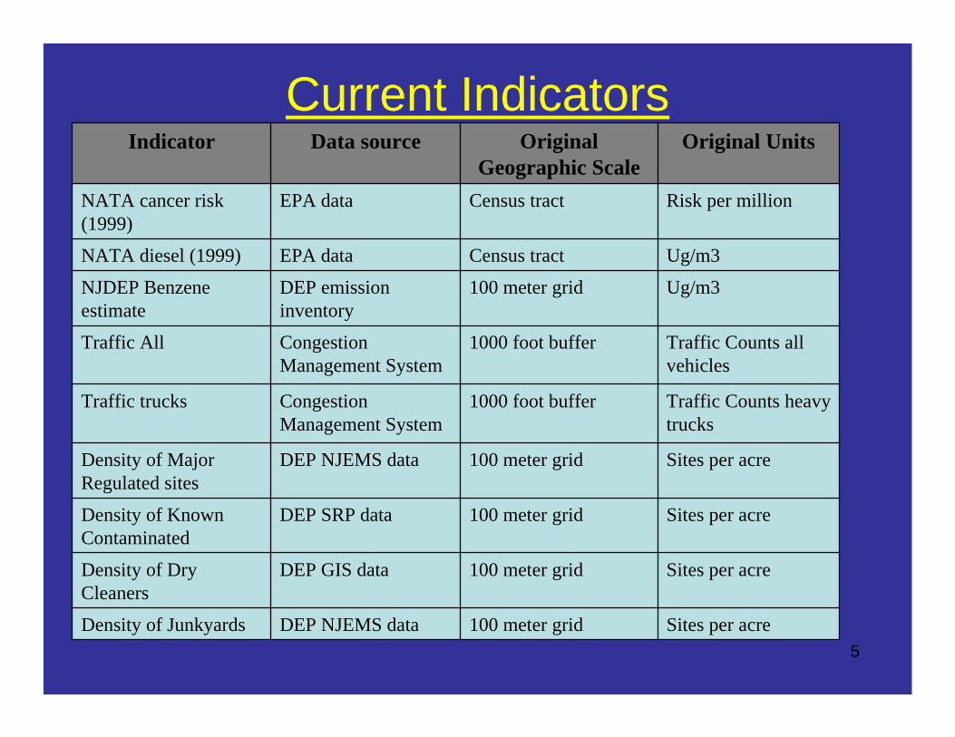
Current Indicators
Sites per acre100 meter gridDEP NJEMS dataDensity of Junkyards
Sites per acre100 meter gridDEP GIS dataDensity of Dry Cleaners
Sites per acre100 meter gridDEP SRP dataDensity of Known Contaminated
Sites per acre100 meter gridDEP NJEMS dataDensity of Major Regulated sites
Traffic Counts heavy trucks
1000 foot bufferCongestion Management System
Traffic trucks
Traffic Counts all vehicles
1000 foot bufferCongestion Management System
Traffic All
Ug/m3100 meter gridDEP emission inventory
NJDEP Benzene estimate
Ug/m3Census tractEPA dataNATA diesel (1999)
Risk per millionCensus tractEPA dataNATA cancer risk (1999)
Original UnitsOriginal Geographic Scale
Data sourceIndicator

6
Indicators from NJ DHSS now Public

7
Options to quantify indicators
• Matrix approach (NEJAC)• Weighting (Faber)
• Scaled Composite Score (EJ SEAT)
• Percentile/quartile distribution• Z-score methodology (Hynes & Lopez)
– Z score = (value-mean)/standard deviation– Normalizes the data to a mean = 0 and standard deviation = 1
Type of Hazardous Facility or Site
Points for Rating Severity of Each Facility or Site
EPA National Priority List Site 25DEP TIER 1A Site 10 10DEP TIER 1B 8 8DEP TIER 1D 8DEP TIER 1C 6 6DEP TIER 2 4 4DEP Other Sites 1 1

8
Options for Geographic Analysis• Use Administrative/political boundaries
– Ex. Faber used municipalities or counties– Count per square mile
• Grided spatial analysis (Rasters in GIS)– Create grid for each indicator at small geographic scale– Use consistent statewide grid

9
Methods to Calculate and Combine Indicators
• Calculate z-score for each indicator in each grid– Statewide grid just over 2 million grids
• Eliminate outliers, z-score >3 are assigned a score of 3– This impacts less than 0.5% of grids
• Two options used to combine indicators:
– Option 1: Sum all z-scores in each grid • Maximum score of 27 (9 indicators) * (3 max z score)• Quantifies how all indicators impact one area• One or two high indicators can drive results
– Option 2: Count each grid with a z score greater than 1• Maximum score of 9 (9 indicators) * (1 count if z >1 )• Focuses more on higher scores• Highlights areas with multiple high indicators

10
Presentation of Results• Some caveats on presentation of results……
• To display data, particularly on maps, we need to make certain decisions on methods and parameters (cut points)
• For example…– How many cut points or groups to present– Equal Interval method: (separate by range in data, highlights changes in
the extremes) – Quantile method: (separate by number of records, highlights changes in
the middle values of the distribution)– Natural break method: (a balance between equal interval and quantile)
• Decisions made to present results may NOT be the policy decisions needed to identify communities of concern

11
Results Option 1: Summation of all scores
•Two cut points
•Above zero and below zero
LegendCounties
Grid Impact Summation Method<VALUE>
-6.1 - 00.1 -24.9
±0 210,000 420,000105,000 Feet
For Illustration Purposes Only

12
Results Option 1: Summation of all scores
•10 Cut points
•Natural breaks (Jenks)
LegendCounties
Grid Impact Summation Method<VALUE>
-6.1 - -2.1-2 - -0.7-0.6 - 0.91 - 2.82.9 - 4.95 - 7.67.7 - 10.510.6 - 13.613.7 - 1717.1 - 24.9
±0 210,000 420,000105,000 Feet
For Illustration Purposes Only

13
Results Option 2: Count of all scores >1
• two cut points
• No indicators above 1
• 1 – 9 Indicators above 1
LegendCounties
Grid Impact Count MethodVALUE
01 - 9±
0 210,000 420,000105,000 Feet
For Illustration Purposes Only

14
Results Option 2: Count of all scores >1
LegendCounties
Grid Impact Count MethodVALUE
0123456789±
0 210,000 420,000105,000 Feet
For Illustration Purposes Only

15
Estimating impacts in larger areas• Grid-level data provides useful information at local level and ability
to “aggregate up” to larger levels
• Impact estimates at larger areas useful to link to other information, such as socio/economic information
• Scale up to “block group” estimates– Smallest area with Census data on income/poverty– There are ~ 6,500 block groups in New Jersey– Average area of ~ 800 acres– Average population of ~ 1,300
• Methods – Zonal Statistics tool in Spatial Analyst– Determine Maximum grid in block group – Weighted Average of all grids in block group

16
Estimating impacts in larger areas
• Calculated for both Summation and Count methods• Final Block Group data has four impact scores:
Summation Method Count Method(1) Max Grid (3) Max Grid
(2) Mean of all grids (4) Mean of all grids

17
NJ Census Data for Socio/Economic Status Percent Minority
• Several States identify communities based on minority and incomecriteria– Pennsylvania, New York, Massachusetts, Indiana, Minnesota
• Northern New Jersey Metropolitan Transportation Planning Authority also identifies communities based on race and income
• DEP has not identified areas base on race and income
• Other screening methods add race, income and other “vulnerability”indictors as part of combined scoring
• DEP is currently using race and income data as separate independent indicators to understand relationship with impact scores

18
NJ Census Data for Percent Minority
• 10 cut points
• Natural breaks
LegendCounties
Block Groups Percent Minority
0.00 - 0.070.08 - 0.120.13 - 0.190.20 - 0.280.29 - 0.380.39 - 0.500.51 - 0.630.64 - 0.780.79 - 0.900.91 - 1.00
±0 210,000 420,000105,000 Feet
For Illustration Purposes Only

19
Relationship between Cumulative Impact and Social/Economic Indicators
Figure 1: Relationship Between Cumulative Impact and Percent Minority
00.5
11.5
22.5
33.5
44.5
5
<0.10 0.10 to0.20
0.20 to0.30
0.30 to0.40
0.40 to0.50
0.50 to0.60
0.60 to0.70
0.70 to0.80
0.80 to0.90
>0.90
Percent Minority
Mea
n Co
unt >
1
• Grouped all block groups based on percent minority and poverty
• Calculated average cumulative impact score for combined groups
• Cumulative impact scores increase steadily with increasing percent minority and poverty
Figure 2: Relationship Between Cumulative Impact and Poverty
0.000.501.001.502.002.503.003.504.004.505.00
< 2.5 2.5 to5
5 to7.5
7.5 to10
10 to12.5
12.5to 15
15 to17.5
17.5to 20
20 to25
>25
Percent Poverty
Mea
n Cou
nt >
1

20
Next Steps on Finalizing Methods
• Updates/improvements to existing indicators– NATA 2002 results– KCS list for 2009
• Potential new indicators– Drinking Water
• Community water systems• Private Well Testing Act
– Ground Water and Soil data– Air quality data for Ozone and PM2.5
• Hierarchical Bayesian data combining monitoring and modeling (CMAQ)