A preliminary investigation of the yellowfin tuna (Thunnus albacares) population in the Atlantic Ocean using the integrated stock assessment model, MULTIFAN-CL

By

P. de Bruyn*, V. Restrepo† and G. Scott†

*AZTI Tecnalia Herrera Kaia, Portualde z/g 20100 Pasaia Basque Country, Spain † NOAA Fisheries Southeast Fisheries Science Center 75 Virginia Beach Drive, Miami, Florida, USA

ABSTRACT

The ICCAT tropical tuna working group proposed that a stock assessment of yellowfin tuna (Thunnus albacares) in the Atlantic Ocean should be attempted using the fully integrated stock assessment model MULTIFAN-CL. Two model variations were attempted. The base case model assumed a single recruitment event per year, with a variation model assuming a recruitment event every three months. Unfortunately, tagging data were not included in these models as several inconsistencies were found in the tagging database. The outputs from both the base case and quarterly recruitment models appear to be overly optimistic. For the base case model, current Biomass was estimated to be below BMSY, however current F was far below FMSY. For the quarterly recruitment model, both reference points were well within their estimated MSY values. These findings are inconsistent with the output of previous stock assessments on this species in the Atlantic region. The base case model estimated higher levels of both current as well as initial biomass than the quarterly recruitment model. This assessment should be viewed as part of an ongoing process, as the addition of tagging data may well result in a more realistic assessment of the yellowfin tuna stocks in the region.

1 Introduction Yellowfin tuna (Thunnus albacares) is a cosmopolitan species distributed mainly in tropical and subtropical oceanic waters. In the tropical Atlantic, yellowfin tuna are caught in the entire ocean, between 45ºN and 40ºS, by surface gears (purse seine, baitboat and handline) and by longline fisheries. In the East Atlantic, baitboat fisheries operate along the African coast and the various archipelagos in the Atlantic (Azores, Madeira, Canary Islands and Cape Verde) and have been operating since the early 1950s. The East Atlantic purse seine fisheries began in 1963 and developed rapidly in the mid-1970s. They initially operated in coastal areas and gradually extended to the high seas. Since the early 1990s, several purse seine fleets (France, Spain, Ghana and NEI) have operated fisheries using objects. In the West Atlantic, Venezuelan and Brazilian baitboats have been targeting yellowfin tuna since the mid-1960s. The purse seine fisheries, which were sporadic between 1970 and 1980, have operated in coastal areas since 1980 along the north coast of Venezuela and in the south of Brazil, although yellowfin tuna are not targeted by these

SCRS/2008/190

fleets. Longline fisheries capturing yellowfin tuna are found throughout the Atlantic. The longline fishery began at the end of the 1950s, with significant catches being taken by the early 1960s. Since then the catches have gradually decreased. In the Gulf of Mexico, both U.S. and Mexican longline vessels target yellowfin while Venezuelan vessels appear to target yellowfin seasonally. In contrast, Japanese and Chinese Taipei vessels began, in the early 1980s, to shift targeting away from albacore and yellowfin toward bigeye tuna through the use of deep longline. Following a recommendation made by the International Commission for the Conservation of Atlantic Tuna (ICCAT) Tropical Species Group an assessment of the yellowfin tuna stocks was initiated at a Tropical Tuna Species group meeting held in Florianopolis, Brazil in July 2008. This initiative was proposed, as a declining trend of some fishery indicators such as total catch, standardised CPUE, and average weight had been noted in recent years. The working group also recommended that in addition to conventional stock assessment techniques such as Production Modelling, an integrated stock assessment model, namely MULTIFAN-CL (MFCL; Fournier et al, 1998) be initiated for this stock. This paper provides preliminary results for the MFCL model applied to the yellowfin tuna stocks in the Atlantic Ocean. This is by no means a definitive stock assessment, as fully integrated models require significant time to fine tune and optimise in order to obtain realistic model outputs. Instead, this study hopes to provide a basis for further investigation and discussion.

2 Model description and data input MFCL is a computer program that implements a statistical, size-based, age-structured, and spatial-structured model for use in fisheries stock assessment. A comprehensive description of the model is provided in Kleiber et al. (2003). It is used routinely for tuna stock assessments by the Oceanic Fisheries Programme (OFP) of the Secretariat of the Pacific Community (SPC) in the western and central Pacific Ocean (WCPO) while both the Indian Ocean Tuna Commission (IOTC) and ICCAT are proposing the use of this model in regional stock assessments. The model is fit to time series of catch and size composition data from either one or many fishing fleets. Size composition data may be in the form of either length or weight-frequency data, or both. The model may also be fit simultaneously to tagging data, if available. Other information is provided to the model in the form of fishing effort data and “prior” information on estimates of various biological and fisheries parameters and their variability (Hampton 2002). The data used in the yellowfin tuna assessment consist of catch, effort and length-frequency data for the fisheries defined in Table 1. The use of tag release-recapture data was intended, however, the format of this data as well as problems in the ICCAT tagging database resulted in this data being excluded from this assessment. The details of the utilised data and their stratification are described below. 2.1 Spatial Stratification Initially, it was intended that the fisheries be separated into two regions in the Atlantic Ocean, namely the Eastern (East of 30o W) and Western (West of 30o W) regions. Due to the fact that the tagging data was not utilised and hence movement could not be quantified, all the fisheries were grouped into a single region for this assessment. 2.2 Temporal Stratification It was proposed that the working group only utilise data subsequent to 1965. The availability of historical data prior to 1965 enabled the time series of catch and effort data, as well as size frequency data to extend back further than was previously anticipated.

2.3 Fisheries definitions MFCL requires the definition of “fisheries” that consist of relatively homogeneous fishing units. Ideally, the fisheries so defined will have selectivity and catchability characteristics that do not vary greatly over time (although in the case of catchability, some allowance can be made for time-series variation). For most pelagic fisheries assessments, fisheries defined according to gear type, fishing method and region will usually suffice. In total, 18 separate fisheries where defined (Table 1). 2.4 Catch and Effort data Catch and effort data were compiled by fishery. Quarterly effort data by fishery were estimated from the ICCAT Task II c/f data applying Generalized Linear Models controlling for Fleet, Gear Type, and Effort Type within each fishery definition recorded in the Task II c/f database. The 2008 ICCAT yellowfin and skipjack tuna stock assessment meeting report documents the procedures used to generate the time-series CPUE, which was then divided into the fishery specific catch information to estimate effort patterns for MFCL. In all cases, where detailed, standardized CPUE was available from National Scientists or based on work conducted by the Group at the assessment meeting, those CPUE patterns were used to compute quarterly effort patterns for use in MFCL. 2.5 Length Frequency data Size frequency data held in the Task II data set were organized by MFCL fishery definition and quarter for yellowfin tuna. A criterion of at least 50 size observations per fishery/quarter was used to filter the data for use. The size frequency data were compiled into 86, 2 cm length classes (20-22 cm to 188 to 190 cm). Size frequency data were few for the initial years of the model due to a lack of sampling during this time. 3 Structural Assumptions of the model The following structural assumptions were included in the current yellowfin tuna stock assessment model runs. The mathematical specification of structural assumptions is given in Hampton and Fournier (2001). 3.1 Observation models for the data In this model, there are two data components that contribute to the log-likelihood function - the total catch data and the length-frequency data. The observed total catch data are assumed to be unbiased and relatively precise. The probability distributions for the length-frequency proportions are assumed to be approximated by robust normal distributions, with the variance determined by the effective sample size and the observed length-frequency proportion. Due to the vast differences in sample sizes between fisheries, the size frequency data was rescaled to reduce all samples to a maximum of 1000. This was done in order to prevent samples that were raised to the total catch numbers from biasing the length frequencies. 3.2 Recruitment In the base case model, the number of recruitment events was limited to one per year. A variation in the model allowed for quarterly recruitment effectively implying that recruitment is continuous throughout the year. Recruitment was assumed to follow a weak Beverton and Holt stock-recruitment relationship (SRR). The SRR was incorporated mainly so that a yield analysis could be undertaken for stock assessment purposes. A relatively weak penalty for deviation from the SRR was applied so that it would not have a large effect on the recruitment and other model estimates. Fisheries data are usually uninformative about SRR parameters. It was thus necessary to

constrain the parameterisation in order to maintain stable model behaviour. A beta-distributed prior on the “steepness” (S) of the SRR was included, with S defined as the ratio of the equilibrium recruitment produced by 20% of the equilibrium unexploited spawning biomass to that produced by the equilibrium unexploited spawning biomass (Francis 1992; Maunder and Watters 2001). The prior was specified by mode = 0.9 and SD = 0.04 (a = 46, b = 6). In other words, a reduction in equilibrium recruitment when the equilibrium spawning biomass is reduced to 20% of its unexploited level would be fairly small (a decline of 10%). This assumption was based on the stock assessment of yellowfin tuna carried out in the central Pacific Ocean (Hampton 2002). 3.3 Age and Growth For MFCL, it is necessary to assume the number of significant age-classes in the exploited population, with the last age-class being defined as a plus group. For the results presented here, 40 quarterly age-classes have been assumed. A standard Von Bertalanffy growth curve was assumed. The model was used to estimate both K and L infinity from the data, although informative priors of 0.3 and 180 cm respectively were used (Wild 1994) as these values were also estimated using length frequency techniques. The value for K was divided by four in the quarterly model to account for the increased number of recruitments as recommended by Kleiber et al. (2003). Previous analyses assuming a standard von Bertalanffy growth pattern indicated that there was substantial departure from the model (Gascuel et al. 1992) therefore in this case, growth was modelled by allowing the mean lengths of the first eight quarterly age-classes to be independent parameters. 3.4 Selectivity Selectivity is fishery-specific and was assumed to be time-invariant. Longline fisheries were assumed to have non-decreasing selectivity with age. The coefficients for the last fifteen quarterly age-classes, for which the mean lengths are very similar, are constrained to be equal for all fisheries. 3.5 Catchability and Effort variability A time series of catchability was estimated for each fishery, and random walk steps were taken every two years. The seasonal component of catchability was also estimated. Effort deviations, constrained by prior distributions of zero mean, were used to model the random variation in the effort – fishing mortality relationship. Prior variance levels were set to a moderate level for all fisheries (corresponding to a CV of about 0.32) 3.6 Initial Population The population age structure in the initial time period is determined as a function of the average total mortality during the first 20 quarters. This assumption avoids having to treat the initial age structure as independent parameters in the model. 3.7 Natural Mortality Natural mortality rates were estimated for each age. They were considered constant over time.

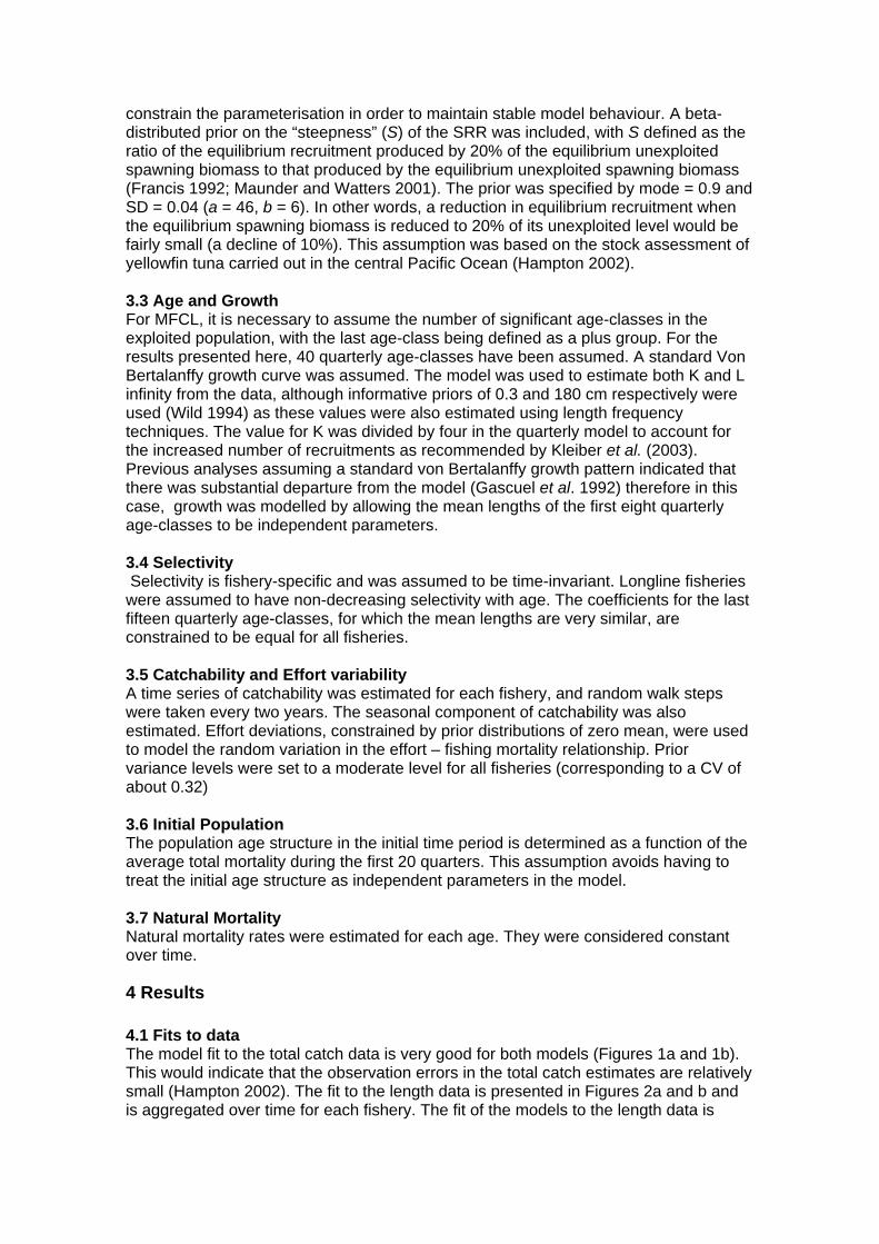
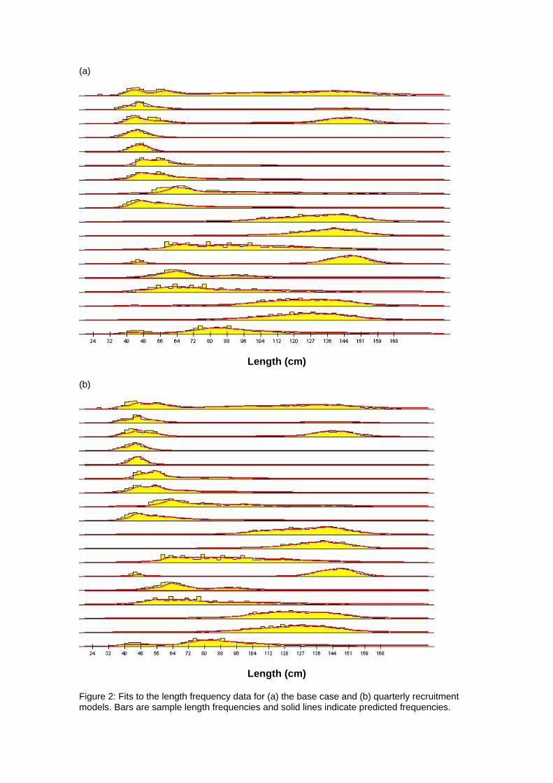
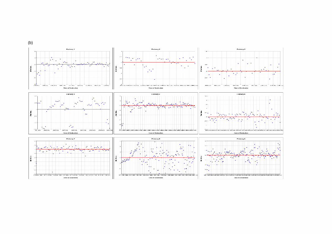
4 Results 4.1 Fits to data The model fit to the total catch data is very good for both models (Figures 1a and 1b). This would indicate that the observation errors in the total catch estimates are relatively small (Hampton 2002). The fit to the length data is presented in Figures 2a and b and is aggregated over time for each fishery. The fit of the models to the length data is

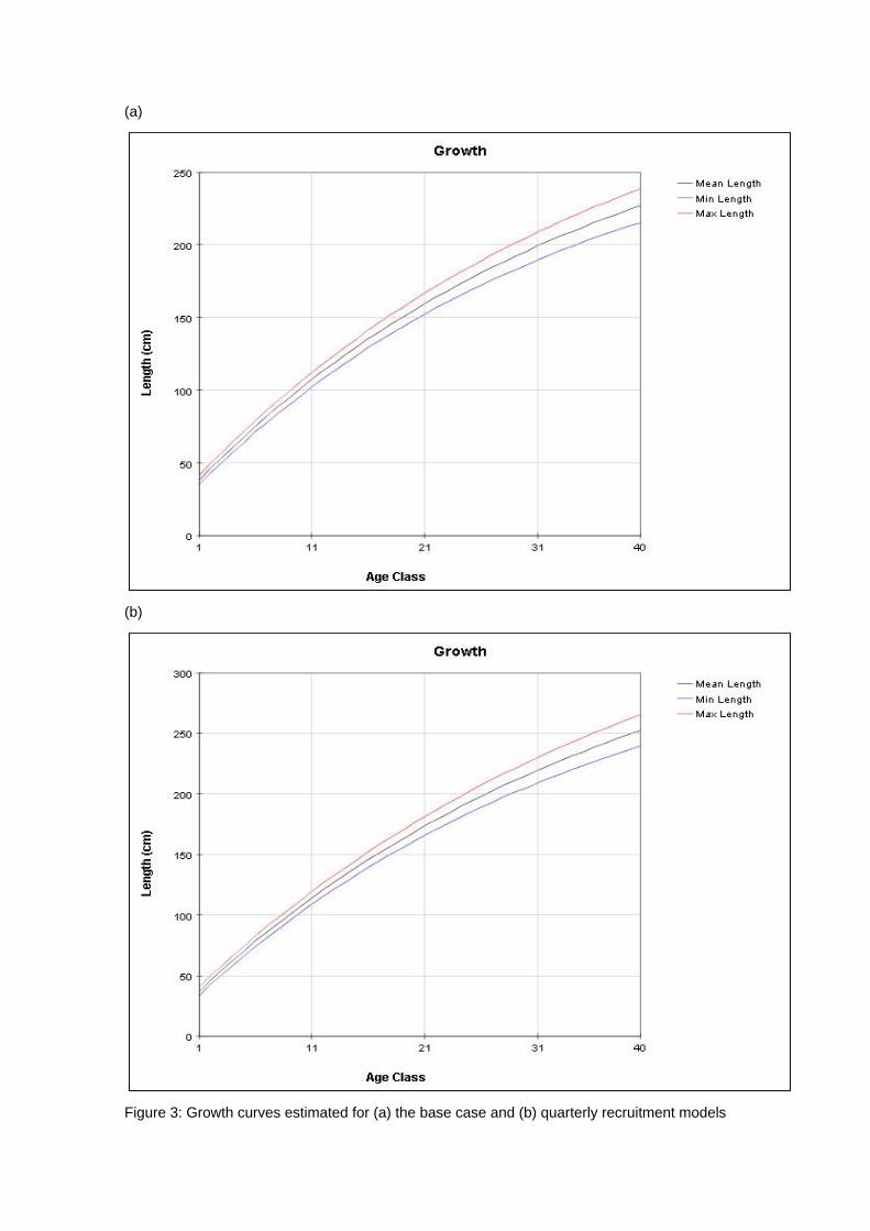
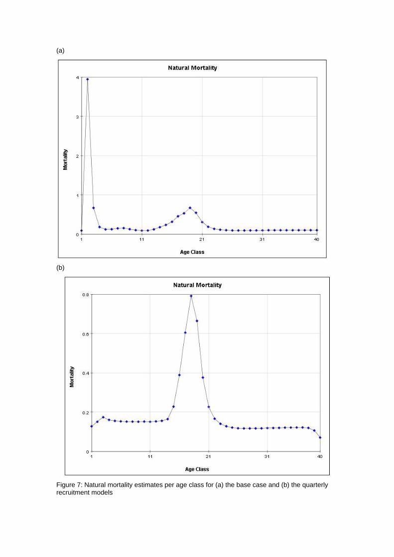
generally quite good, although there are deviations, particularly for the smaller sized fish. 4.2 Age and Growth The models were able to detect a coherent growth signal in the size data. The estimated growth curves for each model are shown in Figures 3a and b. The model fitted a fairly standard von Bertalanffy growth and the deviation of this pattern in the first 8 quarterly age classes was not clearly apparent. Neither model appeared to reach a clear asymptote, and so reliable estimates of L infinity were impossible to obtain. 4.3 Selectivity Estimated selectivity coefficients are presented in Figures 4a and b. In both models, the purse seine fisheries selectivities are different for free and FAD sets (modelled since 1990). With the FAD sets showing a non-decreasing selectivity with age. Selectivites for the free school sets are similar to those for all purse seine sets between 1980 and 1990, while purse seine sets prior to 1980 display similar selectivites to the FAD sets. Longline selectivity coefficients were all similar between fisheries, as were the baitboat selectivities. All showed a non-decreasing selectivity with age with the longline fisheries increasing at an earlier age than the baitboat fisheries. For the quarterly recruitment model, peaks in selectivity were estimated for small sizes. The reasons for these peaks are not immediately apparent as they are not clearly supported by the length frequency data. 4.4 Catchability Time series estimates of catchability are presented in Figures 5a and b. Changes in trends over time are evident for several fisheries. In general , the purse seine fisheries displayed increases in catchability over time, although this trend was more apparent in the base case model. The majority of fisheries also displayed significant fluctuations in seasonal catchability. The overall consistency of the model with the observed effort data can be examined in plots of effort deviations against time for each fishery. If the model is coherent with the effort data, an even scatter of effort deviations about zero would be expected although some outliers would also be expected. If there was an obvious trend in the effort deviations with time, this may indicate that a trend in catchability had occurred and that this had not been sufficiently captured by the model (Hampton 2002). For the majority of fisheries there are no obvious trends in the effort deviations (Figures 6a and b). This would indicate that the model has extracted most of the information present in the data regarding catchability variation. 4.5 Natural Mortality The model calculated natural mortality shows considerable variation with age (Figures 7a and b). For the base case model, the natural mortality decreases rapidly during the first yearly age group, remains fairly constant until the beginning of the fourth year, at which stages it increases again until the end of the sixth year after which it remains constant. This overall shape is similar to that found for the central Pacific Ocean, although the overall M values in this study are far higher and the mortality estimates in that study were higher for mature individuals (the second peak) than the initial year class (Hampton 2002). For the quarterly recruitment model, the natural mortality is generally fairly consistent with the exception of a large peak during the fourth and fifth year classes. The overall values of natural mortality are, however, more similar to those found in the central Pacific study. 4.6 Recruitment Model estimated recruitment appeared to be very high (Figures 8a and b), ranging between 15 billion and 5 billion individuals annualy for the base case model. This clearly is an over-estimation of recruitment, and needs to be addressed in future model

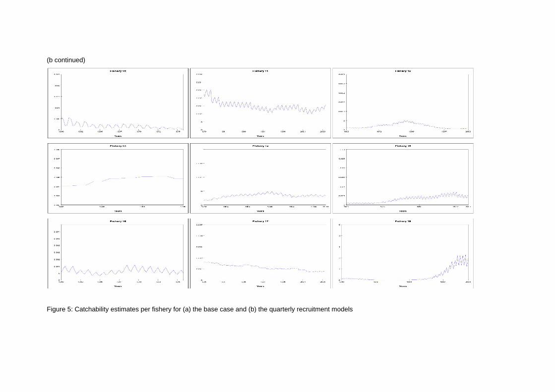
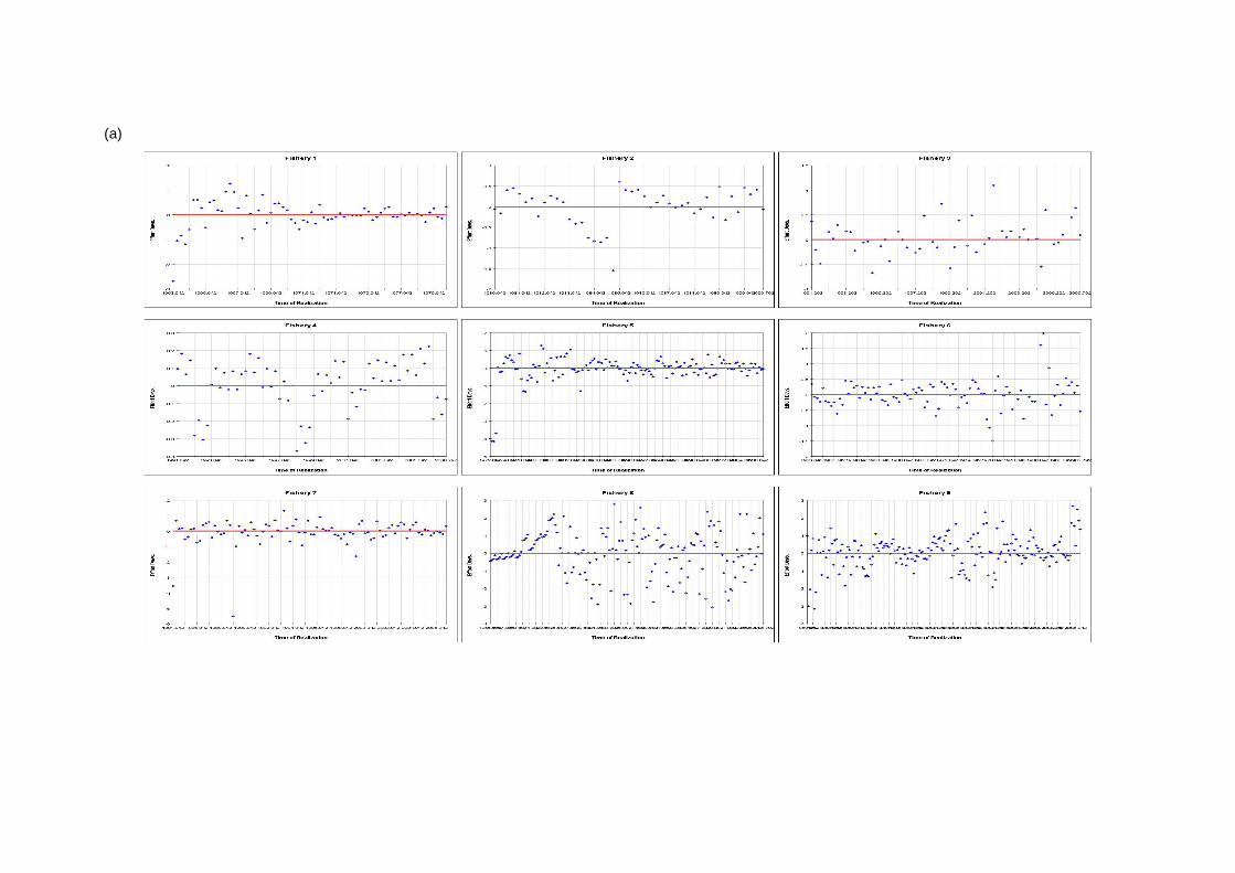
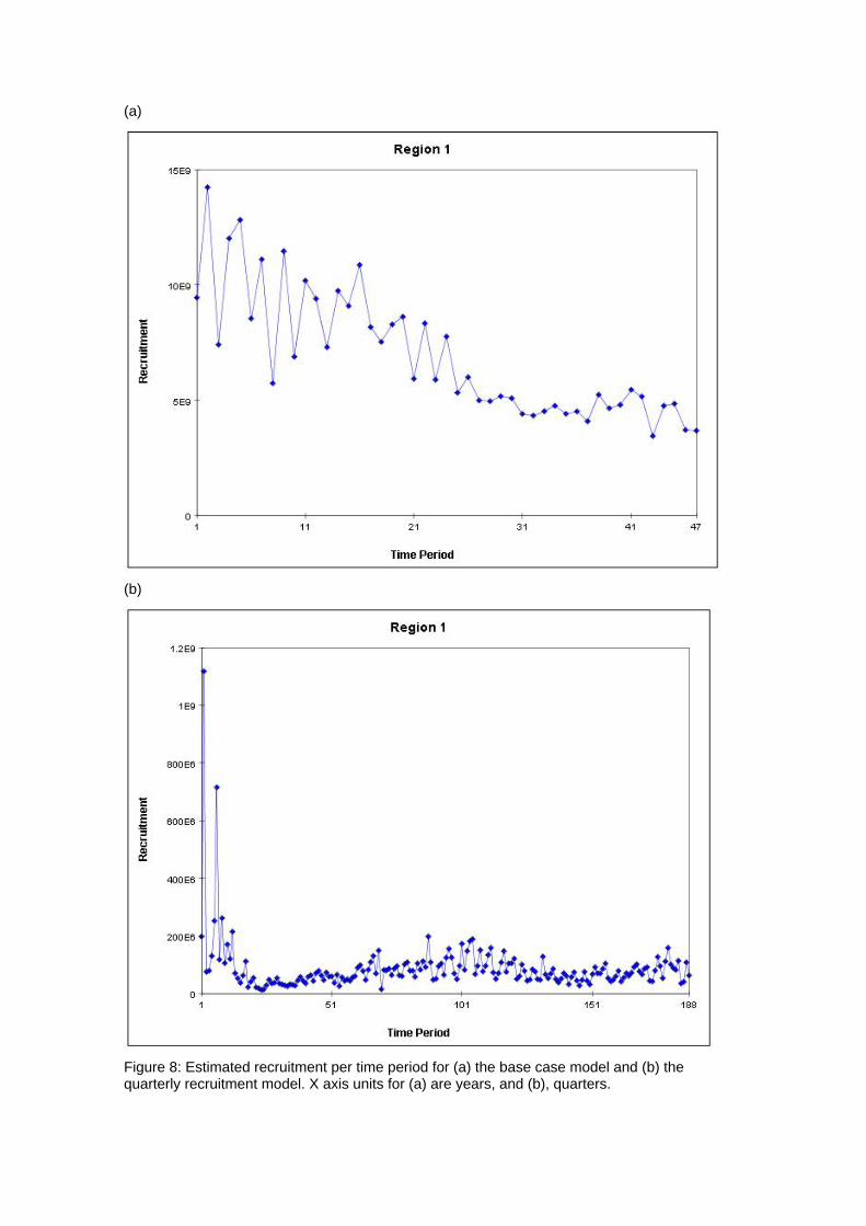
runs. This over-estimation has led to overly optimistic stock indicators which are discussed below. What is possibly more informative is the trend in recruitment. Although recruitment fluctuated markedly in the initial years of the model, there has been a clear negative tend in recruitment over time. The last few quarters displayed the lowest estimates of recruitment for the entire series. For the quarterly recruitment model, recruitment levels at the beginning of the time series were very high, but have stabilised over time although there were significant seasonal fluctuations estimated by this model. The level of recruitment was significantly lower than the base case model, usually less than 800 million individuals per year. 4.7 Biomass Time series of total and adult biomass are shown in Figures 9a and b. For the base case model, total biomass as well as adult biomass has decreased over time. This is reflective of the overall decreasing trend in recruitment and increasing catch levels. This decrease was most notable in the 1980s, but has continued until recent times. Despite this decrease total biomass remains fairly high due to the estimated high levels of recruitment. In the quarterly recruitment model, biomass appeared to increase initially, dropping off rapidly after mid way through the 1960s. Since that time, both total and adult biomass has remained fairly constant with a smaller peak approximately 40 years into the time series (1990s) before decreasing again. Again, this mirrors trends in the predicted recruitment. 4.8 Fishing Mortality Average fishing mortality rates are shown in Figures 10a and b. For the base case model, F values have been steadily increasing over time with a small decrease in the early 1980s the early 2000s. This trend is generally consistent with the overall catch numbers reported for the Atlantic region. For the quarterly recruitment model, the pattern is slightly different, with F values increasing rapidly until the early 1980s at which stage they are estimated to have reduced significantly with a gradual increase until the early 2000s. The major difference between the two model estimations is relative size of the two F peaks, with the quarterly recruitment model estimating the highest F values in the late 1970s as opposed to the early 2000s in the base case model. 4.9 Yield Analysis The yield analysis conducted here incorporated the stock-recruitment relationship (Figures 11a and b) into the equilibrium biomass and yield estimates. The steepness for both models was estimated to be 0.901, which is almost identical to the prior mode of 0.9. As far as both the current analyses are concerned, there appears to be no strong relationship between the spawning stock and recruitment. Management quantities estimated in the model are given in Table 2. Equilibrium total and adult biomass at unexploited levels are 26,070,000 t and 2,795 000 t, respectively for the base case model and 6,329,000 t and 1,905,000 t respectively for the quarterly recruitment model. The current fishing level is far below the MSY level predicted from either model (Figures 11a and b). The base case model does, however, estimate that current total biomass is still lower than BMSY but F is lower than FMSY (Figures 12a and b). Both models thus predicted that the stock is not being over-exploited. Again, this is almost certainly over-optimistic, and future model runs may very well indicate that this is not the case.

5 Discussion This paper has presented the results from two preliminary attempts to model the dynamics of the yellowfin tuna stock in the Atlantic Ocean. At this stage, it is clear that

further work is needed to refine these models, as although they provide some useful insights into the stock, they are not yet suitable for management advice. Compared with other stock assessment models presented at ICCAT working groups on tropical tuna stock assessments in recent years (Anon 2004), the outputs and reference points generated by these models are extremely optimistic. These models should thus be viewed as a step towards obtaining a fully integrated stock assessment model for the Atlantic Ocean yellowfin tuna stocks. Of primary importance for these models, is the future inclusion of tagging data. This will allow spatial stratification of the model, and will provide a more realistic assessment of the tuna stock. Further refinement of the input parameters and prior distributions, to optimise the model fit, are also of importance. It is clear, however, that these models have great potential for the assessment of tropical tuna stocks. Priority will be given to resolve these issues and work on these models is ongoing. References Anon 2004. 2003 ICCAT Atlantic yellowfin tuna stock assessment session. Col. Vol.

Sci. Pap. ICCAT, 56(2): 443-527. Fournier, D.A., Hampton, J., and Sibert, J.R. 1998. MULTIFAN-CL: a length-based,

age-structured model for fisheries stock assessment, with application to South Pacific albacore, Thunnus alalunga. Can. J. Fish. Aquat. Sci. 55: 2105 - 2116.

Francis, R.I.C.C. 1992. Use of risk analysis to assess fishery management strategies: a

case study using orange roughy (Hoplostethus atlanticus) on the Chatham Rise, New Zealand. Can. J. Fish. Aquat. Sci. 49: 922 - 930.

Gascuel, D., Fonteneau, A and Capisano, C. 1992. Modélisation d’une croissance en

deux stances chez l’albacore (Thunnus albacares) de l’Atlantique est. Aquat. Living Resour. 5(2): 155-172.

Hampton, J. 2002. Stock assessment of yellowfin tuna in the western and central

Pacific Ocean. 15th SCTB, Hawaii, 22-27th July 2002, Oceanic Fisheries Programme, Secretariat of the Pacific Community, Noumea, New Caledonia. Working Paper YFT-1:39 pp

Hampton, J., and Fournier, D.A. 2001. A spatially-disaggregated, length-based, age-

structured population model of yellowfin tuna (Thunnus albacares) in the western and central Pacific Ocean. Mar. Freshw. Res. 52:937 - 963.

Kleiber, P., Hampton,J. and Fournier, D.A. 2003. MULTIFAN-CL Users’ Guide.

http://www.multifancl.org/userguide.pdf. Maunder, M.N., and Watters, G.M. 2001. A-SCALA: An age-structured statistical catch-

at-length analysis for assessing tuna stocks in the eastern Pacific Ocean. Background Paper A24, 2nd meeting of the Scientific Working Group, Inter-American Tropical Tuna Commission, 30 April - 4 May 2001, La Jolla, California.

Wild, A., 1994. A review of the biology and fisheries for Yellowfin Tuna, Thunnus

albacares, in the eastern Pacific Ocean. p. 52-107 In R.S. Shomura, J. Majkowski and S. Langi (eds.), Interactions of Pacific tuna fisheries. FAO Fisheries Technical Paper 336(2), 439 p.

Table 1. Fishery definitions proposed for the 2008 yellowfin tuna stock assessment using MULTIFAN-CL. Fishery Gear Nation Years

# 1 PS EC France, EC Spain, Others 1960-1979 # 2 PS EC France, EC Spain, Others 1980-1990 # 3 PS EC France, EC Spain, Others, free

schools Qtr 2-4 1991 - 2006

# 4 PS EC France, EC Spain, Others, FADS 1991 - 2006 # 5 PS&BB Ghana (1973 - 2005) 1960 - 2006 # 6 BB EC France, EC Spain (Dakar based),

Senegal 1965 - 1983

# 7 BB EC France, EC Spain (Dakar based), Senegal

1984 - 2006

# 8 BB Azores, Madeira, Canaries 1960 - 2005 # 9 BB Others 1960 - 2006 # 10 LL ALL 1960 - 1975 # 11 LL ALL 1976 - 2006 # 12 OTH Others 1960 - 2006 # 13 PS EC France, EC Spain, Others, free

schools Qtr 1 1991 - 2006

# 14 BB Brazil 1960 - 2006 # 15 PS&BB Venezuela 1960 - 2006 # 16 LL All 1960 - 1975 # 17 LL All 1976 - 2006 # 18 Others Others 1960 - 2006

Table 2. Estimates of management reference points Reference point Base case Quarterly recruitment model MSY 433,300 t 201,800 t Biomass at MSY 17,800,000 t 2,776,000 t Spawning Biomass at MSY 343,100t 403,500 t Initial Biomass 26,070,000 t 6,329,000 t Initial Spawning Biomass 2,795 000 t 1,905,000 t Fcurrent/FMSY 0.27 0.04 Bcurrent/BMSY 0.89 2.62

(a)

Tota

l num

ber o

f fis

h ca

ught

Year

(a continued)

Tota

l num

ber o

f fis

h ca

ught

Year

(b)

Tota

l num

ber o

f fis

h ca

ught

Year

(b continued)

Figure 1: Observed and predicted total catch numbers by fishery and by quarter for (a) the base case and (b) quarterly recruitment MFCL models

Year

Tota

l num

ber o

f fis

h ca

ught

(a)

Length (cm)

(b)

Length (cm)

Figure 2: Fits to the length frequency data for (a) the base case and (b) quarterly recruitment models. Bars are sample length frequencies and solid lines indicate predicted frequencies.

(b)

Figure 3: Growth curves estimated for (a) the base case and (b) quarterly recruitment models

(a)

(a)

(a continued)

(b)

(b continued)

Figure 4: Selectivity estimates per fishery for (a) the base case and (b) the quarterly recruitment models

(a)

(a continued)

(b)

(b continued)

Figure 5: Catchability estimates per fishery for (a) the base case and (b) the quarterly recruitment models

(a)

(a continued)

(b)

Figure 6: Effort deviation estimates per fishery for (a) the base case and (b) the quarterly recruitment models

(b continued)

(a)

(b)

Figure 7: Natural mortality estimates per age class for (a) the base case and (b) the quarterly recruitment models

(b)

Figure 8: Estimated recruitment per time period for (a) the base case model and (b) the quarterly recruitment model. X axis units for (a) are years, and (b), quarters.

(a)

Figure 9: Estimated total and adult biomass trends over time for (a) the base case and (b) the quarterly recruitment models. In both cases, the time period units are years.

(a)

(b)

(a)

0

0,5

1

1,5

2

2,5

3

3,5

4

1950 1960 1970 1980 1990 2000 2010

Year

F

(b)

0

0,5

1

1,5

2

2,5

3

3,5

4

4,5

1950 1960 1970 1980 1990 2000 2010Year

F

Figure 10: Fishing mortality rate time series for (a) the base case and (b) the quarterly recruitment models

(a)

(b)

Figure 11:Recruitment estimates and the fitted Beverton and Holt stock-recruitment relationship

(SRR) for (a) the base case and (b) the quarterly recruitment models incorporating a prior on steepness of 0.9.