a practical manual for vissim com programming in matlab · as well. the principle of com...

If you find this manual useful, please, cite this paper: https://doi.org/10.3311/pp.ci.2012-1.05

Budapest University of Technology and Economics

Dept. for Control of Transportation and Vehicle Systems

www.traffic.bme.hu

2018

A practical manual for Vissim COM

programming in Matlab 3rd edition for Vissim version 9 and 10

Tamás Tettamanti, Márton Tamás Horváth

https://doi.org/10.3311/pp.ci.2012-1.05

http://www.traffic.bme.hu/


1

1. Vissim traffic simulation via COM interface programming

1.1. The purpose of Vissim-COM programming

Vissim is a microscopic road traffic simulator based on the individual behavior of vehicles.

The goal of the microscopic modeling approach is the accurate description of the traffic

dynamics. Thus, the simulated traffic network may be analyzed in detail. The simulator uses

the so-called psycho-physical driver behavior model developed originally by Wiedemann

(1974). Vissim is widely used for diverse problems by traffic engineers in practice as well as

by researchers for developments related to road traffic. Vissim offers a user friendly graphical

interface (GUI) through of which one can design the geometry of any type of road networks

and set up simulations in a simple way. However, for several problems the GUI is not

satisfying. This is the case, for example, when the user aims to access and manipulate Vissim

objects during the simulation dynamically. For this end, an additional interface is offered

based on the COM which is a technology to enable interprocess communication between

software (Box, 1998). The Vissim COM interface defines a hierarchical model in which the

functions and parameters of the simulator originally provided by the GUI can be manipulated

by programming. It can be programmed in any type of languages which is able to handle

COM objects (e.g. C++, Visual Basic, Java, etc.). Through Vissim COM the user is able to

manipulate the attributes of most of the internal objects dynamically.

1.2. The basic steps of Vissim-COM programming

The following steps formulate a general synthesis for the realization of any adaptive control

logic through Vissim-COM interface:

1. One generates the overall traffic network through the Vissim GUI (geometry, signal

heads, detectors, vehicle inputs, etc.).

2. After choosing a programming language which allows COM interface programming,

one creates the COM Client.

3. Programming of the simulation via Vissim COM with specific commands, e.g.

simulation setting (multiple and automated runs),

vehicle behavior,

evaluation during simulation run (online),

traffic-responsive signal control logic.

4. Simulation running form COM program.

To understand the Vissim-COM concept, see the figure below which depicts a part of the

Vissim-COM object model. The Vissim-COM is based on a strict object hierarchy with two

kinds of object types:

collections (array, list): store individual objects, references to the objects; the

collection names in the Vissim-COM object model are always in plural, e.g. ‘Links’.

The interface for this object is the ‘ILinks’ interface. References to the objects can be

accessed via the ‘ILinkCollection’ interface.

containers: store a single object, the objects themselves; the container names are

always in singular, e.g. ‘Link’. The interface for this object is the ‘ILink’ interface.

The objects themselves can be accessed via the ‘ILinkContainer’ interface.



2

‘This distinction between containers and collections is needed because objects are linked to

one another. Adding new objects or deleting objects is only possible in the container.’ (PTV,

2017)

The letter ‘I’ always represents the interface for the object.

The objects are in a hierarchical structure of which the head is the main Vissim object. IVissim

is the interface representing the Vissim object. Only one main object can be defined and all

other objects belong to the main object.

1. The Vissim-COM object hierarchy (PTV, 2017)

The full Vissim-COM object hierarchy model is described in the Online Help of Vissim that

can be accessed via the Vissim GUI. Click on Help\Online Help…\Vissim-COM\Objects. To

access the IVissim interface, representing the Vissim object, click on IVissim (see fig. 2). Under

the Public Properties headline you can see five properties that return object instances. These are

Evaluation, Graphics, Net, Presentation and Simulation. Thus IEvaluation, IGraphics, INet,

IPresentation and ISimulation interfaces, representing the Evaluation, Graphics, Net,

Presentation and Simulation objects, are available.



3

2. Accessing the objects of Vissim (Vissim online help)

To understand the object model, consider the following example, which represents the access

to a given road link:

1. Below the main interface ‘IVissim’ (representing the ‘Vissim’ object, see fig. 1) you

can find the ‘INet’ interface (representing the ‘Net’ object), which compasses all

network functionalities.

2. Collections are situated below object ‘Net’ (of which the interface is ‘INet’).

3. Collection ‘Links’ (of which the interface is ‘ILinkContainer’) contains the references

to the links of the network (previously defined via Vissim GUI). ‘Links’ is a Public

Property of ‘INet’. The Link objects themselves are contained in the Links object for

which ‘ILinkCollection’ is the interface (The same is valid for e.g. ‘Areas’ and

‘IAreaCollection’).

4. To access a given ‘Link’ object, one needs to define ‘Vissim’, ‘Net’, and ‘Links’ objects.

‘ILinkContainer’ (and containers generally) has a Public Property called ‘ItemByKey’

that makes it possible to access the ‘ILink’ interface for a specific Link object

5. After accessing the given ‘Link’, one may apply Vissim-COM methods (e.g.

‘RecalculateSpline’), as well as query or set attributes (e.g. ‘NAME’).

This example is presented now by Visual Basic Script language. This practically shows the

access to Link 10 (after the apostrophe character you can read comments):

Set vis = CreateObject(‘Vissim.Vissim’) 'define Vissim main object

Set vnet = vis.Net 'define Net object

vis.LoadNet(‘D:\Example\test.inpx’) 'Load the traffic network

Set links = vnet.Links 'define Links collection

Set link_10 = links.ItemByKey(10) 'Query Link 10 as an object



4

1.3. How to use Matlab for Vissim-COM programming?

In the following chapters the Vissim-COM programming is introduced by using Matlab Script

language. For this the Vissim-COM interface manual (PTV, 2017) used to provide a detailed

help until Vissim version 5 but since then the official offline help is significantly less detailed.

Instead of that you can use the online help (in the Vissim GUI click on Help\Online Help…)

or the official examples provided for Vissim. Although the examples of this official manual

are basically written in Visual Basic, the document also provides a short help so that we can

transform the scripts into other programming languages (therefore into Matlab environment)

as well. The principle of COM programming is the same written in any language.

One of the main advantages of using Matlab is the simplicity of the Matlab Script language.

Another very important aspect is that Matlab (as a mathematical software package for

practical purposes) has a lot of built-in functions. For example, optimization tasks can be

solved with the help of simple Matlab commands, statistical functions can be called freely or

simple matrix usage can be achieved. With the functions provided by Matlab a lot of time and

energy can be spared compared to other programming languages. Therefore, if you are

programming the Vissim traffic simulator via COM, but you also want to perform special

operations (e.g. optimization), it is highly recommended to choose the Matlab Script as the

basic language for programming Vissim-COM.

Important technical information is that before creating a Vissim-COM program, you must

register the Vissim as a COM-server in your operating system (so that other applications can

access Vissim-COM objects). You can do the registration after the installation of Vissim by

clicking on menu ‘Help/Register COM server’.



5

2. Creating Vissim-COM server in Matlab

User may create a script file (extension ‘.m’) in Matlab with the ‘File/New/Script’ menu or

with the white paper icon located in the toolbar (see figure below).

3. Creating Matlab Script file (extension ‘.m’)

In the Matlab Script code you can write comments after the % sign.

It is useful to start ‘.m’ files with two basic commands:

clear all;

close all;

The first deletes the contents of the Matlab workspace, i.e. the currently used variables and

their values. Delete is very useful to avoid errors, e.g. the remained values of the variables in

the previous executing may cause confusion. The second command closes all of the opened

Matlab windows (e.g. diagrams) in one step.

Creating a new COM server (other name ActiveX) is possible with the use of the Matlab

command ‘actxserver’:

vis=actxserver('VISSIM.vissim.900')

For detailed information about a Matlab command use the Command Window and write the

‘help’ before the command e.g.

help actxserver



6

3. Vissim-COM methods

Object methods created via the Vissim-COM server are also accessible in the Command

Window. The list of the objects can be found in the Vissim-COM Interface Manual (PTV,

2017). We can access the method list of each object if we type the object’s name and the

‘methods’ command with a dot between them into the Command Window:

{Vissim-COM object name}.methods

The method above can only be used if the object written between the curly braces was defined

beforehand. For example take a look at the following figure, which can be used for the object

‘vis’ (main object predefined in the previous chapter), and shows the list of all methods.

4. Getting the method list of the object ‘vis’ in Matlab

From the method list above the ‘invoke’ is shown below as an example.

5. The answer of Matlab Command Window to the ‘invoke’ command of a Vissim-

COM object

As it can be seen, the list shows the available methods with the return value types and

arguments. The ‘variant’ is a variable type which involves several types. ‘void’ means that

the method does not have any return values.



7

Similarly, the methods concerning any other Vissim-COM object can be listed analogously.

Another useful Matlab command is applicable to reveal the properties of an object. This can

be done by ’fields’ command:

{Vissim-COM object name}.fields

6. The answer of Matlab Command Window to the ‘fields’ command of a Vissim-COM

object



8

4. Loading of Vissim network

In case of Vissim-COM programming you must create the simulation network and its

elements on the graphic interface of the Vissim. You will get a project file that has an .inpx

extension, and a ‘Layout’ file with .layx extension. Then, you can infuse them from the COM

program with ‘LoadNet’ and ‘LoadLayout’ methods. While you use them you can give them

to the Vissim files with their direct access path that shows the destination of the files with the

letter of the driver and name of the containing folders, i.e.

vis.LoadNet('D:\Vissim_Com_Matlab\test.inpx');

vis.LoadLayout('D:\Vissim_Com_Matlab\test.layx');

But there is also a possibility to give a relative access path, and that is the better solution. You

should only use the ‘pwd’ command from Matlab, and it shows the access path of the current

folder (see figure below).

7. Using the ‘pwd’ command in Matlab command line

You can load the network with relative access path as follows:

access_path=pwd;

vis.LoadNet([access_path '\test.inpx']);

vis.LoadLayout([access_path '\test.layx']);

Using the relative access path is very useful if you wish to run the Vissim project on different

computers. You should only copy the project folder onto the current computer and open the

Matlab Script file from there. Thus, there is no need to refresh the whole path of the Vissim

project folder before running the code.



9

5. General simulation adjustments in Vissim-COM program

Hereinafter we introduce the setting of object properties and attributes. We describe the

simulation adjustments as a specific example, but of course the method is the same with other

objects as well.

For simulation settings first you must define the ‘ISimulation’ object that can be found under

the main object in the hierarchy-model of Vissim-COM (see below). We can do that via the

previously defined main object called ‘vis’:

sim=vis.Simulation;

8. ‘Simulation’ is below the main object ‘Vissim’ in hierarchy; between the round

brackets you can read the name of the object used in the sample code

1. Object properties

Every Vissim-COM object has properties (‘Property’). We can query the properties of the

objects with the ‘get’ method. In case of the ‘Simulation’ object there is only one, it can be

seen in the figure below.

9. Query of the ‘Simulation’ object with ‘get’ command

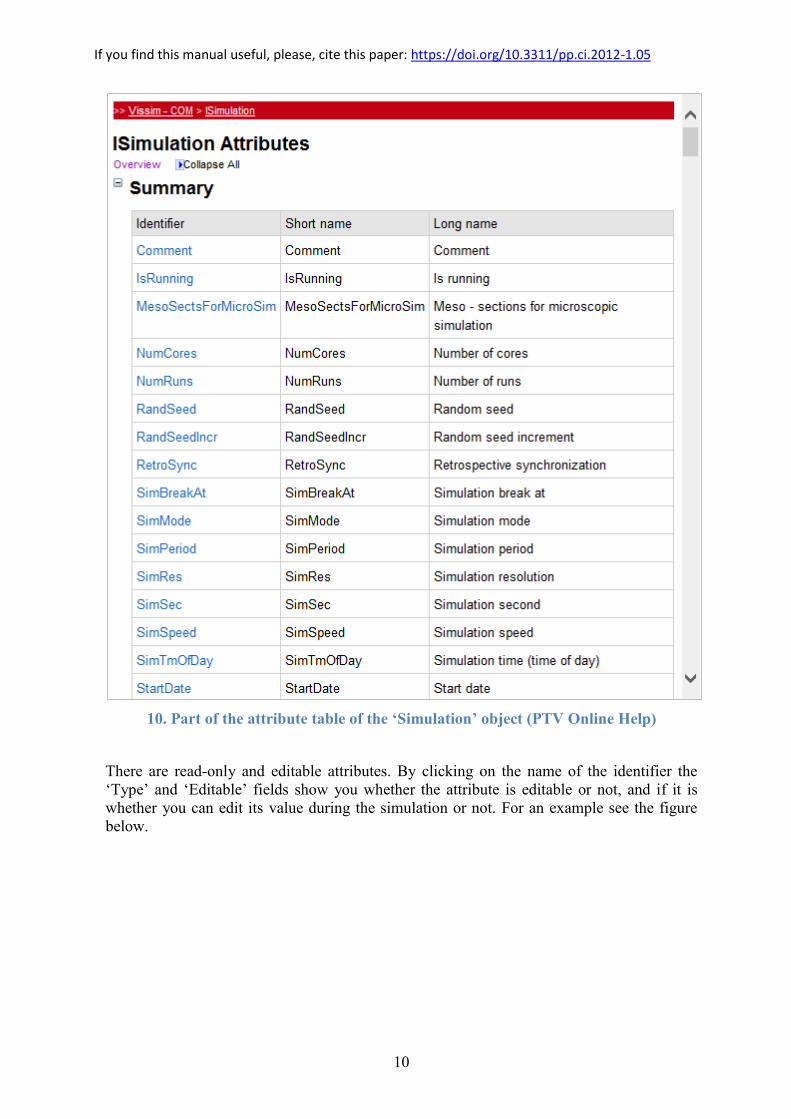
2. Object attributes

Objects have so-called attributes (‘Attribute’) as well. To reach them you must use the

‘AttValue’ method.

The attributes can be found in the Vissim Online Help via the Vissim GUI (click on

Help\Online Help…).

query of all the properties of the given object

(vis)

(sim)



10

10. Part of the attribute table of the ‘Simulation’ object (PTV Online Help)

There are read-only and editable attributes. By clicking on the name of the identifier the

‘Type’ and ‘Editable’ fields show you whether the attribute is editable or not, and if it is

whether you can edit its value during the simulation or not. For an example see the figure

below.



11

11. Editable and not editable attributes of ‘Simulation’

Syntax of the usage of the ‘AttValue’ method in the case of readout (‘get’) and for change

(‘set’) is as follows:

sim.get('AttValue', {'attribute'});

sim.set('AttValue', {'attribute'}, {adjustable value});

In connection with the figure above:

sim.get('AttValue', 'SimSec'); %(SimSec is read-only, so the ‘set’

command is not allowed.)

Another example to set the length of the simulation in Matlab Script file:

period_time=3600;

sim.set('AttValue', 'SimPeriod', period_time); %(You can edit it only outside the

simulation.)

sim.get('AttValue', 'SimPeriod') %(The answer will be 3600.)

As another example, we mention the ‘Simulation Resolution’ property. This represents

how many times the Vissim traffic model runs in a second during the simulation. We

can change it with the following code:

step_time=3;

sim.set('AttValue', 'SimRes', step_time); %(The ‘SimRes’ attribute can only

be set at full simulation seconds)

sim.set('AttValue', 'SimRes') %(The answer will be 3.)

There is an alternate syntax for reading Vissim attributes which is entirely equivalent to the

“get” method:

sim.AttValue({'attribute'});

An example is given below:

sim.AttValue('SimPeriod') ⟺ sim.get('AttValue', 'SimPeriod')



12

6. Running a simulation

Using Vissim there are three ways to run a simulation:

‘RunContinuous’: continuous running,

‘RunSingleStep’: running step-by-step, i.e. the time interval between steps will be

simulated according to the ‘Simulation Resolution’ setting,

‘RunMulti’: multiple simulations in a row.

We point out the ‘RunSingleStep’ method since this way makes it easy to manipulate the

simulation ‘online’, i.e. during the simulation run (for example changing the traffic demands

continuously).

‘RunSingleStep’ is recommended to use with a ‘for’ loop. In the following example we run a

simulation which shows the elapsed simulation time at each step (‘period_time’ and

‘step_time’ variables are defined previously).

for i=0:(period_time* step_time)

sim.RunSingleStep;

sim.get('AttValue', 'SimSec');

end

While using ‘RunSingleStep’, the ‘Simulation Speed’ setting has no effect on the running

speed of the simulation. In this case, the simulation runs step by step according to the ‘for’

loop, by running each ‘time step’ on the maximum speed is possible. Therefore, using the

above method the simulation speed can be controlled by Matlab ‘pause’ command (e.g. to

slow down the simulation for visual observation). In the following example, a 500 ms long

pause is inserted after each simulated time step:

for i=0:(period_time*step_time)

sim.RunSingleStep;

pause(0.5);

end

It must be noted that the ‘Snapshot’ functionality (for warm simulation start) has been totally

removed from version 7 of Vissim. The last version was Vissim 5 where ‘SaveSnapshot’ and

‘LoadSnapshot’ methods were included. The official site of PTV reports that this functionality

will be available in one of the future version of Vissim.



13

7. Traffic generation

Vissim-COM makes it possible to dynamically change traffic demands, which is very useful,

for example in the following cases:

to run several simulations with different traffic demands (possibly by ‘MultiRun’

method),

to generate varying traffic demand by following the traffic changes of a day (during

the simulation run).

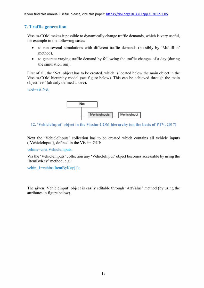
First of all, the ‘Net’ object has to be created, which is located below the main object in the

Vissim-COM hierarchy model (see figure below). This can be achieved through the main

object ‘vis’ (already defined above):

vnet=vis.Net;

12. ‘VehicleInput’ object in the Vissim-COM hierarchy (on the basis of PTV, 2017)

Next the ‘VehicleInputs’ collection has to be created which contains all vehicle inputs

(‘VehicleInput’), defined in the Vissim GUI:

vehins=vnet.VehicleInputs;

Via the ‘VehicleInputs’ collection any ‘VehicleInput’ object becomes accessible by using the

‘ItemByKey’ method, e.g.:

vehin_1=vehins.ItemByKey(1);

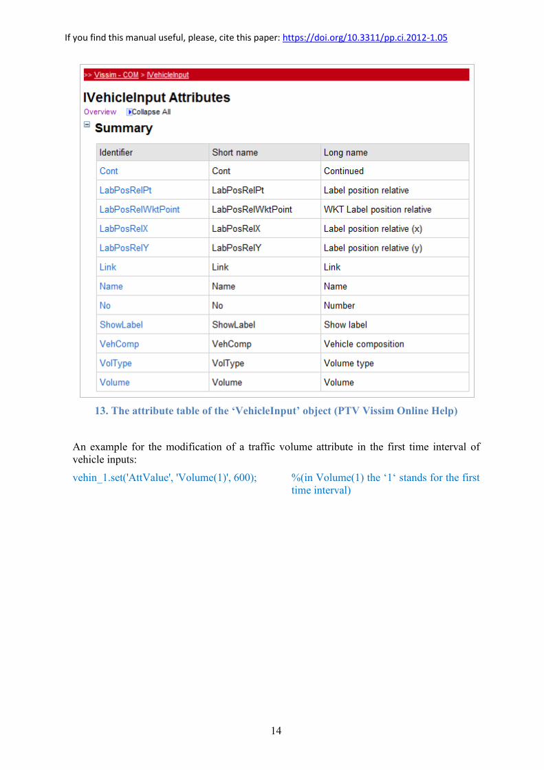
The given ‘VehicleInput’ object is easily editable through ‘AttValue’ method (by using the

attributes in figure below).



14

13. The attribute table of the ‘VehicleInput’ object (PTV Vissim Online Help)

An example for the modification of a traffic volume attribute in the first time interval of

vehicle inputs:

vehin_1.set('AttValue', 'Volume(1)', 600); %(in Volume(1) the ‘1‘ stands for the first

time interval)



15

8. Traffic signal control, detectors

Traffic light control can be programmed via COM interface as well. However, the previously

mentioned VisVAP module (flow chart based programming) or Signal Controller API

interface (on C++ language) can also be applied for traffic signal programming.

The traffic signal control within Vissim-COM object model is shown in the figure below.

14. Components of traffic signal control within Vissim-COM object model (on the

basis of PTV, 2017)

Now, a simple example is provided to demonstrate traffic signal control via Vissim-COM.

A simple signalized intersection is given (see the figure below), where two one-way roads (a

main road and a side street) meet. There are two signal groups operating in the junction. By

default, the main road is operated by a constant green time signal. At the same time, the signal

group of the side road only gets green time when the loop detector is activated. This is the so-

called demand-actuated traffic signaling. The system checks the loop detector’s availability

in every 20 seconds. The demand-actuated stage has 20 seconds.

15. Simple intersection in Vissim with traffic demand actuated control

Side street

Demand detector

Main road



16

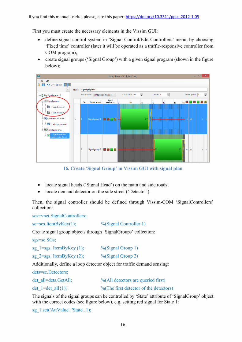
First you must create the necessary elements in the Vissim GUI:

define signal control system in ‘Signal Control/Edit Controllers’ menu, by choosing

‘Fixed time’ controller (later it will be operated as a traffic-responsive controller from

COM program);

create signal groups (‘Signal Group’) with a given signal program (shown in the figure

below);

16. Create ‘Signal Group’ in Vissim GUI with signal plan

locate signal heads (‘Signal Head’) on the main and side roads;

locate demand detector on the side street (‘Detector’).

Then, the signal controller should be defined through Vissim-COM ‘SignalControllers’

collection:

scs=vnet.SignalControllers;

sc=scs.ItemByKey(1); %(Signal Controller 1)

Create signal group objects through ‘SignalGroups’ collection:

sgs=sc.SGs;

sg_1=sgs. ItemByKey (1); %(Signal Group 1)

sg_2=sgs. ItemByKey (2); %(Signal Group 2)

Additionally, define a loop detector object for traffic demand sensing:

dets=sc.Detectors;

det_all=dets.GetAll; %(All detectors are queried first)

det_1=det_all{1}; %(The first detector of the detectors)

The signals of the signal groups can be controlled by ‘State’ attribute of ‘SignalGroup’ object

with the correct codes (see figure below), e.g. setting red signal for State 1:

sg_1.set('AttValue', 'State', 1);



17

17. ‘State’ attribute codes of ‘SignalGroup’ (PTV Vissim Online Help)

Status of the loop detector is queried also through the ‘AttValue’ method by various attributes

e.g.:

det_1.get('AttValue', 'Detection');

det_1.get('AttValue', 'Impulse');

det_1.get('AttValue', 'Occup'); %(Occupancy)

det_1.get('AttValue', 'Presence');

In addition to the above, the traffic-responsive logic is created by ‘rem’ command of Matlab

(which gives back the remainder after a division of two numbers):

for i=0:( period_time*step_time)

sim.RunSingleStep;

if rem(i/step_time,20)==0 % verifying at every 20 seconds

demand=det_1.get('AttValue', 'Presence'); % verifying detector occupancy: 0/1

if demand==1 % demand -> demand-actuated stage

sg_1.set('AttValue','State',1); % main road red (1)

sg_2.set('AttValue','State',3); % side street green (3)

else % no demand -> main road is green



18



end

end

end

So that it is easier to understand the logic, in the example above we neglected the intergreen

times between the two phases and we did not use transition signals (red-amber, amber). To

create them, further programming is necessary.



19

9. Evaluation while the program is running

An important advantage of the Vissim-COM is the possibility of evaluation while the program

is running. The following example is shown from the numerous evaluation options. We

consider the evaluation of data collection points through ‘DataCollectionMeasurements’.

Data Collection Points can be used effectively with the Vissim GUI. They can be positioned

on any link in the road network, furthermore they are suitable for measuring several

parameters in the given cross section (e.g. acceleration, number of vehicles, occupancy).

You can reach the measurements of the given data collection point through the ‘Data

Collection Measurements’ field and the ‘ItemByKey’ method:

datapoints=vnet.DataCollectionMeasurements;

datapoint1=datapoints.ItemByKey(1);

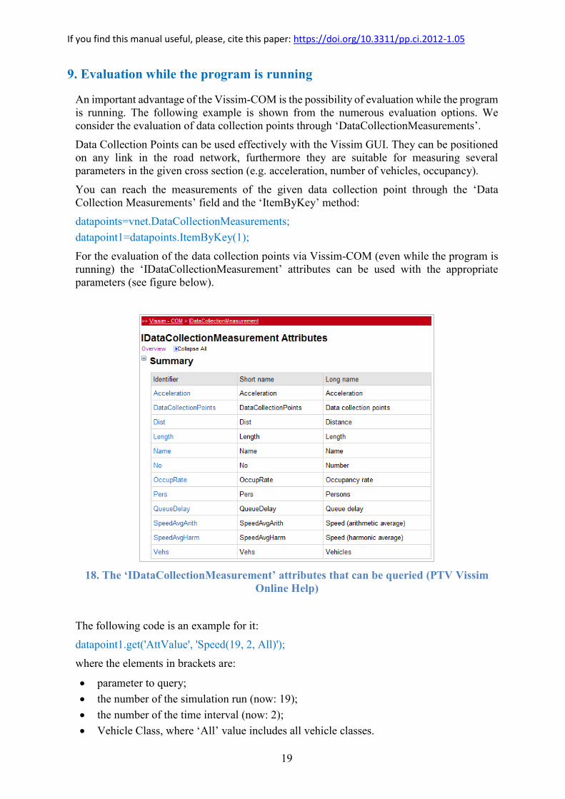
For the evaluation of the data collection points via Vissim-COM (even while the program is

running) the ‘IDataCollectionMeasurement’ attributes can be used with the appropriate

parameters (see figure below).

18. The ‘IDataCollectionMeasurement’ attributes that can be queried (PTV Vissim

Online Help)

The following code is an example for it:

datapoint1.get('AttValue', 'Speed(19, 2, All)');

where the elements in brackets are:

parameter to query;

the number of the simulation run (now: 19);

the number of the time interval (now: 2);

Vehicle Class, where ‘All’ value includes all vehicle classes.



20

Result attributes can be saved for multiple simulation runs, time intervals and different

vehicle classes. It is possible to access all saved result values by COM. To access these

values three sub attributes are required given in the figure below. You can replace the

constant (19 and 2 in the example above) sub-attributes with periodic inputs.

19. Sub-attributes’ table (PTV, 2017)

However, generally sub-attributes ‘Current’ and ‘Last’ (see their meaning in Fig. 19.) are

suggested to be used only, e.g. datapoint1.get('AttValue', 'Speed(Current, Last, All)');

An indispensable condition of measurement by data collection points is (even by using

Vissim-COM) that the option of ‘Data Collections\Collect data’ is flagged (and well

configured) in ‘Evaluation\Configuration…\Result Attributes’ menu in the Vissim GUI. The

time interval of data collections is also important. You will get an average value for the

measured factors in each time interval. The shorter the interval is the more sophisticated

results you get. The adjustment and the evaluation results are depicted in the figure below.

20. Evaluation configuration and evaluation results



21

10. A complete sample code for Vissim-COM programming

A sample code for Vissim-COM programming (written in Matlab) is presented below based

on the examples introduced in this manual.

%% Vissim-COM programming - example code %%

clear all;

close all;

clc; % Clears the command window

%% Create Vissim-COM server

vis=actxserver('VISSIM.vissim.900');

%% Loading the traffic network

access_path=pwd;

vis.LoadNet([access_path '\test.inpx']);

vis.LoadLayout([access_path '\test.layx']);

%% Simulation settings

sim=vis.Simulation;

period_time=3600;

sim.set('AttValue', 'SimPeriod', period_time);

step_time=3;

sim.set('AttValue', 'SimRes', step_time);

%% Define the network object

vnet=vis.Net;

%% Setting the traffic demands of the network

vehins=vnet.VehicleInputs;


vehin_1.set('AttValue', 'Volume(1)', 1500); % main road


vehin_2.set('AttValue', 'Volume(1)', 100); % side street

%% The objects of the traffic signal control

scs=vnet.SignalControllers;

sc=scs.ItemByKey(1);

sgs=sc.SGs; % SGs=SignalGroups

sg_1=sgs.ItemByKey(1);

sg_2=sgs.ItemByKey(2);

dets=sc.Detectors;

det_all=dets.GetAll;

det_1=det_all{1};

%% Access to DataCollectionPoint object

datapoints=vnet.DataCollectionMeasurements;

datapoint1=datapoints.ItemByKey(1);

%% Access to Link object

links=vnet.Links;

link_1=links.ItemByKey(1);

%% Running the simulation

verify=20; % verifying at every 20 seconds

%Evaluation\Configuration...\Interval in the Vissim GUI

for i=0:(period_time*step_time)

sim.RunSingleStep;

if rem(i/step_time, verify)==0 % verifying at every 20 seconds

demand=det_1.get('AttValue', 'Presence'); %get detector occupancy:0/1

if demand==1 % demand -> demand-actuated stage

sg_1.set('AttValue', 'State', 1); % main road red (1)

sg_2.set('AttValue', 'State', 3); % side street green (3)

else % no demand on loop -> main road's signal is green



end

% Query the avg. speed and vehicle number at the end of each eval. interval:

datapoint1.get('AttValue', 'Vehs(Current, Last, All)')

datapoint1.get('AttValue', 'Speed(Current, Last, All)')

end

end

%% Delete Vissim-COM server (also closes the Vissim GUI)

vis.release;

disp('The end')



22

11. Bibliography

Box D. Essential COM, Addison-Wesley, ISBN 0-201-63446-5, 1998

PTV, Introduction to the PTV Vissim 9 COM API, PTV Planung Transport Verkehr AG,

Germany, 2017

Wiedemann R. Simulation des Straßenverkehrsflusses Schriftenreihe des Instituts für

Verkehrswesen der Universität Karlsruhe, Heft 8, 1974


a practical manual for vissim com programming in matlab · as well. the principle of com...

Documents