a practical guide to fitting p* social network models via logistic regression€¦ · ·...

A Practical Guide To Fitting p* Social Network Models Via Logistic Regression

Bradley Crouch and Stanley Wasserman∗ University of Illinois

WORK IN PROGRESS – COMMENTS WELCOME

∗ Funding provided by a National Science Foundation Graduate Research Fellowship and a National Science Foundation grant (#SBR96-30754) to the University of Illinois. Correspondence can be addressed to Brad Crouch, 437 Psychology Building, 603 E. Daniel Street, Champaign, IL 61820 or to [email protected].

12

3 6

4

5

A Practical Guide to Fitting p* 2

Last Revised: June 18, 1997


Preface

To date, no single piece of software has been introduced that meets all the needs of the p* modeller. Thus, it is the purpose of this collection of papers, software and practical comments to bring together some of the pieces necessary for the applied researcher to preprocess network data, fit pseudolikelihood versions of p* models, and interpret the results. Although this compilation is intended to be fairly self-contained with respect to computational issues surrounding p*, it is assumed that reader has reviewed the theoretical development of these models by Wasserman & Pattison (1996).


Table of Contents

Example File Descriptions .................................................................................................................4 Linear Regression Review ..................................................................................................................5 A Regression Model For Binary Responses ....................................................................................7 The Basics Of Logistic Regression ...................................................................................................8 Assessing The Fit Of A Logistic Regression Model ......................................................................9 A Small Artificial Network Dataset ................................................................................................10 The Logit p* Representation ...........................................................................................................11 Model Fitting With Logistic Regression ........................................................................................12 The MDS CRADA Network ..........................................................................................................19 Preprocessing Network Data With PREPSTAR .........................................................................20 Some Model Comparisons Using SAS ...........................................................................................23 Summary ...........................................................................................................................................XX References ..........................................................................................................................................24 Appendices: Ardu, S. (1995). Setup (PREPSTAR) manual. .............................................................XX

<<not yet included -- need to revise & update blocking section>>

Example File Descriptions (On Included Disk)

PREPSTAR.EXE: A DOS utility to preprocess sociomatrices into a form suitable for most statistical packages, including SAS and SPSS.

6ACTOR.NET: The PREPSTAR input file containing the sociomatrix and blocking information for the fictitious six-actor network used throughout this guide.

6ACTOR.SAV: An SPSS data file in logistic regression format for the six-actor network.

CRADA.DL: Valued sociomatrix for the CRADA data example ready for import into current versions of UCINET IV1.

CRADA01.KP: KrackPlot2 input file for the dichotomized CRADA dataset.

CRADA01.NET: PREPSTAR input file for the dichotomized CRADA dataset.

CRADA01.SAS: SAS program for fitting the series of models to the CRADA network as described in this guide—includes all explanatory variables computed by PREPSTAR.

CRADA01.SAV: SPSS data file in logistic regression format for the CRADA network.

GUIDE.DOC: This document in MS Word 7.0 For Windows 95 format (formatting may depend on system configuration and printer).

GUIDE.PS This document in postscript format (recommended).

1 Information on obtaining UCINET is available at http://eclectic.ss.uci.edu/~lin/ucinet.html. 2 Information on obtaining KrackPlot is available at www.heinz.cmu.edu.


Linear Regression Review

Before we move into logistic regressions and p* social network models, let us review some basic concepts from a more familiar technique, linear regression analysis (for a full treatment of this topic, see Weisberg (1985)). One goal in regression analysis is to relate potentially “important” explanatory variables to the response variable of interest. Formally, the basic model states, Yi = β0 + β1 xi1 + β2 xi2 + ... + βp xip + εi (1) where Yi is the response for the i th case, i=1,2,...,n (number of cases) xi1, xi2, ..., xip are the explanatory variables for the ith case and β0, β1, ..., βp are regression coefficients, or model parameters, to be estimated. Without detailing the computations, estimates of the β coefficients can be found such that the sum of the squared differences between the observed responses (Yi ) and the responses predicted by the model ( $Yi ) is at a minimum. More formally, the least squares estimates of the regression coefficients minimize the quantity,

( $ $Y Y ) SSEi ii

n

ii

n

− = == =∑ ∑2

1

2

1ε (2)

and are usually termed $β . Of course, the $Yi terms are obtained by “plugging” the observed values of the explanatory variables into the estimated regression function, $Yi = $β 0 + $β 1 xi1 + $β 2 xi2 + ... + $β p xip (3) If the model fits the observed data well, then the sum of squared errors is small relative to the total variation in the response. The “degree” of model fit is often captured by the index, R2. Note than when the model fits perfectly, SSE=0, and R2=1. One can glean some information about the importance of each explanatory variable from a regression by inspecting the sign and magnitude of the estimated regression coefficients. In general, the model states that the response Yi changes by a factor of βj when the j th explanatory variable increases by one unit while the remaining explanatory variables are held constant. Since the explanatory variables are often measured on different scales, the magnitude of these coefficients reflect as much about the scale of the data and about the presence or absence of other correlated predictor variables as they convey about the importance of the predictor. Therefore, an alternative strategy of comparing model fit is often used to “tease out” the importance of each explanatory variable. For instance, consider two models relating


Y= Graduate GPA to the explanatory variables, x1 = Undergrad GPA x2 = GRE Scores x3 = Interview Score. Suppose we fit the full model that includes all three predictor variables and find that it fits quite well with an R2=0.81. Our hypothesis, however, might be that interviews of prospective graduate students do not account for an appreciable amount of the variance in GPA. Thus, one might wish to test the hypothesis,

Ho: β3 = 0 (no linear relationship between Interview scores & GPA given the presence of the other explanatory variables are in the model)

H1: β3 ≠ 0 This amounts to comparing the fit of the full model against a reduced model that does not include a parameter for the Interview explanatory variable, i.e. Full Model: Yi = β0 + β1 xi1 + β2 xi2 +β3 xi3 + εi Reduced Model: Yi = β0 + β1 xi1 + β2 xi2 + εi Given independence and normality assumptions about the errors, well-known theory tells us that the difference in fit between the two models follows an F distribution with numerator degrees of freedom equal to the difference in the degrees of freedom of the full versus reduced models (dfF - dfR) and denominator degrees of freedom equal to n-p-1. Thus, we can compute the observed F-value via the formula,

(4)

and compare it to an F distribution with the appropriate degrees of freedom. If the result is statistically significant, then one can conclude that setting the Interview parameter to zero results in an appreciable loss of fit, suggesting that this explanatory variable should be retained in our model. Conversely, if the observed F statistic is not significant, one may choose to adopt the more parsimonious 2-predictor model. Although the details differ, we will use this same strategy to evaluate the logistic regression models throughout this guide. A Comment on Notation It is often convenient to develop a more compact notation to discuss regression models. In vector notation, model (1) can be restated for the ith case as, Yi = xi

Tβ + εi (5)

FR R df df

R dfObSF R R F

F F

=− −−

( ) / ( )( ) /

2 2

21


where xiT = ( 1 xi1 xi2 ... xip ) and βT = ( β0 β1 β2 ... βp ). Of course, the use of Yi , x and β to represent the response, the vector of explanatory variables and the parameter vector, respectively, is a matter of convention. We could have just as well defined Xi = zi

Tθ + εi. This latter notation more closely corresponds to that used from this point forward. A Regression Model For Binary Responses Turning back to the previous regression model for Graduate GPA, suppose that members of the graduate admission committee are less interested in predicting prospective student grades, but are more concerned with predicting the completion, or lack thereof, of the PhD dissertation. This new response, denoted by Xi, can take on only two values of 1=“Completed” or 0=“Not Completed”. For simplicity, let us consider the relationship of the response to a single explanatory variable, z 1 = “Undergraduate GPA”. With continuous variables, a scatterplot is commonly used to visualize the relationship between the response and an explanatory variable. In the case of this binary response, however, a scatterplot of the zi versus the Xi would result in two horizontal bands of points at both X = 1 and X = 0. Thus, in order to generate a more meaningful plot and summarize the data in a more meaningful way, let us group the observations into intervals based on the

GPA of the cases and consider the proportion of dissertation completions within each GPA group. The resulting plot might look like the one to the left. We now have a plot of the empirical probabilities of completing the dissertation as a function of “grouped” GPA and can now study the linear relationship between the two variables. But, note that the linear regression line demonstrates some serious flaws in using linear models for binary responses. Perhaps the most obvious of these is the fact that for sufficiently large or small values of the explanatory variable, the model predicts values outside of the [0,1] range of the response.

Further, one might notice that there appears to be a different relationship between z and X at different levels of z. A small increase in grade point at the middle values of GPA has a high impact on the proportion of those completing their dissertation. On the other hand, it appears that for students is in the two highest GPA intervals, the proportion of students that

GPA1 2 3 4

Pr(Completion)

0.25

0.50

0.75

1.00

X

X

X

X

XX


complete the dissertation changes little since the proportion is near the maximum value of the response, unity. Agresti (Ch. 4, 1990) cites other more technical defects in linear models for probabilities including the sub-optimality of least squares estimators, failure of the homoscedasticity assumption, and the lack of normally distributed errors. Altogether then, it appears that a different type of regression model is needed for binary data, and in particular, for dichotomous social relations.

The Basics Of Logistic Regression Another look at the previous plot suggests not a linear, but a curvilinear relationship between GPA and dissertation completion. Thus, instead of fitting a straight line to the data, a special type of curve can be used to model the relationship between the explanatory variable and the response. This curve can be described by a function of a set of parameters (parameters not unlike the β coefficients in (1)). Here, however, the function relating the explanatory variable to the response is nonlinear, and is of the form,

(6)

and is called the logistic regression function. This model can be reformulated into a linear model by considering the log odds of the response, or the log of the ratio of the probability that the response equals one to the probability that it equals zero, or

. (7)

Notice that the response, X, has been transformed from a variable that ranges between one and unity to a variable called a logit that ranges from -∞ to +∞. When the responses zero and one are equally likely, the logit equals zero, but is positive when one is the more probable outcome and negative when zero is more probable.

GPA1 2 3 4

Pr(Completion)

0.25

0.50

0.75

1.00

X

X

X

X

XX

Pr ( ) exp( )exp( )

X zz

= =+

+ +1

10 1 1

0 1 1

θ θθ θ

logPr ( )Pr ( )

XX

z==

= +

10 0 1 1θ θ


A third formulation of the logistic regression model provides a possibly more intuitive interpretation of the θ coefficients. Rather than considering the natural logarithm of the odds that the response is unity, one can consider the odds ratio itself, or

(8)

Thus, for a unit increase in the explanatory variable z1, the odds ratio that the response equals one changes by a factor of exp(θ1). In our example, if θ1=.69315, the model would predict that an increase of one in Undergraduate GPA would increase the odds of dissertation completion by a factor of exp(.69315)=2. Further, one can compute the predicted probability of dissertation completion given the student’s GPA from (6). If θ0=0.2, θ1=0.69135, and z i1=3.0, the model predicts that

.

Of course, we have yet to determine if these probabilities predicted by the model correspond well to the observed data. Thus, we now turn to a summary of techniques useful for assessing model fit. Assessing The Fit Of A Logistic Regression Model As described earlier, R2 is a natural measure of fit for linear regression models as it is directly related to the least squares criterion used to obtain the “best” estimates of the regression parameters. Logistic regression coefficients are estimated by maximum likelihood, using a an iteratively reweighted least squares computational procedure. The “natural” measure of model fit is given by the maximized log likelihood of the model given the observed data, and denoted by L. Recall that we can compare the fit of two linear regression models using (4). Similarly, we can compare the fit of two logistic regression models by inspecting the likelihood ratio statistic, LR = -2(LR - LF), where LF is the log likelihood of the full model and LR is the log likelihood of the reduced model (obtained by setting q of the parameters in the full model to zero). When the full model “fits” and the number of observations is large, LR is distributed as a chi-squared random variable with q degrees of freedom. Therefore, if the difference in fit between two models is small relative to the χ2

q distribution, one can adopt the model with fewer parameters without suffering an appreciable loss of fit. A discussion of other fit measures is found later in this guide.

Pr ( )Pr ( )

exp ( ) ( )XX

z e e z==

= + =10 0 1 1

0 1 1θ θ θ θ

Pr ( )exp ( . . . )

exp ( . . . ).X i = =

+ ∗+ + ∗

≈10 2 69315 3 0

1 0 2 69315 3 00 91


Guided by the discussion in this section and intuition already developed for linear regression models, we have the basic components necessary to estimate, test the fit of, and interpret logistic regression models for binary responses. We now turn to a class of models for the binary response of interest in this guide, a social network relational tie.

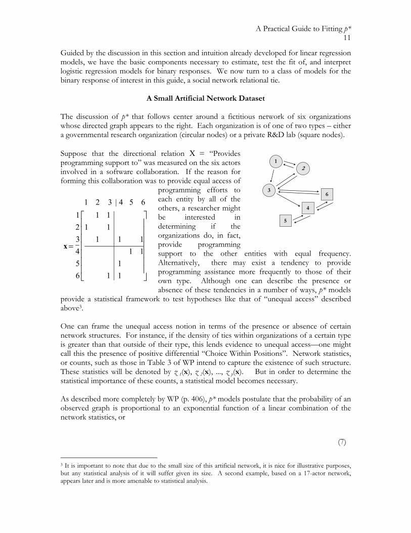
A Small Artificial Network Dataset

The discussion of p* that follows center around a fictitious network of six organizations whose directed graph appears to the right. Each organization is of one of two types – either a governmental research organization (circular nodes) or a private R&D lab (square nodes). Suppose that the directional relation X = “Provides programming support to” was measured on the six actors involved in a software collaboration. If the reason for forming this collaboration was to provide equal access of

programming efforts to each entity by all of the others, a researcher might be interested in determining if the organizations do, in fact, provide programming support to the other entities with equal frequency. Alternatively, there may exist a tendency to provide programming assistance more frequently to those of their own type. Although one can describe the presence or absence of these tendencies in a number of ways, p* models

provide a statistical framework to test hypotheses like that of “unequal access” described above3. One can frame the unequal access notion in terms of the presence or absence of certain network structures. For instance, if the density of ties within organizations of a certain type is greater than that outside of their type, this lends evidence to unequal access—one might call this the presence of positive differential “Choice Within Positions”. Network statistics, or counts, such as those in Table 3 of WP intend to capture the existence of such structure. These statistics will be denoted by z 1(x), z 2(x), ..., z p(x). But in order to determine the statistical importance of these counts, a statistical model becomes necessary. As described more completely by WP (p. 406), p* models postulate that the probability of an observed graph is proportional to an exponential function of a linear combination of the network statistics, or

3 It is important to note that due to the small size of this artificial network, it is nice for illustrative purposes, but any statistical analysis of it will suffer given its size. A second example, based on a 17-actor network, appears later and is more amenable to statistical analysis.

12

3 6

4

5

1 2 3 4 5 6123456

1 11 1

1 1 11 1

11 1

|

x =

(7)


where θ is the vector of model parameters and z(x) is the vector of network statistics. For example, suppose that one element of z(x) is a count of the number of ties within positions and the θ parameter corresponding to the count is large and positive. Such a model predicts that networks with a large number of within position ties will be observed with a higher probability than those with a lesser number of within position ties (see also, WP p. 415 for more on model interpretation). Of course, in practice, the θ parameters are not known a priori and must be estimated. Due to the difficulty in analytically specifying the κ (θ ) term in the probability function (7), the model does not lend itself well to maximum likelihood estimation. Fortunately, the model can be reformulated in logit terms and fitted approximately by logistic regression—a strategy to be summarized next.

The Logit p* Representation

As more fully laid out by WP, the log linear form of p* given by (7) can be reformulated as a logit model for the probability of each network tie, rather than the probability of the sociomatrix as a whole. First, WP defines three new sociomatrices,

Xij+: the sociomatrix for relation X where the tie from actor i to actor j is

forced to be present.

Xij-: the sociomatrix for relation X where the tie from actor i to actor j is

forced to be absent.

XijC: the sociomatrix of the complement relation for the tie from i to j. This

complement relation has no relational tie coded from i to j-- one can view this single tie as missing.

By conditioning on the complement relation, some algebra (WP, p 407) yields a logit model for the probability of each network tie as a function of the explanatory variables, or

(8)

The expression δ(xij ) is the vector of changes in network statistics that arises when the tie Xij changes from a 1 to a 0. The similarity between this formulation, termed logit p*, and the logit version of the logistic regression model (4) is apparent, suggesting that logistic regression is a suitable estimation technique.

{ }Pr( ) exp{ ( )}( )

exp ( ) ( ) ... ( )X x z x x x x= =′

∝ + + +θκ θ

θ θ θ1 1 2 2z z zp p

ϖ θ θ δijij ij

c

ij ijc ij ij ij

XX

x==

=

= ′ − = ′+ −log

Pr( | )Pr( | )

[ ( ) ( )] ( )10XX

z x z x


Statistical interpretation of logistic regression models, however, depends on the assumption that the logits are independent of one another. In the case of p*, the logits are clearly not independent. Therefore, measures such as the likelihood ratio statistic do not carry a strict statistical interpretation, but are useful as a liberal guide for evaluating model goodness-of-fit. Armed with a basic understanding of logit p*, we can now proceed to a more practical discussion of the steps necessary to fit the model to our fictitious network of six organizations. Model Fitting With Logistic Regression

Suppose, for example, we are considering a model with parameters for overall degree of Choice (θ), Differential Choice Within Positions (θW), Mutuality(ρ), Differential Mutuality Within Positions (ρW), and Transitivity (τT). Thus, the vector of model parameters to be estimated is θ = { θ θW ρ ρW τT }.

In order to compute the vector of explanatory variables, δ(xij), that consists of elements corresponding to each of the parameters, we examine each xij, for all i,j=1, 2,..., n, i≠j, and compute the change in the vector of network statistics, z(x), when the tie between i and j changes from a 1 to a 0. First, as defined by WP (p 407), we recall that δ(xij) = [z(xij

+ ) - z(xij- )]

= {z1(xij+ ) - z1(xij

- ), z2(xij+ ) - z2(xij

- ), z3(xij+ ) - z3(xij

- ), z4(xij+ ) - z4(xij

- ), z5(xij+ ) - z5(xij

-

)} where, in our case (based on WP Table 3), z1(x) = L = Σi,j Xij is the statistic for the Choice parameter, θ, z2(x) = LW = Σi,j Xij δij is the statistic for the Choice Within Positions parameter, θW, z3(x) = M = Σi<j Xij Xji is the statistic for the Mutuality parameter, ρ,

z4(x) = MW = Σi<j Xij Xji δij is the statistic for the Mutuality Within Positions parameter, ρW,

and z5(x) = TT = Σi,j,k Xij Xjk Xik is the statistic for the Transitivity parameter, τT. Note that the indicator variable δij=1 if actors i and j are in the same position, and 0 otherwise.


So, to demonstrate the computations, let us first consider the tie x12. We can compute the explanatory variable for Choice by considering the difference in z1(x) when the tie is present versus when it is absent. In other words,

∆L = z1(xij+) - z1(xij

-) = L(xij+) - L(xij

-) = 12 -11 = 1. Similarly, the change in z3(x) is the difference in the number of mutual ties when x12 goes from 1 to 0, or

∆M = z3(xij+ ) - z3(xij

- ) = M(xij+ ) - M(xij

- ) = 5 - 4 = 1. The change in z4(x) is computed somewhat differently as one only counts the number of mutual ties between actors in the same position. Since actors 1 and 2 are “blocked” together and have a mutual tie, the change in MW equals the change in M:

∆MB = z4(xij+ ) - z4(xij

- ) = MB(xij+ ) - MB(xij

- ) = 5 - 4 = 1. Note, however, that for the tie x36, ∆MB=0 despite the fact that the tie between actors 3 and 6 is mutual. Since they are not in the same position, the indicator variable δij=0, thus this mutual tie is not counted. Of course, one can continue this process for all five explanatory variables for all off-diagonal elements in x. Fortunately, the C program PREPSTAR (Ardu, 1995) performs these calculations for a host of network statistics and sociomatrices of any size. Listed below is an excerpt from PREPSTAR output (see the section on preprocessing network data for more detail). The output consists of g(g-1) lines, each containing the actor indices i and j, the observed tie between them, and the vector of explanatory variables. Obs i j tie L L_W M M_W T_T --- --- --- --- --- --- --- --- --- 1 1 2 1 1 1 1 1 2 2 1 3 1 1 1 0 0 3 3 1 4 0 1 0 0 0 1 4 1 5 0 1 0 0 0 0 5 1 6 0 1 0 0 0 2 6 2 1 1 1 1 1 1 1 7 2 3 1 1 1 1 1 2 8 2 4 0 1 0 0 0 2 9 2 5 0 1 0 0 0 0 10 2 6 0 1 0 0 0 3 11 3 1 0 1 1 1 1 3 12 3 2 1 1 1 1 1 1 13 3 4 1 1 0 0 0 3 14 3 5 0 1 0 0 0 2 15 3 6 1 1 0 1 0 2 16 4 1 0 1 0 0 0 0 17 4 2 0 1 0 0 0 1 18 4 3 0 1 0 1 0 3 19 4 5 1 1 1 1 1 0 20 4 6 1 1 1 1 1 1 21 5 1 0 1 0 0 0 0 22 5 2 0 1 0 0 0 0 23 5 3 0 1 0 0 0 1 24 5 4 1 1 1 1 1 0 25 5 6 0 1 1 0 0 3 26 6 1 0 1 0 0 0 1


27 6 2 0 1 0 0 0 3 28 6 3 1 1 0 1 0 1 29 6 4 1 1 1 1 1 2 30 6 5 0 1 1 0 0 3

Text such as this is easily imported into most statistical packages, including SAS and SPSS. For demonstration purposes, these data were imported into SPSS-- the resulting SPSS data file is saved under the name 6ACTOR.SAV on the included disk. A total of four models were considered ranging from the largest model that contains all the explanatory variables described above to the simplest of models containing only a parameter for Choice. Output from each of these regressions appears next. A guide to interpreting the SPSS output follows the first model and an overall summary of the results precedes the close of this section. Model 1: Choice + Choice Within Positions + Mutuality + Mutuality Within Positions + Transitivity -2 Log Likelihood 20.893 [1] Goodness of Fit 42.368 [2] Chi-Square df Significance Model Chi-Square 20.696 5 .0009 [3] Improvement 20.696 5 .0009 Classification Table for TIE [4] Predicted 0 1 Percent Correct 0 I 1 Observed +-------+-------+ 0 0 I 16 I 2 I 88.89% +-------+-------+ 1 1 I 2 I 10 I 83.33% +-------+-------+ Overall 86.67% ---------------------- Variables in the Equation ----------------------- [5] [6] [7] [8] [9]] [10] Variable B S.E. Wald df Sig R Exp(B) L -2.2079 1.1968 3.4036 1 .0651 -.1837 .1099 L_W 2.7390 2.1829 1.5744 1 .2096 .0000 15.4709 M 3.7356 1.8281 4.1755 1 .0410 .2287 41.9139 M_W -1.5861 2.9205 .2949 1 .5871 .0000 .2047 T_T -.4081 .6895 .3502 1 .5540 .0000 .6649 Correlation Matrix: [11] Constant L_B M M_BLK T_T Constant 1.00000 -.08007 -.26511 .00392 -.49406 L_W -.08007 1.00000 .58598 -.82404 -.67675 M -.26511 .58598 1.00000 -.77846 -.46499 M_W .00392 -.82404 -.77846 1.00000 .61903 T_T -.49406 -.67675 -.46499 .61903 1.00000 Interpreting The Output


The discussion below refers to each of the 12 bold markers (e.g.[1]) in the preceding output. For more detail, see the SPSS documentation. [1]. This is twice the negative of the log likelihood for the model. Note, that as a model model fits better, -2L decreases. . If the model were to fit perfectly, the likelihood would equal one and -2L would equal zero. Thus, this is a “badness of fit” measure—large values suggest poor fit. [2]. This goodness of fit measure is based on the residuals, or the difference between the observed responses xij and the probabilities predicted by the model, $xij , and defined as

[3]. The difference between -2L for the model and -2L for a model with all parameters for all explanatory variables set to 0. [4]. This table crossclassifies the observed response with the response predicted by the model (if $xij >.50 then the predicted response is set to 1, else it is set to 0). [5]. The parameter estimate for the explanatory variable listed on the left. In terms of the

log linear form of p*, a large positive value of a parameter suggests the presence of the associated network structural component (such as Mutuality), while a large negative value suggests its absence. Since the explanatory variables are measured on different scales, the notion of a “large” or “small” value is not especially well-defined. Thus, in order to determine a single parameter’s contribution to the overall likelihood, one can fit a smaller model without the parameter and inspect the increase in -2L, as previously discussed. Dually, one can interpret the parameters in terms of logit p*. For instance, as the number of transitive triads involving the tie from actor i to actor j increases by one, and the other explanatory variables remain constant, the odds that i sends a tie to j increase by a factor of exp(τ)=0.6649 (from the column labeled [10]).

[6]. The estimated asymptotic standard error of the parameter estimate. With network data, these standard errors are known to be too narrow, thus should not be strictly interpreted. [7]. The Wald statistic, defined as {(parameter estimate)/SE(parameter estimate)}2. For large sample sizes, this statistic is distributed as a chi-squared random variable with one degree of freedom. It is generally agreed (e.g. Agresti, 1990) that this statistic can be poorly behaved when the estimate is large, thus comparing two model likelihoods (as discussed in [5]) is the suggested strategy.

Zx x

x xij ij

ij iji

g g2

1

1

1=

−

−=

−

∑( $ )$ ( $ )

( )


[8] & [9]. Degrees of freedom and p-value for the Wald statistic. [10]. See [5]. [11]. The matrix of correlations of the parameter estimates. While it is expected that the parameters will be often be correlated, correlations of very large magnitude (either positive or negative) suggest that the parameters are not only accounting for very similar effects, but may lead to numerical instability of the estimation procedure. Thus, guided by theory, it is advisable to reconsider the choice of explanatory variables such that they capture more distinct structural elements in the network. Model 2: Choice + Choice Within Positions + Mutuality + Mutuality Within

Positions -2 Log Likelihood 21.265 Goodness of Fit 29.997 Chi-Square df Significance Model Chi-Square 20.324 4 .0004 Improvement 20.324 4 .0004 Classification Table for TIE Predicted 0 1 Percent Correct 0 I 1 Observed +-------+-------+ 0 0 I 16 I 2 I 88.89% +-------+-------+ 1 1 I 2 I 10 I 83.33% +-------+-------+ Overall 86.67% ---------------------- Variables in the Equation ----------------------- Variable B S.E. Wald df Sig R Exp(B) L -2.6388 1.0350 6.5005 1 .0108 -.3290 .0714 L_W 1.9456 1.6035 1.4723 1 .2250 .0000 6.9981 M 3.3319 1.6035 4.3178 1 .0377 .2361 27.9926 M_W -.5594 2.2795 .0602 1 .8062 .0000 .5716 Model 3: Choice + Mutuality -2 Log Likelihood 23.371 Goodness of Fit 30.000 Chi-Square df Significance Model Chi-Square 18.217 2 .0001 Improvement 18.217 2 .0001 Classification Table for TIE Predicted 0 1 Percent Correct 0 I 1 Observed +-------+-------+ 0 0 I 16 I 2 I 88.89%


+-------+-------+ 1 1 I 2 I 10 I 83.33% +-------+-------+ Overall 86.67% ---------------------- Variables in the Equation ----------------------- Variable B S.E. Wald df Sig R Exp(B) L -2.0794 .7500 7.6872 1 .0056 -.3698 .1250 M 3.6889 1.0782 11.7057 1 .0006 .4831 39.9999 Model 4: Choice -2 Log Likelihood 40.381 Goodness of Fit 30.000 Chi-Square df Significance Model Chi-Square 1.208 1 .2717 Improvement 1.208 1 .2717 Classification Table for TIE Predicted 0 1 Percent Correct 0 I 1 Observed +-------+-------+ 0 0 I 18 I 0 I 100.00% +-------+-------+ 1 1 I 12 I 0 I .00% +-------+-------+ Overall 60.00% ---------------------- Variables in the Equation ----------------------- Variable B S.E. Wald df Sig R Exp(B) L -.4055 .3727 1.1837 1 .2766 .0000 .6667 Summary: Model

Number of Parameters

-2L 4. Choice 1 40.38 3. Choice + Mutuality 2 23.37 2. Choice + Mutuality + Choice Within Positions +

Mutuality Within Positions 4 21.27

1. Choice + Mutuality + Transitivity + Choice Within Positions + Mutuality Within Positions

5 20.89

Inspection of -2L for Model 4 versus Model 3 reveals a large difference in fit, lending evidence to the importance of mutuality to the network. The parameter estimate is 3.6889, suggesting a very strong overall tendency for relational ties to be reciprocated. A glance at the directed graph presented earlier confirms this trend as there are clearly a large number of mutual ties as compared to non-mutual ties.


Now recall the ‘unequal access’ hypothesis from the description of 6-actor network. It was conjectured that organizations may tend to support the programming efforts of other organizations of their own type more often than those of other types. Inspection of -2L suggests that Models 1-3 do not differ greatly with respect to overall fit, lending evidence against both the presence of differential choice within positions and a tendency for (or against) the transitivity of ties. Thus, it appears that there is no strong evidence to conclude that these fictitious organizations tend to differentially support those in either network position. Further, it is clear that programming support is often reciprocated.


The MDS CRADA Network Note to network seminar members: Eventually an analysis of the CRADA dataset will be outlined here. To support the homework assignment, I have included a description of the dataset provided by Nosh and instructions on the procedure for preprocessing the data and importing it into SAS, but I did not include the analysis itself for the time being. Little is understood about the social and organizational issues surrounding "virtual work communities" – the growing global trend toward strategic business alliances that rely on high levels of interactive computer-based communication – but that is changing. Research being conducted by faculty at the University of Illinois at Urbana-Champaign and the University of Southern California is beginning to shed light on how communication-intensive communities can be most effective. The community under study is composed of representatives from three agencies of the US Army and four private corporations who have forged a Cooperative Research and Development Agreement (CRADA). Ultimately, this CRADA will lead to the commercial production of software for improving the building design process for large institutional facilities. The four private companies are Bentley Systems Inc., Exton, Pa., a CAD operating systems developer; Building Systems Design Inc., Atlanta, Ga., a construction software firm; IdeaGraphix Inc., Atlanta, Ga., a software development company; and JMGR Inc., Memphis, Tenn., an architectural firm. The US Army partners include Construction Engineering Research Laboratories, Champaign, Ill.; Corps of Engineers, Louisville District; US Army Reserve, and US Army Corps of Engineers Headquarters, Washington, D.C. The software to be produced through this CRADA is itself a contributor to virtual communities among planners, architects, cost estimators, and builders of major facilities in the private sector. The software will offer advanced “virtual” coordination capabilities through its object-oriented technology and modular design system (MDS).

CRADAs, which were first authorized by the 1986 Technology Transfer Act, enable government and industry to negotiate patent rights and royalties before entering into joint research and development projects. They were conceived as an incentive for industry, to facilitate investment in joint research by reducing the risk that the products of the research would fall into the public domain and be exploited by both domestic and international competitors. Since 1989, there has been an exponential growth in the creation of CRADAs, reaching over 2,200 by 1993. A large proportion of these were initiated by the departments of Energy, Commerce, Agriculture and Defense. They were signed with large, medium and small businesses in a wide variety of industries, including computer software, materials, agricultural chemicals, biomedical research and electronic networking. Unlike the complex MDS CRADA that is the subject of this research, most other CRADAs involve only one partner from private industry. The MDS CRADA is a particularly important advance because the organizations needed not only to hammer out an agreement with the multiple government agencies, but also to work through the difficult process of negotiating an agreement for how their own partnership is to function and how the benefits of the alliance are to be distributed among the partners. After a complex set of negotiations, a partnership framework was developed among the business participants, and the CRADA agreement was signed in a ceremony in Washington D. C. on July 18.


Preprocessing Network Data With PREPSTAR

As previously mentioned, PREPSTAR takes a square sociomatrix, computes values of many explanatory variables for each tie and outputs a data matrix suitable for import to statistical packages. For a full description of the program’s capabilities, consult the appendix. Listed below is the PREPSTAR input file for the dichotomized CRADA dataset at Time 9, a script detailing the prompts from PREPSTAR, and a snipped version of the output. The input file below, CRADA01.NET, includes the sociomatrix and actor position information (note that PREPSTAR currently refers to positions as “blocks”). Comments appear in bold and are for illustration only, thus they must not be included in the input file. Further, the only blank line in the file must follow the sociomatrix.

To execute the program, type prepstar.

CRADA (Dichotomized) - Time 9 //title line 0 1 1 1 0 0 1 1 1 0 1 1 0 0 0 0 0 1 0 1 0 0 0 0 0 0 0 0 0 0 0 0 0 0 1 1 0 0 1 0 1 1 0 0 1 0 0 1 0 1 1 1 0 0 0 1 0 1 0 1 0 1 1 0 0 0 0 0 1 0 0 1 0 0 1 1 0 0 1 1 0 0 0 0 0 0 0 0 0 0 0 1 0 0 0 0 0 0 0 0 0 0 1 0 1 1 1 0 0 0 1 0 1 1 0 1 0 0 0 0 0 0 0 0 0 0 0 1 0 1 1 0 1 0 0 0 0 0 0 1 1 0 1 1 0 0 1 1 0 1 0 0 0 //sociomatrix 0 0 0 0 0 0 0 0 0 0 1 0 0 1 0 0 0 1 1 1 1 1 1 1 1 1 1 0 1 1 1 1 1 1 1 0 0 1 0 0 1 0 0 0 1 0 1 1 1 0 0 0 0 0 0 0 0 0 0 0 0 1 1 0 1 0 0 0 0 0 0 1 0 0 1 1 0 1 1 1 0 0 1 0 0 0 0 0 0 0 0 0 0 0 0 1 0 0 1 0 0 0 0 1 1 0 0 0 1 0 0 0 1 0 0 1 1 0 1 0 0 0 0 0 0 1 0 0 0 0 0 0 0 0 1 0 //permutation vector below reorders the rows and columns of the //sociomatrix above, if necessary, so that actors in the same position //are adjacent in a the sociomatrix used for computations 1 2 3 4 5 6 7 8 9 10 11 12 13 14 15 16 17 2 //number of positions 9 8 //number of actors in position 1, position 2 1 0 //indicates partitions that include actors in 0 1 the same position


The program will prompt the user for the following information (the program dialogue was captured from the screen to the box below). Typical user responses appear in bold.

Enter data file name: crada01.net Enter output file name: crada01.pre PROBLEM SPECIFICATION #1 : CRADA (Dichotomized) – Time 9 Include DIAGONAL? (Y/N): n Directional or Non-directional matrix? (D/N): d Block Model information supplied in data file? (Y/N): y Comparative matrix supplied in data file? (Y/N): n Visiting node (0,1)... Visiting node (0,2)... [snipped] Visiting node (16,15)...


Once the program has executed, the DOS prompt reappears and the user can view the output file that was specified at runtime (CRADA01.PRE in this example), listed below:

Typically, one must delete the header information from this before importing it into statistical packages, i.e. delete all text before the line containing “prestige” on a line by itself.

SETUP FOR PSEUDOLIKELIHOOD ESTIMATION CRADA (Dichotomized) - Time 9 Y (17 x 17) = 0 1 1 1 0 0 1 1 1 0 1 1 0 0 0 0 0 1 0 1 0 0 0 0 0 0 0 0 0 0 0 0 0 0 1 1 0 0 1 0 1 1 0 0 1 0 0 1 0 1 1 1 0 0 0 1 0 1 0 1 0 1 1 0 0 0 0 0 1 0 0 1 0 0 1 1 0 0 1 1 0 0 0 0 0 0 0 0 0 0 0 1 0 0 0 0 0 0 0 0 0 0 1 0 1 1 1 0 0 0 1 0 1 1 0 1 0 0 0 0 0 0 0 0 0 0 0 1 0 1 1 0 1 0 0 0 0 0 0 1 1 0 1 1 0 0 1 1 0 1 0 0 0 0 0 0 0 0 0 0 0 0 0 1 0 0 1 0 0 0 1 1 1 1 1 1 1 1 1 1 0 1 1 1 1 1 1 1 0 0 1 0 0 1 0 0 0 1 0 1 1 1 0 0 0 0 0 0 0 0 0 0 0 0 1 1 0 1 0 0 0 0 0 0 1 0 0 1 1 0 1 1 1 0 0 1 0 0 0 0 0 0 0 0 0 0 0 0 1 0 0 1 0 0 0 0 1 1 0 0 0 1 0 0 0 1 0 0 1 1 0 1 0 0 0 0 0 0 1 0 0 0 0 0 0 0 0 1 0 Diagonal NOT included Directional Permutation : 1 2 3 4 5 6 7 8 9 10 11 12 13 14 15 16 17 Number of Blocks = 2 Block size vector : 9 8 Block Model (2 x 2) = 1 0 0 1 Output format: problem# i j Y(i,j) density, mutuality, 17 expansiveness parameters, 17 attractiveness parameters, out-stars, in-stars, mixed-stars, transitive triads, cyclic triads, degree centralization, degree group prestige, average block density, mutuality within blocks, out-stars within blocks, in-stars within blocks, mixed-stars within blocks, transitivity within blocks, cycles within blocks, 4 block density parameters, degree block centralization, degree block group prestige 1 1 2 1 1 1 1 0 0 0 0 0 0 0 0 0 0 0 0 0 0 0 0 0 1 0 0 0 0 0 0 0 0 0 0 0 0 0 0 0 7 3 7 5 1 0.2279 0.2721 1 1 5 1 5 3 1 1 0 0 0 0.2574 0.2426 1 1 3 1 1 1 1 0 0 0 0 0 0 0 0 0 0 0 0 0 0 0 0 0 0 1 0 0 0 0 0 0 0 0 0 0 0 0 0 0 7 4 14 10 4 0.2279 0.1471 1 1 5 2 8 7 3 1 0 0 0 0.2574 0.1176 [snipped] 1 17 16 1 1 1 0 0 0 0 0 0 0 0 0 0 0 0 0 0 0 0 1 0 0 0 0 0 0 0 0 0 0 0 0 0 0 0 1 0 1 2 8 3 2 0.5221 0.3971 1 1 0 1 4 1 1 0 0 0 1 0.3676 0.2426


Some Model Comparisons Using SAS

Listed below is a SAS 6.11 program for importing the CRADA output from PREPSTAR and fitting some basic p* models. Because SAS implementations differ across operating systems, some adjustments may be necessary to run the program on different machines. In order to adapt the code to other datasets, the user must modify the infile statement and adjust the number of actors in the expansiveness and attractiveness explanatory variables (called Out1-Out17, In1-In17 for this 17-actor network). Of course, the explanatory variables in the model may be changed as well. Note that the file CRADA01.SAV on the included disk contains the SPSS datafile for this network, although only a subset of the possible explanatory variables appear there.

Output from the SAS program appears below:

<< temporarily omitted >>

options ls=78; data crada; infile 'crada01.pre'; input ProbNo i j Tie Choice Mutual @@; input In1-In17 @@; input Out1-Out17 @@; input OutS InS MixS T_t T_c DegCen DegPre @@; input AveD_blk M_blk OutS_blk InS_blk MixS_blk T_t_blk T_c_blk @@; input Den_blk1 Den_blk2 Den_blk3 Den_blk4 Cen_blk Pre_blk; data check; set crada; if _N_ <= 5; proc print data=check; data crada; set crada; proc logistic descending; model tie = choice /noint; proc logistic descending; model tie = choice mutual /noint; proc logistic descending; model tie = choice mutual T_t/noint; proc logistic descending; model tie = choice mutual AveD_blk M_blk/noint; proc logistic descending; model tie = choice mutual DegCen/noint; proc logistic descending; model tie = choice mutual DegPre/noint; proc logistic descending; model tie = choice mutual DegCen DegPre/noint;


References

Agresti, A. (1990). Categorical data analysis. Wiley: New York. Weisberg, S. (1985). Applied linear regression. Wiley: New York. Wasserman, S. & Pattison, P. (1996). Logit models and logistic regressions for social networks: I. An introduction to markov graphs and p*. Psychometrika, 61, 401-425.

a practical guide to fitting p* social network models via logistic regression€¦ · ·...

Documents