a practical approach for the linearization of the...
TRANSCRIPT
A Practical Approach for the Linearization of the ConstrainedMultibody Dynamics Equations
Dan Negrut∗
Department of Mechanical EngineeringThe University of Wisconsin
Madison, [email protected]
Jose L. OrtizMSC.Software
Ann Arbor, Michigan [email protected]
February 24, 2006
Abstract
The paper presents an approach to linearize the set of index 3 nonlinear Differential Algebraic Equations(DAE) that govern the dynamics of constrained mechanical systems. The proposed method handles heteroge-neous systems that might contain flexible bodies, friction, control elements (user-defined differential equations),and non-holonomic constraints. Analytically equivalent to a state-space formulation of the system dynamics inLagrangian coordinates, the proposed method augments the governing equations and then computes a set ofsensitivities that provide the linearization of interest. The attributes associated with the method are the abilityto handle large heterogeneous systems, ability to linearize the system in terms of arbitrary user-defined coor-dinates, and straightforward implementation. The proposed approach has been released in the 2005 versionof the MSC.ADAMS/Solver(C++) and compares favorably with a reference method previously available. Theapproach was also validated against MSC.NASTRAN and experimental results.
INTRODUCTION
The state of a multibody system at the position level is represented herein by an array q = [q1, . . . , qp]T of
generalized coordinates. The velocity of the system is most often described by the array of generalized velocitiesq = [q1, . . . , qp]
T , although, as discussed later, this condition does not necessarily have to hold. The set of general-ized coordinates and velocities can be selected in a multitude of ways [1, 6, 7, 9]. The generalized coordinates usedhere are Cartesian coordinates for position and Euler angles for orientation of body centroidal reference frames.For each body i, its position is described by the vector ri = [xi, yi, zi]
T , while its orientation is given by the arrayof local 3-1-3 Euler angles ei = [ψi, θi, φi]
T (see, for instance, [19]). Consequently, for a mechanical systemcontaining nb bodies, q =
[rT1 , eT
1 , . . . , rTnb
, eTnb
]T ∈ Rp, p = 6nb. The set of position generalized coordinatesis augmented with deformation modes when flexible bodies are present in the model.
In any constrained mechanical system, joints connecting bodies restrict their relative motion and impose con-straints on the generalized coordinates. These kinematic constraints are formulated as time dependent algebraicexpressions involving generalized coordinates,
C(q, t) =[
C1(q, t) . . . Cm(q, t)]T = 0 (1a)
where m is the total number of constraint equations that must be satisfied by the generalized coordinates throughoutthe simulation. It is assumed here that the m constraint equations are independent. Although the implementationof the proposed method handles non-holonomic constraints, in order to keep the presentation simple, the case of
∗Address all correspondence to this author.
1
holonomic constraints is assumed in what follows. Where necessary, short remarks will be provided to indicatehow the method accommodates the non-holonomic case. Differentiating Eq. (1a) with respect to time leads to thevelocity kinematic constraint equation
Cq(q, t) q + Ct(q, t) = 0 (1b)
where the over-dot denotes differentiation with respect to time and the subscript denotes partial differentiation,[Cq]ij =
[∂Ci∂qj
], for 1 ≤ i ≤ m, and 1 ≤ j ≤ p. The acceleration kinematic constraint equations are obtained by
differentiating Eq. (1b) with respect to time,
Cq(q, t) q +(Cq(q, t)q
)qq + 2Cqt(q, t) q + Ctt(q, t) = 0 (1c)
Equations (1a)–(1c) characterize the admissible motion of the mechanical system.The state of the mechanical system changes in time under the effect of applied forces. The time evolution of
the system is governed by the Lagrange multiplier form of the constrained equations of motion (see, for instance,[9], [17]),
M(q)q + CTq (q)λ = Q (q,q, t) (1d)
where M(q) ∈ Rp×p is the generalized mass and Q (q,q, t) ∈ Rp is the action (as opposed to the reactionCT
q (q)λ) force acting on the generalized coordinates q ∈ Rp. These equations are neither linear nor ordinarydifferential. Additionally, the solution q(t) must also satisfy the kinematic constraint equations in Eq. (1a). Theseconstraint equations lead, in Eq. (1d), to the presence of the reaction force CT
q (q)λ, where λ ∈ Rm is the Lagrangemultiplier associated with the kinematic constraints.
Equations (1a) and (1d) represent a set of index 3 DAE [4]. While the analytical solution of this problemautomatically satisfies the velocity and acceleration constraint equations (Eqs. (1b) and (1c)), this ceases to be thecase for the numerical solution of this highly nonlinear problem. The index 3 problem can be numerically solvedin many ways, including a direct approach [16], a state-space reduction (SSR) [11, 12, 21, 18], an index reductionmethod [8], and a stabilization approach [3]. While these approaches are designed for finding the time evolution ofa mechanical system (dynamic analysis), and their advantages and weaknesses are mostly well understood, whenit comes to a linear analysis of the index 3 DAE associated with a mechanical system, the picture is not that clear.The approach proposed in this paper draws on a well-established approach for dynamic analysis, namely the SSRmethod. In this method, if a Lagrangian set of coordinates [17], that is, a minimal set of generalized coordinates,is chosen, locally the dynamics of the system is represented as a set of second-order ordinary differential equations(ODE), rather than the index 3 DAE introduced above. The SSR-based DAE-to-ODE transformation enables thelinear analysis of the problem to be carried out in the ODE framework, even though the problem is originallyformulated as an index 3 DAE. The challenge with this analytically sound approach remains to render the SSRtractable and efficient for complex mechatronic systems.
The state-space representation of a system is not unique; and the coordinate partitioning [21], the null space[12], and a QR-based approach [11] are only some of the methodologies used in the past to obtain a set ofLagrangian coordinates. In the coordinate partitioning-based SSR, which is the approach that this work buildson, the starting point is a partitioning of q in independent coordinates (the Lagrangian coordinates), y ∈ Rz , z =n−m, and dependent coordinates, x ∈ Rm. The partitioning is based on two mappings ν : {1, 2, . . . , z} → Sindep
and µ : {1, 2, . . . ,m} → Sdep, with Sindep ∪ Sdep = {1, 2, . . . , p} and Sindep ∩ Sdep = ∅.
y[i ] = q[ν(i)] , 1 ≤ i ≤ z , and x[j ] = q[µ(j )] , 1 ≤ j ≤ m (2)
As pointed out in [21], the partitioning is such that the sub-Jacobian of the constraints with respect to x is nonsin-gular:
det (Cx(q)) 6= 0 (3)
Such a partitioning can be found starting with a set of consistent generalized coordinates q0, that is, which satisfyEq. (1a). The constraint Jacobian matrix Cq is evaluated and numerically factored by using the Gauss-Jordan
2
algorithm with full pivoting [2]:
Cq(q0) 7→ (Gauss− Jordan) 7→ [Cx(q0)|Cy(q0)] (4)
Equations (1a) through (1d) can be rewritten in the associated partitioned form [9],
Myy(x,y)y + Myx(x,y)x + CTy (x,y)λ = Qy(x, y,x,y, t) (5a)
Mxy(x,y)y + Mxx(x,y)x + CTx (x,y)λ = Qx(x, y,x,y, t) (5b)
C(x,y, t) = 0 (5c)
Cx(x,y, t)x + Cy(x,y, t)y + Ct(x,y, t) = 0 (5d)
Cx(x,y, t)x + Cy(x,y, t)y = τ(x, y,x,y, t) (5e)
where τ is defined as the sum of all the terms in the left side of Eq. (1c) that do not depend on acceleration q. Thepartitioning of Eqs. (5a)–(5e) is induced by the partitioning of the generalized coordinates in Eq. (2). For instance,Myx[i, j] = M[ν(i), µ(j )], for 1 ≤ i ≤ z, 1 ≤ j ≤ m, while Qx[j] = Q[µ(j )], for 1 ≤ j ≤ m. Likewise, apartial with respect to the dependent set of coordinates x is obtained by gathering the columns µ(1) through µ(m)of the derivative with respect to the generalized coordinates q. The remaining z columns provide the partial withrespect to the independent coordinates y.
Based on the nonsingularity condition of Eq. (3), a second-order state-space ODE (SSODE) can be determinedfor the time evolution of y [21]:
M(y) y = Q(y,y, t) (6a)
where
M = Myy −MyxC−1x Cy −CT
yC−Tx
[Mxy −MxxC−1
x Cy
](6b)
Q = Qy −MyxC−1x τ −CT
yC−Tx
[Qx −MxxC−1
x τ]
(6c)
The SSODE in Eq. (6a) is well defined because the matrix M (y) is positive definite, and it is subsequently lin-earized to understand the local behavior of the mechanical system. If one defines w = y, and α =
[wT , yT
]T ∈R2z , Eq. (6a) becomes α = g(α), where g(α) =
[(M−1(y) Q(w,y, t)
)T, wT
]T
. The linearization of this
equivalent first-order differential equation leads to
δα =
[M−1(y) Qw(w,y, t)
(M−1(y) Q(w,y, t)
)y
Iz 0z×z
]δα =
[yy yy
Iz 0z×z
]δα (7)
where Iz is the identity matrix of dimension z. Linearization in this form is of limited practical interest however,and both in control theory and in linear analysis of structures the representation sought is
My + Cy + Ky = Q (8)
Here the z × z matrices M, C, K, and Q ∈ Rz are constant, and correspond to a linearization of the dynamicsystem at time t0 in a consistent configuration q0, q0, q0. More precisely, based on Eqs. (6b) and (6c) M = M(y0),and Q = Q(y0,y0, t0), while C and K are determined such that if this linear second-order differential equationis reduced to first order, it will produce the same sensitivities as the fully nonlinear case. Based on this condition,
K = −M−1yy C = −M−1yy (9)
Because of the extremely contrived form of M (y) and Q(y,y, t), linearization in this form is difficult (par-ticularly evaluating the partial derivative yy). Specifically, the linearization of Eq. (6a) is laborious because ofthe level of matrix manipulation required by this approach. Moreover, the direct approach is impractical for ageneral-purpose mechanical simulation package such as MSC.ADAMS [13] when the index 3 DAE system isusually augmented with additional equations that further complicate the problem:
3
1. Ordinary differential equations that, in the most general case, are provided in implicit form:
d(X,X,q, q, q, λ,V,F, t) = 0nd(10a)
This type of differential equations is encountered, for example, when controls are active in the system, suchas cars with antilock braking system (ABS) or active suspension control. The state of the controller is X, itstime derivative is X, and the assumption is that in its implicit form Eq. (10a) properly and uniquely definesX as a function of the state of the system through the user-specified function d. If nd represents the numberof differential states, then X,d ∈ Rnd .
2. User-defined variables, which can technically be regarded as aliases or definition equations. A set of nv userdefined variables V ∈ Rnv is typically specified through an equation of the form
V − v(q, q, q,X, λ,V,F, t) = 0nv (10b)
which, during the solution sequence, is solved (or, rather, evaluated) simultaneously with the equations ofmotion and the kinematic constraint equations. Here, v ∈ Rnv is a user-defined function that depends onother system states.
3. External force definition, F, which allows the user to define the set of nf applied forces F ∈ Rnf that act onthe system. This is the mechanism through which a complex tire model can be interfaced to a vehicle model,that supports user-defined bushing elements, custom nonlinear damper and friction models, and the like.
F− f(q, q,X, X, λ,V,F, t) = 0nf(10c)
Proposed here is a different but equivalent method that simultaneously handles the set of equations (1) and(10). In doing so, the method augments the governing equations and relies on sparse matrix factorization followedby the solution of a multiple right-side linear system to compute the quantities of interest.
LINEARIZING THE EQUATIONS OF MOTION
Sensitivities as Induced by an Algebraic Equation. The Augmented Approach.
Consider an equation of the form ψ(x, y) = 0, with ψ(x, y) = x2−4y; given a value for the “independent” variabley > 0, a value for x can be readily computed. The question is, how does the defining equation ψ(x, y) = 0 matchthe change in x to a small perturbation in y? Accepting that for the “dependent” variable x = x(y), and introducinga new function φ(y) = ψ(x(y), y), taking the partial derivative of φ with respect to the “independent” variable yproduces the following (a subscript indicates partial derivative with that quantity).
φy = ψx xy + ψy (11)
Since necessarily φy = 0, as long asψx 6= 0 (12)
the sensitivity of interest at a consistent operation point q0 = [x0, y0]T , that is, for which ψ(q0) = 0, is computed
as xy = −[ψx]−1 ψy.The augmented approach that the proposed linearization method relies on is slightly different. Thus, the prob-
lem of computing the first-order (linear) sensitivity of x with respect to y is equivalent to that of computing thefirst-order (linear) sensitivity of x with respect to a “virtual” state y that the problem is augmented with
{ψ(x, y) = 0
y = y
4
or equivalently, {ψ(q) = 0B q = y
(13)
where B = [0 1] is a Boolean matrix used to indicate the “independent” coordinate. In anticipation of futurenotation, this system of equations is expressed as
z(q; y) = 0
where y can be regarded as a parameter. The condition
∂z∂y
= 0
leads to first-order sensitivity linear system[
∂ψ∂x
∂ψ∂y
0 1
] [∂x∂y∂y∂y
]=
[01
]
No low-level manipulations, that is, partitioning of ψq, are required to compute the sensitivities; and all the par-titioning information is encapsulated in the matrix B. The determinant of the coefficient matrix above is ∂ψ
∂x , andthe same sufficient condition of Eq. (12) renders the augmented approach well defined. It is easy to see that thesensitivity of interest in this case is ∂x
∂y .
The Proposed Augmented Approach to Linearization
The method proposed was implemented in a general-purpose simulation software package, and as such the formu-lation of the equations of motion was brought to a slightly more general form. First, the level-one set of generalizedcoordinates u, the generalized velocities, is not assumed to be the straight time derivative of the position coordi-nates q. Rather,
u = T(q)q (14)
The old case is obtained if T(q) = I, where I is the identity matrix of appropriate dimension. Nonetheless, whenEuler angles are used as the level-zero generalized coordinates and, for instance, the set of angular velocities ωis used for level-one generalized coordinates, this leads to a nonconstant transformation matrix T(q) (see, forinstance, [17], [19]).
Second, since the approach allows for handling of Pfaffian non-holonomic constraints [17], the projectionof the Lagrange multipliers onto the equations of motion in the most general case is carried out by means of aprojection operator, P = P(q) (in the case of exclusively holonomic constraints, P = CT
q (q)). With this, the setof equations governing the dynamics of the mechanical system becomes
M(q) u + P(q) λ−Q(u,q, t) = 0 (15a)
T(q)q− u = 0 (15b)
C(u,u,q, t) = 0 (15c)
C(u,q, t) = 0 (15d)
C(q, t) = 0 (15e)
B1u = u (15f)
B0q = q (15g)
Equations (15c) and (15d) indicate in conjunction with Eq. (15e) that the set of constraints considered are holo-nomic. This assumption is not necessary but is made in order to keep the presentation simpler. If non-holonomic
5

constraints are present, Eq. (15d) would be rewritten as C(u,q, t) = 0, where C includes the expressions of C andthe strictly non-holonomic constraints. This would carry over into Eq. (15c), which becomes ˙C(u,u,q, t) = 0.Another simplification was made in that the set of equations (10) was not added. These three sets of equations donot bring anything qualitatively new into the picture. In the augmented approach, the introduction of the virtualvariables q ∈ Rz0 and u ∈ Rz1 has already been discussed for the simple algebraic equation, and it is based on thepartitioning of the generalized coordinates q and u into dependent and independent, at both position and velocitylevels. The process is carried out as discussed previously in conjunction with Eqs. (2) through (4). The factoriza-tion in Eq. (4) might have to be applied twice if non-holonomic constraints are present or when T(q) 6= I. Basedon Eq. (2), the important outcome of the partitioning is the set of two Boolean matrices (containing only ones andzeros) B0 ∈ Rz0×p and B1 ∈ Rz1×p. Typically z0 = z1 (which is not the case in the presence of non-holonomicconstraints), and the number of degrees of freedom is defined as z = z0. The key fact is the inclusion of the firstand second derivatives of the constraint equations in order to make the system solvable in terms of u and q. Thenonlinear system above can be expressed as
z(u, q, λ,u,q, t; u, q) = 0
Given q, Eq. (15g) provides the set of independent positions, which in turn are used in Eq. (15e) to retrieve theset of dependent positions (this action is possible because locally a condition of type Eq. (3) holds as a requisiteof the partitioning process). Similarly, Eq. (15f) provides the set of independent velocities, which in turn are usedin Eq. (15d) to retrieve the set of dependent velocities. Once u is available, q is solved based on Eq. (15b), andfinally u and λ are solved for simultaneously, as the solution of the Eq. (15a) and (15c). Therefore, since both uand q are arbitrary, the following must hold:
∂z∂u
= 0∂z∂q
= 0 (16)
With the notation
Υu = [P(q) λ−Q(u,q, t)]u
Υq = [M(q) u + P(q) λ−Q(u,q, t)]q
the computation of the sensitivities proceeds by using the chain rule on the conditions of Eq. (16). This yieldsa multiple right-side system of linear equations that provides, among several first-order (linear) sensitivities, thequantities of interest, namely, uu, uq, qu, and qq.
M(q) 0 P(q) Υu Υq
0 T(q) 0 −I [T(q)q]qCu 0 0 Cu Cq
0 0 0 Cu Cq
0 0 0 0 Cq
0 0 0 B1 00 0 0 0 B0
uu uq
qu qq
λu λq
uu uq
qu qq
=
0 00 00 0I 00 I
(17)
In fact, this linear system provides sensitivities of both the independent and dependent quantities (accelerations,velocities) with respect to the independent coordinates. In this method, of interest are only the sensitivities of theindependent quantities with respect to the independent coordinates, which are readily available and computed byusing the Boolean partitioning matrices B0 and B1. For the more common case when there are no non-holonomicconstraints and T(q) = I, assuming that each body contributes six entries in q, u, q, and u, the total number ofunknowns is 24nb +m. The total number of equations is obtained as follows: 6nb equations of motion (Eq. (15a)),6nb kinematic relations (Eq. (15b)), 3m constraint equations (Eqs. (15c) to (15e)), and 2z equations given bythe coordinate partition (Eqs. (15f) and (15g)). Summing up, the number of equations matches the number of
6
unknowns. Note that this tally was done with no flexible bodies in the problem, but the conclusion carries over tothe case in which q includes modal coordinates.
Equation (17) is a generalization of Eq. (13). The partials required to set up the sensitivity linear system ofEq. (17) are readily available because they are the typical derivatives otherwise required by the implicit numericalintegration-based time-domain analysis of the system. The partitioning information is again entirely encapsulatedin the Boolean matrices B0 and B1 and the old SSR process and subsequent linearization of Eq. (6a) is delegatedto the linear algebra solver. The proposed method is significantly simpler to implement; it is more general in that itcan handle non-holonomic constraints, as well as controls, ordinary differential equations, user-defined variables,and the like, as defined in Eq. (10); and there is no need to partition the mass or constraint Jacobian, or for thatmatter the generalized force vector; there is no requirement to explicitly invert any matrix (as C−1
x (see Eqs. (6b)and (6c)) and subsequently compute its linearization. These attractive features by far outweigh an increase in thedimension of the linear algebra problem. In terms of CPU time required for solution, the numerical experimentscarried out with the new method compare favorably with the previous MSC.ADAMS method, a fact credited to theinherent sparsity associated with the augmented approach. In this context, the efficiency of the method is directlylinked to the performance of the underlying solver considered for the solution of the linear system in Eq. (17). Thiswas a sparse solver, which did not take into account however any underlying topology of the problem, if it existed(such as it would be the case in finite element analysis, for instance). After a local search, the sparse linear solverconsidered selects a new pivot based on its magnitude and the amount of fill-in generated by this choice. Finally,although currently not implemented, the multiple right-side system is very amenable to a multithreaded approach.
LINEARIZATION IN USER-DEFINED STATES
A general-purpose software package formulates the equations of motions associated with a constrained mechanicalsystems in terms of a set of internal coordinates q and u; the user has no control over this predefined selection.For example, in MSC.ADAMS [13], the internal states are the Cartesian positions and 3-1-3 local Euler angles. Inthe case of a simple pendulum, the user might be interested in linearizing the dynamics at an operation point usingthe pendulum equilibrium deviation angle θ, a coordinate that the software package does not use in formulatingthe equations of motion. In an augmented framework, this section introduces by means of a simple example thelinearization process as carried out in terms of user-defined coordinates. To this end, consider the differentialequation
y = f(y) (18)
where f is nonlinear and the linearized equation is
δy =[∂f
∂y
]δy
Suppose that the user indicates by means of a function g a new coordinate for the purpose of reformulating thedynamics equation (assumed here to be given by Eq. (18)) in the new state s:
s = g(y)
Locally, the nonlinear mapping above is assumed one-to-one, which is the case as soon as the Jacobian G = [∂g∂y ] is
nonsingular. For the linearization problem, the interest is in finding ∂g∂s , or equivalently ∂s
∂s . Typically, the quantities∂g∂y , and ∂g
∂y are readily available because these derivatives with respect to the internal coordinates can be computedwithout any difficulty. The problem is augmented by the introduction of a virtual state s:
y − f(y) = 0s− g(y) = 0
s− g(y, y) = 0s = s
7
Using the chain rule to take the partials with respect to s, and then rearranging, one obtains the sensitivity linearsystem:
1 −fy 0 00 −gy 0 1−gy −gy 1 00 0 0 1
ys
ys
ss
ss
=
0001
(19)
Solving this system produces the quantities of interest, namely, ∂s∂s = ss. The observation that carries over to the
general multidimensional case of differential-algebraic equations of motion is that without low-level manipula-tions, a new set of user coordinates can be introduced, and, using an augmented approach and exclusively internalcoordinate type partials, one can compute the linearization in terms of the user-defined coordinates as the solutionof a sensitivity linear system.
Selection of the Linearization State S
Assume that a set of z user-defined states S
S = s(q, t) (20)
are defined and indicated to be the user’s choice of coordinates for carrying out the linearization. For a complexreal-life system that contains flexible bodies, it is unreasonable to expect the user to provide a full set of states equalto the number of model degrees of freedom, which typically is unknown a priori. Consequently, in an attempt toprovide a Lagrangian set of coordinates one can over- or underprescribe the set of states. To select Lagrangiancoordinates, consider the m + z equations in the p + z variables q and S,
C(q, t) = 0 (21a)
S− s(q) = 0 (21b)
The state selection algorithm proceeds by building the Jacobian matrix
J =
[∂C(q,t)
∂q 0
−∂s(q)∂q I
](22)
The selection of the Lagrangian states S ∈ Rz , which contain either a subset or all of the states S defined byEq. (21b), continues with an LU factorization with full pivoting. Since necessarily m < p, at the end of thefactorization a nonsingular submatrix will span the columns corresponding to partials with respect to the dependentcoordinates. The value of z is subsequently defined as the count of remaining columns in the factored Jacobian,and these rightmost columns define the set of independent coordinates S. Note that each of the s right-most statesmay belong to either q or S. On the one hand, if too many user states have been proposed, the ones that don’t findtheir way into the set of independent states are dropped from the problem. On the other hand, if too few states areselected, some of the internal states qi ∈ q are promoted to become Lagrangian coordinates. In retrospect, thisis what happens with coordinate-partitioning SSR, when no user states are specified and the algorithm selects theLagrangian coordinates S among the internal states q.
Regardless of the number of user-defined coordinates in S, the algorithm favors the selection of coordinatesS from this set. The selection is accomplished by means of a weighting strategy in which each row is assigned aweight that biases the factorization algorithm toward preferring a user-defined coordinate over an internal coordi-nate from q. Moreover, in order to bias the column pivoting, the identity matrix shown in Eq. (22) can be replacedby a diagonal matrix of small values.
8

The General Case of the Multibody Equations of Motion
Along with the selected state S ∈ Rz go a set of equations S = s(q) defining these states and a set of velocitystates W = S. The augmented set of equations assumes the form
M(q) u + P(q)λ−Q(u,q, t) = 0 (23a)
T(q)q− u = 0 (23b)
C(u,u,q, t) = 0 (23c)
C(u,q, t) = 0 (23d)
C(q, t) = 0 (23e)
S− s(q) = 0 (23f)
S−W = 0 (23g)
W − s(u,q, t) = 0 (23h)
W − s(u,u,q, t) = 0 (23i)
W = W (23j)
S = S (23k)
which is equivalently expressed as
z(u, q,W, S, λ,u,q,W,S, t;W, S) = 0 (24)
In the augmented approach, the dependent states are u, q, W, S, λ, u, q, W, and S. The Lagrangian coordinatesS and their time derivatives W can assume arbitrary values, and locally all the dependent coordinates can beuniquely computed. Thus, based on the value of S, Eq. (23k) is used to compute S. Because of the way in whichS was selected,
det
∣∣∣∣∣∂C(q,t)
∂q 0
−∂s(q,t)∂q I
∣∣∣∣∣ 6= 0
Therefore, at a certain time t = tlinearize, based on the implicit function theorem [5], q can be locally computedbased on Eqs. (23e) and (23f). Likewise, based on the value of W, Eq. (23j) is used to compute W, which is thenused in conjunction with Eqs. (23h) and (23d) to compute u. Equation (23b) provides q, Eqs. (23a) and (23c) aresimultaneously solved for λ and u, and Eq. (23i) is used to compute W. Therefore, necessarily,
∂z∂W
= 0∂z∂S
= 0 (25a)
which leads toA X = B (25b)
This is a multiple right-side linear system (see Table 1 for the expression of A, X, and B ), which provides for thequantities of interest, namely, ∂S
∂S, ∂S
∂W, ∂W
∂S, and ∂W
∂W. In the derivation it was assumed that the constraints were
holonomic. The method easily accommodates the case of non-holonomic constraints, with the caveat that Eq. (23d)should be replaced by a new set of equations that contains C, plus the strictly non-holonomic constraints. Likewise,the selection of states S and W should be carried out independently, as S ∈ Rz0 , and W ∈ Rz1 . Furthermore, thetraditional concept of number of degrees of freedom ceases to be well defined, as z1 < z0. These technicalities donot take away from the generality of the augmented approach, which remains a direct and simple way of conductinglinearization of the nonlinear differential-algebraic equations of motion in terms of user-defined coordinates.
9

Table 1: A, X, and B Sensitivity Matrices
A =
M(q) 0 0 0 P(q) Υu Υq 0 00 T(q) 0 0 0 −I [T(q)q]q 0 0
Cu 0 0 0 0 Cu Cq 0 00 0 0 0 0 Cu Cq 0 00 0 0 0 0 0 Cq 0 00 0 0 0 0 0 −sq 0 I0 0 0 I 0 0 0 −I 00 0 0 0 0 −su −sq I 0−su 0 I 0 0 −su −sq 0 00 0 0 0 0 0 0 I 00 0 0 0 0 0 0 0 I
X =
uW uS
qW qS
WW WS
SW SS
λW λS
uW uS
qW qS
WW WS
SW SS
B =
0 00 00 00 00 00 00 00 00 00 0I 00 I
10

The MCK Representation
Both in control theory and in linear analysis of structures, a linear representation of the form
MS + CS + KS = Q (26)
is preferred. In the configuration in which the linearization is carried out the formalism proposed provides for thequantities−M−1K, and−M−1C, which are computed as ∂W
∂S, and ∂W
∂W, respectively. According to d’Alembert’s
principleδqT [M(q)q−Q(u,q, t)] = Q(t) (27a)
where the virtual displacement satisfied the condition
Cq(q, t)δq = 0 (27b)
The set of generalized coordinates q can be expressed in terms of the Lagrangian coordinates S:
q = Ψ(S) Ψ : Rz → Rn
It follows that Ψ is such that C(Ψ(S), t) = 0. Starting with Eq. (27a) and expressing the virtual displacement δqand acceleration q in terms of the Lagrangian coordinates leads to
δST[MS− Q
]= 0 (28a)
where
M = ΨTS M(q) ΨS (28b)
Q = ΨTS Q−ΨT
SM(q)(ΨSS)SS (28c)
Thus, the matrix M can be obtained as soon as ΨS is available. Note that requiring Ψ, that is, the explicitdependence of q on S, is unnecessary and that ΨS = qS, that is, the quantity of interest, becomes available as abyproduct of the overall sensitivity computation in Eq. (25b). Therefore,
C = −qTS M(q) qS WW (29a)
K = −qTS M(q) qS WS (29b)
which allows for the formulation of the problem in the desired form of Eq. (26). Note that in the simple case of thegeneralized coordinates partitioning approach, S ≡ y, and
ΨS =[ −C−1
x CyI
]
Using Eq. (28b), one obtains precisely the generalized mass matrix of Eq. (6b). Finally, when the level 1 andlevel 0 user-defined states are not the same, it is easy to show that the mass matrix becomes (using the notation ofTable 1)
M = uTWM(q)uW (30)
which is a generalization of the mass matrix of Eq. (28b).
11

Figure 1: A non uniform helicopter blade.
NUMERICAL EXPERIMENTS
The proposed linearization algorithm was validated in three ways. First, to test the cases when no user-defined coor-dinates were present and the linearization was carried out exclusively in terms of internal coordinates, a completesuite of examples ranging from simple to complex models containing several hundred states (including flexiblebodies) was considered, and results were compared against the MSC.ADAMS/Solver(F77), a FORTRAN-basedsolver in which the solution is based on SSR followed by linearization of Eq. (6) as described in [20]. Second,a small suite of simple mechanical systems was analyzed by hand and by a symbolic manipulator, and lineariza-tion matrices were computed explicitly. This approach was taken to test linearizations carried out in terms ofunusual choices of user-defined coordinates. Third, a numerical differentiation tool was implemented to linearizein terms of user-defined coordinates larger systems when the results could not be validated by using either sym-bolic tools or the MSC.ADAMS/Solver(F77) (which cannot accommodate linearization in terms of user-definedcoordinates). In what follows, four models are presented, and the proposed method is compared with the methodavailable in the MSC.ADAMS/Solver(F77) or validated against both experimental and simulation results producedby MSC.NASTRAN [14].
A Nonuniform Helicopter Blade
Figure 1 shows a sketch of a nonuniform helicopter blade tested by NASA. Experimental results along with nu-merical results obtained by using the FEA code MSC.NASTRAN are presented in [22]. The blade corresponds toan articulated helicopter blade with a hinge at x=3.0 in. A rotational spring is located at the hinge and oriented tocontrol the lead lag motion. The hinge provides no stiffness to prevent flapping. The finite-element analysis withMSC.NASTRAN was done in two steps. First, the model was subjected to a nonlinear pseudo static analysis byapplying centripetal forces to simulate the steady-state rotational motion. The instantaneous stiffness matrix andmass matrix were saved when the analysis was finished. Second, a reload analysis was performed, followed by aneigensolution. The second step required a DMAP modification to include additional centrifugal softening effectsand Coriolis terms into the damping matrix.
The linearization algorithm proposed requires one single run to generates results. However, the MSC.ADAMSmodel creation required to export 20 subsections of the MSC.NASTRAN model which were later imported intoMSC.ADAMS as flexible-body objects. The complete MSC.ADAMS process was as follows:
1. Divide the original finite-element blade model into 20 sections. This process required refining the grid meshin some parts.
2. Export the 20 sections by using the mnf (modal neutral format) utility. Care was taken to always includeflexural, torsional, and elongation modes.
3. Import all of the 20 mnf files to create corresponding flexible-bodies.
4. Stitch all of the flexible-bodies, using fixed joints in order to reconstruct the blade.
12
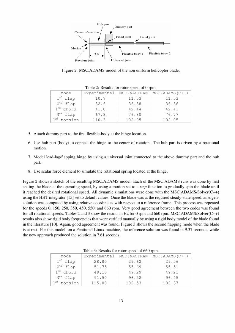
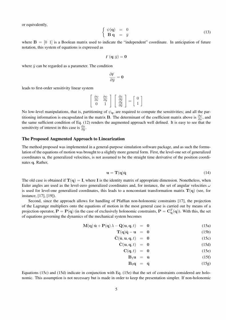
Figure 2: MSC.ADAMS model of the non uniform helicopter blade.
Table 2: Results for rotor speed of 0 rpm.Mode Experimental MSC.NASTRAN MSC.ADAMS(C++)
1st flap 10.7 11.53 11.532nd flap 32.6 36.38 36.361st chord 41.0 42.44 42.413rd flap 67.8 76.80 76.77
1st torsion 110.3 102.05 102.05
5. Attach dummy part to the first flexible-body at the hinge location.
6. Use hub part (body) to connect the hinge to the center of rotation. The hub part is driven by a rotationalmotion.
7. Model lead-lag/flapping hinge by using a universal joint connected to the above dummy part and the hubpart.
8. Use scalar force element to simulate the rotational spring located at the hinge.
Figure 2 shows a sketch of the resulting MSC.ADAMS model. Each of the MSC.ADAMS runs was done by firstsetting the blade at the operating speed, by using a motion set to a step function to gradually spin the blade untilit reached the desired rotational speed. All dynamic simulations were done with the MSC.ADAMS/Solver(C++)using the HHT integrator [15] set to default values. Once the blade was at the required steady-state speed, an eigen-solution was computed by using relative coordinates with respect to a reference frame. This process was repeatedfor the speeds 0, 150, 250, 350, 450, 550, and 660 rpm. Very good agreement between the two codes was foundfor all rotational speeds. Tables 2 and 3 show the results in Hz for 0 rpm and 660 rpm. MSC.ADAMS/Solver(C++)results also show rigid body frequencies that were verified manually by using a rigid body model of the blade foundin the literature [10]. Again, good agreement was found. Figure 3 shows the second flapping mode when the bladeis at rest. For this model, on a Pentium4 Linux machine, the reference solution was found in 9.37 seconds, whilethe new approach produced the solution in 7.61 seconds.
Table 3: Results for rotor speed of 660 rpm.Mode Experimental MSC.NASTRAN MSC.ADAMS(C++)
1st flap 28.80 29.62 29.562nd flap 51.75 55.69 55.511st chord 49.10 49.29 49.213rd flap 91.50 96.52 96.45
1st torsion 115.00 102.53 102.37
13
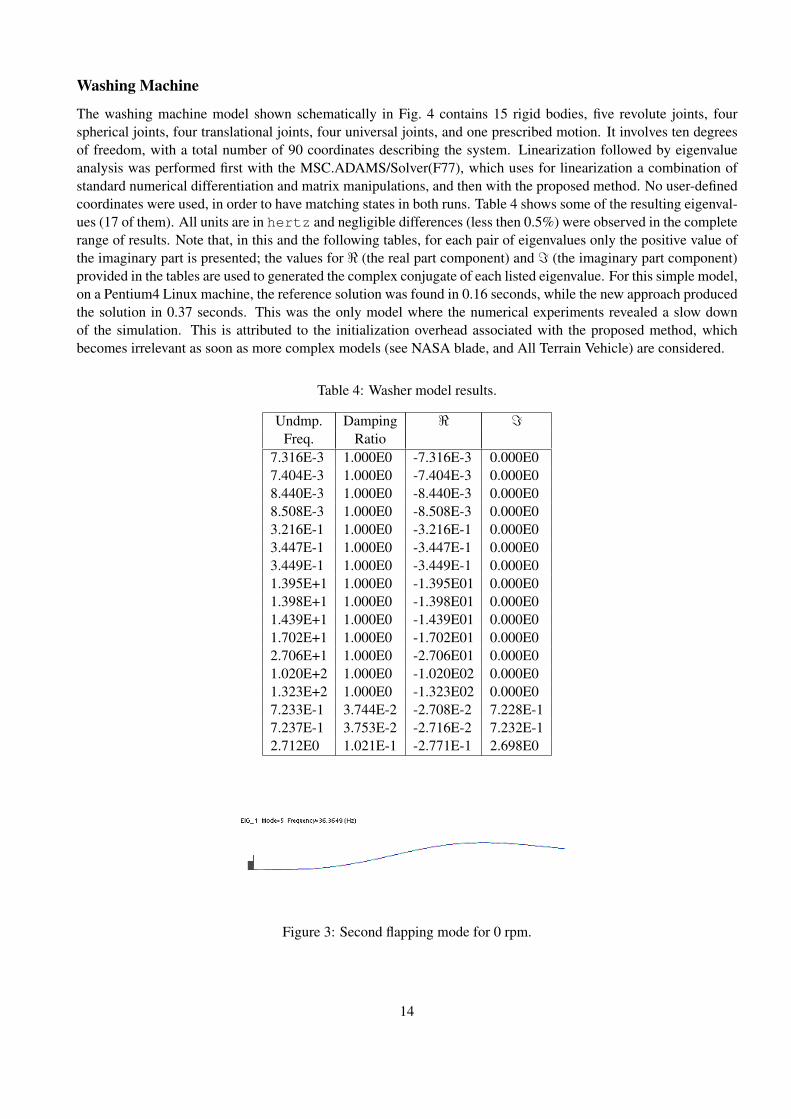
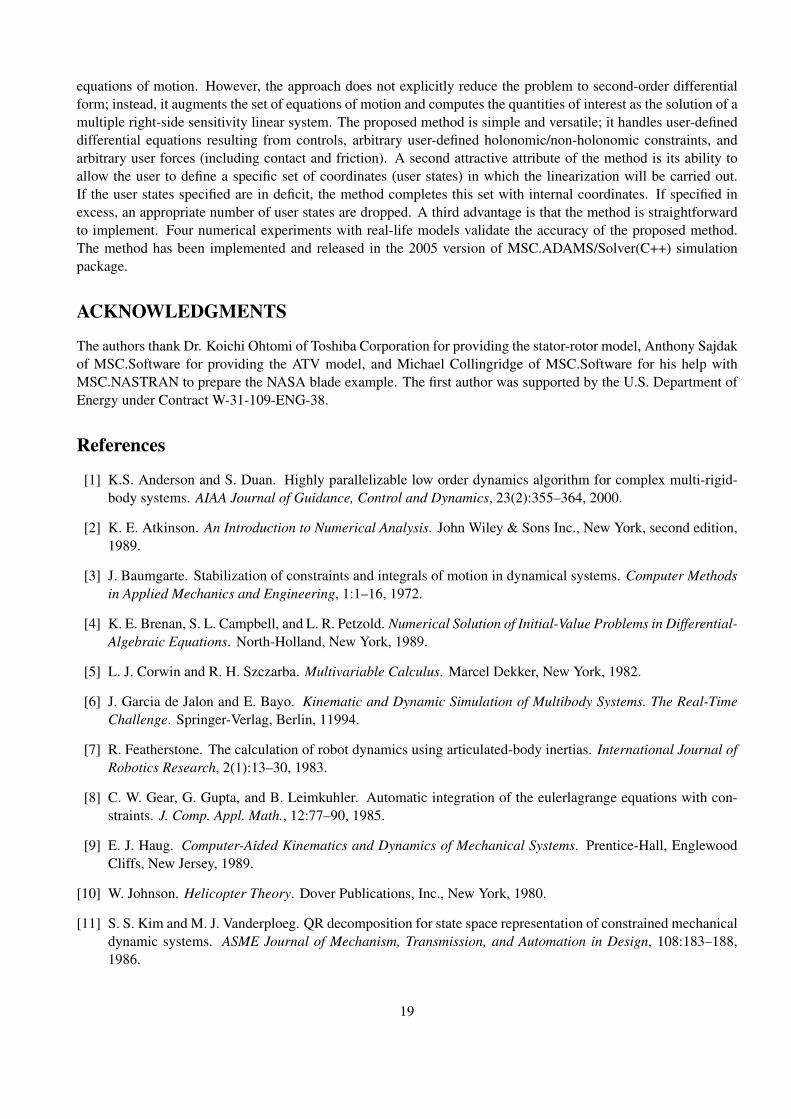
Washing Machine
The washing machine model shown schematically in Fig. 4 contains 15 rigid bodies, five revolute joints, fourspherical joints, four translational joints, four universal joints, and one prescribed motion. It involves ten degreesof freedom, with a total number of 90 coordinates describing the system. Linearization followed by eigenvalueanalysis was performed first with the MSC.ADAMS/Solver(F77), which uses for linearization a combination ofstandard numerical differentiation and matrix manipulations, and then with the proposed method. No user-definedcoordinates were used, in order to have matching states in both runs. Table 4 shows some of the resulting eigenval-ues (17 of them). All units are in hertz and negligible differences (less then 0.5%) were observed in the completerange of results. Note that, in this and the following tables, for each pair of eigenvalues only the positive value ofthe imaginary part is presented; the values for < (the real part component) and = (the imaginary part component)provided in the tables are used to generated the complex conjugate of each listed eigenvalue. For this simple model,on a Pentium4 Linux machine, the reference solution was found in 0.16 seconds, while the new approach producedthe solution in 0.37 seconds. This was the only model where the numerical experiments revealed a slow downof the simulation. This is attributed to the initialization overhead associated with the proposed method, whichbecomes irrelevant as soon as more complex models (see NASA blade, and All Terrain Vehicle) are considered.
Table 4: Washer model results.
Undmp. Damping < =Freq. Ratio
7.316E-3 1.000E0 -7.316E-3 0.000E07.404E-3 1.000E0 -7.404E-3 0.000E08.440E-3 1.000E0 -8.440E-3 0.000E08.508E-3 1.000E0 -8.508E-3 0.000E03.216E-1 1.000E0 -3.216E-1 0.000E03.447E-1 1.000E0 -3.447E-1 0.000E03.449E-1 1.000E0 -3.449E-1 0.000E01.395E+1 1.000E0 -1.395E01 0.000E01.398E+1 1.000E0 -1.398E01 0.000E01.439E+1 1.000E0 -1.439E01 0.000E01.702E+1 1.000E0 -1.702E01 0.000E02.706E+1 1.000E0 -2.706E01 0.000E01.020E+2 1.000E0 -1.020E02 0.000E01.323E+2 1.000E0 -1.323E02 0.000E07.233E-1 3.744E-2 -2.708E-2 7.228E-17.237E-1 3.753E-2 -2.716E-2 7.232E-12.712E0 1.021E-1 -2.771E-1 2.698E0
Figure 3: Second flapping mode for 0 rpm.
14

Figure 4: A washing machine example.
Figure 5: All terrain vehicle (ATV).
All Terrain Vehicle (ATV)
The ATV model presented in Fig. 5 has 28 rigid bodies, one flexible body, one cylindrical joint, three revolutejoints, 21 spherical joints, seven translational joints, four universal joints, six fixed joints, one inline primitive,five prescribed motions, 132 degrees of freedom, and a total of 314 coordinates describing the system (140 modalcoordinates were used to model the flexible body).
While the reference MSC.ADAMS/Solver(F77) and proposed MSC.ADAMS/Solver(C++) methods almostalways produce similar results, this is not always true. The results in Table 5 agree well, with the exception oftwo sets of eigenvalues. The source of these differences is a series of simplifying assumptions embedded in theprevious MSC.ADAMS solver and, to a lesser degree, the fact that the linearization was performed at the endof a dynamic simulation. The dynamic simulation was carried out with the legacy MSC.ADAMS/Solver(F77) inone case and with the new MSC.ADAMS/Solver(C++) in the other case. Given the complexity of the model, thesystem configuration at the end of the dynamic analysis is slightly different in the two solvers, and this contributesto the difference between the two sets of eigenvalues. Nonetheless, in the high-frequency range good agreementis observed between the reference (F77) and new (C++) implementations. For this model, on a Pentium4 Linuxmachine, the reference solution was found in 4.78 seconds, while the new approach produced the solution in 3.76seconds.
15

Table 5: ATV eigensolution for selected values. Proposed method results and % error.
< = ERR-<[%] ERR-=[%]-1.426E0 5.145E1 17.80 1.13-1.244E0 6.331E1 21.98 2.78-4.272E1 3.966E2 0.20 0.00-4.915E1 4.236E2 1.11 0.80-8.835E2 1.083E3 0.86 0.04-6.279E3 2.265E3 0.08 0.09-6.279E3 2.266E3 0.00 0.06-3.827E3 3.234E3 0.05 0.15-4.338E3 4.221E3 0.04 0.04-8.848E3 5.021E3 0.00 0.06
Figure 6: A Rotor-stator model.
Rotor-stator Model
Figure (6) shows a rotor-stator model for which a linearization of the equations of motion was carried out, followedby an eignesolution computation. The rotor is connected to the stator by a revolute joint with no friction and nocompliance elements between them. The stator is connected to the base by a bushing element, and the base isfixed to the ground. The physical properties of the rotor are m = 1300 kg, Ix = Iy = 500 kg m2, and Iz =1000 kg m2; and the center of mass is located at 0.75 m above the origin. The stator properties are m = 200 kg,Ix = Iy = 50 kg m2, and Iz = 10 kg m2. The bushing has translational constant K = 1000 N/m and C = 1 Ns/min all directions; the rotational constants about the x and y axes are Kt = 10000 N m and Ct = 10 N m s, and therotational constants about the z axis are Kt = 100000 N m and Ct = 100 N m s. The model has seven degreesof freedom and was linearized for different values of the initial angular speed of the rotor. The angular speed ofthe rotor has a big influence on the eigenvalues of the system. Moreover, given that the eigenvalues depend on thechoice of coordinates, two reference frames were selected to first linearize and then compute the eigensolutions.
The first choice was MARKER/4 (global reference) located on the base element. Results are shown inFig. (7)(a) for initial angular speeds of 0 Hz to 1 Hz. Notice that the plot shows only five eigenvalues of in-terest. Modes 5 and 6 correspond to the backward and forward rocking modes, respectively, while modes 2, 3,
16

Figure 7: Eigenvalues for speeds 0 Hz to 1 Hz. Global (a) and local (b) reference frames.
and 4 correspond to the translational modes. One mode has zero frequency (because of the free revolute joint),and another frequency corresponds to the rotation about a vertical axis (not shown for clarity). The second choicewas MARKER/1 (local reference), located on the rotor. Figure (7)(b) shows the corresponding results. Mode 5corresponds to the forward rocking mode, mode 6 corresponds to the backward rocking mode, and modes 2 and 3correspond to the horizontal translational modes.
A numerical experiment was set up to verify the results, as shown in Fig. (8). The base element is nowconnected to the ground by a motion constraint that imposes a random vibration. A second motion constraintwas added to the revolute joint to speed the rotor with an angular speed of f(t) = 0.0005(2πt). Also, a smallmass (0.001 kg) was attached to the rotor in order to create an eccentric excitation. A dynamic simulation wasundertaken from t = 0 to t = 2500 (the final prescribed speed of the rotor was 1.25 Hz), and the signals shownin Fig. 8 were collected and processed with an FFT filter. Figure (9)(a) shows the frequency content of signalDX(2,4) (the distance between markers 2 and 4). Notice the excellent match with the global computation shownin Fig. (7)(a).
Figure (9)(b) shows the frequency content of signal AY(4,1) (the small angle rotation of marker 1 aboutmarker 4). Notice the excellent match with the frequencies shown in Fig. (7)(b). The FFT plot of signal AY(4,1)highlights the rocking frequencies; to highlight the translational frequencies, the FFT plot of signal DX(4,1,1)(the distance between markers 1 and 4, measured in the reference frame associated with marker 1), shown inFig. (9)(c) was also generated. This numerical experiment validates the proposed linearization implemented inMSC.ADAMS/Solver(C++) and shows that the eigenvalues of a nonlinear system depend on the choice of coordi-nates used to linearized the system.
CONCLUSIONS
This paper presents a practical approach for computing at an operating point the linearization of the index 3 DAEsassociated with the time evolution of a constrained mechanical system. The method proposed is equivalent to astate-space reduction followed by linearization of the resulting set of second-order state space ordinary differential
17

Figure 8: Rotor-stator model setup for numerical experiment.
Figure 9: FFT plots of signals (a) DX(2,4), (b) AY(4,1), and (c) DX(4,1,1).
18
equations of motion. However, the approach does not explicitly reduce the problem to second-order differentialform; instead, it augments the set of equations of motion and computes the quantities of interest as the solution of amultiple right-side sensitivity linear system. The proposed method is simple and versatile; it handles user-defineddifferential equations resulting from controls, arbitrary user-defined holonomic/non-holonomic constraints, andarbitrary user forces (including contact and friction). A second attractive attribute of the method is its ability toallow the user to define a specific set of coordinates (user states) in which the linearization will be carried out.If the user states specified are in deficit, the method completes this set with internal coordinates. If specified inexcess, an appropriate number of user states are dropped. A third advantage is that the method is straightforwardto implement. Four numerical experiments with real-life models validate the accuracy of the proposed method.The method has been implemented and released in the 2005 version of MSC.ADAMS/Solver(C++) simulationpackage.
ACKNOWLEDGMENTS
The authors thank Dr. Koichi Ohtomi of Toshiba Corporation for providing the stator-rotor model, Anthony Sajdakof MSC.Software for providing the ATV model, and Michael Collingridge of MSC.Software for his help withMSC.NASTRAN to prepare the NASA blade example. The first author was supported by the U.S. Department ofEnergy under Contract W-31-109-ENG-38.
References
[1] K.S. Anderson and S. Duan. Highly parallelizable low order dynamics algorithm for complex multi-rigid-body systems. AIAA Journal of Guidance, Control and Dynamics, 23(2):355–364, 2000.
[2] K. E. Atkinson. An Introduction to Numerical Analysis. John Wiley & Sons Inc., New York, second edition,1989.
[3] J. Baumgarte. Stabilization of constraints and integrals of motion in dynamical systems. Computer Methodsin Applied Mechanics and Engineering, 1:1–16, 1972.
[4] K. E. Brenan, S. L. Campbell, and L. R. Petzold. Numerical Solution of Initial-Value Problems in Differential-Algebraic Equations. North-Holland, New York, 1989.
[5] L. J. Corwin and R. H. Szczarba. Multivariable Calculus. Marcel Dekker, New York, 1982.
[6] J. Garcia de Jalon and E. Bayo. Kinematic and Dynamic Simulation of Multibody Systems. The Real-TimeChallenge. Springer-Verlag, Berlin, 11994.
[7] R. Featherstone. The calculation of robot dynamics using articulated-body inertias. International Journal ofRobotics Research, 2(1):13–30, 1983.
[8] C. W. Gear, G. Gupta, and B. Leimkuhler. Automatic integration of the eulerlagrange equations with con-straints. J. Comp. Appl. Math., 12:77–90, 1985.
[9] E. J. Haug. Computer-Aided Kinematics and Dynamics of Mechanical Systems. Prentice-Hall, EnglewoodCliffs, New Jersey, 1989.
[10] W. Johnson. Helicopter Theory. Dover Publications, Inc., New York, 1980.
[11] S. S. Kim and M. J. Vanderploeg. QR decomposition for state space representation of constrained mechanicaldynamic systems. ASME Journal of Mechanism, Transmission, and Automation in Design, 108:183–188,1986.
19
[12] C. D. Liang and G. M. Lance. A differentiable null-space method for constrained dynamic analysis. ASMEJournal of Mechanism, Transmission, and Automation in Design, 109:405–410, 1987.
[13] MSCsoftware. ADAMS User Manual. Also available online at http://www.mscsoftware.com, 2005.
[14] MSC.Software. Nastran User Manual. Also available online at http://www.mscsoftware.com, 2005.
[15] D. Negrut, R. Rampalli, G. Ottarsson, and A. Sajdak. On the use of the HHT method in the context of index3 Differential Algebraic Equations of Multibody Dynamics. International Journal for Numerical Methods inEngineering, submitted, 2005.
[16] N. Orlandea, M. A. Chace, and D. A. Calahan. A sparsity-oriented approach to the dynamic analysis anddesign of mechanical systems – part I. Transactions of the ASME Journal of Engineering for Industry, pages773–779, 1977.
[17] L. A. Pars. A Treatise on Analytical Dynamics. John Wiley & Sons, New York, 1965.
[18] F. A. Potra. Implementation of linear multistep methods for solving constrained equations of motion. SIAM.Numer. Anal., 30(3), 1993.
[19] A. A. Shabana. Dynamics of Multibody Systems. Cambridge University Press, second edition, 1998.
[20] V. N. Sohoni and J. Whitesell. Automatic linearization of constrained dynamical models. ASME Journal ofMechanisms, Transmissions and Automation in Design, 108(8):300–304, 1986.
[21] R. A. Wehage and E. J. Haug. Generalized coordinate partitioning for dimension reduction in analysis ofconstrained dynamic systems. J. Mech. Design, 104:247–255, 1982.
[22] W.K. Wilkie, P.H. Mirick, and C.W. Langston. Rotating shake test and modal analysis of a model helicopterrotor blade. Computing Science Technical Report NASA Technical Memorandum 4760, Vehicle TechnologyCenter, U.S. Army Research Laboratory, Langley Research Center, Hampton, Virginia, 1997.
20