a practical and systematic review of weibull statistics
TRANSCRIPT

d e n t a l m a t e r i a l s 2 6 ( 2 0 1 0 ) 135–147
avai lab le at www.sc iencedi rec t .com
journa l homepage: www. int l .e lsev ierhea l th .com/ journa ls /dema
Review
A practical and systematic review of Weibull statistics forreporting strengths of dental materials
Janet B. Quinn, George D. Quinn ∗
ADAF Paffenbarger Research Center, National Institute of Standards and Technology, Gaithersburg, MD, USA
a r t i c l e i n f o
Article history:
Received 24 July 2009
Received in revised form
9 September 2009
Accepted 11 September 2009
Keywords:
Weibull
Review
Weibull standards
Flaw population
Extreme value distribution
Strength distribution
Characteristic strength
Strength comparison
Equivalent volume
Equivalent area
Alumina
Zirconia
Porcelain
Weibull modulus
a b s t r a c t
Objectives. To review the history, theory and current applications of Weibull analyses suffi-
cient to make informed decisions regarding practical use of the analysis in dental material
strength testing.
Data. References are made to examples in the engineering and dental literature, but this
paper also includes illustrative analyses of Weibull plots, fractographic interpretations, and
Weibull distribution parameters obtained for a dense alumina, two feldspathic porcelains,
and a zirconia.
Sources. Informational sources include Weibull’s original articles, later articles specific to
applications and theoretical foundations of Weibull analysis, texts on statistics and fracture
mechanics and the international standards literature.
Study selection. The chosen Weibull analyses are used to illustrate technique, the importance
of flaw size distributions, physical meaning of Weibull parameters and concepts of “equiva-
lent volumes” to compare measured strengths obtained from different test configurations.
Conclusions. Weibull analysis has a strong theoretical basis and can be of particular value
in dental applications, primarily because of test specimen size limitations and the use of
different test configurations. Also endemic to dental materials, however, is increased dif-
ficulty in satisfying application requirements, such as confirming fracture origin type and
diligence in obtaining quality strength data.
© 2009 Academy of Dental Materials. Published by Elsevier Ltd. All rights reserved.
Strength scaling
Maximum likelihood
Linear regression
∗ Corresponding author at: ADAF, Stop 854-6, National Institute of Standards and Technology, Gaithersburg, MD 20899, USA.Tel.: +1 301 975 5765.
E-mail address: [email protected] (G.D. Quinn).0109-5641/$ – see front matter © 2009 Academy of Dental Materials. Published by Elsevier Ltd. All rights reserved.doi:10.1016/j.dental.2009.09.006

136 d e n t a l m a t e r i a l s 2 6 ( 2 0 1 0 ) 135–147
Contents
1. Introduction . . . . . . . . . . . . . . . . . . . . . . . . . . . . . . . . . . . . . . . . . . . . . . . . . . . . . . . . . . . . . . . . . . . . . . . . . . . . . . . . . . . . . . . . . . . . . . . . . . . . . . . . . . . . . . . . . . 1361.1. Background: brittle failure prediction, fracture mechanics and flaws. . . . . . . . . . . . . . . . . . . . . . . . . . . . . . . . . . . . . . . . . . . . . . 1361.2. Extreme value distributions of “largest flaws” . . . . . . . . . . . . . . . . . . . . . . . . . . . . . . . . . . . . . . . . . . . . . . . . . . . . . . . . . . . . . . . . . . . . . . . 1371.3. The Weibull distribution . . . . . . . . . . . . . . . . . . . . . . . . . . . . . . . . . . . . . . . . . . . . . . . . . . . . . . . . . . . . . . . . . . . . . . . . . . . . . . . . . . . . . . . . . . . . . . 137
2. Considerations for using Weibull statistics for dental materials . . . . . . . . . . . . . . . . . . . . . . . . . . . . . . . . . . . . . . . . . . . . . . . . . . . . . . . . . . 1393. Experimental examples and discussion . . . . . . . . . . . . . . . . . . . . . . . . . . . . . . . . . . . . . . . . . . . . . . . . . . . . . . . . . . . . . . . . . . . . . . . . . . . . . . . . . . . . 140
3.1. Example 1: alumina 3- and 4-point flexure tests . . . . . . . . . . . . . . . . . . . . . . . . . . . . . . . . . . . . . . . . . . . . . . . . . . . . . . . . . . . . . . . . . . . . 1413.2. 3-Point and 4-point flexural strength comparisons using equivalent volumes . . . . . . . . . . . . . . . . . . . . . . . . . . . . . . . . . . . . 1413.3. Example 2: comparison of two porcelains using different sized flexure bars . . . . . . . . . . . . . . . . . . . . . . . . . . . . . . . . . . . . . . 1423.4. Example 3: Deviations from a unimodal strength distribution in a zirconia . . . . . . . . . . . . . . . . . . . . . . . . . . . . . . . . . . . . . . . 1433.5. Additional considerations and assumptions . . . . . . . . . . . . . . . . . . . . . . . . . . . . . . . . . . . . . . . . . . . . . . . . . . . . . . . . . . . . . . . . . . . . . . . . 143
4. Conclusion. . . . . . . . . . . . . . . . . . . . . . . . . . . . . . . . . . . . . . . . . . . . . . . . . . . . . . . . . . . . . . . . . . . . . . . . . . . . . . . . . . . . . . . . . . . . . . . . . . . . . . . . . . . . . . . . . . . . 144Acknowledgements . . . . . . . . . . . . . . . . . . . . . . . . . . . . . . . . . . . . . . . . . . . . . . . . . . . . . . . . . . . . . . . . . . . . . . . . . . . . . . . . . . . . . . . . . . . . . . . . . . . . . . . . . . 144Appendix A . . . . . . . . . . . . . . . . . . . . . . . . . . . . . . . . . . . . . . . . . . . . . . . . . . . . . . . . . . . . . . . . . . . . . . . . . . . . . . . . . . . . . . . . . . . . . . . . . . . . . . . . . . . . . . . . . . 144References . . . . . . . . . . . . . . . . . . . . . . . . . . . . . . . . . . . . . . . . . . . . . . . . . . . . . . . . . . . . . . . . . . . . . . . . . . . . . . . . . . . . . . . . . . . . . . . . . . . . . . . . . . . . . . . . . . . . 146
1. Introduction
This paper reviews Weibull statistics in order to facilitateinformed decisions regarding practical use of the analysis as itapplies to dental material strength testing. Weibull statisticsare commonly used in the engineering community, but to asomewhat lesser extent in the dental field where applicabilityhas been questioned [1,2]. A possible confusing factor is thatWaloddi Weibull originally presented his analyses partiallyon empirical grounds; published theoretical confirmation wasnot available until many years later. Even as a theoretical basiswas being constructed, Weibull, as an engineer, seemed moreconcerned with what worked [3,4]. In order to assess applica-bility to the specific field of dental material strength testing, itis helpful to start with a brief history and overview of basicconcepts of extreme value theory, fracture mechanics, andflaw populations as they pertain to the theoretical foundationof Weibull analysis.
1.1. Background: brittle failure prediction, fracturemechanics and flaws
It is often noted that dental restorative ceramics and compos-ites, while popular in terms of esthetics and biocompatibility,are susceptible to brittle fracture. This type of failure is partic-ularly difficult to predict. Imminent brittle fracture is seldompreceded by warning, such as visible deformation, nor doseemingly identical brittle components appear to break atthe same applied stress. Ductile materials deform to evenlydistribute stresses throughout a region, but in stiff, brit-tle materials, stress concentrations at specimen geometrychanges, cracks, surface irregularities, pores and other intrin-sic flaws are not relieved. Hence the design methodologies andtest methods for ductile materials are unsuitable for brittle
demonstrated the inapplicability of ductile strength testinganalyses to brittle failure prediction. Such disasters spurredthe development of the science of fracture mechanics in orderto understand the conditions of failure through crack growthrather than by ductile mechanisms [7].
In the early 1920s, Griffith postulated that crack exten-sion in brittle materials occurs when there is sufficient elasticstrain energy in the vicinity of a growing crack to form two newsurfaces [8]. In the 1950s Irwin built on Griffith’s work to asso-ciate crack extension with an “energy release rate” [9]. This ledto a new parameter, KIc—fracture toughness, or resistance tocrack growth. Irwin’s approach enabled strength predictionsbased on fracture toughness calculations that relate crackextension to the sizes of preexisting cracks or “flaws” withina material. For the most common case of a small flaw in a farfield tensile stress field, modern fracture mechanics relatesthe applied fracture stress at the fracture origin, �f, to a flawsize, c [7]:
�f = KIc
Y√
c(1)
where Y is a dimensionless, material-independent constant,related to the flaw shape, location and stress configurationand is called the stress intensity shape factor. “Flaws” are notnecessarily inadvertent defects or blemishes in a material. Nomaterial is perfectly homogenous, and all contain some sortof discontinuities on some scale. These discontinuities mightbe pores, inclusions, distributed microcracks associated withgrain boundaries or phase changes during processing, regionsof dislocations or slight variations of chemistry, or many otherpossible variants and combinations. They could also be sur-face distributed flaws such as grinding cracks. Flaws in thissense are intrinsic to the material or the way it was shaped
materials and different test methods and design approachesare needed.
A series of catastrophic events, often epitomized by the Lib-erty ship [5] and Comet airplane [6] disasters, spectacularly
or processed, and are distributed in some way throughout thematerial surface or volume. It can be seen from the equationthat the smallest strengths are associated with the largest flawsizes.
2 6
orsdamtswdtobta
1
Smtssepflw
sotenIwpm
s
FWpp(
d e n t a l m a t e r i a l s
The idea of failure being associated with a largest flaw,r “weakest link theory”, is not recent. Leonardo DaVinci iseputed to have conducted tests circa 1500 involving basketsuspended by different lengths of wire of nominally identicaliameter [10]. DaVinci gradually filled the baskets with sandnd noted the baskets suspended by shorter wires could holdore sand, an outcome that is expected if it is assumed that
here is a lower probability of encountering a large flaw in ahorter wire. DaVinci did not know exactly where a particularire would break, but he recommended that multiple tests beone for each wire length, suggesting that there was a statis-ical variation in the strengths and failure locations of wiresf a the same length. Since DaVinci’s time, much progress haseen made both in our ability to identify critical flaw proper-ies and in refining predictions based on weakest link theorynd statistical failure probabilities.
.2. Extreme value distributions of “largest flaws”
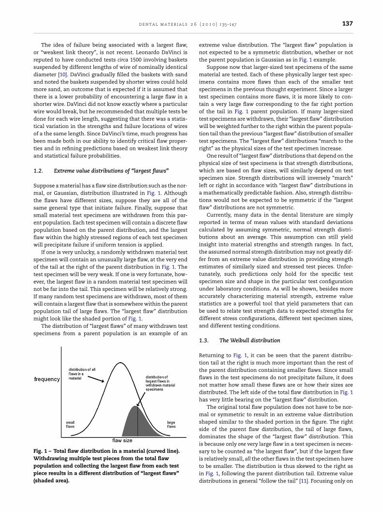
uppose a material has a flaw size distribution such as the nor-al, or Gaussian, distribution illustrated in Fig. 1. Although
he flaws have different sizes, suppose they are all of theame general type that initiate failure. Finally, suppose thatmall material test specimens are withdrawn from this par-nt population. Each test specimen will contain a discrete flawopulation based on the parent distribution, and the largestaw within the highly stressed regions of each test specimenill precipitate failure if uniform tension is applied.
If one is very unlucky, a randomly withdrawn material testpecimen will contain an unusually large flaw, at the very endf the tail at the right of the parent distribution in Fig. 1. Theest specimen will be very weak. If one is very fortunate, how-ver, the largest flaw in a random material test specimen willot be far into the tail. This specimen will be relatively strong.
f many random test specimens are withdrawn, most of themill contain a largest flaw that is somewhere within the parent
opulation tail of large flaws. The “largest flaw” distributionight look like the shaded portion of Fig. 1.The distribution of “largest flaws” of many withdrawn testpecimens from a parent population is an example of an
ig. 1 – Total flaw distribution in a material (curved line).ithdrawing multiple test pieces from the total flaw
opulation and collecting the largest flaw from each testiece results in a different distribution of “largest flaws”
shaded area).
( 2 0 1 0 ) 135–147 137
extreme value distribution. The “largest flaw” population isnot expected to be a symmetric distribution, whether or notthe parent population is Gaussian as in Fig. 1 example.
Suppose now that larger-sized test specimens of the samematerial are tested. Each of these physically larger test spec-imens contains more flaws than each of the smaller testspecimens in the previous thought experiment. Since a largertest specimen contains more flaws, it is more likely to con-tain a very large flaw corresponding to the far right portionof the tail in Fig. 1 parent population. If many larger-sizedtest specimens are withdrawn, their “largest flaw” distributionwill be weighted further to the right within the parent popula-tion tail than the previous “largest flaw” distribution of smallertest specimens. The “largest flaw” distributions “march to theright” as the physical sizes of the test specimen increase.
One result of “largest flaw” distributions that depend on thephysical size of test specimens is that strength distributions,which are based on flaw sizes, will similarly depend on testspecimen size. Strength distributions will inversely “march”left or right in accordance with “largest flaw” distributions ina mathematically predictable fashion. Also, strength distribu-tions would not be expected to be symmetric if the “largestflaw” distributions are not symmetric.
Currently, many data in the dental literature are simplyreported in terms of mean values with standard deviationscalculated by assuming symmetric, normal strength distri-butions about an average. This assumption can still yieldinsight into material strengths and strength ranges. In fact,the assumed normal strength distribution may not greatly dif-fer from an extreme value distribution in providing strengthestimates of similarly sized and stressed test pieces. Unfor-tunately, such predictions only hold for the specific testspecimen size and shape in the particular test configurationunder laboratory conditions. As will be shown, besides moreaccurately characterizing material strength, extreme valuestatistics are a powerful tool that yield parameters that canbe used to relate test strength data to expected strengths fordifferent stress configurations, different test specimen sizes,and different testing conditions.
1.3. The Weibull distribution
Returning to Fig. 1, it can be seen that the parent distribu-tion tail at the right is much more important than the rest ofthe parent distribution containing smaller flaws. Since smallflaws in the test specimens do not precipitate failure, it doesnot matter how small these flaws are or how their sizes aredistributed. The left side of the total flaw distribution in Fig. 1has very little bearing on the “largest flaw” distribution.
The original total flaw population does not have to be nor-mal or symmetric to result in an extreme value distributionshaped similar to the shaded portion in the figure. The rightside of the parent flaw distribution, the tail of large flaws,dominates the shape of the “largest flaw” distribution. Thisis because only one very large flaw in a test specimen is neces-sary to be counted as “the largest flaw”, but if the largest flaw
is relatively small, all the other flaws in the test specimen haveto be smaller. The distribution is thus skewed to the right asin Fig. 1, following the parent distribution tail. Extreme valuedistributions in general “follow the tail” [11]. Focusing only on
l s 2
138 d e n t a l m a t e r i athe tails allows simple, generalized parametric functions to beused in extreme value statistical models. Such models havebeen defined to accommodate underlying distribution tailsthat deviate considerably from the Gaussian shape in Fig. 1example.
There are three commonly recognized families of extremevalue distributions [11–13] where G(x) is the probability distri-butions function for an outcome being less than x for a sampleset of n independent measurements:
Type I. Gumbel G(x) = exp(−exp−(x−�)/� ) for all x
Type II. Fréchet : G(x)
{= exp(−((x − �)/�)−�) for x ≥ �
= 0 otherwise
Type III. Weibull : G(x)
{= exp(−((� − x)/�)�) for x ≤ �
= 1 otherwise
where �, �(>0), and �(>0) are the location, scale and shapeparameters, respectively.
Fisher and Tippet [12] are credited [11,13] with defining theextreme value distributions in 1928, when they showed therecould only be the three types. Some graphical examples ofthe probability density functions of the three types of extremevalue distributions are shown in Fig. 2.
All three extreme value distributions have a theoreticalbasis for characterizing phenomena founded on weakest linktheory. For strength dependency on an underlying materialflaw distribution, the goodness-of-fit of any of the extremevalue distributions depends on the shape of the flaw distribu-tion tail. In this regard, Type III, or the Weibull distribution, isusually considered the best choice because it is bounded (thelowest possible fracture strength is zero), the parameters allowcomparatively greater shape flexibility, it can provide reason-ably accurate failure forecasts with small numbers of test
specimens and it provides a simple and useful graphical plot[4,14]. In what has been hailed as his “hallmark paper” in 1951[15], Weibull based the wide applicability of the distribution onfunctional simplicity, satisfaction of necessary boundary con-Fig. 2 – Probability density functions for the three extremevalue distributions, arbitrarily placed along the abscissa (x)axis for easier shape comparison. Both the Weibull andGumbel functions have demonstrated good fits forstrengths of brittle materials, but a theoretical basis hasbeen demonstrated for the Weibull distribution.
6 ( 2 0 1 0 ) 135–147
ditions and, mostly, good empirical fit. The parameter symbolsand form of the extreme value functions are usually writ-ten differently for reliability analyses. In the specific case ofWeibull fracture strength analysis, the cumulative probabil-ity function is written such that the probability of failure, Pf,increases with the fracture stress variable, �:
Pf = 1 − exp[−(
� − �u
��
)m](2)
This is known as the Weibull three parameter strength dis-tribution. The threshold stress parameter, �u, represents aminimum stress below which a test specimen will not break.The scale parameter or characteristic strength, �� , is depen-dent on the stress configuration and test specimen size.The distribution shape parameter, m, is the Weibull modu-lus. This is the equation form that Weibull presented in hisoriginal publications, directly derived from weakest link the-ory [3]. He was conservative and disclaimed any theoreticalbasis, not because of misgivings concerning extreme value orweakest link theory, which was well established by then, butbecause he perceived it was “hopeless to expect a theoreti-cal basis for distribution functions of random variables suchas strength properties”. Since Weibull’s initial publications in1939 and 1951, however, the science of fracture mechanicshas enabled determinations of quantitative functional rela-tionships between strength and flaws in brittle materials, asexemplified in Eq. (1).
By 1977, Jayatilaka and Trustrum [16] used fracturemechanics to develop a general expression for the failureprobability using several general flaw size distributions sug-gested by experimental work. They coupled these flaw sizedistributions with the fracture mechanics criterion, Eq. (1),and integrated the risk of breakage over component volumesand then derived a number of different strength distributions[16,17]. Their derivations are too lengthy to repeat here and thereader is encouraged to review their exposition in the originalreferences. They showed that the right side tail of many par-ent flaw size distributions such as shown in Fig. 1 often canbe modeled by a simple power law function: f(c) = constant c−n
where c is the flaw size. In such cases, the resulting strengthdistribution is the Weibull distribution with m = 2n − 2. Danzeret al. [18–20] have done similar derivations with more gen-eralized flaw size distributions and have reached the sameconclusions. Subsequent work, including painstaking mea-surement of flaw sizes and constructing distributions, hasconfirmed the power law function for the distribution of largecrack sizes and hence the theoretical basis for the Weibullapproach [21–23]. In other words, a reasonable power lawdistribution for large flaw sizes, classical fracture mechanicsanalysis, and weakest link theory lead directly to the Weibullstrength distribution.
Today’s engineers routinely utilize Weibull statistics forcharacterizing failure of brittle materials. Numerous anddiverse studies in the engineering literature report data interms of Weibull parameters where the strengths are related
to fractographically determined flaw types and sizes [24–26].Such studies substantiate the existence of flaw distributionsthat lead to strength distributions that can be modeled byWeibull statistics for a wide range of materials. As noted ear-
2 6
litflprdut
ptJt[2tWfua
iasa
2s
AntdTdssistfscmtipW
flAflfsmtom
d e n t a l m a t e r i a l s
ier, fractographic examinations are becoming more commonn relating flaw types and sizes to strengths of dental restora-ion materials [27–29]. While this shows that characterizingaw populations in dental materials is possible, this does notrove it is easy or possible in every case. Many dental mate-ials have rough microstructures, where it can be particularlyifficult to identify fractographic features [30,31]. Also, it is notnusual to have multiple flaw types present which complicatehe Weibull analysis.
Major standards organizations throughout the world haveublished specific guidelines for reporting ceramic strength inerms of Weibull parameters, including ASTM (C1239) [32], theapanese Industrial Standards Organization (JIS R1625) [33],he European Committee for Standardization (CEN ENV 843)34], and the International Organization for Standards (ISO0501) [35]. These standards are very similar and use the iden-ical Maximum Likelihood Estimation analysis to calculate the
eibull parameters. A newly revised (2008) Ceramic Materialor Dentistry standard (ISO 6872) [36] is the sole exception andses a simpler linear regression calculation in an informativennex.
Since many brittle materials used in structural engineer-ng are also used in restorative dentistry, are Weibull analysesppropriate for ceramic dental materials? To answer this, thepecific underlying assumptions and conditions inherent inpplying Weibull statistics must be examined.
. Considerations for using Weibulltatistics for dental materials
good data set is required for any credible property determi-ation, and it can be deduced from the previous paragraphshat diligence in test specimen preparation and testing proce-ures is particularly important when using Weibull statistics.est specimens breaking from inconsistent machining or han-ling, or haphazard alignment, are not representative of apecific flaw population, and do not contribute to a valid dataet for Weibull analysis. A materials advisory board committeen 1980 [37] concluded that: “Ceramic strength data must meettringent quality demands if they are to be used to determinehe failure probability of a stressed component. Statisticalracture theory is based on the premise that specimen-to-pecimen variability of strength is an intrinsic property of theeramic, reflecting its flaw population and not unassignableeasurement errors. Ceramic strength data must be essen-
ially free of experimental error.” Even with meticulous testmplementation, however, it is the stipulation of a single flawopulation that seems to cause the most difficulty in usingeibull statistics in dental material strength testing.In Eq. (1), the parameter Y distinguishes different types of
aws as well as different test specimen test configurations.blunt flaw, such as a pore, is more benign than a sharp
aw, such as a microcrack. A material under load may breakrom a sharp flaw but not break from a blunt flaw of a similarize. Suppose a material contains the two flaw types, small
icrocracks and large pores. Each flaw type has its own dis-ribution. If all the test specimens break from microcracks,r all the test specimens break from pores, then either theicrocrack size distribution or the pore size distribution will
( 2 0 1 0 ) 135–147 139
govern the strength distribution. If, however, some test speci-mens break from microcracks, and other test specimens breakfrom pores, the strength distributions resulting from the dif-ferent flaw populations overlap and an associated extremevalue distribution cannot be modeled by one single flaw sizedistribution tail. In this case, the Weibull strength distribu-tion would not be expected to appear smoothly continuous.If many test specimens are tested and enough of them breakfrom either flaw population, parts of two distinct Weibull dis-tributions may be discernable. Censored statistical analysesmust be used in such cases [32]. Bends or kinks in a Weibulldistribution function are often indicative of fracture resultingfrom multiple flaw types.
Thus, lack of a good Weibull fit is suggestive of an inconsis-tent underlying flaw population, assuming the material wastested properly and failed in a brittle manner. Conversely, agood Weibull fit is sometimes taken as indicative of a sin-gle, dominant flaw type and confirmation of adequate carein testing procedures. Unless material familiarity and previ-ous testing dictates otherwise, it is prudent to verify the causeof fracture initiation. This is often done fractographically andis encouraged, and in cases required, by the standards forWeibull analyses [32–35]. There even are guidelines and formalstandards for fractographic analysis that have been preparedwith Weibull analysis in mind [31,38].
Another consideration in using Weibull statistics is theincreased number of test specimens that might be needed tocharacterize an entire strength distribution rather than sim-ply estimate a mean strength value. The optimal number oftest specimens depends on many variables, including mate-rial and testing costs, the values of the distribution parametersand the desired precision for an intended application. Help-ful calculations and tables to make such decisions can befound in the previously cited standards. In the absence ofspecific requirements, a general rule-of-thumb is that approx-imately 30 test specimens provide adequate Weibull strengthdistribution parameters, with more test specimens contribut-ing little towards better uncertainty estimates [39–41]. Moreinformation regarding optimal test specimen numbers, as wellas reasons why Weibull distributions are so often observedin material testing practice are discussed by Danzer et al.[19]. They also detail conditions necessary to obtain a Weibulldistribution and suggest alternative statistical approachesfor analyzing strength data for materials that do not satisfythese conditions, such as materials with unusual or highlymixed flaw distributions. In this sense, Weibull analysis canbe regarded as a special, simple case of a broader statisticalapproach for analyzing strength data [18–20]. Indeed, Danzernow uses the expression “Weibull material” as one with a sin-gle flaw type whose size distribution fits a power law functionon the right side tail.
The previous paragraphs highlight some of the assump-tions and difficulties in utilizing Weibull statistics incharacterizing strength measurements of dental materials.What are the benefits?
It was initially noted that extreme value statistics can be
used to predict changes in distributions according to the phys-ical size of the individual test specimens. This is one of thestrongest virtues of the Weibull model and what distinguishesit from other distributions. In practical terms, this means that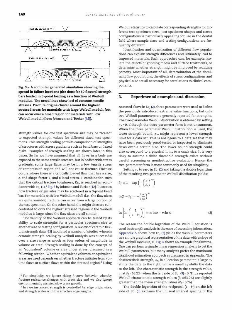
140 d e n t a l m a t e r i a l s 2
Fig. 3 – A computer generated simulation showing thespread in failure locations (the dots) for 50 flexural strengthbars loaded in 3-point loading as a function of Weibullmodulus. The arced lines show loci of constant tensilestresses. Fracture origins cluster around the higheststressed areas for materials with large Weibull moduli, but
can occur over a broad region for materials with lowWeibull moduli (from Johnson and Tucker [42]).strength values for one test specimen size may be “scaled”to expected strength values for different sized test speci-mens. This strength scaling permits comparison of strengthsof structures with stress gradients such as bend bars or flexeddisks. Examples of strength scaling are shown later in thispaper. So far we have assumed that all flaws in a body areexposed to the same tensile stresses, but in bodies with stressgradients, some large flaws may be in a low tensile stressor compression region and will not cause fracture. Fractureoccurs where there is a critically loaded flaw that has a size,c, and shape factor Y, and a local stress, �, combination suchthat the critical fracture toughness, KIc, is reached in accor-dance with eq. (1).1 Fig. 3 by Johnson and Tucker [42] illustrateshow fracture origin sites may be scattered in a 3-point bendbar. For materials with low Weibull moduli (i.e., the flaw sizesare quite variable) fracture can occur from a large portion ofthe test specimen. On the other hand, the origin sites are con-centrated to only the highest stressed regions if the Weibullmodulus is large, since the flaw sizes are all similar.
The validity of the Weibull approach can be tested by itsability to scale strengths for a particular specimen size toanother size or testing configuration. A review of ceramic flex-ural strength data [43] tabulated a number of studies whereinceramic strength scaling by Weibull analysis was successfulover a size range as much as four orders of magnitude involume or area! Strength scaling is done by the concept ofan “equivalent” volume or area under stress, discussed in a
following section. Whether equivalent volumes or equivalentareas are used depends on whether fracture initiates from vol-ume flaws or surface flaws within the stressed region.2 Using1 For simplicity, we ignore rising R-curve behavior wherebyfracture resistance changes with crack size and we also ignoreenvironmentally assisted slow crack growth.
2 In rare instances, strength is controlled by edge origin sites,and strength scales with the effective edge lengths.
6 ( 2 0 1 0 ) 135–147
Weibull statistics to calculate corresponding strengths for dif-ferent test specimen sizes, test specimen shapes and stressconfigurations is particularly appealing for use in the dentalfield where sample sizes and testing configurations are fre-quently different.
Identification and quantization of different flaw popula-tions can explain strength differences and ultimately lead toimproved materials. Such approaches can, for example, iso-late the effects of grinding media and surface treatments, ordetermine whether strength might be improved by reducingporosity. Most important of all, determination of the domi-nant flaw populations, the effects of stress configurations andphysical size are all necessary for correlations to clinical com-ponents.
3. Experimental examples and discussion
As noted above in Eq. (2), three parameters were used to definethe previously introduced extreme value functions, but onlytwo Weibull parameters are generally reported for strengths.The two-parameter Weibull distribution is obtained by setting�u = 0, although the three parameter form is not uncommon.When the three parameter Weibull distribution is used, thelower strength bound, �u, might represent a lower strengthlimit for a data set. This is analogous to a data set that mayhave been previously proof-tested or inspected to eliminateflaws over a certain size. The lower bound strength couldalso correspond to a physical limit to a crack size. It is veryrisky to assume a finite threshold strength exists withoutcareful screening or nondestructive evaluation. Hence, thetwo-parameter form is most commonly used for simplicity.
Setting �u to zero in Eq. (2) and taking the double logarithmof the resulting two-parameter Weibull distribution yields:
Pf = 1 − exp(
−(
�
��
)m)
ln(1 − Pf ) = −(
�
��
)m
ln
[ln
(1
1 − Pf
)]= m ln � − m ln �� (3)
The reason the double logarithm of the Weibull equation isused in strength analysis is the ease of accessing information.Appendix A shows how Eq. (3) yields the Weibull parametersin a simple graphical representation of the data with a slope ofthe Weibull modulus, m. Fig. 4 shows an example for alumina.One can perform a simple linear regression analysis to get theWeibull parameters, but many analysts prefer the maximumlikelihood estimation approach as discussed in Appendix. Thecharacteristic strength, �� , is a location parameter; a large ��
shifts the data to the right, while a small �� shifts the datato the left. The characteristic strength is the strength value,�, at P = 63.2%, when the left side of Eq. (3) = 0. Thus reported
fWeibull characteristic strength values (Pf = 63.2%) are slightlygreater than the mean strength values (Pf = 50%).
The double logarithm of the reciprocal (1 − Pf) on the leftside of Eq. (3) explains the unusual interval spacing of the

d e n t a l m a t e r i a l s 2 6
Fig. 4 – Weibull plots of alumina bars broken in flexureusing 3-point (�) and 4-point (©) test configurations. Thebars broken in 3-point flexure broke at greater stresses. Theparallel shift to the right of the whole distribution ispredicted by Weibull theory. The Weibull parameters andfi
Pect
3
Ttbtus
�
�
wt1to
wttv(d
flaw mix probably contributed to some of the wriggles in Fig. 4
tted lines are from maximum likelihood analysis.
f labels on the ordinate (y) axis of the Weibull graph. Twoxamples are used in this section to illustrate the previousoncepts. The example in Appendix A also illustrates some ofhese topics.
.1. Example 1: alumina 3- and 4-point flexure tests
his first example illustrates strength differences in polycrys-alline alumina bars tested in 3-point and 4-point flexure. Thear sizes were all 3 mm × 4 mm × 50 mm. The 3-point flexureest specimens had 40 mm outer spans, and the 4-point flex-re test specimens had 40 mm outer spans and 20 mm innerpans. Stresses were calculated by the formulae [44]:
3-pt = 3PL
2bd2for the 3-point flexure tests
4-pt = 3PL
4bd2for the 1/4-point, 4-point flexure configuration
here P is the break load, L is the outer span length, b is theest specimen width, and d is the test specimen height. The/4-point qualifier for the 4-point configuration means thathe inner loading rollers are located inward by 1/4L from theuter loading rollers.
For each of the two test configurations, the stress valuesere ranked in ascending order, i = 1, 2, 3, . . ., N, where N is the
otal number of test specimens and i is the ith datum. Thus,he lowest stress for each configuration represents the first
alue (i = 1), the next lowest stress value is the second datumi = 2), etc., and the highest stress is represented by the Nthatum. This enables a ranked probability of failure, Pf (�i), to( 2 0 1 0 ) 135–147 141
be assigned to each datum according to
Pf (�i) = i − 0.5N
(4)
Although there are other formulations to assign failure prob-abilities, the one shown in Eq. (4) is widely used and hasnegligible bias as discussed in Appendix.
Since the fracture stress and the associated Pf for eachdatum are now known, a graph may be constructed using theleft side of Eq. (3) on the ordinate and ln(�) on the abscissa. Thiscomprises Fig. 4, where the 3-point flexure bar data (squares)are at the right, at higher strengths, than the 4-point flexurebar data (circles). There are two common approaches to fit aline through the data: linear regression analysis and maxi-mum likelihood estimation analysis [45–48]. The pros and consof each analysis are described in more detail in the Appendix,but, as mentioned above, most world standards use the latter.The MLE analysis was used for the Weibull parameter esti-mates in Fig. 4 and Table 1. The strength difference for thesame material seems large, but this is to be expected accord-ing to weakest link theory, as more material is under higherstress in the 4-point configuration, with a higher probabilityof containing a larger flaw.
It can be seen from Fig. 4 that the slopes (Weibull moduli)indicate the strength distribution widths. The similar slopessuggest that the same flaw types were active in both specimensets and this indeed was verified by fractographic analysis.The wriggles in the curves are not unusual and are commonin small size sample sets. A high modulus, or steep slope, isassociated with a narrow strength distribution. This is usu-ally desirable, as materials with high Weibull moduli are morepredictable and less likely to break at a stress much lowerthan a mean value. The characteristic strength, or Weibullscale parameter �� , indicates the distribution location alongthe abscissa (x) axis, and is expected to move according totest specimen size or the amount of material that is highlystressed. Thus, the distributions for 3- and 4-point flexure areexpected to have the same shape (m value), but move to theright (higher �� value) as test specimen sizes or stressed vol-umes decrease. This is directly analogous to the “march” ofthe “largest flaw” distribution presented in a previous section.It was also stated in previous sections that such measuredstrength changes due to differences in test specimen size andconfiguration can be quantitatively predicted using Weibullparameters. This can be accomplished through the concept ofequivalent areas or volumes.
3.2. 3-Point and 4-point flexural strength comparisonsusing equivalent volumes
Fractographic analysis of the flexure test specimens graphedin Fig. 4 determined the predominant flaw type was volume-distributed porosity or agglomerates associated with porosity.Inclusions caused fracture in some test specimens, and the
data. Since the flaws were volume distributed, we will com-pare the two data sets using an equivalent volume approach.In the Weibull weakest link model, the size-strength relation-

142 d e n t a l m a t e r i a l s 2 6 ( 2 0 1 0 ) 135–147
Table 1 – Strength tests with different flexural configurations and maximum likelihood estimates of the Weibullparameters.
Material (numberof specimens)
Flexure test type Mean strength(std. dev.)
Weibull char. strength,�� (90% conf. interval)
Weibull modulus, m (90%conf. interval)
MPaMPa.3) MPa
Alumina (32) 4-point, 40 mm × 20 mm spans 364(45)Alumina (30) 3-point, 40 mm span 444(51)Porcelain 1 (27) 4-point, 20 mm × 40 mm spans 84.7 (5Porcelain 2 (26) 4-point, 10 mm × 20 mm spans 112(8) M
ship can be expressed [43,46–48]:
�1
�2=
(VE2
VE1
)1/m
(5)
where m is the Weibull modulus, �1 and �2 are the mean (ormedian or characteristic) strengths of test specimens of type 1and 2 which may have different sizes and stress distributions,and VE1 and VE2 are the associated effective volumes. (Effectiveareas may be substituted for the effective volumes in Eq. (5)for surface flaws, such as machining damage.) A unimodal flawpopulation that is uniformly distributed throughout the vol-ume and a Weibull two-parameter distribution are assumed.
The effective volume approach is illustrated in Fig. 5. In thesimplest case of direct uniform tension, VE is the test speci-men volume, V. Many test specimens or components such asflexural loaded rods or bars have stress gradients and VE < V.Sometimes the relationship between the two is expressed asVE = KV, where K is called the loading factor and is dimension-less and V is the total volume within the outer loading points.As shown in Fig. 5, VE is the volume of a hypothetical tensiletest specimen, which when subjected to the stress �max, has
the same probability of fracture as the flexure test specimenstressed at �max. In other words, a flexure bar of volume Vis equivalent to a tensile test specimen of size VE. K is 1 foran ideally loaded tension specimen. K is typically less than 1Fig. 5 – The concept of equivalent volume. �x shows thedirection of the tensile stresses. Only part of the totalvolume, V, of the flexure specimen on the left is in tension.Only a smaller fraction of this region (depicted by theshaded area) is exposed to large tension stresses. Anequivalent direct tension specimen with the same effectivevolume, VE, is shown on the right. How much of the flexurespecimen volume should be counted depends on theWeibull modulus.
383(370–396) MPa 9.6 (7.3–11.7)467(449–485) MPa 8.8 (6.6–10.7)
Pa 87.1 (85.4–88.8) MPa 18.5 (13.6–22.7)115(113–118) MPa 18.0 (13.1–22.2)
for parts or test specimens that have stress gradients, i.e., thestress varies with position within the body.
Equations for effective volumes and effective areas may bedetermined from knowledge of the stress state, or looked upin the literature for common configurations, such as flexure ofrectangular bars [49] or round rods [50]. For the flexure bars inFig. 4, the effective volumes can be calculated:
VE of the 1/4-point 4-point flexure test specimen
= (Lobd)(m + 2)
[4(m + 1)2]
VE of the 3-point flexure test specimens = (Lobd)
[2(m + 1)2]
where Lo is the outer span length, b is the test specimen width,d is the test specimen height, and m is the Weibull modulus.In other words, the effective volumes are equal to the spec-imen volume (Lobd) within the loading span multiplied by adimensionless term including the Weibull modulus. The latterterm takes into account the stress gradient, but also reflectsthe influence of the variability in flaw sizes. The portions ofthe test specimen that lie beyond the fixture outer span areunstressed and do not contribute to the effective volumes.The same is true of the portions stressed in compression. Inour example, the flexure bars all have the same outer spanlength of 40 mm, and same height and width of 3 and 4 mm,respectively. The ratio of effective volumes is thus
VE4−pt
VE3−pt= m + 2
2
This can be substituted into Eq. (5) to yield a simple expressionfor determining the expected strength ratio for the 3- and 4-point flexure test configurations:
�3-pt = �4-pt
(VE4−pt
VE3−pt
)1/m
= �4-pt
[m + 2
2
]1/m
Using an average m of 9.2, the 3-point strengths should be 1.206times the 4-point strengths, in excellent agreement with theexperimentally determined ratio of 1.216. In other words, the3-point strengths are 21% stronger than the 4-point strengths,in good agreement with the prediction. This example demon-strates how the Weibull function can be utilized to predict thescaling of strengths to other configurations.
3.3. Example 2: comparison of two porcelains usingdifferent sized flexure bars
In this second example, the strengths of two different porce-lains, Porcelain 1 and Porcelain 2 are compared. Both arefeldspathic porcelains containing well-dispersed crystallitesof similar sizes. The porcelains differ, however, in crystalline

d e n t a l m a t e r i a l s 2 6
Fig. 6 – Weibull plots of two feldspathic porcelains tested indifferent configurations. The Weibull parameters are frommaximum likelihood analysis. The Weibull moduli aresimilar, and the specimens tested with the shorter spanbroke at higher stresses. Is this difference expected if thet
vfbiwawPts
duTtfp4fi
istlA
V
Sf
widths.
wo materials have similar strengths?
olume content and crystalline phases, and were obtainedrom different manufacturers. Porcelain 1 and Porcelain 2oth had cross-sections of 3 mm × 4 mm and both were tested
n 1/4-point, 4-point flexure. The Porcelain 2 test specimensere shorter than the Porcelain 1 test specimens, however,nd were tested using shorter spans. Porcelain 2 was testedith a 20 mm outer span and 10 mm inner span. The longer
orcelain 1 test specimens were tested with the same fix-ure design, but with a 40 mm outer span and 20 mm innerpan.
As in the previous example, the data were ranked and eachatum was assigned a failure probability and then graphedsing Eq. (3). The results are shown in Fig. 6 and Table 1.he slopes are very similar (18.5 and 18.0), and the shorter
est specimens had higher strengths, as would be expectedrom weakest link theory. Are the test specimens truly com-arable in terms of strength? If Porcelain 2 were tested in0 mm × 20 mm fixtures instead of the smaller 20 mm × 10 mmxtures, would the strengths be similar to Porcelain 1?
Fractographic examination of the materials plotted in Fig. 6ndicated that the two porcelains generally failed from intrin-ic flaws that were volume distributed. Once again we returno Eq. (5). In this case we need the effective volume ratio foronger and shorter test specimens tested in 4-point flexure.gain using the equation for 1/4 4-point flexure:
E = (Lobd)(m + 2)
[4(m + 1)2]
ince all the quantities in the previous equation are the sameor the two porcelains except the span lengths, the effective
( 2 0 1 0 ) 135–147 143
volume ratio is simply:
VE small span
VE large span= 20 mm
40 mm= 0.5
The Weibull modulus of Porcelain 2 is 18.0. Thus, from Eq. (4):
�P2 large span =(
2040
)1/18
�P2 small span = 0.96�P2 small span
The expected strength of Porcelain 2, if the test specimenswere longer and tested with 40 mm spans, is only 4% less.The small difference is due to the large Weibull modulus sothat the effective volumes are not vastly different. AlthoughWeibull scaling predicts a 4% difference in strength if Porce-lain 2 was tested with longer spans, the measured difference instrengths of the two porcelains would be much greater—about25%. Utilizing the tables in Ref. [41] and ASTM C1239 [32],the high moduli and adequate numbers of test specimensfor both configurations result in 90% confidence bounds thatare sufficiently narrow to indicate the porcelain strengths arestatistically significantly different. Porcelain 2 has a highercalculated strength than Porcelain 1 for a similar test configu-ration.
3.4. Example 3: Deviations from a unimodal strengthdistribution in a zirconia
Fig. 7 shows an example where a single Weibull distribution isa poor fit. Thirty nine commercial 3Y-TZP zirconia bend barsof size 3 mm × 4 mm × 45 mm were tested on 20 mm × 40 mm4-point fixtures. Fractographic analysis was done on every testspecimen and revealed that most of the strength limiting flawswere volume-distributed pores between 10 and 20 �m in diam-eter. The six weakest specimens broke from unusually largeflaws such as compositional inhomogeneities, inclusions, andgross pores, so it is not surprising that the strength trendis irregular. A proper analysis of this data set would requirethe use of censored statistical analyses as described in [32].In this example, the low strength tail of the distribution wasreadily apparent since a large number of test specimens wereavailable. Had only 10 or 15 specimens been broken, then itis possible that only one or two weak specimens would havebeen revealed and the low strength problem not detected.
3.5. Additional considerations and assumptions
The previous examples demonstrate some of the problemsand advantages of using Weibull statistics. A single flawpopulation is assumed and should be verified, test speci-men numbers should be sufficient to determine the Weibullparameters within acceptable confidence bounds, and thecalculations and results are more cumbersome than simpledetermination of a mean stress value. On the other hand, itwas possible to quantitatively compare expected strengthsfor the different materials and test configurations, as well asperuse the plots for an idea of the comparative distribution
As a final note, it should be mentioned that all the testspecimens were tested using self-aligning fixtures with rollers,such as shown in Fig. 8. The elastic bands in the figure apply

144 d e n t a l m a t e r i a l s 2
Fig. 7 – Flexural strength of 3Y-TZP zirconia bend bars. Themaximum likelihood fitted line is a poor fit to thedistribution. Although most specimens had pore originslike the one shown on the upper insert, the six weakest
test specimens had atypical flaws such as the one shownon the lower left.enough force to keep the rollers in place while allowing themto rotate when a flexure load is applied. The allowed rotationis quite important, for the supports and load points will besubject to a frictional force if the rollers are not free to roll.The errors due to friction are significant, but almost alwaysignored in the dental literature, where frictionless load pointsare assumed in the calculations. Experimental differences infailure stress using rigid knife edges as compared to roller-typecontact points have been measured higher than 11% [51–53].
The frictional force prevents the load points from rolling apart,and superimposes a compressive force on the tensile faceof the test specimen. Thus, the error results in apparently“stronger” test specimens than would result from rolling sup-Fig. 8 – The elastic bands in this 3-point semi-articulatingfixture enable the outer rollers to turn in order to alleviatefrictional forces, which can be a significant source of errorin flexural tests.
6 ( 2 0 1 0 ) 135–147
ports. Significant errors can also result from misalignment,especially if the bars are not of constant geometry or flat andparallel [43,54,55]. No amount of statistical manipulation cancompensate for indiscriminate test procedures.
4. Conclusion
There is a strong theoretical foundation for Weibull statisti-cal analysis of strength data based on extreme value theory,fracture mechanics, and demonstrated flaw size distributions.However, awareness of the conditions and limitations inher-ent in Weibull analyses, especially those pertaining to existingflaw populations and quality of data, is important for mean-ingful application and interpretation. A great deal of usefulinformation is available through Weibull analysis. Amongthe most useful applications are comparisons of strengthvalues and ranges for different stress configurations, whichwere demonstrated in Section 3 for several dental materi-als.
Acknowledgements
This report was made possible by a grant from NIH, R01-DE17983, and the people and facilities at the National Instituteof Standards and Technology and the ADAF PaffenbargerResearch Center.
Appendix A.
How to prepare a Weibull strength distribution graphThe following example utilizes fictitious data in order to
demonstrate how a Weibull strength distribution graph isprepared. Suppose that five test specimens produce strengthoutcomes of: 255, 300, 330, 295, and 315 MPa. More than 5 dataare advisable for most conditions and this small sample setis for illustrative purposes only. The first step is to order thedata from lowest to highest strengths as shown in the secondcolumn of Table A1.
The natural logarithms of the stresses are computed andshown in the third column. These values will be plotted alongthe horizontal axis of a Weibull graph.
Next, a cumulative probability of fracture, Pf, is estimatedand assigned to each datum. A commonly used estimator thathas low bias when used with linear regression analyses isPf = (i − 0.5)/n, where i is the ith datum and n is the total num-ber of data points. This is the estimator used in the main text.Many studies (e.g. [A1–A4,45]) have shown that for n > 20, thisestimator produces the least biased estimates of the Weibullparameters. Using the estimator for the first (i = 1) data pointout of n = 5 total points, Pf is estimated to be 0.10% or 10% asshown in the fourth column of Table A1. This means that ifmany test specimens were broken, it is estimated that 10% ofall outcomes would be weaker than the specimen that broke
at a stress of 255 MPa. 90% would be stronger.The next step is to compute the double natural logarithmof [1/(1 − Pf)] in accordance with Eq. (3) in the main body of thepaper. This is listed in the last column of the table.

d e n t a l m a t e r i a l s 2 6 ( 2 0 1 0 ) 135–147 145
Table A1 – Example data set for 5 test specimens.
i Strength (MPa) X = ln(strength) Pf = (i − 0.5)/n Y = ln ln [1/(1 − Pf)]
1 255 5.5413 0.10 −2.25042 295 5.6870 0.30 −1.0309
isttapal
susTovWviafoasp
FrW
3 300 5.70384 315 5.75265 330 5.7991
A graph is prepared with X = ln(strength) plotted on the hor-zontal axis, and Y = ln ln[1/(1 − Pf)] on the vertical axis. Fig. A1hows a graph with these two axes shown on the right andop sides. For convenience, the axes are often labeled withhe values of fracture stress and Pf, as shown along the leftnd bottom sides of the graph. Note how the values of thesearameters are not simply and evenly distributed along thexes, but stretched according to the logarithmic and doubleogarithmic functions.
Finally, a line is fitted through the data. Linear regres-ion (LR) analysis is commonly used since it is the easiest tonderstand and can be done with a hand calculator, a simplepreadsheet, or many common graphics software programs.he usual procedure is to regress the ln ln[1/(1 − Pf)] valuesnto ln(fracture stress), or in other words, to minimize theertical deviations in the graph. The slope of the line is theeibull modulus, m. The characteristic strength, �� , is the
alue of stress for which ln ln[1/(1 − Pf)] is zero, or Pf = 63.2%. Its analogous to the median strength, except that the latter ist Pf = 50%. The Weibull modulus and characteristic strengthrom the linear regression analysis are shown on the right
f the line in Fig. A1. (Users should be cautioned that somelgorithms and computer programs regress the opposite way,o that horizontal deviations are minimized. Different Weibullarameter estimates are obtained.)ig. A1 – Weibull graph for the Table A1 data set. The linearegression and maximum likelihood estimator lines and
eibull parameter estimates are shown for comparison.
0.50 −0.36650.70 0.18560.90 0.8240
The Weibull modulus and characteristic strength from lin-ear regression analysis are adequate for many cases, but itshould be borne in mind that these are estimates. The con-fidence bounds or uncertainties on these estimates may beobtained from the literature. In general, estimates of the char-acteristic strength quickly converge to population values asthe number of specimens is increased to ten or more. On theother hand, Weibull modulus estimates can be quite variablefor a sample set with only a small number of test specimens orif the data do not fall on a single line. Therefore, it is commonto require no fewer than ten test specimens and preferably 30to obtain good estimates of the Weibull modulus.
The literature includes many papers suggesting new andimproved Pf estimators for linear regression analyses. Thereare far too many to list here. Usually Monte Carlo simula-tions with an assumed Weibull distribution generate manysmall data sets which are analyzed in turn by the chosenlinear regression scheme. Scatter in the computed Weibullparameters as well as bias trends (the parameters on averagedo not match the assumed parent distribution) are analyzedand compared to results when using the usual Pf = (i − 0.5)/nestimator. Ideally, the results should have low scatter (tightconfidence bounds) and negligible bias. Some of the proposedestimators are quite implausible, however. For example, onestudy suggested the use of Pf = (i − 0.999)/(n + 1000) [A5]. Sofor a set of 30 specimens, this estimator suggests the firststrength datum corresponds to a Pf = 1.0 × 10⁻⁴%, and, for thelast datum, a Pf = 28%. It is unreasonable to assume that theweakest data point of a set of 30 specimens gives useful infor-mation about a probability of fracture of one part in 10,000.With the traditional Pf = (i − .5)/n, one obtains far more plausi-ble estimates of 1.7% and 98.3%. These numbers mean that onemight expect only 1.7% of additional test strengths would beweaker than the first datum and 98.3% would be weaker thanthe strongest recorded test outcome. Two subsequent papersshowed that dramatic correction factors for bias had to be usedwhen using the Pf = (i − 0.999)/(n + 1000) estimator [A6,A7]. Formost Weibull analyses, it is not necessary to resort to suchexotic probability estimators and, as stated above, leadingresearchers [45–48,A1–A4] have concluded that for n > 20, thePf = (i − .5)/n estimator gives parameters estimates with smallbias and reasonable confidence limits. Users should be cau-tious with smaller sample sets than 10, however, since bias inthe Weibull modulus can be 5% or more [45,A1–A4,A8,A9].
An important and common alternative analysis to fit thedata is the Maximum Likelihood Estimation (MLE) approach.It is a more advanced analysis that is preferred by many
statisticians since the 90% or 95% confidence intervals on theestimates of the Weibull parameters are appreciably tighterthan those from linear regression [42,45,A4,A5,A9]. Further-more, it is not necessary to use a probability estimator for Pf.
l s 2
r
146 d e n t a l m a t e r i a
For these reasons, MLE is incorporated into the comprehensiveWeibull standards for analysis of strength data [32–35] whichall give identical Weibull parameter estimates and confidencebounds for a particular data set. MLE analysis is strongly pre-ferred for design. MLE analysis, which is explained well inRef. [46], estimates the Weibull parameters by maximizinga likelihood function. The MLE analysis is usually describedin mathematical terms (e.g. [45–48]), but a simplified descrip-tion of how it works is as follows. A first estimate, or “guess”is made of the Weibull parameters and, for each actual teststrength outcome, a probability of occurrence is calculated.For a given test set of say n = 30 strengths, the probabilities aresummed. Another slightly different Weibull distribution, withdifferent modulus and characteristic strength, is then triedand the probabilities are also summed. The Weibull param-eters are iteratively adjusted until the optimum, or “mostlikely,” parameters are found to fit the actual test data. Thisiterative analysis is typically done with a computer program.3
The MLE estimate for the characteristic strength has negli-gible bias, but a small correction factor is usually applied tocorrect or “unbias” the Weibull modulus estimate [32–35,41].Users of MLE programs should check whether or not the cal-culated moduli are corrected for bias. A MLE fitted line is alsoshown in Fig. A1. In this example, the Weibull MLE and LRparameter estimates are similar. This is commonly the casefor the characteristic strength, but MLE and LR estimates ofthe Weibull modulus usually differ. Linear regression analy-ses usually “chase the lowest strength data points” whereasMLE seems to “chase the highest strength data points” [48].One might ask: which is better? The answer is that each givesreasonable estimates of the Weibull modulus, but, since theconfidence intervals for the MLE estimates are tighter, statis-ticians and designers prefer MLE. For more details on the MLEanalysis, the reader should consult Refs. [41,46] or the Weibullstrength standards [32–35]. With the sole exception of theshort annex in the Dental Standard ISO 6782:2008 [36] (whichhas no information on confidence bounds), all other standardsspecify strength data analysis by MLE and include instructionson how to determine the confidence bounds.
There are many reasons why strength data may deviatefrom a straight line when plotted as shown above. A non-zerothreshold strength may cause the trend to curve downwardat lower strengths. Bends or wriggles in the trend may be aconsequence of small sample sizes (e.g. for n ≤ 10) or may bemanifestations of multiple flaw populations. More advancedanalyses for bimodal strength distributions are available (e.g.
censored statistical analysis as specified in ASTM C 1239 [32]or ISO 20501 [35]). Fractographic analysis may help determinethe cause of bends or wriggles in a data set.3 The actual calculation used by most programs uses a moreefficient scheme. The likelihood function is the mathematicalproduct of the probability density function values for a series ofexperimental strength values. This product (actually the naturallogarithm of the product for mathematical convenience) isdifferentiated twice, once with respect to m, and once withrespect to �� . The two differential equations are set equal to zeroto find the maximum, i.e., the maximum likelihood. The twononlinear equations are then are solved iteratively to obtain themaximum likelihood parameter estimates.
6 ( 2 0 1 0 ) 135–147
e f e r e n c e s
[1] Yeung C, Darvell BW. Fracture statistics of brittlematerials—parametric model validity. J Dent Res 2006;85.Spec Iss B, Abstr. No. 1966.
[2] Quinn GD, Quinn JB. Are Weibull statistics appropriate fordental materials? J Dent Res 2005;84 (Spec Iss A), Abstr. No.1463.
[3] Weibull W. A statistical theory of the strength of materials.Royal Inst for Eng Res, Stockholm 1939;151:1–45.
[4] Abernethy RB. An overview of Weibull analysis. In: The newWeibull handbook. 5th ed. North Palm Beach, FL: Robert B.Abernethy; 2006.
[5] Bannerman DB, Young RT. Some improvements resultingfrom studies of welded ship failures. Weld J1946;25(3):223–36.
[6] Wells AA. Conditions for fast fracture in aluminum alloyswith particular reference to the Comet failures, vol. 129.BWRA Research Board, RB; 1955.
[7] Anderson TL. Fracture Mechanics. 2nd ed. New York, NY:CRC Press; 1995.
[8] Griffith AA. The phenomenon of rupture and flow in solids.Philos Trans R Soc 1921;A221:163–98.
[9] Irwin GR. Onset of fast crack propagation in high strengthsteel and aluminum alloys. In: Proceedings of the SagamoreResearch Conference, vol. 2. Syracuse University Press; 1956,289–305.
[10] Lund JR, Byrne JP. Leonardo DaVinci’s tensile strength tests:implications for the discovery of engineering mechanics.Civil Eng Environ Syst 2000;00:1–8.
[11] Kotz S, Nadarajian S. Extreme value distributions: theoryand applications. London: Imperial College Press; 2000.
[12] Fisher RA, Tippet LH. Limiting forms of the frequencydistribution of the largest or smallest member of a sample.Proc Camb Phil Soc 1928;24:180–90.
[13] Ledermann W, Lloyd E, Vajda S, Alexander C. Extreme valuetheory, chapter 14 in Handbook of Applicable Mathematics.New York: Wiley; 1980.
[14] NIST/SEMATECH e-Handbook of statistical methods,http://www.itl.nist.gov/div898/handbook/, June 2007.
[15] Weibull W. A statistical distribution function of wideapplicability. J Appl Mech 1951;(September):293–7.
[16] Jayatilaka ADES, Trustrum K. Statistical approach to brittlefracture. J Mater Sci 1977;12:1426–30.
[17] Trustrum K, Jayatilaka ADeS. Applicability of Weibullanalysis for brittle materials. J Mater Sci 1983;18:2765–70.
[18] Danzer R. A general strength distribution function for brittlematerials. J Eur Ceram Soc 1992;10:461–72.
[19] Danzer R, Lube T, Supanic P, Damani R. Fracture of ceramics.Adv Eng Mater 2008;10(4):275–98.
[20] Lu C, Danzer R, Fischer FD. Fracture statistics of brittlematerials: Weibull or normal distribution. Phys Rev E2002;65, article 067102.
[21] Abe H, Naito M, Hotta T, Shinohara N, Uematsu K. Flaw sizedistribution in high quality alumina. J Am Ceram Soc2003;86(6):1019–21.
[22] Bakas MP, Greenhut VA, Niesz DE, Quinn GD, McCauley JW,Wereszczak AA, et al. Anomalous defects and dynamicfailure of armor ceramics. Int J Appl Ceram Tech2004;1(2):211–8.
[23] Zhang Y, Inoue N, Uchida N, Uematsu K. Characterization of
processing pores and their relevance to the strength ofalumina ceramics. J Mater Res 1999;14(8):3370–4.[24] Flashner F, Zewi IG, Kenig S. Fractography and Weibulldistribution relationship in optical fibres. Fibre Sci Tech1983;19(4):311–5.

2 6
A
[A
[A
[A
[A
[A
[A
[A
[A8] Tiryaklioglu M. An unbiased probability estimator to
d e n t a l m a t e r i a l s
[25] Dusza J, Steen M. Fractography and fracture mechanicsproperty assessment of advanced structural ceramics. InterMater Rev 1999;44(5):165–216.
[26] Boyce BL, Grazier MJ, Buchheit TE, Shaw MJ. Strengthdistributions in polycrystalline silicon MEMS. JMicroelectromech Syst 2007;16(2):179–90.
[27] Della Bona A, Mecholsky JJ, Anusavice KJ. Fracture behaviorof lithia disilicate- and leucite-based ceramics. Dent Mater2004;20(10):956–62.
[28] Wolf WD, Vaidya KJ, Falter Francis L. Mechanical propertiesand failure analysis of alumina-glass dental composites. JAm Ceram Soc 1996;79(7):1769–76.
[29] Lüthy H, Filser F, Loeffel O, Schumacher M, Gauckler LJ,Hammerle CHF. Strength and reliability of four-unitall-ceramic posterior bridges. Dent Mater 2005;21:930–7.
[30] Rice RW. Ceramic fracture features, observations,mechanisms, and uses. In: Mecholsky Jr JJ, Powell Jr SR,editors. Fractography of ceramic and metal failures. WestConshohocken, PA: ASTM STP 827, ASTM Int; 1984. p. 5–103.
[31] Quinn GD. Fractography of ceramics and glasses. NISTRecommended Practice Guide, Sp. Pub. 960-16. Gaithersburg,MD: U.S. Dept. of Commerce; 2007.
[32] ASTM C1239. Standard practice for reporting strength dataand estimating Weibull distribution parameters foradvanced ceramics. West Conshohocken, PA, USA: ASTMInt.; 1995.
[33] JIS R1625. Weibull statistics of strength data for fineceramics. Tokyo, Japan: Japanese Industrial StandardsAssociation; 1996.
[34] BS EN 843-5. Advanced technical ceramics–Mechanicalproperties of monolithic ceramics at room temperature. Part5: Statistical analysis. London, UK: British StandardInstitute; 2006.
[35] ISO 20501. Weibull statistics for strength data. Geneva,Switzerland: International Organization for Standards; 2003.
[36] ISO 6872. Dentistry–ceramic materials. Geneva, Switzerland:International Organization for Standards; 2008.
[37] Reliability of Ceramics for Heat Engine Applications,National Materials Advisory Board Report 357, NationalAcademy of Sciences, Washington, DC (1980).
[38] ASTM C 1322. Standard practice for fractography andcharacterization of fracture origins in advanced ceramics.West Conshohocken, PA: ASTM Int; 1996.
[39] Ritter JE, Bandyopadhyay N, Jakus K. Statisticalreproducibility of the dynamic and static fatigueexperiments. Ceram Bull 1981;60(8):798–806.
[40] Johnson CA, Tucker WT. Advanced statistical concepts offracture in brittle materials, in Ceramic Technology forAdvanced Heat Engines Project, semiannual progress reportfor October 1990 through March 1991, Oak Ridge NationalLaboratories Report TM-11859, 1991; pp. 268–82.
[41] Thoman DR, Bain LJ, Antle CE. Inferences on the parametersof the Weibull distribution. Technometrics 1969;11(3):445–60.
[42] Johnson CA, Tucker WT. Advanced statistical concepts offracture in brittle materials. In: Proceedings of the
twenty-third automotive development contractor’scoordination meeting, Report P-165, vol. 1086. 1956. p. 265–9.[43] Quinn GD, Morrell R. Design-data for engineeringceramics—a review of the flexure test. J Am Ceram Soc1991;74(9):2037–66.
[A
( 2 0 1 0 ) 135–147 147
[44] ASTM C1161. Standard test method for flexural strength ofadvanced ceramics at ambient temperature. WestConshohocken, PA, USA: ASTM Int; 2002.
[45] Trustrum K, Jayatilaka ADeS. On estimating the Weibullmodulus for a brittle material. J Mater Sci 1979;14:1080–4.
[46] Wachtman JB, Cannon WR, Mattewson MJ. Mechanicalproperties of ceramics. 2nd ed. NY: Wiley; 2009.
[47] Munz D, Fett T. Ceramics, mechanical properties, failurebehavior, materials selection. Berlin: Springer-Verlag; 2001.
[48] Davies DGS. The statistical approach to engineering designin ceramics. Proc Br Ceram Soc 1973;22:429–52.
[49] Quinn GD. Weibull strength scaling for standardizedrectangular flexure specimens. J Am Ceram Soc2003;86(3):508–10.
[50] Quinn GD. Weibull effective volumes and surfaces forcylindrical rods loaded in flexure. J Am Ceram Soc2003;86(3):475–9.
[51] Newnham RC. Strength tests for brittle materials. Proc BrCeram Soc 1975;25:281–93.
[52] Weil NA. Studies of brittle behavior of ceramic materials.U.S. Air Force technical report ASD TR 61-628, Part II: 38–42,Wright Paterson Air Force Base, Dayton, OH, 1962.
[53] Quinn GD. Twisting and friction errors in flexure testing.Ceram Eng Sci Proc 1992;13(7–8):319–30.
[54] Baratta FI, Quinn GD, Matthews WT. Errors associated withflexure testing of brittle materials. MTL TR 87-35.Watertown, MA: U.S. Army Materials Technology Laboratory;1987.
[55] Hoagland RG, Marschall CW, Duckworth WH. Reduction oferrors in ceramic bend tests. J Am Ceram Soc1976;59(5–6):189–92.
p p e n d i x r e f e r e n c e s
1] Bergman B. On the estimation of the Weibull modulus. JMater Sci Lett 1984;3:689–92.
2] Sullivan JD, Lauzen PH. Experimental probability estimatorsfor Weibull plots. J Mater Sci Lett 1986;15:1245–7.
3] Steen M, Sinnema S, Bressers J. Statistical analysis of bendstrength data according to different evaluation methods. J EurCeram Soc 1992;9:437–45.
4] Langlois R. Estimation of Weibull parameters. J Mater Sci Lett1991;10:1049–51.
5] Gong J. A new probability index for estimating Weibullmodulus for ceramics with the least-square method. J MaterSci Lett 2000;19:827–9.
6] Wu D, Jiang H. Comment on: a new probability index forestimating Weibull modulus for ceramics with theleast-square method. J Mater Sci Lett 2003;22:1745–6.
7] Griggs JA, Zhang Y. Determining the confidence intervals ofWeibull parameters estimated using a more preciseprobability estimator. J Mater Sci Lett 2003;22:1771–3.
determine Weibull modulus by the linear regression method.J Mater Sci 2006;41:5011–3.
9] Khalili K, Kromp K. Statistical properties of Weibullestimators. J Mater Sci 1991;26:6741–52.