ORIGINAL ARTICLE

A poisson process model for hip fracture risk

Zvi Schechner • Gangming Luo •

Jonathan J. Kaufman • Robert S. Siffert

Received: 11 August 2009 / Accepted: 16 May 2010

� International Federation for Medical and Biological Engineering 2010

Abstract The primary method for assessing fracture risk

in osteoporosis relies primarily on measurement of bone

mass. Estimation of fracture risk is most often evaluated

using logistic or proportional hazards models. Notwith-

standing the success of these models, there is still much

uncertainty as to who will or will not suffer a fracture. This

has led to a search for other components besides mass that

affect bone strength. The purpose of this paper is to

introduce a new mechanistic stochastic model that char-

acterizes the risk of hip fracture in an individual. A Poisson

process is used to model the occurrence of falls, which are

assumed to occur at a rate, k. The load induced by a fall is

assumed to be a random variable that has a Weibull

probability distribution. The combination of falls together

with loads leads to a compound Poisson process. By

retaining only those occurrences of the compound Poisson

process that result in a hip fracture, a thinned Poisson

process is defined that itself is a Poisson process. The fall

rate is modeled as an affine function of age, and hip

strength is modeled as a power law function of bone

mineral density (BMD). The risk of hip fracture can then

be computed as a function of age and BMD. By extending

the analysis to a Bayesian framework, the conditional

densities of BMD given a prior fracture and no prior

fracture can be computed and shown to be consistent with

clinical observations. In addition, the conditional proba-

bilities of fracture given a prior fracture and no prior

fracture can also be computed, and also demonstrate results

similar to clinical data. The model elucidates the fact that

the hip fracture process is inherently random and

improvements in hip strength estimation over and above

that provided by BMD operate in a highly ‘‘noisy’’ envi-

ronment and may therefore have little ability to impact

clinical practice.

Keywords Fracture risk � Poisson process �Conditional probability � Bayesian analysis �Fall rate � BMD � DXA

1 Introduction

Osteoporosis is a significant health problem affecting more

than 10 million people in the U.S. and more than 200

million worldwide [1, 50]. Osteoporosis is defined as the

loss of bone mass with a concomitant disruption in mic-

roarchitecture, leading to an increased risk of fracture [14,

39]. The most common osteoporotic fractures occur at the

wrist, spine, and hip. Hip fractures have a particularly

negative impact on morbidity, as approximately 50% of the

individuals suffering a hip fracture never live indepen-

dently again [45]. Currently, there are about 1.6 million hip

fractures worldwide, and the aging of the worldwide pop-

ulation is expected to increase the incidence of hip and

other fractures due to osteoporosis [21, 25, 44, 45].

Z. Schechner � G. Luo � J. J. Kaufman (&)

CyberLogic, Inc., 611 Broadway, Suite 707, New York,

NY 10012, USA

e-mail: jjkaufman@cyberlogic.org

G. Luo

VA New York Harbor HealthCare System, New York, NY,

USA

G. Luo

Department of Rehabilitation Medicine, New York University

School of Medicine, New York, NY, USA

J. J. Kaufman � R. S. Siffert

Department of Orthopedics, The Mount Sinai School of

Medicine, New York, NY, USA

123

Med Biol Eng Comput

DOI 10.1007/s11517-010-0638-6

The primary method for diagnosing osteoporosis and

associated fracture risk relies on bone densitometry and the

measurement of bone mass, as for example with dual-energy

X-ray absorptiometry (DXA) [4, 33]. The use of bone mass

is based on the well-established principles that bone strength

is strongly related to the amount of bone material present and

that a stronger bone in a given individual is associated

generally with a lower fracture risk [27]. Indeed it has been

shown that bone mass has about the same predictive power

in predicting fractures as blood pressure has in predicting

strokes [28]. Notwithstanding the positive correlation

between bone mass and risk of fracture, there is still a great

deal of uncertainty as to who will or will not actually suffer a

fracture. For example, there are many individuals with

higher bone mass that have a fracture and many individuals

with lower bone mass that do not [53, 58]. It is also true that

using the World Health Organization definition of osteo-

porosis (a T-score less than -2.5), the majority of hip frac-

tures occurs in individuals who are not classified as

‘‘osteoporotic’’ [27, 28]. Because of the apparent inability of

bone mass to predict who will or will not fracture, there has

in recent years been an increased interest in ‘‘bone quality’’

[38]. In this context, it is surmised that other tissue-specific

factors such as architecture, geometry, micro-damage, and

degree of bone mineralization may have an impact on bone

strength and thus allow a greater degree of predictability for

fracture and non-fracture outcomes [16, 59, 61, 64].

Estimation of fracture risk is most often evaluated using

logistic or proportional hazards models [16, 23, 27, 28, 53,

58, 61]. These and related approaches are statistical

regression techniques that use a set of independent variables

(e.g., bone mineral density (BMD), age, gender, weight,

height) to estimate a dependent variable (e.g., risk or relative

risk of fracture). By incorporating both bone factors (e.g.,

BMD) and non-bone factors (e.g., age, weight and height),

proportional hazards and logistic regression models have

provided adequate estimates of fracture risk. However, these

analyses do not have an underlying physical model of the

overall fracture process. Therefore, they cannot offer a

mechanistic understanding of why certain individuals frac-

ture and the role that the underlying variables may play. For

example, one of the most important predictive variables in

fracture risk is the presence or not of a prior fragility frac-

ture. Regression based analyses do indeed demonstrate a

significant increase in fracture risk with the existence of a

prior fragility fracture [36]. However, since such an analysis

does not provide a physical understanding of the underlying

nature of the process by which an individual sustains a

fracture, it does not ‘‘explain’’ why a prior fracture has such a

strong impact on fracture risk.

The purpose of this paper is to introduce a new mecha-

nistic model that characterizes the risk of hip fracture in an

individual. In particular, a new stochastic model that

provides a quantitative measure of the risk of hip fracture as

a function of BMD and a person’s underlying risk of falling

will be presented. It will be shown how certain relationships,

for example, as exists between BMD, age, and fracture risk

can be explained by the new model. The model will also be

used to demonstrate why the bone mineral densities asso-

ciated with fracture and non-fracture groups overlap to a

relatively large extent. It will also be shown that the new

model explains why the existence of a prior fracture leads to

an increase in fracture risk. Lastly, some suggestions are

provided for future work that will be needed in order to

validate and to clinically utilize the proposed model.

2 Methods

2.1 Non-Bayesian model

In order to quantitatively model the probability or risk of a

hip fracture in a given individual, it is first noted that 90–

95% of hip fractures occur as a result of a fall [32, 62].

Here it is assumed that all hip fractures occur as a result of

a fall. A fall, however, is no guarantee of a hip fracture;

indeed only about 5% of falls result in a fracture [62].

Using this framework, the following probabilistic model

for the occurrence of a hip fracture is hypothesized.

The model assumes that an individual falls in accordance

with a Poisson process at rate k per year [55]. This means

that the probability of k falls in the time interval (0,T], where

0 is an (arbitrary) time of initial observation and T is the

length in time of the specified interval, is given by

Pðk falls in ð0; T �Þ ¼ e�kTðkTÞk

k!k ¼ 0; 1; . . .; ð1Þ

Having a fall, as noted earlier, is no guarantee of a hip

fracture. This is because the load induced on the hip in a

fall may not be sufficient to cause a fracture. In addition,

the load induced on the hip will be different for each fall.

Therefore, in order to extend the stochastic fall model to

characterizing fracture risk, each fall, i, is associated with a

random load Li. The sequence of loads L1, L2,… are

assumed to be independent, identically distributed random

variables, having distribution function F(�) and statistically

independent of the fall process. The combined process is

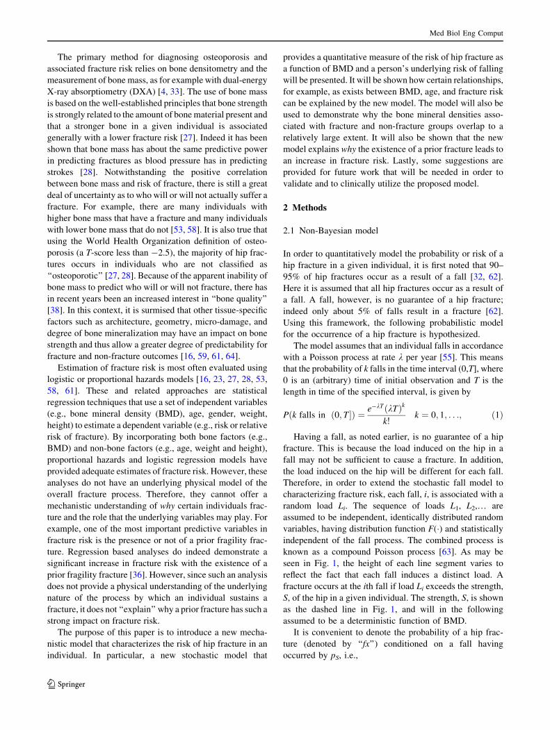
known as a compound Poisson process [63]. As may be

seen in Fig. 1, the height of each line segment varies to

reflect the fact that each fall induces a distinct load. A

fracture occurs at the ith fall if load Li exceeds the strength,

S, of the hip in a given individual. The strength, S, is shown

as the dashed line in Fig. 1, and will in the following

assumed to be a deterministic function of BMD.

It is convenient to denote the probability of a hip frac-

ture (denoted by ‘‘fx’’) conditioned on a fall having

occurred by pS, i.e.,

Med Biol Eng Comput

123

pS ¼ PrðfxjFallÞ ¼ PrðL [ SÞ ð2Þ

In (2), L denotes a generic element of the sequence

{Li, i = 1, 2, …}. Thus, the compound Poisson process as

defined here is a Poisson process which has associated with

each event a probability of a fracture, pS. It is then possible to

extract from this compound Poisson process a thinned

(Poisson) process [15]. In this case, the thinned process is

defined by retaining only the falls that result in a fracture in a

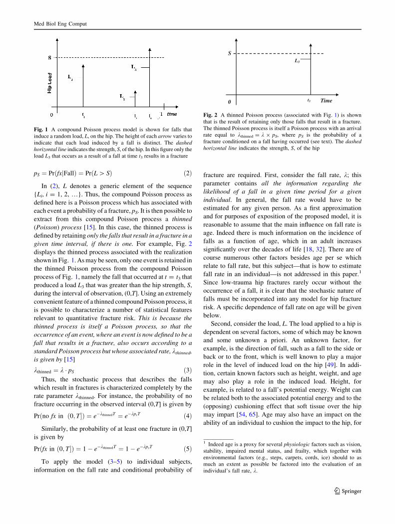
given time interval, if there is one. For example, Fig. 2

displays the thinned process associated with the realization

shown in Fig. 1. As may be seen, only one event is retained in

the thinned Poisson process from the compound Poisson

process of Fig. 1, namely the fall that occurred at t = t3 that

produced a load L3 that was greater than the hip strength, S,

during the interval of observation, (0,T]. Using an extremely

convenient feature of a thinned compound Poisson process, it

is possible to characterize a number of statistical features

relevant to quantitative fracture risk. This is because the

thinned process is itself a Poisson process, so that the

occurrence of an event, where an event is now defined to be a

fall that results in a fracture, also occurs according to a

standard Poisson process but whose associated rate, kthinned,

is given by [15]

kthinned ¼ k � pS ð3ÞThus, the stochastic process that describes the falls

which result in fractures is characterized completely by the

rate parameter kthinned. For instance, the probability of no

fracture occurring in the observed interval (0,T] is given by

Prðno fx in ð0; T �Þ ¼ e�kthinnedT ¼ e�kpsT ð4Þ

Similarly, the probability of at least one fracture in (0,T]

is given by

Prðfx in ð0; T�Þ ¼ 1� e�kthinnedT ¼ 1� e�kpsT ð5Þ

To apply the model (3–5) to individual subjects,

information on the fall rate and conditional probability of

fracture are required. First, consider the fall rate, k; this

parameter contains all the information regarding the

likelihood of a fall in a given time period for a given

individual. In general, the fall rate would have to be

estimated for any given person. As a first approximation

and for purposes of exposition of the proposed model, it is

reasonable to assume that the main influence on fall rate is

age. Indeed there is much information on the incidence of

falls as a function of age, which in an adult increases

significantly over the decades of life [18, 32]. There are of

course numerous other factors besides age per se which

relate to fall rate, but this subject—that is how to estimate

fall rate in an individual—is not addressed in this paper.1

Since low-trauma hip fractures rarely occur without the

occurrence of a fall, it is clear that the stochastic nature of

falls must be incorporated into any model for hip fracture

risk. A specific dependence of fall rate on age will be given

below.

Second, consider the load, L. The load applied to a hip is

dependent on several factors, some of which may be known

and some unknown a priori. An unknown factor, for

example, is the direction of fall, such as a fall to the side or

back or to the front, which is well known to play a major

role in the level of induced load on the hip [49]. In addi-

tion, certain known factors such as height, weight, and age

may also play a role in the induced load. Height, for

example, is related to a fall’s potential energy. Weight can

be related both to the associated potential energy and to the

(opposing) cushioning effect that soft tissue over the hip

may impart [54, 65]. Age may also have an impact on the

ability of an individual to cushion the impact to the hip, for

Fig. 1 A compound Poisson process model is shown for falls that

induce a random load, L, on the hip. The height of each arrow varies to

indicate that each load induced by a fall is distinct. The dashedhorizontal line indicates the strength, S, of the hip. In this figure only the

load L3 that occurs as a result of a fall at time t3 results in a fracture

Time0

S

t3

L3

Fig. 2 A thinned Poisson process (associated with Fig. 1) is shown

that is the result of retaining only those falls that result in a fracture.

The thinned Poisson process is itself a Poisson process with an arrival

rate equal to kthinned = k 9 pS, where pS is the probability of a

fracture conditioned on a fall having occurred (see text). The dashedhorizontal line indicates the strength, S, of the hip

1 Indeed age is a proxy for several physiologic factors such as vision,

stability, impaired mental status, and frailty, which together with

environmental factors (e.g., steps, carpets, cords, ice) should to as

much an extent as possible be factored into the evaluation of an

individual’s fall rate, k.

Med Biol Eng Comput

123

example by reacting with an outstretched hand or by

another neuromuscular reaction (e.g., muscle tightening),

perhaps local to the hip or more generally [18].

Although the load that occurs as a result of a fall is

clearly random, there is presently relatively little empirical

evidence about the specific form of the associated proba-

bility distribution function. There is also relatively little

information on how height, weight, age, and mental status,

among other factors, may be explicitly incorporated into

the conditional probability function (2). In order to deal

with this lack of knowledge, the conditional probability, pS,

is characterized here by a parameterized distribution

function, namely the Weibull distribution given by [48]

FðyÞ ¼ 1� e�ybð Þ

a

; y� 0 ð6Þ

As may be seen, the Weibull distribution is specified by

two parameters, a scale parameter, b, and a power

parameter, a, and as such provides sufficient degrees of

freedom to model a wide range of observed statistical data

[37].

As mentioned above, the underlying model stipulates

that loads {L1, L2, …} are independent random variables

identically distributed according to (6). Therefore, it fol-

lows immediately from (2) and (6) that pS is given by

pS ¼ e�Sbð Þ

a

ð7Þ

A plot of pS as a function of strength, S, for several

choices of the parameter a with b = 1 is shown in Fig. 3.

Note that b is a scale parameter and serves to ‘‘select’’ a

particular portion of the displayed curve, which is plotted

over a wide range of (dimensionless) strength values, S. As

a probability, it ranges from a minimum of zero (achieved

when strength equals infinity and a fall will never result in

a hip fracture) to one (achieved when strength equals zero

and a fall will always result in a hip fracture).

As a further step towards modeling an individual’s risk

of fracture, it is useful to model the strength, S, of the hip as

a function of its BMD, which is denoted by q. Numerous

experimental studies have demonstrated that the strength of

bone can be related to its BMD by a power law function [3,

7, 10, 40, 51]:

S ¼ kqc ð8Þ

In (8), k and c are constants dependent on the specific

experimental conditions (for example, specific geometry

and architecture of the specimen being tested [35, 64]).

Although for regularly shaped specimens of bone (e.g.,

trabecular bone cubes) the exponent c has been shown to

lie between two and three, for intact proximal femurs that

are tested to failure the exponent is smaller (between one

and two) [3, 7, 40]. This may be a result of the different

‘‘densities’’ employed. In the testing of trabecular bone

samples, for example, the density used is usually

proportional to the true volumetric density. However, in

many of the studies involving the evaluation of the strength

of intact femurs, the density is most often the bone mineral

content or areal BMD, both of which can be obtained using

DXA. Another reason for distinct parameter values may be

related to the testing of regularly shaped specimens versus

the testing of whole (intact) bones. In any case the model of

(8) does provide a reasonable estimate of strength by the

proper selection of the associated parameters. Substituting

(8) into (7) allows pS to be expressed as a function of q

pS ¼ e�qbð Þ

a

ð9Þ

Note that in (9) the values for the constants in a and bare distinct from the values of the constants in (7), but for

simplicity we have used the same symbols since the form

of the expression is the same.

Using the above expressions, the probability of at least

one fracture occurring in the time interval (0,T] can then be

expressed as a function of the person-specific fall rate and

BMD, q:2

Fig. 3 The probability of fracture conditioned on a fall having

occurred as a function of strength, S, and for various values of the

parameter, a, using the Weibull probability density function, with

b = 1 (Eq. 7). As may be seen, the conditional probability is a

monotonically decreasing function as strength increases

2 The remainder of this paper will refer only to the occurrence of no

fracture or at least one fracture in a time interval (0,T], because of the

relative simple forms of the expressions in (4) and (5). However,

because of the relative rarity of a fracture event, the probability of at

least one fracture will generally be close to the probability of exactly

one fracture, in a given time interval. In any event, the exact

expressions can easily be substituted if preferred.

Med Biol Eng Comput

123

Prðfx in ð0; T �Þ ¼ 1� e�kTe� q

bð Þa

ð10aÞ

Similarly, the probability of no fracture occurring in

(0,T] can be expressed as

Prðno fx in ð0; T �Þ ¼ e�kTe� q

bð Þa

ð10bÞ

Equation 10a can be used to generate a set of fracture

probabilities for a variety of fall rates and bone mineral

densities. To do this, the fall rate is assumed to be an affine

function of age, k = kage, according to:

kage ¼ a � ageþ b ð11Þ

A number of studies have reported on age-dependent

falls in a variety of populations; from this data we

estimated values of a and b for an age range limited to

40–90 years [20, 31, 32]. In this study, a = 0.02 and

b = -0.7. This produced for example, a fall rate of

k40 = 0.1/year (or 1 fall in a period of 10 years on average)

and a fall rate of k90 = 1.1/year (or 1 fall in a period of

about 0.9 year on average). For this computation, the BMD

ranged between 0.2 and 0.7 g/cm2, in accord with the

variations observed in a population of women measured at

the hip with DXA [47].

The relative risk (RR) of fracture between two groups of

individuals having distinct fall rates (k1 and k2, respec-

tively) and BMD’s (q1 and q2, respectively) over an

interval of observation, T, can also be determined, namely

as follows:

RR ¼ 1� e�k1Te� q1

bð Þa

1� e�k2Te� q2

bð Þa ð12Þ

2.2 Bayesian model

The model presented in the previous section assumed that

the underlying parameters, i.e., the fall rate, k, and the

BMD, q, were fixed and non-random. This means that for a

given individual with fall rate and BMD known a priori, all

the probabilities and statistics relevant to hip fracture can

be computed. Alternatively, it is also possible to take a

different and somewhat more practical perspective. In this

approach, the fall rate and BMD associated with a given

ensemble of individuals are assumed to be random vari-

ables. Generally, the distribution of these random variables,

or some aspect of the distribution such as the means and

variances may be parameterized by an appropriate set of

variables, which are measurable or otherwise known a pri-

ori (such as age). This viewpoint is consistent with the

clinical environment in which a patient is seen by a phy-

sician and for whom no knowledge of fall rate and/or BMD

may be available. Thus, a patient may be considered to

exist within an ensemble of subjects, and onto which a

probabilistic framework is placed.

The extension to such a probabilistic framework for the

fall rate and BMD allows the model to address two key

observations in clinical osteoporosis research for which no

analytic understanding is presently available. Extension of

the model to include random parameters will be explained

in the context of addressing these two key observations.

The first observation is the oft-stated fact that ‘‘there are

many individuals who have low bone mass but do not

fracture while there are many individuals who have higher

mass but do.’’ (See for example [6, 42, 43, 47, 67] for just a

small sampling of the recent literature.) This observation is

often used as an underlying hypothesis for research seeking

other bone but non-mass factors (such as architecture and

geometry for example) that can explain this ‘‘somewhat

confounding’’ observation. However the thinned Poisson

process model can be extended to analyze and explain this

first observation without introducing additional ‘‘bone

quality’’ factors as follows. To do this, assume that the

BMD, q, of each individual in a group of individuals is

distributed as a Normal random variable with mean, l, and

variance, r2, i.e., q *N(l, r2) : g(q). This may for

example, be based on the set of NHANES data that char-

acterizes the mean and variance of BMD as a function of

age, gender, and ethnicity [12, 41]. Assume further that

each individual in the group has a fixed (non-random)

value of fall rate, k0. Then it is possible using Bayes’ rule

to compute the conditional probability density function,

f(q|no fracture in (0,T]), that is the conditional probability

density of BMD conditioned on not having a fracture in the

time interval (0,T], as follows [66]:

f ðqjfx 62 ð0; T �Þ / e�k0Te�ðq=bÞa

� gðqÞ ð13Þ

Using a similar analysis, an expression for the

conditional probability density function, f(q|fx in (0,T]),

that is the conditional probability density of BMD

conditioned on having a fracture in the time interval

(0,T], can be shown to be given by

f ðqjfx 2 ð0; T �Þ / 1� e�k0Te�ðq=bÞa� �� gðqÞ: ð14Þ

Results using these expressions (13), (14) are provided

in the next section.

The second key observation to be analyzed in the con-

text of the present model is that a prior osteoporotic frac-

ture is one of the most significant risk factors that an

individual will suffer another one [11, 26, 29, 36]. The

Poisson process model can help to illuminate why this is so.

The probability that an individual has a fracture in the

interval (T,2T] given a fracture in the interval (0,T] can be

expressed, again using Bayes’ formula, as

Med Biol Eng Comput

123

Pr fx 2 ðT ; 2T� fx 2 ð0j ; T �ð Þ ¼ Prðfx 2 ðT ; 2T�; fx 2 ð0; T �ÞPrðfx 2 ð0; T �Þ :

ð15Þ

In this analysis, the BMD is assumed known (e.g.,

measured), and the fall rate, k, is assumed to be a random

variable. (This is a common clinical situation in which a

patient has received a DXA scan but there is a relatively

large uncertainty in the underlying fall rate.) To simplify

the analysis, the probability distribution, fk(x), for the fall

rate is assumed to be uniform, i.e.,

fkðxÞ ¼1

k2 � k1

�; k1� x� k2; 0; otherwise: ð16Þ

In (16), k1 and k2 are the lower and upper limits,

respectively, of the uniform distribution. This would be

equivalent to having a complete lack of knowledge of a

person’s likelihood of falling short of bounding it from

below and above. The right side of (15) can then be

computed by averaging over the fall rate

Pr fx 2 ðT ; 2T� fx 2 ð0j ; T �ð Þ ¼

Rk2

k1

1� e�kTe�ðq=bÞa

� �2

dk

Rk2

k1

1� e�kTe�ðq=bÞa� �

dk

ð17Þ

A similar analysis can be carried out for obtaining the

probability that an individual has a fracture in the interval

(T,2T] given no fracture in (0,T]. This conditional

probability, expressed as

Pr fx 2 ðT ; 2T� fx 62 ð0j ; T�ð Þ ¼ Prðfx 2 ðT ; 2T�; fx 62 ð0; T�ÞPrðfx 62 ð0; T �Þ

ð18Þ

can then be computed with an expression analogous to (17):

Pr fx 2 ðT; 2T � fx 62 ð0j ; T�ð Þ

¼

Rk2

k1

1� e�kTe�ðq=bÞa

� �� e�kTe�ðq=bÞ

a

dk

Rk2

k1

e�kTe�ðq=bÞa� �

dk

ð19Þ

Equations 17 and 19 can be solved analytically, and the

results are also provided in the next section. As will be

demonstrated, the existence of a prior fracture biases the

value of the conditional probability in (17) towards higher

values; it does this through an implicit expectation that the

fall rate is higher compared with a group of individuals with

the same underlying a priori distribution but who did not

have a prior fracture, biasing the conditional distribution of

(19) towards lower values.

It is also possible to extend this analysis to individuals

whose fall rate and BMD are both unknown and charac-

terized with associated probability distributions (based on

age, for example). In this case, it is expected that there

would be an even greater increase in fracture risk in the

prior fracture group as compared with the group with no

prior fracture. This is because the conditional distribution

of a fracture based on a history of prior fracture will bias

both the fall rate and BMD towards values which increase

fracture risk (i.e., higher fall rate and lower BMD) while no

history of fracture will bias both fall rate and BMD towards

values which decrease fracture risk.

It is worthwhile to examine one additional aspect of the

model in the context of hypothesis testing. The sensitivity

and specificity of a hypothesis testing scheme in order to

classify a subject as a fracture (hypothesis 1 or ‘‘H1’’) case or

a non-fracture (hypothesis 0 or ‘‘H0’’) case is well known in

osteoporosis research [2, 4]. In general, the performance of a

hypothesis test can be assessed through a receiver operating

characteristic (ROC) curve, and in particular through the

area under the ROC curve (AUC) [66]. In osteoporosis,

typical values for AUC in clinical studies are in the range of

0.7–0.8. The search for additional bone quality factors is

directed at least in part towards improving the efficiency of

diagnosing osteoporosis (i.e., increasing AUC values), so

that individuals who will experience a low-trauma fracture

can be correctly identified (‘‘sensitivity’’), while those who

will not suffer a fracture not be identified as a future fracture

case (‘‘specificity’’). In the context of the present model,

consider two cases. In the first, assume that the fall rate and

BMD are both random variables, and that both are observed.

In the second, assume again that fall rate and BMD are both

random variables, but that only BMD is observed. The two

respective ROC curves can be evaluated as follows, in the

context again of a Bayesian analysis.

It can be readily shown using Bayes’ law that the joint

probabilities, f1(q,k|H1), f0(q,k|H0), of BMD (q) and fall

rate (k) under H1 and H0, respectively, are given by

f1ðq; kjH1Þ ¼1� e�kTe

� qbð Þ

a� �gðqÞhðkÞ

PrðH1Þð20Þ

f0ðq; kjH0Þ ¼e�kTe

� qbð Þ

a

gðqÞhðkÞPrðH0Þ

ð21Þ

In (20) and (21), g(q) and h(k) are the a priori

probability density functions of q and k, respectively,

where they are also assumed to be independent of one

another, and Pr(H1) and Pr(H0) are the a priori probabilities

of H1 and H0, respectively.

For the case where both q and k are observed, a likeli-

hood ratio, K2, is formed by dividing (20) by (21), taking

Med Biol Eng Comput

123

the natural logarithm and retaining only those terms

dependent on the measurements, q and k [66]:

K2 ¼ k e�qbð Þ

a

ð22Þ

A ROC curve can be formed by evaluating the

probabilities of K2 conditioned on H1 and H0,

respectively, to be greater than a threshold parameter, g,

which varies over a suitably large range of positive values.

An entirely analogous procedure can be used to deter-

mine the ROC curve for the single measurement (q only)

case. To do this, the probabilities of q conditioned on H1

and H0 are determined by integrating (20) and (21),

respectively, with respect to the fall rate, k. Again, a

likelihood ratio, K1 is formed and the probabilities of K1

conditioned on H1 and H0, respectively, to be greater than a

threshold parameter, g, which varies over a suitably large

range of positive values, are computed. This analysis was

carried out to determine the two ROC curves, using the

following set of parameters. The a priori probability den-

sity for the BMD was assumed normal with a mean of

0.75 g/cm2 and a standard deviation of 0.2 g/cm2. The

a priori probability density for the fall rate k was assumed

to be uniform as in (16), with k1 = 0.05/year and k2 = 5/

year. The other parameters were: a = 1.55, b = 0.4 g/cm2,

and T = 3 years.

3 Results

3.1 Non-Bayesian model

Figure 4 displays the probability of fracture over a time

period of 1 year at each decade of age, as a function of

BMD, which was evaluated using (10a) and (11). Figure 5

displays the RR (12) for individuals having identical fall

rates (k = 0.5/year) but with q1 varying between q2/2 and

2 9 q2, and q2 = 0.25 g/cm2, with a = 1, b = 0.1 g/cm2

and T = 1 year.

3.2 Bayesian model

The two conditional probability functions, (13) and (14),

using k0 = 0.5/year, b = 0.1 g/cm2, a = 1.5, l = 0.4 g/cm2,

r = 0.22 g/cm2, and T = 1 year are plotted in Fig. 6.

As may be seen, there is considerable overlap in the two

conditional probability densities, which arises as a natural

outcome of the stochastic nature of the underlying process

by which hip fractures occur. No additional bone quality

factors were used to derive this result; indeed there is no

Fig. 4 The probability of fracture as a function of BMD, for

individuals of ages 40, 50, 60, 70, 80, and 90 (Eqs. 10a). The fall rate

is assumed to be an affine function of age (Eq. 11)

0.1 0.2 0.3 0.4 0.50

0.5

1

1.5

2

2.5

3

3.5

BMD [g/cm2]

Rel

ativ

e R

isk

Fig. 5 The RR of hip fracture (Eq. 12) for individuals of varying

BMD compared to a reference individual with the same fall rate

(k = 0.5/year) but with a BMD of 0.25 g/cm2. The dashed linesindicate that the RR is one at this density value (0.25 g/cm2)

Fig. 6 The conditional probability density functions of BMD for

subjects who have and have not had a fracture in a time period (0,T],

respectively (Eqs. 13 and 14). As may be seen there is considerable

overlap between the two distributions, analogous to clinical obser-

vations. This overlap is often used as a basis to search for other bone

parameters that can improve estimates of bone strength (over and

above using BMD alone). In this study, bone strength is assumed

known and the overlap arises from the inherent stochastic nature of

the hip fracture process, which includes the randomness of fall

occurrences and the randomness of induced loads at the hip

Med Biol Eng Comput

123

uncertainty in knowledge of bone strength as may be seen

from (8). Note that the fall rate (which was assumed to be

identical in the two conditional distributions) could also be

a random variable with a given distribution; in this case,

the overlap of the two conditional distributions (which can

also be computed using Bayes’ rule) would be expected to

increase even further.

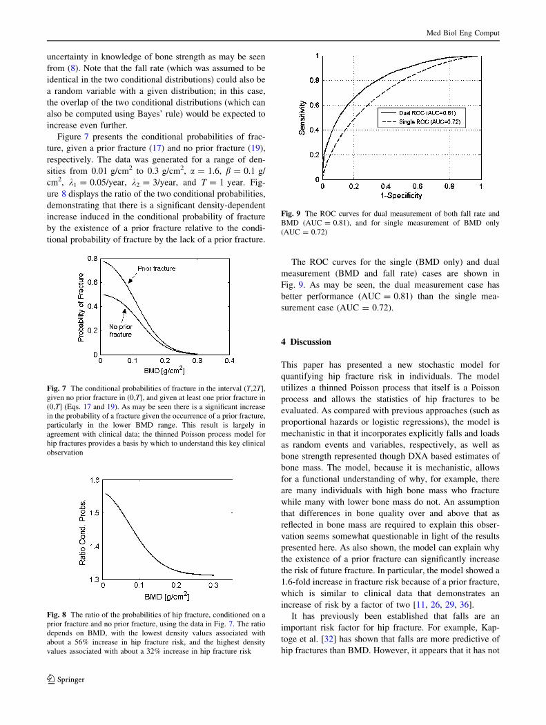
Figure 7 presents the conditional probabilities of frac-

ture, given a prior fracture (17) and no prior fracture (19),

respectively. The data was generated for a range of den-

sities from 0.01 g/cm2 to 0.3 g/cm2, a = 1.6, b = 0.1 g/

cm2, k1 = 0.05/year, k2 = 3/year, and T = 1 year. Fig-

ure 8 displays the ratio of the two conditional probabilities,

demonstrating that there is a significant density-dependent

increase induced in the conditional probability of fracture

by the existence of a prior fracture relative to the condi-

tional probability of fracture by the lack of a prior fracture.

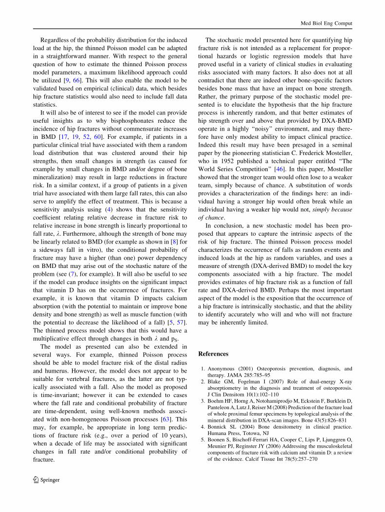
The ROC curves for the single (BMD only) and dual

measurement (BMD and fall rate) cases are shown in

Fig. 9. As may be seen, the dual measurement case has

better performance (AUC = 0.81) than the single mea-

surement case (AUC = 0.72).

4 Discussion

This paper has presented a new stochastic model for

quantifying hip fracture risk in individuals. The model

utilizes a thinned Poisson process that itself is a Poisson

process and allows the statistics of hip fractures to be

evaluated. As compared with previous approaches (such as

proportional hazards or logistic regressions), the model is

mechanistic in that it incorporates explicitly falls and loads

as random events and variables, respectively, as well as

bone strength represented though DXA based estimates of

bone mass. The model, because it is mechanistic, allows

for a functional understanding of why, for example, there

are many individuals with high bone mass who fracture

while many with lower bone mass do not. An assumption

that differences in bone quality over and above that as

reflected in bone mass are required to explain this obser-

vation seems somewhat questionable in light of the results

presented here. As also shown, the model can explain why

the existence of a prior fracture can significantly increase

the risk of future fracture. In particular, the model showed a

1.6-fold increase in fracture risk because of a prior fracture,

which is similar to clinical data that demonstrates an

increase of risk by a factor of two [11, 26, 29, 36].

It has previously been established that falls are an

important risk factor for hip fracture. For example, Kap-

toge et al. [32] has shown that falls are more predictive of

hip fractures than BMD. However, it appears that it has not

Fig. 7 The conditional probabilities of fracture in the interval (T,2T],

given no prior fracture in (0,T], and given at least one prior fracture in

(0,T] (Eqs. 17 and 19). As may be seen there is a significant increase

in the probability of a fracture given the occurrence of a prior fracture,

particularly in the lower BMD range. This result is largely in

agreement with clinical data; the thinned Poisson process model for

hip fractures provides a basis by which to understand this key clinical

observation

Fig. 8 The ratio of the probabilities of hip fracture, conditioned on a

prior fracture and no prior fracture, using the data in Fig. 7. The ratio

depends on BMD, with the lowest density values associated with

about a 56% increase in hip fracture risk, and the highest density

values associated with about a 32% increase in hip fracture risk

Fig. 9 The ROC curves for dual measurement of both fall rate and

BMD (AUC = 0.81), and for single measurement of BMD only

(AUC = 0.72)

Med Biol Eng Comput

123

yet been fully recognized how falls and BMD are quanti-

tatively interconnected in terms of hip fracture prediction.

In a related context, the World Health Organization’s

fracture risk estimation tool (‘‘FRAX’’) does not incorpo-

rate an individual’s likelihood of falling into the compu-

tation of hip fracture risk, stating as justification that

consistent fall data was not available and that pharma-

ceutical intervention has not been shown to reduce fracture

risk in patients selected on the basis of a fall history [30].

However, it has been shown that patients selected on the

basis of risk factors for falling may respond less completely

to agents that preserve bone mass than patients selected on

the basis of low BMD [30]. In view of the present model,

this finding may be explained by the fact that fall rates are

not affected by bone drugs, and thus such patients may not

show as great a response to therapy as expected. In addi-

tion, the expected decrease in hip fracture risk by, for

example, therapeutic increase in BMD (or any factor by

which the strength of a bone increases), as the present

stochastic model demonstrates, is in fact dependent on fall

rate, so that the expected benefit from therapy would also

be fall-rate dependent (see (5)). Indeed, another useful

feature of the proposed model is that it may enable

researchers to determine how much improvement in the

ability to predict hip fracture could be realized if better

estimates of bone strength (i.e., over and above that pro-

vided by DXA-determined BMD) were able to be realized.

For example, hip BMD has been shown to account for up to

88% of the observed variations in femoral strength, as

determined in vitro [13]. The proposed model should be

able to determine if the use of other bone factors (such as

hip axis length, degree of mineralization, cortical thickness

or trabecular architecture) that together with BMD might

explain more of the observed variations in strength, could

in fact significantly impact the estimates of hip fracture

risk. This can be accomplished, for example, by including

varying amounts of noise in the relationship between bone

density and strength, (8), and using computer simulation

techniques [56].

In a related context, the ROC analysis demonstrated that

improvement in performance (as reflected in AUC, for

example) can be achieved when knowledge of fall rate is

included in the measurement space. However, the model

and data presented also demonstrate that there is an upper

bound on such performance. That is to say, even with

perfect knowledge of bone density (strength) and of fall

rate (the likelihood of a fall), there is far from ideal pre-

diction of who will and who will not fracture. That this

may be the fundamental nature of the fracture risk problem

has not been fully appreciated by the osteoporosis research

community.

A seminal study by Hui et al. [24] demonstrated that

fracture risk was age and BMD dependent, with results that

were very similar to the data generated by our model as in

Fig. 4. They also utilized a Poisson model, but did so with

an ad hoc analysis that did not mechanistically seek to

statistically characterize the occurrence of hip fractures.

The model as presented here requires further develop-

ment in order for it to become clinically useful. For

example, methods should be developed in order to estimate

an individual’s fall rate, k. Clearly relying solely on age is

not optimal, and methods which incorporate as many fac-

tors as possible should be studied. Various tests (such as

the ability to rise from a chair without the use of hands)

could also be incorporated into the estimation of fall rate.

Certainly, the prior history of falling would be one key

aspect to include in the estimation procedure. One

approach would be to model the fall rate, k, distributed

a priori as a gamma-distribution. Based on the number of

falls observed a maximum a posteriori estimate of the fall

rate could be made; more falls would lead to a higher

estimate of fall rate. This and other Poisson-mixtures

should be explored in the context of the presently proposed

model.

It will also be necessary to develop additional insights

on the probability distribution function for the load

induced at the hip. The Weibull distribution function was

chosen because of its simplicity and its ability to model a

wide range of statistical phenomena. However, as more

information on load statistics is developed, it may be

helpful to use a different distribution. It may also be

necessary to incorporate additional information into the

load distribution parameters. For example, an age-based

dependence on the parameters may be useful to reflect the

fact that older individuals generally have less ability to

compensate for a fall and will often sustain a higher

induced load at the hip. Similarly, analysis as to how

height and weight affect the induced load and how to

incorporate this information into the distribution param-

eters should also be addressed. For example, as one

extension to the Weibull model, a tri-modal probability

distribution can be utilized, in which one mode models a

fall to the side, another mode models a fall to the front,

while a third mode models a fall to the back. The fall to

the side could use as a mean load the peak force imparted

to the hip in a sideways fall as reported in [54, 65], while

a backwards or forward fall would be associated with

lower mean peak forces, respectively. Additional details

on load statistics could be garnered from other studies,

such as those reporting on the ‘‘biomechanical fracture

threshold’’ [22, 34]. This latter work, although developed

in a deterministic context, could be incorporated into a

more comprehensive specification of the load probability

density function. Additional information on higher order

(e.g., variance) load statistics would need to be deter-

mined by further studies.

Med Biol Eng Comput

123

Regardless of the probability distribution for the induced

load at the hip, the thinned Poisson model can be adapted

in a straightforward manner. With respect to the general

question of how to estimate the thinned Poisson process

model parameters, a maximum likelihood approach could

be utilized [9, 66]. This will also enable the model to be

validated based on empirical (clinical) data, which besides

hip fracture statistics would also need to include fall data

statistics.

It will also be of interest to see if the model can provide

useful insights as to why bisphosphonates reduce the

incidence of hip fractures without commensurate increases

in BMD [17, 19, 52, 60]. For example, if patients in a

particular clinical trial have associated with them a random

load distribution that was clustered around their hip

strengths, then small changes in strength (as caused for

example by small changes in BMD and/or degree of bone

mineralization) may result in large reductions in fracture

risk. In a similar context, if a group of patients in a given

trial have associated with them large fall rates, this can also

serve to amplify the effect of treatment. This is because a

sensitivity analysis using (4) shows that the sensitivity

coefficient relating relative decrease in fracture risk to

relative increase in bone strength is linearly proportional to

fall rate, k. Furthermore, although the strength of bone may

be linearly related to BMD (for example as shown in [8] for

a sideways fall in vitro), the conditional probability of

fracture may have a higher (than one) power dependency

on BMD that may arise out of the stochastic nature of the

problem (see (7), for example). It will also be useful to see

if the model can produce insights on the significant impact

that vitamin D has on the occurrence of fractures. For

example, it is known that vitamin D impacts calcium

absorption (with the potential to maintain or improve bone

density and bone strength) as well as muscle function (with

the potential to decrease the likelihood of a fall) [5, 57].

The thinned process model shows that this would have a

multiplicative effect through changes in both k and pS.

The model as presented can also be extended in

several ways. For example, thinned Poisson process

should be able to model fracture risk of the distal radius

and humerus. However, the model does not appear to be

suitable for vertebral fractures, as the latter are not typ-

ically associated with a fall. Also the model as proposed

is time-invariant; however it can be extended to cases

where the fall rate and conditional probability of fracture

are time-dependent, using well-known methods associ-

ated with non-homogeneous Poisson processes [63]. This

may, for example, be appropriate in long term predic-

tions of fracture risk (e.g., over a period of 10 years),

when a decade of life may be associated with significant

changes in fall rate and/or conditional probability of

fracture.

The stochastic model presented here for quantifying hip

fracture risk is not intended as a replacement for propor-

tional hazards or logistic regression models that have

proved useful in a variety of clinical studies in evaluating

risks associated with many factors. It also does not at all

contradict that there are indeed other bone-specific factors

besides bone mass that have an impact on bone strength.

Rather, the primary purpose of the stochastic model pre-

sented is to elucidate the hypothesis that the hip fracture

process is inherently random, and that better estimates of

hip strength over and above that provided by DXA-BMD

operate in a highly ‘‘noisy’’ environment, and may there-

fore have only modest ability to impact clinical practice.

Indeed this result may have been presaged in a seminal

paper by the pioneering statistician C. Frederick Mosteller,

who in 1952 published a technical paper entitled ‘‘The

World Series Competition’’ [46]. In this paper, Mosteller

showed that the stronger team would often lose to a weaker

team, simply because of chance. A substitution of words

provides a characterization of the findings here: an indi-

vidual having a stronger hip would often break while an

individual having a weaker hip would not, simply because

of chance.

In conclusion, a new stochastic model has been pro-

posed that appears to capture the intrinsic aspects of the

risk of hip fracture. The thinned Poisson process model

characterizes the occurrence of falls as random events and

induced loads at the hip as random variables, and uses a

measure of strength (DXA-derived BMD) to model the key

components associated with a hip fracture. The model

provides estimates of hip fracture risk as a function of fall

rate and DXA-derived BMD. Perhaps the most important

aspect of the model is the exposition that the occurrence of

a hip fracture is intrinsically stochastic, and that the ability

to identify accurately who will and who will not fracture

may be inherently limited.

References

1. Anonymous (2001) Osteoporosis prevention, diagnosis, and

therapy. JAMA 285:785–95

2. Blake GM, Fogelman I (2007) Role of dual-energy X-ray

absorptiometry in the diagnosis and treatment of osteoporosis.

J Clin Densitom 10(1):102–110

3. Boehm HF, Horng A, Notohamiprodjo M, Eckstein F, Burklein D,

Panteleon A, Lutz J, Reiser M (2008) Prediction of the fracture load

of whole proximal femur specimens by topological analysis of the

mineral distribution in DXA-scan images. Bone 43(5):826–831

4. Bonnick SL (2004) Bone densitometry in clinical practice.

Humana Press, Totowa, NJ

5. Boonen S, Bischoff-Ferrari HA, Cooper C, Lips P, Ljunggren O,

Meunier PJ, Reginster JY (2006) Addressing the musculoskeletal

components of fracture risk with calcium and vitamin D: a review

of the evidence. Calcif Tissue Int 78(5):257–270

Med Biol Eng Comput

123

6. Boutroy S, Bouxsein ML, Munoz F, Delmas PD (2005) In vivo

assessment of trabecular bone microarchitecture by high-resolu-

tion peripheral quantitative computed tomography. J Clin Endo-

crinol Metab 90:6508–6515

7. Bouxsein ML, Coan BS, Lee SC (1999) Prediction of the strength

of the elderly proximal femur by bone mineral density and

quantitative ultrasound measurements of the heel and tibia. Bone

25(1):49–54

8. Bouxsein ML, Szule P, Munoz F, Thrall E, Sornay-Rendu E,

Delmas PD (2007) Contribution of trochanteric soft tissues to

force fall estimates, the factor of risk, and prediction of hip

fracture risk. J Bone Miner Res 22(6):825–831

9. Breiman L (1973) Statistics with a view towards applications.

Houghton Mifflin Company, Boston, MA

10. Carter DR, Hayes WC (1977) The compressive behavior of bone

as a two-phase porous structure. J Bone Joint Surg Am 59:954–

962

11. Center JR, Bliue D, Nguyen TV, Eisman JA (2007) Risk of

subsequent fracture after low-trauma fracture in men and women.

JAMA 297(4):387–394

12. Centers for Disease Control and Prevention, U.S. Department Of

Health and Human Services, NHANES - National Health and

Nutrition Examination Survey Web site. Available at: http://www.

cdc.gov/nchs/nhanes.htm. Accessed February 26, 2009

13. Cheng XG, Lowet G, Boonen S, Nicholson PHF, Brys P, Nijs J,

Dequeker J (1997) Assessment of the strength of proximal femur

in vitro: relationship to femoral bone mineral density and femoral

geometry. Bone 20(3):213–218

14. Cooper C, Aihie A (1995) Osteoporosis. Bailliere’s Clin Rheu

9(3):555–564

15. Cox DR, Isham V (1980) Point processes. CRC Press, Boca

Raton, FL

16. Cummings SR, Nevitt MC, Browner WS, Stone K, Fox KM,

Ensrud KE, Cauley J, Black D, Vogt TM (1995) Risk factors for

hip fracture in white women. New Engl J Med 332(12):767–774

17. Cummings SR, Karpf DB, Harris F et al (2002) Improvement in

spine bone density and reduction in risk of vertebral fractures

during treatment with antiresorptive drugs. Am J Med 112:281–

289

18. Dargent-Molina P, Favier F, Grandjean H, Baudoin C, Schott

AM, Hausherr E, Meunier PJ, Breart G, for EPIDOS Group

(1996) Fall-related factors and risk of hip fracture: the EPIDOS

prospective study. Lancet 348:145–149

19. Eastell R, Barton I, Hannon RA, Chines A, Garnero P, Delmas

PD (2003) Relationship of early changes in bone resorption to the

reduction in fracture risk with risendronate. J Bone Miner Res

18:1051–1056

20. Gregg EW, Pereira MA, Caspersen CJ (2000) Physical activity,

falls, and fractures among older adults: a review of the epide-

miologic evidence. J Am Geriatr Soc 48(8):883–893

21. Gullberg B, Johnell O, Kanis JA (1997) World-wide projections

for hip fracture. Osteoporos Int 7:407

22. Hayes WC, Piazza SJ, Zysset PK (1991) Biomechanics of frac-

ture risk prediction of the hip and spine by quantitative computed

tomography. Radiol Clin North Am 29:1–18

23. Hosmer DW Jr, Lemeshow S (1989) Applied logistic regression.

John Wiley, New York

24. Hui SL, Slemenda CW, Johnston CC Jr (1988) Age and bone

mass as predictors of fracture in a prospective study. J Clin Invest

81:1804–1809

25. International Osteoporosis Foundation. 2009 Facts and statistics

about osteoporosis and its impact. International Osteoporosis

Foundation Web site. Available at: http://www.iofbonehealth.org/

facts-and-statistics.html. Accessed February 24, 2009

26. Johnell O, Kanis JA, Oden A, Sernbo I, Redlund-Johnell I,

Petterson C, De Laet C, Jonsson B (2004) Fracture risk following

an osteoporotic fracture. Osteoporos Int 15:175–179

27. Johnell O, Kanis JA, Oden A, Johansson H, De Laet C, Delmas P,

Eisman JA, Fujiwara S, Kroger H, Mellstrom D, Meunier PJ,

Melton LJ III, O’Neill T, Pols H, Reeve J, Silman A, Tenenhouse

A (2005) Predictive value of BMD for hip and other fractures.

J Bone Miner Res 20:1185–1194

28. Kanis JA (2002) Diagnosis of osteoporosis and assessment of

fracture risk. Lancet 359(9321):1929–1936

29. Kanis JA, Johnell O, De Laet C, Johansson H, Oden A, Delmas P

et al (2004) A meta-analysis of previous fracture and subsequent

fracture risk. Bone 35:375–382

30. Kanis JA, Johnell O, Oden A, Johansson H, McCloskey E (2008)

FRAXTM and the assessment of fracture probability in men and

women from the UK. Osteoporos Int 19:385–397

31. Kannus P, Sievanen H, Palvanen M, Jarvinen T, Parkkari J (2005)

Prevention of falls and consequent injuries in elderly people.

Lancet 366:1885–1893

32. Kaptoge S, Benevolenskaya LI, Bhalla AK, Cannata JB, Boonen

S, Flach JA et al (2005) Low BMD is less predictive than

reported falls for future limb fractures in women across Europe:

results from the European Prospective Osteoporosis Study. Bone

36:387–398

33. Kaufman JJ, Siffert RS (2001) Non-invasive assessment of bone

integrity. In: Cowin S (ed) Bone mechanics handbook. CRC

Press, Boca Raton, FL, pp 34.1–34.25

34. Keaveny TM, Bouxsein ML (2008) Theoretical implications of

the biomechanical fracture threshold (Perspective). J Bone Miner

Res 23(10):1541–1547

35. Keaveny TM, Morgan EF, Niebur GL, Yeh OC (2001) Biome-

chanics of trabecular bone. Annu Rev Biomed Eng 3:307–333

36. Klotzbuecher CM, Ross PD, Landsman PB, Abbott TA III,

Berger M (2000) Patients with prior fractures have an increased

risk of future fractures: a summary of the literature and statistical

synthesis. J Bone Miner Res 15(4):721–739

37. Lawless JF (1982) Statistical models and methods for lifetime

data. Wiley, New York, NY

38. Lester G (2005) Bone quality: summary of NIH/ASBMR meet-

ing. J Musculoskelet Neuronal Interact 5:309

39. Lin JT, Lane JM (2004) Osteoporosis: a review. Clin Orthop

Relat Res 425:126–134

40. Lochmuller EM, Miller P, Burklein D, Wehr U, Rambeck W,

Eckstein F (2000) In situ femoral dual-energy X-ray absorpti-

ometry related to ash weight, bone size and density, and its

relationship with mechanical failure loads of the proximal femur.

Osteoporos Int 11:361–367

41. Looker AC, Orwoll ES, Conrad Johnston C Jr, Lindsay RL,

Wahner HW, Dunn WL, Calvo MS, Harris TB, Heyse SB (1997)

Prevalence of low femoral bone density in older U.S. adults from

NHANES III. J Bone Miner Res 12:1761–1768

42. Mc Donnell P, Mc Hugh PE, O’Mahoney D (2007) Vertebral

osteoporosis and trabecular bone quality. Ann Biomed Eng

35(2):170–189

43. McCreadie BR, Goldstein SA (2000) Biomechanics of fracture: is

bone mineral density sufficient to assess risk? J Bone Miner Res

15(12):2305–2308

44. Melton LJ III (1988) Epidemiology of fractures. In: Riggs BL,

Melton LJ III (eds) Osteoporosis: etiology, diagnosis, and man-

agement. Raven Press, New York, NY, pp 133–154

45. Miller CW (1978) Survival and ambulation following hip frac-

ture. J Bone Joint Surg 60A:930–934

46. Mosteller F (1952) The world series competition. J Am Stat

Assoc 47(259):355–380

Med Biol Eng Comput

123

47. Orwoll ES, Marshall LM, Nielson CM, Cummings SR, Lapidus J,

Cauley JA, Ensrud K, Lane N, Hoffman PR, Kopperdahl DL,

Keaveny TM, for the Osteoporotic Fractures in Men Study Group

(2009) Finite element analysis of the proximal femur and hip

fracture risk in older men. J Bone Miner Res 24(3):475–483

48. Papoulis A, Pillai SU (2002) Probability, random variables and

stochastic processes, 4th edn. McGraw Hill, New York, NY

49. Pinilla TP, Boardman KC, Bouxsein ML, Myers ER, Hayes WC

(1996) Impact direction from a fall influences the failure load of

the proximal femur as much as age-related bone loss. Calcif

Tissue Int 58:231–235

50. Reginster J-Y, Burlet N (2006) Osteoporosis: a still increasing

prevalence. Bone 38(2 Supp1):4–9

51. Rice JC, Cowin SC, Bowman JA (1988) On the dependence of

the elasticity and strength of cancellous bone on apparent density.

J Biomech 21(2):155–168

52. Riggs BL, Melton LJ III (2002) Bone turnover matters: the ra-

loxifene treatment paradox of dramatic decreases in vertebral

fractures without commensurate increases in bone density. J Bone

Miner Res 17:11–14

53. Robbins JA, Schott AM, Garnero P, Delmas PD, Hans D, Meu-

nier PJ (2005) Risk factors for hip fracture in women with high

BMD: EPIDOS study. Osteoporos Int 16:149–154

54. Robinovich SN, Hayes WC, McMahon TA (1991) Prediction of

femoral impact forces in falls on the hip. Trans ASME 113:366–

374

55. Ross S (1995) Stochastic processes, 22nd edn. Wiley, New York

56. Ross SM (2006) Simulation, 4th edn. Elsevier Science and

Technology Books, Amsterdam, The Netherlands

57. Roux C, Bischoff-Ferrari HA, Papapoulos SE, de Papp AE, West

JA, Bouillon R (2008) New insights into the role of vitamin D

and calcium in osteoporosis management: an expert roundtable

discussion. Curr Med Res Opin 24(5):1363–1370

58. Schuit SC, van der Klift M, Weel AE, de Laet CE, Burger H, Seeman

E, Hofman A, Uitterlinden AG, van Leeuwen JP, Pols HA (2004)

Fracture incidence and association with bone mineral density in

elderly men and women: the Rotterdam Study. Bone 34:195–202

59. Seeman E (2008) Bone quality: the material and structural basis

of bone strength. J Bone Miner Metab 26(1):1–8

60. Siffert RS, Kaufman JJ (2007) Ultrasonic bone assessment: ‘‘the

time has come’’. Bone 40(1):5–8

61. Siffert RS, Luo GM, Cowin SC, Kaufman JJ (1996) Dynamic

relationships of trabecular bone density, architecture, and strength

in a computational model of osteopenia. Bone 18(2):197–206

62. Silva MJ (2007) Biomechanics of osteoporotic fractures. Injury

38(Suppl 3):S69–S76

63. Snyder DL, Miller MI (1975) Random point processes. Wiley,

New York, NY

64. Turner C (2002) Biomechanics of bone: determinants of skeletal

fragility and bone quality. Osteoporos Int 13(2):97–104

65. van den Kroonenberg A, Hayes W, McMahon TA (1996) Hip

impact velocities and body configurations for experimental falls

from standing height. J Biomech 29:807–811

66. Van Trees HL (1968) Detection, estimation, and modulation

theory part I. Wiley, New York

67. Yang L, Peel N, Clowes JA, McCloskey EV, Eastell R (2009)

Use of DXA-based structural engineering models of the proximal

femur to discriminate hip fracture. J Bone Miner Res 24(1):33–42

Med Biol Eng Comput

123