a piecewise line-search technique for maintaining the positive definitenes of the matrices in the...
TRANSCRIPT
Computational Optimization and Applications, 16, 121–158, 2000c© 2000 Kluwer Academic Publishers. Manufactured in The Netherlands.
A Piecewise Line-Search Technique for Maintainingthe Positive Definiteness of the Matricesin the SQP Method
PAUL ARMAND [email protected] ESA CNRS 6090 - Departement de Mathematiques - 123, av. A. Thomas - 87060 Limoges Cedex, France
J. CHARLES GILBERT [email protected] Rocquencourt, BP 105, 78153 Le Chesnay Cedex, France
Received February 12, 1997; Accepted January 20, 1999
Abstract. A technique for maintaining the positive definiteness of the matrices in the quasi-Newton version of theSQP algorithm is proposed. In our algorithm, matrices approximating the Hessian of the augmented Lagrangianare updated. The positive definiteness of these matrices in the space tangent to the constraint manifold is ensuredby a so-called piecewise line-search technique, while their positive definiteness in a complementary subspace isobtained by setting the augmentation parameter. In our experiment, the combination of these two ideas leads to anew algorithm that turns out to be more robust and often improves the results obtained with other approaches.
Keywords: BFGS formula, equality constrained optimization, piecewise line-search, quasi-Newton algorithm,successive quadratic programming
1. Introduction
We consider from a numerical point of view the nonlinear equality constrained optimizationproblem
minimize f (x)
subject to c(x) = 0, x ∈ Ä, (1.1)
whereÄ is an open set ofRn and the two functionsf :Ä→ Randc :Ä→ Rm (1≤ m< n)are sufficiently smooth. Although constrained optimization problems often present inequal-ity constraints also, studying (1.1) is of interest. Such a study can indeed be consideredas a first stage in the analysis of more general settings. Also, the nonlinear interior pointapproach for dealing with inequalities often transform the original problem in a series ofproblems with equality constraints only by introducing and penalizing slack variables (see[5] and the references therein). The algorithms presented in this paper could be adapted tothis approach. Finally, it happens that problems with equality constraints only are encoun-tered.
122 ARMAND AND GILBERT
Since the setÄ in (1.1) is open, it does not define general constraints. It is just the seton which good properties off andc hold. For example, we will always suppose that thefollowing assumption hold.
General Assumption: for all x ∈ Ä, them×n Jacobian matrix ofc atx, denoted byA(x)= ∇c(x)>, has full rank.
The Lagrangian function associated with problem (1.1) is defined onÄ× Rm by
`(x, λ) = f (x)+ λ>c(x), (1.2)
whereλ ∈ Rm is called theLagrange multiplier. The first order optimality conditions ofproblem (1.1) at a local solutionx∗ with associated multiplierλ∗ can be written
∇ f∗ + A>∗λ∗ = 0 and c∗ = 0. (1.3)
Throughout the paper, we use the notationf∗ = f (x∗), ∇ f∗ = ∇ f (x∗), A∗ = A(x∗), etc.Also, we assume that the second order sufficient conditions of optimality hold at(x∗, λ∗).Using the notationL∗ = ∇2
xx`(x∗, λ∗), this can be written
h>L∗h > 0, for all h 6= 0 such thatA∗h = 0. (1.4)
The sequential quadratic programming (SQP) algorithm is a Newton-like method in(x, λ)applied to the first order optimality conditions (1.3) (see for example Fletcher [14], Bonnanset al. [4], or the survey paper [2]). Thekth iteration of the algorithm can be described asfollows. Given an iterate pair(xk, λk) ∈ Ä × Rm, approximating a solution pair(x∗, λ∗),the followingquadratic subproblemis solved ford ∈ Rn:
min ∇ fk>d + 1
2d>Mkd
s.t. ck + Akd = 0.(1.5)
We adopt the notationfk = f (xk), ∇ fk = ∇ f (xk), ck = c(xk), Ak = A(xk), etc. In (1.5),it is suitable to take forMk the Hessian of the Lagrangian or an approximation to it. Let usdenote by(dk, λ
QP
k ) a primal-dual solution of (1.5), i.e., a solution of its optimality conditions
∇ fk + Mkdk + A>kλQP
k = 0 and ck + Akdk = 0. (1.6)
The link between (1.3) and (1.5) is that, whenMk is the Hessian of the Lagrangian,(dk, λQP
k −λk) is the Newton step for the system (1.3) at(xk, λk).
Close to a solution, it is then desirable that the algorithm updates(xk, λk) by xk+1 =xk+ dk andλk+1 = λQP
k . To ensure convergence from remote starting points, however, thedirectiondk is often used as a search direction, along which a stepsizeαk > 0 is chosen.The stepsize is adjusted such that the next iterate
xk+1 = xk + αkdk,
reduces sufficiently the value of some merit function.
PIECEWISE LINE-SEARCH FOR THE SQP ALGORITHM 123
This paper deals with the quasi-Newton version of the SQP algorithm: the matrixMk isupdated at each iteration by a formula, whose aim is to makeMk closer to some Hessian,typically the Hessian of the Lagrangian or the Hessian of the augmented Lagrangian. Insuch a method, it is convenient to forceMk to be positive definite, so thatdk is a descentdirection of the merit function. This can be achieved by using the BFGS formula: for somevectorsγk andδk in Rn,
Mk+1 = Mk − Mkδkδ>k Mk
δ>k Mkδk+ γkγ
>k
γ>k δk. (1.7)
This formula is interesting because, as this is well known, the positive definiteness of theupdated matrices is sustained fromMk to Mk+1 if and only if the following curvatureconditionholds:
γ>k δk > 0. (1.8)
Therefore, if the initial matrixM0 is positive definite and if (1.8) is realized at each iteration,all the matricesMk will be positive definite. One of the aims of this paper is to propose atechnique to realize this curvature condition in a consistent manner at each iteration. Thisis not an easy task, as we now explain.
WhenMk is taken as an approximation of the Hessian of the Lagrangian, it makes senseto take forγk in (1.7) the vector
γ `k = ∇x`(xk+1, λ)−∇x`(xk, λ), (1.9)
whereλ is some multiplier, usuallyλQP
k , since this change in the gradient of the Lagrangiangives information on the Hessian of the Lagrangian. However, the lack of positive defi-niteness ofL∗ makes this approach difficult. Indeed, with this choice ofγk, the curvaturecondition may never be realized for any displacementδk = xk+1− xk alongdk, because theLagrangian may have negative curvature along this direction, even close to the solution.
The idea of modifying the vectorγ `k to force satisfaction of the curvature condition goesback at least to Powell [30], who has suggested choosingγk as a convex combination ofγ `kandMkδk:
γ Pk = θγ `k + (1− θ)Mkδk. (1.10)
In (1.10),θ is the number in(0, 1], the closest to 1, such that the inequality(γ P
k
)>δk ≥ η δ>k Mkδk
is satisfied. The constantη is set to 0.2 in [30] and to 0.1 in [31]. Powell’s correction ofγ `kis certainly the most widely used technique in practice. Its success is due to its appealingsimplicity and its usually good numerical performance. The fact that it may encounterdifficulties partly motivates the present study (see [31] or [32, p. 125]). Another motivationis that the best known result obtained so far on the speed of convergence with Powell’s
124 ARMAND AND GILBERT
correction (precisely, ther -superlinear convergence, see [29]) is not as good as one canreasonably expect, which is theq-superlinear convergence.
Another modification ofγ `k consists in taking forγk an approximation of the changein the gradient of the augmented Lagrangian, which is the function (1.2) to which theaugmentation termr
2‖c(x)‖2 is added (‖·‖ denotes the2-norm). This idea, proposed byTapia [36], has roots in the work of Han [22] and Tapia [35] and was refined later by Byrd,Tapia, and Zhang [8] (BTZ for short). In the augmented Lagrangian-based method of BTZ,the vectorγk is set to
γ Sk = γ `k + rk A>k+1Ak+1δk, (1.11)
where the augmentation parameterrk is the smallest nonnegative number such that(γ S
k
)>δk ≥ max
{∣∣(γ `k )>δk
∣∣, νBTZ‖Ak+1δk‖2}. (1.12)
In the implementation of the algorithm given in [8], the authors setνBTZ = 0.01. It is clearthat this approach does not work whenAk+1δk = 0 and(γ `k )
>δk < 0. In this case, theauthors propose the following “back-up strategy”: when (1.12) does not hold withrk = 0and
‖Ak+1δk‖ < min{βBTZ, ‖δk‖}‖δk‖, (1.13)
whereβBTZ is a small positive number (the value 0.01 is chosen in [8]), then the vectorA>k+1Ak+1δk in (1.11) is replaced byδk andrk is set such that (1.12) is satisfied. In [8],assuming the convergence of(xk, λk) to (x∗, λ∗), a unit stepsize, and a matrix updatedby the BFGS formula, it is shown that the sequence{xk} convergesr -superlinearly tox∗.Furthermore, numerical experiments demonstrate that the technique is competitive withPowell’s correction. The back-up strategy used in the BTZ algorithm is, however, not veryattractive. Indeed, when it is active, the pair(γ S
k , δk) refers to a matrix different from theHessian of the Lagrangian or the Hessian of the augmented Lagrangian, modifying thesearch directiondk in a way that is not supported by the theory.
The present paper develops a new approach, which uses a stepsize determination processto realize the curvature condition (1.8). Therefore, the new method can be viewed as anextension of a well established technique in unconstrained optimization, which uses theWolfe line-search to obtain (1.8) (see [12, 24, 37, 38]).
Our algorithm combines two ideas. On the one hand, the Wolfe line-search technique usedin unconstrained optimization and the experience acquired with reduced Hessian methodsfor equality constrained problems [18, 20] have shown that an appropriate move along theconstraint manifold{x : c(x)= ck} can take care of the positive definiteness of the “tangentpart” of the matricesMk. The tangent or longitudinal component of the displacement(i.e., along the constraint manifold) is determined by a specific algorithm, that we callpiecewise line-search(PLS for short). Its aim is to realized a so-calledreduced Wolfecondition, which will be introduced in Section 3 (see formula (3.4)). By this, we mimicwhat is done in unconstrained optimization, where the curvature condition is fulfilled bya line-search algorithm satisfying the Wolfe conditions (see for instance [24, Chap. II,
PIECEWISE LINE-SEARCH FOR THE SQP ALGORITHM 125
§ 3.3]). In constrained optimization, this approach is more delicate, however, since thecurvature condition (1.8) withγk = γ `k may never hold along a straight line (recall thatthe Lagrangian may have negative curvature along the SQP direction). Nevertheless, wewill show that there is a path defined by a particular differential equation along whichthe reduced Wolfe condition can be realized. The PLS technique consists in followinga piecewise linear approximation of this “guiding path”, each discretization point beingsuccessively chosen by means of an Armijo line-search process along intermediate searchdirections. An important aspect of this approach is that it is readily adapted to a globalframework, being able to force convergence from remote starting points.
On the other hand, for the “transversal part” of the matricesMk, we follow the BTZapproach and incorporate in the vectorγk a term of the formrk A>k Akδk:
γk = γk + rk A>k Akδk, whereγk ' L∗δk.
The explicit form ofγk will be stated in Section 3.1. The specificity of our algorithm is that,because of the realization of the reduced Wolfe condition and the structure of the vectorγk,the curvature condition (1.8) can always be satisfied, even whenAkδk = 0. This is quitedifferent from the BTZ approach, for which a back-up strategy is necessary.
This is the third paper describing how the PLS technique can be used to maintain thepositive definiteness of the updated matrices in quasi-Newton algorithms for solving equalityconstrained problems. The approach was first introduced in [18] in the framework of reducedquasi-Newton algorithms, in which the updated matrices approach the reduced Hessianof the Lagrangian. In that paper, the vectorγk is a difference of reduced gradients, bothevaluated asymptotically in the same tangent space. In a way, this is the reference algorithm,since it may be viewed as a straightforward generalization of the Wolfe line-search toequality constrained problems. It has however the inconvenience to require at least twolinearizations of the constraints per iteration. For some problems, this may be an excessiveextra cost. For this reason, an approach that requires asymptotically only one linearizationof the constraints per iteration is developed in [20]. In that paper also, the technique isintroduced for reduced quasi-Newton algorithms. The present paper shows how the PLStechnique can be used within the SQP (or full Hessian) algorithm.
To conclude this introduction, let us mention that there are other ways of implementingquasi-Newton algorithms for equality constraint minimization. Coleman and Fenyes [11],Biegler, Nocedal, and Schmid [1], and Gurwitz [21] update separately approximations ofdifferent parts of the Hessian of the Lagrangian. Another possibility is to use quasi-Newtonversions of the reduced Hessian algorithm, in which approximations of the reduced Hessianof the Lagrangian are updated. This is attractive since this matrix is positive definite neara regular solution. Also, by contrast to the full Hessian method presented in this paper,which is appropriate for small or medium scale problems, this approach can also be used forlarge scale problems so long as the ordern−m of the reduced Hessian remains small. Thereduced Hessian approach has, however, its own drawbacks: either the constraints have tobe linearized twice per iteration, which is sometimes an important extra cost, or an updatecriterion has to be introduced, which does not always give good numerical results. We referthe reader to [7, 10, 17, 18, 20, 27, 39] for further developments along that line.
126 ARMAND AND GILBERT
The paper is organized as follows. In Section 2, we make precise our notation, the formof the SQP direction, and our choice of merit function. Section 3 presents our approachto satisfying the curvature condition (1.8) and outlines the PLS technique. Section 4 showsthe finite termination of the search algorithm. In comparison with the material presentedin [18], this result is proved in a more straightforward manner and it is less demandingon the way the intermediate stepsizes are determined. The overall minimization algorithmis given in Section 5. As we have mentioned, this algorithm is immediately expressed ina global setting. Therefore, in this section, we can concentrate on its global convergencerather than on its local properties. We also give conditions assuring the admissibility of theunit stepsize, which will lead to a criterion selecting the iterations at which the PLS has tobe launched. Section 6 gives more details on implementation issues and Section 7 relatesthe results of numerical tests. The paper terminates with a conclusion section.
2. Background material and notation
Let us first introduce two decompositions ofRn that will be useful throughout the paper.Each of them decomposes the variable space into two complementary subspaces and ischaracterized by a triple(Z−(x), A−(x), Z(x)). The columns of the matricesZ−(x) andA−(x) span the two complementary subspaces andZ(x) is deduced fromZ−(x), A−(x),andA(x).
In the first decomposition,Z−(x) and A−(x) can be considered as an additional dataon the structure of the problem. These operators andZ(x) have to satisfy the followingproperties.
• Z−(x) is ann×(n−m)matrix, whose columns form a basis of the null spaceN (A(x))of A(x):
A(x)Z−(x) = Om×(n−m). (2.1)
• A−(x) is ann×m right inverse ofA(x):
A(x)A−(x) = Im. (2.2)
In particular, the columns ofA−(x) form a basis of a subspace complementary toN (A(x)).• Z(x) is the unique(n−m)× n matrix such that
Z(x)Z−(x) = In−m and Z(x)A−(x) = 0(n−m)×m. (2.3)
From these properties, we can deduce the following identity:
A−(x)A(x)+ Z−(x)Z(x) = In. (2.4)
Using (2.2) and (2.3), we see thatA−(x)A(x) andZ−(x)Z(x) are slant projectors on therange space ofA−(x) and the complementary subspaceN (A(x)). For a motivation of this
PIECEWISE LINE-SEARCH FOR THE SQP ALGORITHM 127
choice of notation and for practical examples of operatorsA−(x) and Z−(x), see Gabay[15].
From these operators, the notions of reduced gradient and Lagrange multiplier estimatecan be introduced. Thereduced gradientof f at x is defined by
g(x) = Z−(x)>∇ f (x). (2.5)
Using (2.1), we haveg(x) = Z−(x)>∇x`(x, λ∗), so that
∇g>∗ = Z−>∗ L∗. (2.6)
The first equation in (1.3) and (2.2) imply thatλ∗ = −A−>∗ ∇ f∗. Therefore, the vector
λ(x) = −A−(x)>∇ f (x). (2.7)
can be considered as aLagrange multiplier estimate. Similarly, using (2.2), we haveλ(x) =−A−(x)>∇x`(x, λ∗)+ λ∗, so that
∇λ>∗ = −A−>∗ L∗. (2.8)
The second useful decomposition ofRn differs from the first one by the choice of thesubspace complementary toN (A(x)). It comes from the form of the solution of the quadraticsubproblem (1.5) and therefore it depends only on the problem data. LetMk be the currentHessian approximation with the property thatZ−(x)>Mk Z−(x) is positive definite, anddefine
Hk(x) = (Z−(x)>Mk Z−(x))−1.
Let x be a point inÄ and consider the quadratic subproblem ind ∈ Rn:
min ∇ f (x)>d + 12 d>Mkd
s.t. c(x)+ A(x)d = 0.(2.9)
Let us denote by(dQP
k (x), λQP
k (x)) the primal-dual solution of (2.9). Using the first decom-position ofRn at x, it is not difficult to see that the primal solution can be written (see alsoGabay [16])
dQP
k (x) = −Z−(x)Hk(x)g(x)− (I − Z−(x)Hk(x)Z−(x)>Mk)A
−(x)c(x). (2.10)
Using (2.1) and (2.2), we find that the factor ofc(x) in (2.10) satisfies
A(x)[(I − Z−(x)Hk(x)Z−(x)>Mk)A
−(x)] = Im.
Hence, the product of matrices inside the square brackets forms a right inverse ofA(x),which is denoted byA−k (x). Defining
Zk(x) = Hk(x)Z−(x)>Mk, (2.11)
128 ARMAND AND GILBERT
we have
A−k (x) = (I − Z−(x)Zk(x))A−(x), (2.12)
and thus (2.10) can be rewritten
dQP
k (x) = −Z−(x)Hk(x)g(x)− A−k (x)c(x). (2.13)
We have built a triple(Z−(x), A−k (x), Zk(x)) satisfying conditions (2.1), (2.2), and (2.3),hence defining suitably a second decomposition ofRn. In particular, we have
A−k (x)A(x)+ Z−(x)Zk(x) = In. (2.14)
Note that despite the fact thatA−(x) and Z−(x) are used in formula (2.12), the operatorA−k (x)does not depend on the choice of right inverse and tangent basis. Indeed,−A−k (x)c(x)is also defined as the solution of the quadratic subproblem (2.9) in which∇ f (x) is set tozero (see also formula (4.7) in the proof of Lemma 4.3 below).
In order to simplify the notation, we denote byZk and A−k the matricesZk(xk) andA−k (xk). With this convention, the solutiondk of the quadratic subproblem (1.5) can bewritten
dk = −Z−k Hkgk − A−k ck. (2.15)
The vectorZkdk = −Hkgk is called thereduced tangent direction.Using Zk(x)A
−k (x)= 0 and the nonsingularity ofHk(x), we have from (2.11) the follow-
ing useful identity
Z−(x)>Mk A−k (x) = 0(n−m)×m, (2.16)
which means that the tangent spaceN (A(x))and the range space ofA−k (x)are perpendicularfor the scalar product associated withMk. In particular, ifL∗ is used in place ofMk in theprevious equality and ifx = x∗, we obtain
Z−>∗ L∗ A−∗ = 0. (2.17)
With (2.6), this shows that the columns ofA−∗ form a basis of the space tangent to the reducedgradient manifold{g= 0} atx∗. Therefore, from (2.15), we see that the SQP directiondk hasa longitudinal component−Z−k Hkgk, tangent to the manifold{c = ck}, and atransversalcomponent−A−k ck, which tends to be tangent to the manifold{g = gk} when the pair(xk, Z−>k Mk) is close to(x∗, Z−>∗ L∗).
In this paper, the globalization of the SQP method follows the approach of Bonnans [3].We take as merit function the nondifferentiable augmented Lagrangian
2µ,σ (x) = f (x)+ µ>c(x)+ σ‖c(x)‖P , (2.18)
PIECEWISE LINE-SEARCH FOR THE SQP ALGORITHM 129
in whichµ ∈ Rm, σ is a positive number, and‖·‖P is an arbitrary (primal) norm onRm.This norm may differ from the2-norm and it is not squared in2µ,σ . We denote by‖·‖D
the dual norm associated with‖·‖P with respect to the Euclidean scalar product:
‖u‖D = sup‖v‖P=1
u>v.
The penalty function2µ,σ is convenient for globalizing the SQP method for at least tworeasons. On the one hand, the penalization is exact, provided theexactness condition
‖µ− λ∗‖D < σ (2.19)
holds (see for example Han and Mangasarian [23], and Bonnans [3]). On the other hand,the Armijo inequality using this function accepts the unit stepsize asymptotically, undersome natural conditions (this is analyzed in Section 5, see also [3]).
We recall that(ψ ◦φ) has directional derivatives at a pointx, if ψ is Lipschitz continuousin a neighborhood ofφ(x) and has directional derivatives atφ(x), and ifφ has directionalderivatives atx. Furthermore,(ψ ◦ φ)′(x; h) = ψ ′(φ(x);φ′(x; h)). In particular, due toits convexity, a norm has the properties of the functionψ above, and sincef andc aresupposed smooth,2µ,σ has directional derivatives.
We conclude this section by giving formulae for the directional derivatives of2µ,σ andby giving conditions for having descent directions. Letd be a vector ofRn satisfying thelinear constraintsc(x)+ A(x)d = 0. The directional derivative of2µ,σ atx in the directiond is given by
2′µ,σ (x; d) = ∇ f (x)>d − µ>c(x)− σ‖c(x)‖P (2.20)
(for the differentiation of the term with the norm, use the very definition of directionalderivative, see for example [20]). For any multiplierλ, we then have
2′µ,σ (x; d) = ∇x`(x, λ)>d + (λ− µ)>c(x)− σ‖c(x)‖P . (2.21)
Therefore, ifd is a descent direction of the Lagrangian function at(x, λ), in the sense that∇x`(x, λ)>d < 0 (which in particular holds for the directiondk when(x, λ) = (xk, λ
QP
k )),thend is also a descent direction of2µ,σ at x provided thedescent condition
‖λ− µ‖D ≤ σ (2.22)
holds (compare with the exactness condition (2.19)).
3. The approach
This section describes our quasi-Newton version of the SQP algorithm in a global frame-work. Our aim is to develop a consistent way of updating the positive definite matrixMk,using adequate vectorsγk andδk.
130 ARMAND AND GILBERT
3.1. Computation ofγk
As we said in the introduction, we forceMk to be an approximation of the Hessian of theaugmented Lagrangian. This is equivalent to considering the problem
min f (x)+ r
2‖c(x)‖2
s.t. c(x) = 0, x ∈ Ä,for somer ≥ 0. This problem has the same solutions as problem (1.1) and has a Lagrangianwhose Hessian at(x∗, λ∗) is
Lr∗ = L∗ + r A>∗ A∗.
It is well known that when (1.4) holds,Lr∗ is positive definite whenr is larger than some
threshold value. Therefore, it makes sense to forceMk to approachLr∗ for some sufficiently
larger and to keep its positive definiteness.For this purpose, we would like to have for somerk ≥ 0:
γk ' Lrk∗ δk ' L∗δk + rk A>k Akδk.
Using successively (2.4), (2.6), and (2.8), we get
L∗δk = Z>k Z−>k L∗δk + A>k A−>k L∗δk
' Z>k∇g>∗ δk − A>k∇λ>∗δk
' Z>k (gk+1− gk)− A>k (λk+1− λk), (3.1)
provided
δk ' xk+1− xk.
This approximate computation motivates our choice ofγk, which is
γk = Z>k (gk+1− gk)− A>k (λk+1− λk)+ rk A>k Akδk. (3.2)
This formula is very close to the one used by Byrd, Tapia, and Zhang (BTZ for short),given by (1.11). The main difference is thatγ `k is split into two terms for reasons that arediscussed now. For this, let us look at the form of the scalar productγ>k δk, which we wantto have positive:
γ>k δk = (gk+1− gk)>Zkδk − (λk+1− λk)
>Akδk + rk‖Akδk‖2. (3.3)
When Akδk 6= 0, it is clear that the curvature condition (1.8) can be satisfied by choosingrk sufficiently large. Remember that whenAkδk is close to zero, the BTZ approach needsa back-up strategy. For our form ofγk, Akδk = 0 implies that
γ>k δk = (gk+1− gk)>Zkδk.
PIECEWISE LINE-SEARCH FOR THE SQP ALGORITHM 131
A possible way of satisfying the curvature condition in this case would be to choose thenext iteratexk+1 such thatg>k+1Zkδk > g>k Zkδk. We believe, however, that this may not bepossible at iteration whereAkδk 6= 0, becauseZkδk may not be a reduced descent direction(meaning thatg>k Zkδk may not be negative). Now whenAkδk = 0 andδk is parallel tothe SQP directiondk, we haveck = 0 and, from (2.15),dk reduces todk = −Z−k Hkgk =Z−k Zkdk, which implies thatZkdk = Zkdk. Therefore, by forcing the inequality
g>k+1Zkdk > g>k Zkdk,
the curvature condition can be fulfilled whenAkδk= 0. The important point is that, aswe shall see, it is always possible to realize this inequality, even whenck 6= 0, becauseZkdk = −Hkgk is a reduced descent direction (g>k Zkdk < 0). The piecewise line-search(PLS) technique introduced for reduced quasi-Newton methods in [18] and extended in [20]is designed for realizing this inequality.
3.2. Guiding path
From the discussion above, a central point of our algorithm is to find the next iteratexk+1
in order to get, in particular, the followingreduced Wolfe condition
g>k+1Zkdk ≥ ω2g>k Zkdk, (3.4)
for some constantω2 ∈ (0, 1).Contrary to the unconstrained case, condition (3.4) may fail, whatever pointxk+1 is taken
along the SQP directiondk. On the other hand, Proposition 3.2 below shows that along thepath pk defined by the following differential equation{
p′k(ξ) = Z−(pk(ξ))Zkdk − A−k (pk(ξ))c(pk(ξ))
pk(0) = xk,(3.5)
one can find a stepsizeξk, such that the merit function2µ,σ decreases and the reducedWolfe condition (3.4) holds:
2µ,σ (pk(ξk)) ≤ 2µ,σ (xk) and g(pk(ξk))>Zkdk ≥ ω2g>k Zkdk. (3.6)
Note thatdk is tangent to the pathpk atξ = 0. Note also that the reduced tangent componentof p′k(ξ) keeps the constant valueZkdk along the path. This is further motivated in [20].
In the proof of Proposition 3.2, we will need the following lemma. We say that a functionφ is locally Lipschitz continuouson an open setX if any point ofX has a neighborhood onwhichφ is Lipschitz continuous.
Lemma 3.1. Letα >0 andφ : [0, α]→Ä be a continuous function having right deriva-tives on(0, α). Suppose that f and c are locally Lipschitz continuous onÄ and have
132 ARMAND AND GILBERT
directional derivatives onφ((0, α)). Then there existsα ∈ (0, α) such that
2µ,σ (φ(α))−2µ,σ (φ(0)) ≤ α2′µ,σ (φ(α);φ′(α; 1)).
Proof: Sincec is locally Lipschitz continuous onÄ, so is‖c(·)‖P . Furthermore, bythe hypotheses onc and the convexity of the norm,‖c(·)‖P has directional derivativeson φ((0, α)). Therefore, with the hypotheses, we deduce that2µ,σ is locally Lipschitzcontinuous onÄ and has directional derivatives onφ((0, α)). Now with the properties ofφ, we see that2µ,σ ◦ φ has right derivatives on(0, α) and that for anyα ∈ (0, α):
(2µ,σ ◦ φ)′(α; 1) = 2′µ,σ (φ(α);φ′(α; 1)).On the other hand, the function2µ,σ ◦ φ is continuous on [0, α] and, since it has right
derivatives on(0, α), there existsα ∈ (0, α) such that
(2µ,σ ◦ φ)(α)− (2µ,σ ◦ φ)(0) ≤ α(2µ,σ ◦ φ)′(α; 1).(see for instance Schwartz [34, Chap. III, § 2, Remarque 11]).
Combining this inequality with the preceding equality gives the result. 2
Proposition 3.2. Suppose that the pathξ 7→ pk(ξ) defined by(3.5) exists for sufficientlylarge stepsizeξ ≥ 0. Suppose also that f and c are continuously differentiable, that2µ,σ
is bounded from below along the path pk, that ‖λQP
k (pk(ξ)) − µ‖D ≤ σ whenever pk(ξ)exists, that Mk is positive definite, and thatω2 ∈ (0, 1). Then, the inequalities in(3.6) aresatisfied for some stepsizeξk > 0.
Proof: To lighten the notation in the proof, we
(d(ξ), λ(ξ)) = (dQP
k (pk(ξ)), λQP
k (pk(ξ)))
the primal-dual solution of the quadratic subproblem
min ∇ f (pk(ξ))>d + 1
2 d>Mkd
s.t. c(pk(ξ))+ A(pk(ξ))d = 0.
The first order optimality conditions give
∇x`(pk(ξ), λ(ξ)) = −Mkd(ξ),
andd(ξ) can be written (see (2.13))
d(ξ) = −Z−(pk(ξ))Hk(pk(ξ))g(pk(ξ))− A−k (pk(ξ))c(pk(ξ)).
Let us show that, when the second inequality in (3.6) or reduced Wolfe condition doesnot hold forξk = ξ , then
2′µ,σ (pk(ξ); p′k(ξ)) < −ω2g>k Hkgk. (3.7)
PIECEWISE LINE-SEARCH FOR THE SQP ALGORITHM 133
Using successively (2.21), the hypothesis‖λ(ξ)−µ‖D ≤ σ , the optimality condition above,the form ofd(ξ) andp′k(ξ), the identity (2.16), and the positive definiteness ofMk, we get
2′µ,σ (pk(ξ); p′k(ξ))
= ∇x`(pk(ξ), λ(ξ))>p′k(ξ)+ (λ(ξ)− µ)>c(pk(ξ))− σ‖c(pk(ξ))‖P
≤ ∇x`(pk(ξ), λ(ξ))>p′k(ξ)
= −d(ξ)>Mk p′k(ξ)
= −g(pk(ξ))>Hkgk − c(pk(ξ))
>A−k (pk(ξ))>Mk A−k (pk(ξ))c(pk(ξ))
≤ −g(pk(ξ))>Hkgk.
Therefore, when the reduced Wolfe condition does not hold, we have (3.7).On the other hand, we see by using Lemma 3.1 withφ = pk that, as long as the pathpk
exists, for anyξ > 0, one can findξ ∈ (0, ξ) such that
2µ,σ (pk(ξ))−2µ,σ (xk) ≤ ξ2′µ,σ (pk(ξ ); p′k(ξ )).
Therefore, if the reduced Wolfe condition is never realized along the pathpk, we wouldhave by (3.7)
2µ,σ (pk(ξ))−2µ,σ (xk) < −ξω2g>k Hkgk, (3.8)
which would imply the unboundedness of the merit function along this path and wouldcontradict the hypotheses.
At the first stepsizeξk > 0 at which the reduced Wolfe condition is satisfied, by continuity,(3.8) is still verified with a nonstrict inequality. This shows that, for this stepsize, the meritfunction2µ,σ has decreased. 2
The inequality‖λQP
k (pk(ξ)) − µ‖D ≤ σ used as hypothesis in the previous propositioncan be compared with the descent condition (2.22).
3.3. Outline of the PLS algorithm
The success of the pathpk defined by (3.5) suggests searching for the next iteratexk+1 along adiscretized version of this path. Taking a precise discretization may not succeed and wouldbe computationally expensive. Therefore, we propose to take as often as possible a unitstepsize along the directions obtained by an explicit Euler discretization of the differentialEquation (3.5). With this technique, the search path becomes piecewise linear. It is provedin Section 4 that the search along this path succeeds in a finite number of trials.
The piecewise line-search (PLS) algorithm generates intermediate pointsxk,i , for i =0, . . . , i k, with xk,0 = xk andxk,i k = xk+1. We adopt the notationfk,i = f (xk,i ), ∇ fk,i =∇ f (xk,i ), ck,i = c(xk,i ), Z−k,i = Z−(xk,i ), A−k,i = A−(xk,i ), A−k,i = A−k (xk,i ), and Zk,i =Zk(xk,i ). The iterations of the PLS algorithm, computingxk,i+1 from xk,i , are calledinneriterationsand their number is denoted byi k.
134 ARMAND AND GILBERT
The pointxk,i+1 is obtained fromxk,i by
xk,i+1 = xk,i + αk,i dk,i , (3.9)
where the stepsizeαk,i > 0 is determined along the direction
dk,i = −Z−k,i Hkgk − A−k,i ck,i . (3.10)
This direction is obtained by evaluating the right hand side of (3.5) at a discretization pointxk,i of the pathpk. The stepsize is chosen such that the following two conditions are satisfiedfor α = αk,i :
xk,i + αdk,i ∈ Ä, (3.11)
2µk,σk,i (xk,i + αdk,i ) ≤ 2µk,σk,i (xk,i )+ ω1α2′µk,σk,i
(xk,i ; dk,i ). (3.12)
Condition (3.12) imposes a sufficient decrease of the merit function and will be called theArmijo condition.
At each inner iterationi , the penalty parameterσk,i may need to be adapted so thatdk,i
is a descent direction of2µk,σk,i at xk,i . An adaptation rule will be given in Section 4.Next the reduced Wolfe condition
g(xk,i+1)>Zkdk ≥ ω2g>k Zkdk (3.13)
is tested. If it holds, the PLS is completed andi k is set toi + 1. Otherwise, the indexi isincreased by one and the search is pursued along a new directiondk,i .
From the description of the algorithm, we have
xk+1 = xk,i k = xk +i k−1∑i=0
αk,i dk,i .
It is interesting to compare the PLS algorithm with the rule consisting in skipping theupdate whenγ>k δk is not sufficiently positive. Indeed, the intermediate search directionsdk,i
are close to the SQP direction atxk,i , with two differences however. First, the matrixMk iskept unchanged as long as the reduced Wolfe condition is not satisfied, which is similar tothe skipping rule strategy. On the other hand, the reduced gradient used in these directionsis also kept unchanged. As we will see (Theorem 4.4), this gives the matrix a chance ofbeing updated.
3.4. Computation ofδk
The choice ofδk is governed by the necessity to haveδk ' xk+1 − xk, as required by thediscussion in Section 3.1, and the desire to control precisely the positivity ofγ>k δk when
PIECEWISE LINE-SEARCH FOR THE SQP ALGORITHM 135
Akδk = 0. We have already observed that whenAkδk = 0,
γ>k δk = (gk+1− gk)>Zkδk,
so thatrk cannot be used to getγ>k δk > 0.Suppose that we chooseδk = xk+1− xk. Then, from the identity above, we haveγ>k δk =
(gk+1 − gk)>Zk(xk+1 − xk), and it is not clear how the reduced Wolfe condition (3.4) can
ensure the positivity ofγ>k δk, sincexk+1− xk is not parallel todk. For this reason, we preferto take forδk the following approximation ofxk+1− xk:
δk = −αZk Z−k Hkgk − αA
k A−k ck (3.14)
'i k−1∑i=0
αk,i (−Z−k,i Hkgk − A−k,i ck,i )
= xk+1− xk.
In (3.14), thelongitudinal stepsizeαZk and thetransversal stepsizeαA
k are defined by
αZk =
i k−1∑i=0
αk,i and αAk =
i k−1∑i=0
αk,i e−ξk,i , (3.15)
with ξk,i =∑i−1
j=0 αk, j . These definitions assume that the operatorsZ−k,i and A−k,i remain
close toZ−k and A−k , respectively. Furthermore, the form ofαAk aims at taking into account
the fact that the value ofc at xk,i is used in the search directionsdk,i , while it is ck thatis used inδk. It is based on the observation that along the pathpk defined by (3.5), wehavec(pk(ξ)) = e−ξck (multiply both sides of (3.5) byAk(pk(ξ)) and integrate). Afterdiscretization:ck,i ' e−ξk,i ck.
To check that our definition (3.14) ofδk is appropriate, suppose thatAkδk = 0. Then, wehaveck = 0, henceδk = αZ
k Z−k Zkdk, and this allows us to write
γ>k δk= (gk+1− gk)>Zkδk
=αZk(gk+1− gk)
>Zkdk
> 0,
by the reduced Wolfe condition (3.4). By a continuity argument, one can claim that(gk+1 − gk)
>Zkδk is also positive whenxk is close to the constraint manifold, providedthe stepsizes are determined by processes depending continuously onxk and (3.4) is real-ized with strict inequality (in this case, the number of inner iterations in the PLS algorithmdoes not change in the neighborhood of a point on the constraint manifold). In the algorithmbelow, we shall not impose strict inequality in (3.4), because we believe that this continuityargument is not important in practice.
The conclusion of this discussion is that for anyk ≥ 1, one can find a (finite)rk ≥ 0 suchthatγ>k δk > 0, either becauseAkδk 6= 0 or becauseAkδk = 0 andγ>k δk > 0 by the reduced
136 ARMAND AND GILBERT
Wolfe condition (3.4). In Section 6.1, we will specify a rule that can be used for updatingthe value ofrk and that has the property to minimize an estimate of the condition numberof the updated matrices.
4. The piecewise line-search
In this section, we make more precise the PLS algorithm outlined in Section 3.3, show itswell-posedness (Proposition 4.1), and prove its finite termination (Theorem 4.4).
4.1. Descent directions
A question we have not addressed so far is to know whether thei th inner search directiondk,i , given by (3.10) and used in the PLS algorithm, is a descent direction of the meritfunction. The following proposition shows that this property holds when the penalty pa-rameterσk,i in the merit function is larger than a threshold that is easy to compute. Forthis, as in Proposition 3.2, the multiplierµ = µk in the merit function is compared to themultiplier λQP
k (xk,i ) given by the quadratic program (2.9) atx = xk,i . The multiplierµk isindexed byk because it will have to be modified at some iterations of the overall algorithmbelow.
Proposition 4.1. Let 0 ≤ i < i k be the index of an inner iteration of the PLS algorithm.Suppose that xk is not a stationary point, that Mk is positive definite, and that
σ k +∥∥λQP
k (xk,i )− µk
∥∥D≤ σk,i , (4.1)
whereσ k is a positive number. Then dk,i is a descent direction of2µk,σk,i at xk,i , meaningthat2′µk,σk,i
(xk,i ; dk,i ) < 0. For i = 0:
2′µk,σk,0(xk,0; dk,0) ≤ −d>k Mkdk − σ k‖ck‖P , (4.2)
while for1≤ i < i k:
2′µk,σk,i(xk,i ; dk,i ) < −ω2g>k Hkgk − c>k,i A−>k,i Mk A−k,i ck,i − σ k‖ck,i ‖P . (4.3)
Proof: For i = 0, the search direction isdk,0 = dk and the optimality conditions of (2.9)give
∇x`(xk, λ
QP
k (xk))>
dk,0 = −d>k Mkdk.
For i = 1, . . . , i k−1, we have by the optimality conditions of (2.9), formulae (2.13) and(3.10), identity (2.16), and the fact that the reduced Wolfe condition (3.13) is not satisfied
PIECEWISE LINE-SEARCH FOR THE SQP ALGORITHM 137
at xk,i :
∇xl(xk,i , λ
QP
k (xk,i ))>
dk,i
= −dQP
k (xk,i )>Mkdk,i
= −(−Z−k,i Hk,i gk,i − A−k,i ck,i )>Mk(−Z−k,i Hkgk − A−k,i ck,i )
= −g>k,i Hkgk − c>k,i A−>k,i Mk A−k,i ck,i
< −ω2g>k Hkgk − c>k,i A−>k,i Mk A−k,i ck,i .
Then, from the estimates above, (2.21), and (4.1), we see that (4.2) and (4.3) hold. Sincexk is not stationary,dk,0 = dk 6= 0 and (4.2) shows thatdk,0 is a descent direction of2µk,σk,0
at xk. The strict inequality in (4.3) shows that fori ≥ 1, dk,i is also a descent direction of2µk,σk,i at xk,i . 2
The preceding result suggests the following rule for updating the penalty parameterσk,i .Let us denote byσk = σk,0 the value of the penalty parameter at the beginning of the PLS.This value depends on the update ofµk in the overall algorithm, which will be given inSection 5.1.
UPDATE RULE OFσk,i (1≤ i < i k):
if σ k + ‖λQP
k (xk,i )− µk‖D ≤ σk,i−1 then σk,i = σk,i−1,else σk,i = max(2σk,i−1, σ k + ‖λQP
k (xk,i )− µk‖D).
It follows that either
σk,i = σk,i−1, (4.4)
or
σ k +∥∥λQP
k (xk,i )− µk
∥∥D> σk,i−1 and σk,i ≥ 2σk,i−1. (4.5)
With this update rule, the search directiondk,i is a descent direction of2µk,σk,i at xk,i .Then, by a standard argument, one can show that there is a stepsizeα such that (3.11) and(3.12) hold. This shows that the PLS algorithm of Section 3.3 is well defined.
4.2. Finite termination
Before proving its finite termination, we give a precise description of the PLS algorithm.The algorithm starts at a pointxk ∈ Ä with a positive definite matrixMk. It is assumed thatthe solution(dk, λ
QP
k ) of the quadratic program (1.5) is computed in the overall algorithmand that the penalty parameterσk satisfies the descent condition
σ k +∥∥λQP
k − µk
∥∥D ≤ σk,
for someσ k > 0 and a multiplier estimateµk given by the overall algorithm. It is alsosupposed that two constantsω1 andω2 are given in(0, 1) and a constantρ is given in(0, 1
2].
138 ARMAND AND GILBERT
PLSALGORITHM:
0. Seti = 0, xk,0 = xk, dk,0 = dk, andσk,0 = σk.1. Find a stepsizeαk,i such that (3.11) and (3.12) hold forα = αk,i . For this
do the following:1.0. Setj = 0 andαk,i,0 = 1.1.1. If (3.11) and (3.12) hold forα = αk,i, j , setαk,i = αk,i, j , xk,i+1 =
xk,i + αk,i dk,i , and go to Step 2.1.2. Chooseαk,i, j+1 ∈ [ραk,i, j , (1− ρ)αk,i, j ],1.3. Increasej by 1 and go to Step 1.1.
2. If the reduced Wolfe condition (3.13) holds, seti k = i +1, xk+1 = xk,i k , andterminate.
3. Otherwise, increasei by 1, compute the multiplier estimateλQP
k (xk,i ) as themultiplier of problem (2.9) withx = xk,i , computedk,i by (3.10), updateσk,i according to the rule given in Section 4.1, and go to 1.
The behavior of the PLS algorithm is analyzed in Theorem 4.4, the proof of which usesthe two lemmas below. We recall that a real-valued functionφ is regular at x (in the senseof Clarke [9, Definition 2.3.4]) if it has directional derivatives atx, and if for allh,
φ′(x; h) = lim supx′ → xt → 0+
φ(x′ + th)− φ(x′)t
.
Lemma 4.2. Suppose that f and c are continuously differentiable onÄ and let x∈ Ä.Suppose also that xk → x inÄ, dk → d inRn, andαk → 0 in R+. Then, with the meritfunction2µ,σ defined by(2.18), we have
2′µ,σ (x; d) = lim supk→∞
2µ,σ (xk + αkdk)−2µ,σ (xk)
αk. (4.6)
Proof: Since2µ,σ is Lipschitz continuous in a neighborhood ofx anddk → d, one canreadily substitutedk by d in (4.6), so that it remains to prove that2µ,σ is regular atx.This is the case forf (·) + µ>c(·), since this function is continuously differentiable (usethe corollary of Theorem 2.2.1 and Proposition 2.3.6 from [9]). For the regularity of themap‖c(·)‖P , use [9, Theorem 2.3.10] and the fact that the convexity of the norm impliesits regularity [9, Theorem 2.3.6]. 2
Lemma 4.3. Suppose that Mk is positive definite, that x ∈ Ä 7→ A(x) is continuous andbounded, and that the singular values of A(x) are bounded away from zero onÄ. Then,x ∈ Ä 7→ A−k (x) is continuous and bounded.
Proof: We have already seen thatu=−A−k (x)c(x) is the solution of the quadratic sub-problem (2.9), in which∇ f (x) is set to zero. Therefore there exists a multiplierλ such that

PIECEWISE LINE-SEARCH FOR THE SQP ALGORITHM 139
(u, λ) is solution of the corresponding first order optimality conditions:
Mku+ A(x)>λ= 0
c(x)+ A(x)u= 0.
Cancelingλ from these equations and observing thatc(x) is an arbitrary vector, the operatorA−k (x) can be written as follows:
A−k (x) = M−1k A(x)>
(A(x)M−1
k A(x)>)−1. (4.7)
Then, the continuity and boundedness ofA−k follow from the hypotheses. 2
Theorem 4.4. Suppose that f and c are continuously differentiable onÄ and that A(·)and Z−(·) are continuous and bounded onÄ. Suppose also that A(·) has its singular valuesbounded away from zero onÄ. If the PLS algorithm is applied from a point xk ∈ Ä with apositive definite matrix Mk, then one of the following situations occurs.(i) The number of iterations of the PLS algorithm is finite, in which case:
(a) xk+1 ∈ Ä,(b) at each inner iteration, the Armijo condition(3.12) holds,(c) the reduced Wolfe condition(3.4) holds at xk+1.
(ii) The algorithm builds a sequence{xk,i }i in Ä and(a) either{σk,i }i is unbounded, in which case{λQP
k (xk,i )}i is also unbounded,(b) or σk,i = σk for large i, in which case eitherlim i→∞2µk,σk(xk,i ) = −∞ or {xk,i }i
converges to a point on the boundary ofÄ.
Proof: Since2′µk,σk,i(xk,i ; dk,i ) < 0 (Proposition 4.1), conditions (3.11) and (3.12) are
satisfied for sufficiently smallα, and thus the PLS algorithm does not cycle in Step 1. It isalso clear that when the number of inner iterations is finite, the conclusions of situation (i)occur.
Note that ifgk = 0, thenZkdk = −Hkgk = 0. In this case, the reduced Wolfe condition(3.13) is trivially satisfied and the algorithm terminates at the first stepsizeαk,0 satisfyingconditions (3.11) and (3.12).
Suppose now that (i) does not occur, thengk 6= 0 and a sequence{xk,i }i is built, such thatfor i ≥ 1:
xk,i ∈ Ä, (4.8)
2µk,σk,i (xk,i+1) ≤ 2µk,σk,i (xk,i )+ ω1αk,i2′µk,σk,i
(xk,i ; dk,i ), (4.9)
and
g(xk,i )>Zkdk < ω2g>k Zkdk. (4.10)
Due to (4.4) and (4.5) it follows that either the sequence{σk,i }i is unbounded, whichcorresponds to conclusion(ii-a), or there exists an indexi0 ≥ 1 such thatσk,i = σk,i0 = σk
140 ARMAND AND GILBERT
for all i ≥ i0. It remains to show that in the latter case, the alternative in situation(ii-b)occurs. Up to the end of the proof, we simply denote by2 the merit function2µk,σk . Letus prove situation(ii-b) by contradiction, assuming that the decreasing sequence{2(xk,i )}iis bounded below and that{xk,i } does not converge to a point on the boundary ofÄ.
Inequality (4.9) implies
2(xk,i+1) ≤ 2(xk,i0)+ ω1
i∑l=i0
αk,l2′(xk,l ; dk,l ).
But, by the positive definiteness ofMk and (4.3)
2′(xk,i ; dk,i ) ≤ −ω2g>k Hkgk − σ k‖ck,i ‖P . (4.11)
The two latter inequalities,ω1 > 0, and our assumption on the fact that{2(xk,i )}i is boundedbelow imply the convergence of the series∑
i≥0
αk,i <∞ and∑i≥0
αk,i ‖ck,i ‖P <∞. (4.12)
In particular,αk,i → 0.By definition ofxk,i we have
xk,i+1 = xk +i∑
l=0
(−αk,l Z−>k,l Hkgk−αk,l A
−k,l ck,l
).
SinceZ−(·) andA−k (·) are bounded onÄ (by hypothesis and Lemma 4.3), the convergenceof the series in (4.12) implies that the series definingxk,i+1 above is absolutely convergent.It follows that the sequence{xk,i }i converges to a pointxk. By our assumptions,xk mustbe inÄ. Therefore, using the continuity ofZ−, c, and A−k (Lemma 4.3), we have wheni →∞:
dk,i → dk = −Z−(xk)Hkgk − A−k (xk)c(xk).
In Step 1.0, the PLS algorithm takesαk,i,0 = 1 and we haveαk,i → 0. Therefore, forall largei , there must exists some indexji such thatαk,i ∈ [ραk,i, ji , (1− ρ)αk,i, ji ]. Thismeans that either (3.11) or (3.12) is not verified forα = αk,i, ji . But for i large, condition(3.11) holds forα = αk,i, ji , becausexk,i → xk ∈ Ä, {dk,i }i is bounded, andαk,i, ji → 0.Therefore, for all largei , it is the Armijo condition (3.12) that is not satisfied forα = αk,i, ji .This can be written
ω12′(xk,i ; dk,i ) <
2(xk,i + αk,i, ji dk,i )−2(xk,i )
αk,i, ji
.
Wheni →∞, the form of2′(xk,i ; dk,i ) (see for example (2.20)) shows that the left handside of the inequality above converges toω12
′(xk; dk). For the right hand side, we use
PIECEWISE LINE-SEARCH FOR THE SQP ALGORITHM 141
Lemma 4.2, so that by taking the lim supi→∞ in the inequality, we obtainω12′(xk; dk)
≤ 2′(xk; dk). Sinceω1 < 1, this implies that2′(xk; dk) ≥ 0.On the other hand, taking the limit in (4.11) wheni →∞ and recalling thatgk 6= 0, we
obtain
2′(xk; dk) ≤ −ω2g>k Hkgk − σ k‖c(xk)‖P < 0,
a contradiction that concludes the proof. 2
5. Convergence results
In this section, we give a global convergence result, assuming the boundedness of thegenerated matricesMk and their inverses. Despite this strong assumption, we believe thatsuch a result is useful in that it shows that the different facets of the algorithm introducedin the previous sections can fit together.
The results given in this section deal with the behavior of the sequence of iteratesxk, sothat it is implicitly assumed that a sequence{xk} is actually generated and therefore that thePLS algorithm has finite termination each time it is invoked.
Recall that the value of the penalty parameterσk must be updated such that the descentcondition
σ k +∥∥λQP
k − µk
∥∥D≤ σk (5.1)
is satisfied. This corresponds to (4.1) withi = 0. In (5.1),σ k is a positive number that isadapted at some iterations.
5.1. Admissibility of the unit stepsize
Admissibility of the unit stepsize by Armijo’s condition on the penalty function2µk,σk isstudied by Bonnans [3], but in a form that is not appropriate for our algorithm. Proposition 5.1gives a version suitable for us. Conditions for the admissibility of the unit stepsize bythe reduced Wolfe inequality are given in Proposition 5.2. These results are obtained byexpandingf andc about the current iteratexk. They are useful for determining how andwhen the multiplierµk and the penalty parameterσk have to be adapted.
Proposition 5.1 requires that the multiplier estimateλQP
k be used in the descent condition(5.1). It also requires thatµk be sufficiently close to the optimal multiplier and that thepenalty parameterσk be sufficiently small. In other words, near the solution, the meritfunction has to be sufficiently close to the Lagrangian function. This implies that, in theoverall algorithm,µk will have to be reset toλQP
k andσk will have to be decreased at someiterations.
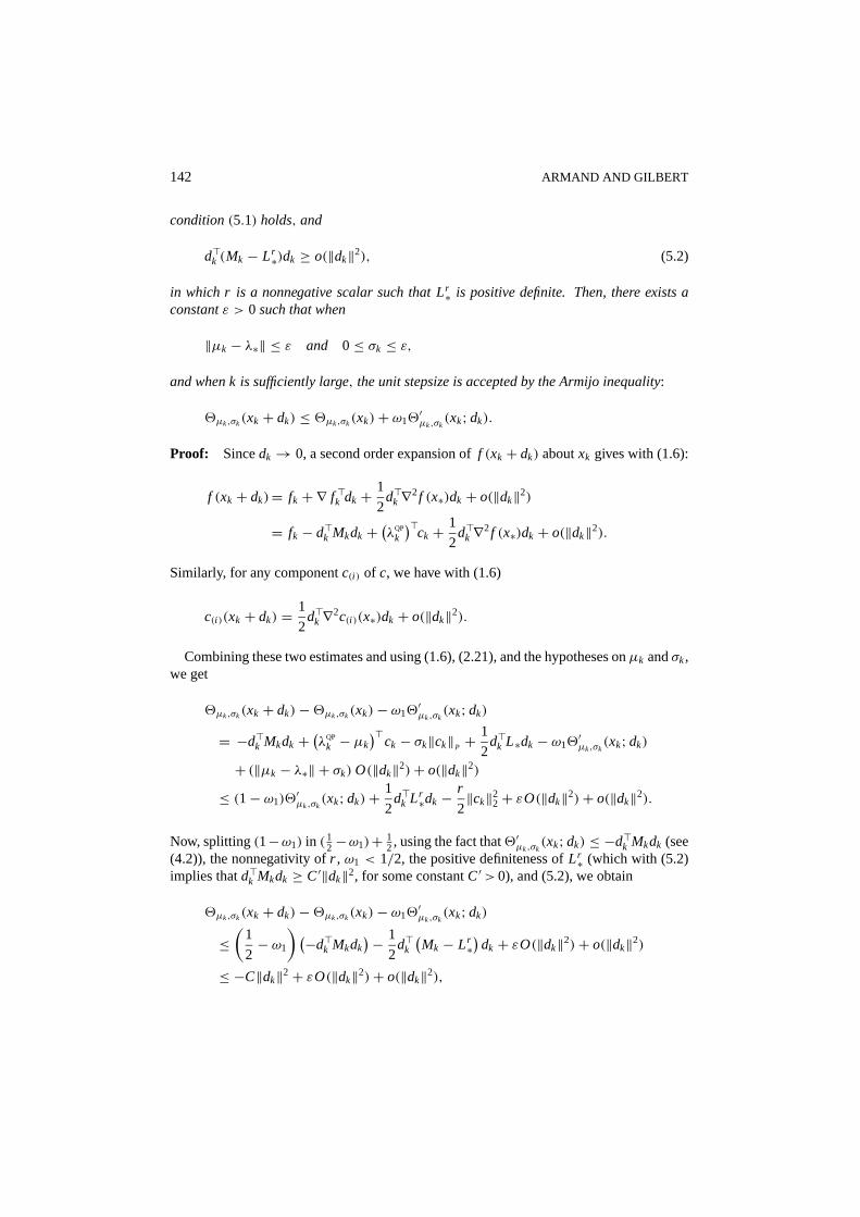
Proposition 5.1. Suppose the f and c are twice continuously differentiable in a convexneighborhood of a local solution x∗ satisfying the second order sufficient condition ofoptimality (1.3)–(1.4). Suppose also that xk → x∗, dk → 0, ω1 < 1/2, the descent
142 ARMAND AND GILBERT
condition(5.1) holds, and
d>k (Mk − Lr∗)dk ≥ o(‖dk‖2), (5.2)
in which r is a nonnegative scalar such that Lr∗ is positive definite. Then, there exists a
constantε > 0 such that when
‖µk − λ∗‖ ≤ ε and 0≤ σk ≤ ε,
and when k is sufficiently large, the unit stepsize is accepted by the Armijo inequality:
2µk,σk(xk + dk) ≤ 2µk,σk(xk)+ ω12′µk,σk
(xk; dk).
Proof: Sincedk → 0, a second order expansion off (xk + dk) aboutxk gives with (1.6):
f (xk + dk)= fk +∇ f >k dk + 1
2d>k∇2f (x∗)dk + o(‖dk‖2)
= fk − d>k Mkdk +(λ
QP
k
)>ck + 1
2d>k∇2f (x∗)dk + o(‖dk‖2).
Similarly, for any componentc(i ) of c, we have with (1.6)
c(i )(xk + dk) = 1
2d>k∇2c(i )(x∗)dk + o(‖dk‖2).
Combining these two estimates and using (1.6), (2.21), and the hypotheses onµk andσk,we get
2µk,σk(xk + dk)−2µk,σk(xk)− ω12′µk,σk
(xk; dk)
= −d>k Mkdk +(λ
QP
k − µk)>
ck − σk‖ck‖P +1
2d>k L∗dk − ω12
′µk,σk
(xk; dk)
+ (‖µk − λ∗‖ + σk)O(‖dk‖2)+ o(‖dk‖2)≤ (1− ω1)2
′µk,σk
(xk; dk)+ 1
2d>k Lr
∗dk − r
2‖ck‖22+ εO(‖dk‖2)+ o(‖dk‖2).
Now, splitting(1−ω1) in ( 12−ω1)+ 1
2, using the fact that2′µk,σk(xk; dk) ≤ −d>k Mkdk (see
(4.2)), the nonnegativity ofr , ω1 < 1/2, the positive definiteness ofLr∗ (which with (5.2)
implies thatd>k Mkdk ≥ C′‖dk‖2, for some constantC′> 0), and (5.2), we obtain
2µk,σk(xk + dk)−2µk,σk(xk)− ω12′µk,σk
(xk; dk)
≤(
1
2− ω1
) (−d>k Mkdk)− 1
2d>k(Mk − Lr
∗)
dk + εO(‖dk‖2)+ o(‖dk‖2)
≤ −C‖dk‖2+ εO(‖dk‖2)+ o(‖dk‖2),
PIECEWISE LINE-SEARCH FOR THE SQP ALGORITHM 143
for some constantC > 0. Since the right hand side is negative whenk is large andε issufficiently small, the proposition is proved. 2
Proposition 5.1 suggests a way of updating the parametersµk, σk, andσ k : µk should beclose toλQP
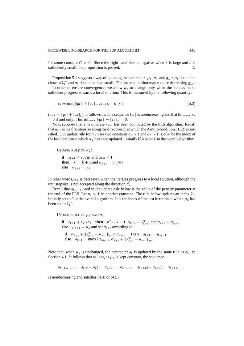
k andσk should be kept small. The latter condition may require decreasingσ k.In order to ensure convergence, we allowµk to change only when the iterates make
sufficient progress towards a local solution. This is measured by the following quantity:
εk = min(‖gk‖ + ‖ck‖P , εk−1), k ≥ 0 (5.3)
(ε−1 = ‖g0‖+‖c0‖P ). It follows that the sequence{εk} is nonincreasing and that limk→∞ εk
= 0 if and only if lim infk→∞ ‖gk‖ + ‖ck‖P = 0.Now, suppose that a new iteratexk+1 has been computed by the PLS algorithm. Recall
thatαk,0 is the first stepsize along the directiondk at which the Armijo condition (3.12) is sat-isfied. Our update rule forσ k uses two constantsa1 > 1 anda2 > 1. Letk′ be the index ofthe last iteration at whichσ k has been updated. Initiallyk′ is set to 0 in the overall algorithm.
UPDATE RULE OFσ k:
if εk+1 ≤ εk′/a1 andαk,0 6= 1then k′ = k+ 1 andσ k+1 = σ k/a2
else σ k+1 = σ k.
In other words,σ k is decreased when the iterates progress to a local solution, although theunit stepsize is not accepted along the directiondk.
Recall thatσk,i k−1 used in the update rule below is the value of the penalty parameter atthe end of the PLS. Leta3 > 1 be another constant. The rule below updates an indexk′′,initially set to 0 in the overall algorithm. It is the index of the last iteration at whichµk hasbeen set toλQP
k .
UPDATE RULE OFµk AND σk:
if εk+1 ≤ εk′′/a3 then k′′ = k+ 1,µk+1 = λQP
k+1, andσk+1 = σ k+1,else µk+1 = µk and setσk+1 according to:
if σ k+1+ ‖λQP
k+1− µk+1‖D ≤ σk,i k−1 then σk+1 = σk,i k−1,else σk+1 = max(2σk,i k−1, σ k+1+ ‖λQP
k+1− µk+1‖D ).
Note that, whenµk is unchanged, the parameterσk is updated by the same rule asσk,i inSection 4.1. It follows that as long asµk is kept constant, the sequence
σk−1,i k−1−1, σk,0(= σk), σk,1, . . . , σk,i k−1, σk+1,0(= σk+1), σk+1,1, . . .
is nondecreasing and satisfies (4.4) or (4.5).
144 ARMAND AND GILBERT
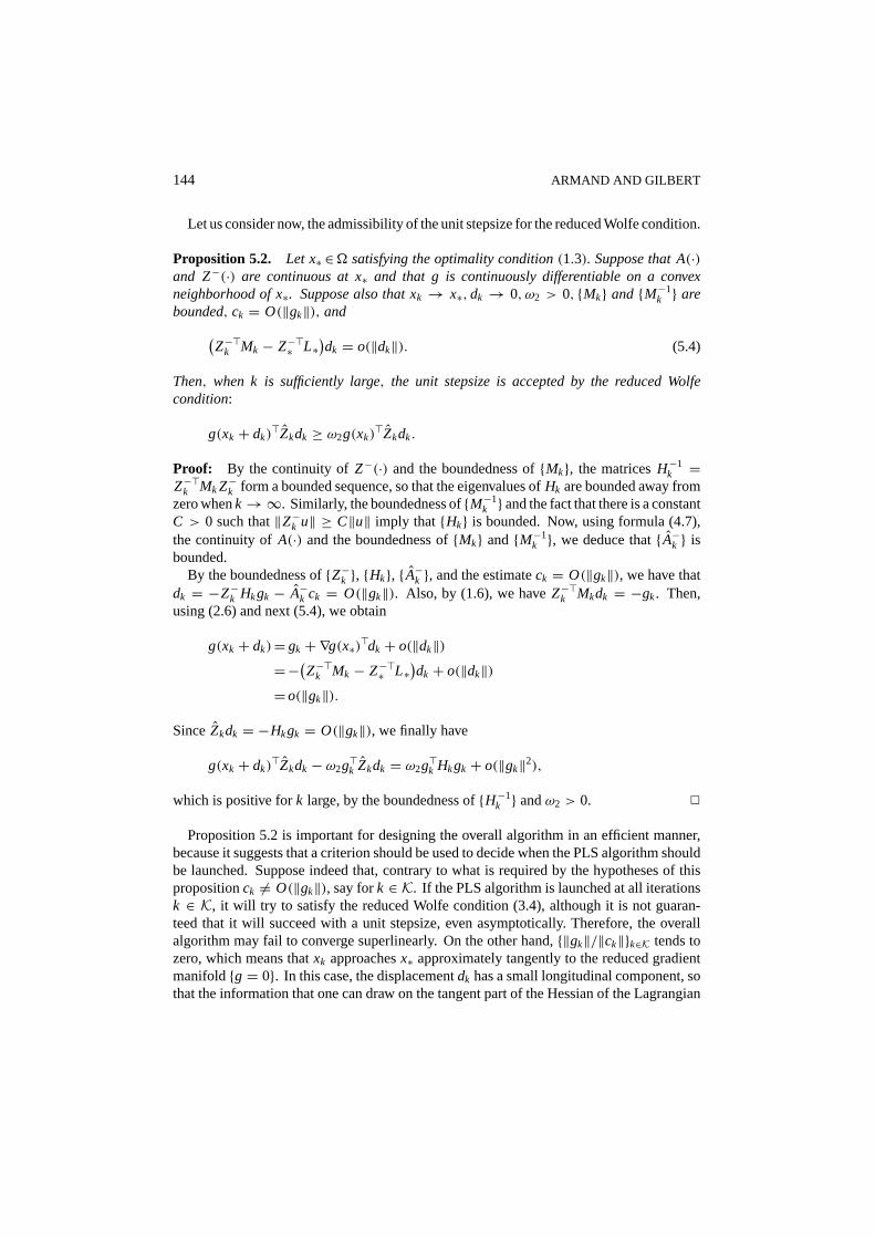
Let us consider now, the admissibility of the unit stepsize for the reduced Wolfe condition.
Proposition 5.2. Let x∗ ∈Ä satisfying the optimality condition(1.3). Suppose that A(·)and Z−(·) are continuous at x∗ and that g is continuously differentiable on a convexneighborhood of x∗. Suppose also that xk → x∗, dk → 0, ω2 > 0, {Mk} and {M−1
k } arebounded, ck = O(‖gk‖), and(
Z−>k Mk − Z−>∗ L∗)dk = o(‖dk‖). (5.4)
Then, when k is sufficiently large, the unit stepsize is accepted by the reduced Wolfecondition:
g(xk + dk)>Zkdk ≥ ω2g(xk)
>Zkdk.
Proof: By the continuity ofZ−(·) and the boundedness of{Mk}, the matricesH−1k =
Z−>k Mk Z−k form a bounded sequence, so that the eigenvalues ofHk are bounded away fromzero whenk→∞. Similarly, the boundedness of{M−1
k } and the fact that there is a constantC > 0 such that‖Z−k u‖ ≥ C‖u‖ imply that {Hk} is bounded. Now, using formula (4.7),the continuity ofA(·) and the boundedness of{Mk} and{M−1
k }, we deduce that{A−k } isbounded.
By the boundedness of{Z−k }, {Hk}, {A−k }, and the estimateck = O(‖gk‖), we have thatdk = −Z−k Hkgk − A−k ck = O(‖gk‖). Also, by (1.6), we haveZ−>k Mkdk = −gk. Then,using (2.6) and next (5.4), we obtain
g(xk + dk)= gk +∇g(x∗)>dk + o(‖dk‖)=−(Z−>k Mk − Z−>∗ L∗
)dk + o(‖dk‖)
= o(‖gk‖).
SinceZkdk = −Hkgk = O(‖gk‖), we finally have
g(xk + dk)>Zkdk − ω2g>k Zkdk = ω2g>k Hkgk + o(‖gk‖2),
which is positive fork large, by the boundedness of{H−1k } andω2 > 0. 2
Proposition 5.2 is important for designing the overall algorithm in an efficient manner,because it suggests that a criterion should be used to decide when the PLS algorithm shouldbe launched. Suppose indeed that, contrary to what is required by the hypotheses of thispropositionck 6= O(‖gk‖), say fork ∈ K. If the PLS algorithm is launched at all iterationsk ∈ K, it will try to satisfy the reduced Wolfe condition (3.4), although it is not guaran-teed that it will succeed with a unit stepsize, even asymptotically. Therefore, the overallalgorithm may fail to converge superlinearly. On the other hand,{‖gk‖/‖ck‖}k∈K tends tozero, which means thatxk approachesx∗ approximately tangently to the reduced gradientmanifold{g = 0}. In this case, the displacementdk has a small longitudinal component, sothat the information that one can draw on the tangent part of the Hessian of the Lagrangian

PIECEWISE LINE-SEARCH FOR THE SQP ALGORITHM 145
is likely to be imprecise. In this case, updatingMk by adjusting the parameterrk only looksperfectly adequate. It is also feasible, sinceck 6= 0 for k ∈ K. These observations suggestnot launching a PLS whenck 6= O(‖gk‖). This leads to the following criterion (K > 0 isa constant).
PLSCRITERION:
if ‖ck‖ ≤ K‖gk‖ then call the PLS algorithm,else perform only the first inner iteration of the PLS algorithm.
It follows that whenever‖ck‖> K‖gk‖, the next iteratexk+1 is set toxk,1, which onlysatisfies condition (3.11) and the Armijo inequality (3.12), but not necessarily the reducedWolfe condition (3.4).
Note finally that the conditions (5.2) and (5.4) on the updated matrixMk, used inPropositions 5.1 and 5.2 are both satisfied when(Mk − Lr
∗)dk = o(‖dk‖), which is areasonable condition to expect from the quasi-Newton theory.
5.2. Global convergence
We are now in position to give a complete description of our BFGS version of the SQPalgorithm.
OVERALL ALGORITHM
0. Choose three constantsai > 1 (i = 1, 2, 3) for the update ofµk, σk, andσ k; aconstantK > 1 for the PLS criterion; and constantsω1 ∈ (0, 1
2), ω2 ∈ (0, 1),andρ ∈ (0, 1
2] for the PLS algorithm.Choose a starting pointx0 ∈ Ä and an initial symmetric positive definite matrixM0 ∈ Rn×n.Setk = k′ = k′′ = 0 (the indicesk′ andk′′ are reset by the update rules ofµk,σk, andσ k).Solve the SQP subproblem (1.5) (withk = 0) giving (d0, λ
QP
0 ).Chooseσ 0 > 0, setµ0 = λQP
0 andσ0 = σ 0.1. if ‖ck‖ ≤ K‖gk‖ then call the PLS algorithm,
else perform only the first inner iteration of the PLS algorithm.This gives a new iteratexk+1.
2. Computeγk andδk by formula (3.2) and (3.14), whererk ≥ 0 is set such thatγ>k δk > 0, and updateMk+1 by the BFGS formula (1.7).
3. Solve the SQP subproblem giving(dk+1, λQP
k+1).4. Updateµk+1, σk+1, andσ k+1 by the rules given in Section 5.1.5. Increasek by 1 and go to 1.
A possible way of determiningrk in Step 2 is described in Section 6.1. Our global con-vergence result below does not require that we specify the update rule ofrk, since its value
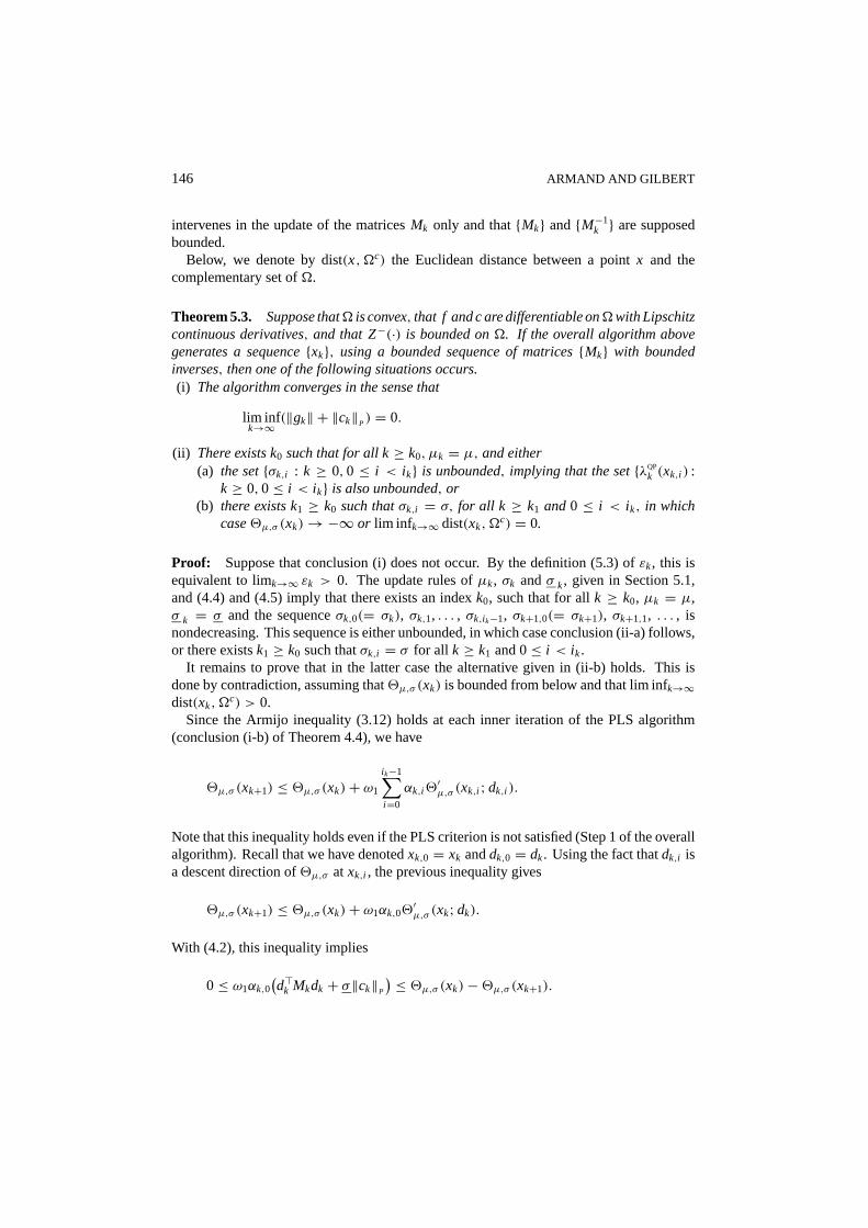
146 ARMAND AND GILBERT
intervenes in the update of the matricesMk only and that{Mk} and{M−1k } are supposed
bounded.Below, we denote by dist(x, Äc) the Euclidean distance between a pointx and the
complementary set ofÄ.
Theorem 5.3. Suppose thatÄ is convex, that f and c are differentiable onÄwith Lipschitzcontinuous derivatives, and that Z−(·) is bounded onÄ. If the overall algorithm abovegenerates a sequence{xk}, using a bounded sequence of matrices{Mk} with boundedinverses, then one of the following situations occurs.(i) The algorithm converges in the sense that
lim infk→∞
(‖gk‖ + ‖ck‖P ) = 0.
(ii) There exists k0 such that for all k≥ k0, µk = µ, and either(a) the set{σk,i : k ≥ 0, 0 ≤ i < i k} is unbounded, implying that the set{λQP
k (xk,i ) :k ≥ 0, 0≤ i < i k} is also unbounded, or
(b) there exists k1 ≥ k0 such thatσk,i = σ, for all k ≥ k1 and0 ≤ i < i k, in whichcase2µ,σ (xk)→−∞ or lim inf k→∞ dist(xk, Ä
c) = 0.
Proof: Suppose that conclusion (i) does not occur. By the definition (5.3) ofεk, this isequivalent to limk→∞ εk > 0. The update rules ofµk, σk andσ k, given in Section 5.1,and (4.4) and (4.5) imply that there exists an indexk0, such that for allk ≥ k0, µk = µ,σ k = σ and the sequenceσk,0(= σk), σk,1, . . . , σk,i k−1, σk+1,0(= σk+1), σk+1,1, . . . , isnondecreasing. This sequence is either unbounded, in which case conclusion (ii-a) follows,or there existsk1 ≥ k0 such thatσk,i = σ for all k ≥ k1 and 0≤ i < i k.
It remains to prove that in the latter case the alternative given in (ii-b) holds. This isdone by contradiction, assuming that2µ,σ (xk) is bounded from below and that lim infk→∞dist(xk, Ä
c) > 0.Since the Armijo inequality (3.12) holds at each inner iteration of the PLS algorithm
(conclusion (i-b) of Theorem 4.4), we have
2µ,σ (xk+1) ≤ 2µ,σ (xk)+ ω1
i k−1∑i=0
αk,i2′µ,σ (xk,i ; dk,i ).
Note that this inequality holds even if the PLS criterion is not satisfied (Step 1 of the overallalgorithm). Recall that we have denotedxk,0 = xk anddk,0 = dk. Using the fact thatdk,i isa descent direction of2µ,σ at xk,i , the previous inequality gives
2µ,σ (xk+1) ≤ 2µ,σ (xk)+ ω1αk,02′µ,σ (xk; dk).
With (4.2), this inequality implies
0≤ ω1αk,0(d>k Mkdk + σ‖ck‖P
) ≤ 2µ,σ (xk)−2µ,σ (xk+1).
PIECEWISE LINE-SEARCH FOR THE SQP ALGORITHM 147
Adding overk and using the boundedness assumption on2µ,σ (xk), we deduce the conver-gence of the series∑
k≥0
αk,0d>k Mkdk <∞ and∑k≥0
αk,0‖ck‖P <∞. (5.5)
If lim inf αk,0 > 0, then the convergence of these series and the boundedness of{M−1k }
would imply thatdk → 0 andck → 0, and sincegk = −Z−>k Mkdk (see (2.16)) we wouldhave(‖gk‖+‖ck‖P )→ 0, in contradiction with our initial assumption. Thus, a subsequence{αk,0}k∈K converges to 0. This means that either condition (3.12) or the Armijo condition(3.12) is not accepted for someα = αk,0, jk ≤ ρ−1αk,0 (Step 1 of the PLS algorithm). Thiscan be written
xk + αk,0, jkdk 6∈ Ä (5.6)
or
2µ,σ (xk + αk,0, jkdk) > 2µ,σ (xk)+ ω1αk,0, jk2′µ,σ (xk; dk). (5.7)
Let us show that (5.6) does not hold for largek. Using the convergence of the firstseries in (5.5), the boundedness of{M−1
k }, andαk,0 ≤ 1, we haveαk,0‖dk‖ → 0. Butfor k ∈ K, αk,0, jk ≤ ρ−1αk,0, so thatαk,0, jk‖dk‖ → 0, which with (5.6) implies thatlim inf dist(xk, Ä
c)→ 0, in contradiction with our assumptions.Now, we show that (5.7) leads to a contradiction, which will prove the theorem. Expand-
ing f andc at the first order and using the Lipschitz continuity of∇ f and∇c, we obtainthe following estimates, whenα ∈ (0, 1] andxk + αdk ∈ Ä:
f (xk + αdk)≤ fk + α∇ f >k dk + Cα2‖dk‖2,µ>c(xk + αdk)≤ (1− α)µ>ck + Cα2‖dk‖2,
and
‖c(xk + αdk)‖P ≤ (1− α)‖ck‖P + Cα2‖dk‖2,
whereC denotes a constant independent ofk. Then,
2µ,σ (xk + αdk)= f (xk + αdk)+ µ>c(xk + αdk)+ σ‖c(xk + αdk)‖P
≤ fk + α∇ f >k dk + (1− α)µ>ck + (1− α)σ‖ck‖P + Cα2‖dk‖2≤2µ,σ (xk)+ α2′µ,σ (xk; dk)+ Cα2‖dk‖2.
The last inequality and (5.7) imply
0< (1− ω1)2′µ,σ (xk; dk)+ Cαk,0, jk‖dk‖2.

148 ARMAND AND GILBERT
Finally, using the inequality2′µ,σ (xk; dk) ≤ −d>k Mkdk − σ‖ck‖P , the boundedness of{M−1
k }, and nextαk,0, jk → 0, whenk→∞ in K, we obtain a contradiction
0< −(1− ω1)σ‖ck‖P − C‖dk‖2 ≤ 0.
This contradiction concludes the proof. 2
Note that in outcome (i) of Theorem 5.3, we only have a subsequence of the iteratesxk, for which‖gk‖ + ‖ck‖P → 0. This is the price that the algorithm pays to allow for adecrease of the penalty parameterσk. A local analysis of the algorithm could show that allthe sequence(ck, gk) actually tends to zero.
We conclude this section by a result specifying the conditions under which the unitstepsize is accepted asymptotically in the overall algorithm.
Proposition 5.4. Let x∗ ∈ Ä satisfying the optimality condition(1.3) and(1.4). Supposethat A(·) and Z−(·) are continuous at x∗ and that f and c are twice continuously differen-tiable and g is continuously differentiable on a convex neighborhood of x∗. If the overallalgorithm generates a sequence{xk} converging to x∗, such that dk → 0, {Mk} and{M−1
k }are bounded, and(Mk − Lr
∗)dk = o(‖dk‖) for some r≥ 0 such that Lr∗ is positive definite.Then, for sufficiently large k, there is only one inner iteration in the PLS algorithm(i.e.,i k = 1) and the unit stepsize is accepted by the Armijo inequality(i.e., αk,0 = 1).
Proof: Sincexk converges to a local solution of the problem, thengk → 0 andck → 0.Thusεk → 0 andλQP
k → λ∗ (use (1.6) andMkdk → 0).Note first thati k = 1 for largek, either because the PLS criterion does not hold or because
of Proposition 5.2.Suppose now thatαk,0 6= 1 for a subsequence of iterates. Then, the update rule ofσ k
implies the convergenceσ k → 0 (it is here that the indexk′ is useful). In the same way,the update rule ofµk andσk impliesµk → λ∗ andσk → 0 (usefulness of the indexk′′). Itfollows from Proposition 5.1 thatαk,0 = 1 for largek, contradicting our initial assumption.
2
This result shows that, under reasonable assumptions, the PLS will finally act like astandard Armijo line-search close to a solution. As a result, this technique is essentiallyuseful away from a solution, where nonconvexity can be encountered.
6. Implementation issues
In this section, we discuss some issues related to the implementation of the algorithmdescribed in the previous sections.
6.1. Computation of rk
Formula (2.10) shows that only the partZ−(x)>Mk of Mk plays a role in the determinationof the SQP direction and that this direction is well defined providedZ−(x)>Mk Z−(x) is
PIECEWISE LINE-SEARCH FOR THE SQP ALGORITHM 149
nonsingular. In this case, because of (2.1), adding a positive multiple ofA>k Ak to Mk doesnot modify the SQP direction. In our case,rk is aimed at forcingMk+1 to approach theHessian of the augmented LagrangianL∗ + rk A>∗ A∗. But since the matrixMk+1 dependsnonlinearly onrk, via the vectorγk and the BFGS formula (1.7), the value ofrk affectsdk+1.This discussion suggests, however, that this value could be set from considerations basedonly on the matrix update.
In the algorithm below, we chooserk in order to minimize an estimate of the conditionnumber of the matrixMk+1. This estimate is the function
ω(M) = tr M
detM1/n
introduced by Dennis and Wolkowicz [13]. Interestingly enough, minimizingω(M) on asubsetS of the set of positive definite matrices is equivalent to minimizing in(ζ,M) ∈(0,+∞) × S the functionψ(ζM), whereψ(M) = tr(M) − ln det(M) is the conditionnumber estimate introduced by Byrd and Nocedal [6]. In both cases, one tries to find thematrix M ∈ S, in a certain sense the closest to the set{ζ I : ζ > 0} of positive definitematrices with unit condition number.
The next proposition analyzes the problem of minimizingω(Mk+1) with respect tork.
Proposition 6.1. Let η, δ, and γ be vectors inRn such thatη>δ > 0 and letγ (r ) =γ + r η, where r is a scalar parameter belonging to the intervalR = {r : γ (r )>δ > 0} =(−γ>δ/η>δ,+∞). Let M be a positive definite matrix and let M(r ) be the matrix obtainedby the BFGS formula, usingγ (r ) andδ:
M(r ) = M − Mδδ>M
δ>Mδ+ γ (r )γ (r )
>
γ (r )>δ.
Then, the function r 7→ ω(M(r )) is uniquely minimized onR by
r = t − γ>δη>δ
, (6.1)
where
t =a+ (a2+ b)12 , a = c1
2(n− 1)c2, b = n+ 1
n− 1
c0
c2, c0 =
∥∥∥∥γ (− γ>δη>δ
)∥∥∥∥2
,
c1= tr M − ‖Mδ‖2
δ>Mδ+ 2
(γ>ηη>δ− ‖η‖2 γ>δ
(η>δ)2
), c2 = ‖η‖
2
(η>δ)2.
Proof: Let us show thatr 7→ ω(M(r )) is pseudoconvex onR, which in particular impliesthat any stationary point is a global minimizer (see [26]). By using
tr M(r ) = tr M − ‖Mδ‖2
δ>Mδ+ ‖γ (r )‖
2
γ (r )>δ
150 ARMAND AND GILBERT
and (see [28])
detM(r ) = γ (r )>δδ>Mδ
detM,
we have trM(r ) = ϕ(γ (r )>δ), whereϕ(t) = c0t +c1+c2t with theci given in the statement
of the proposition. Sincec0 is nonnegative,ϕ is convex on(0,+∞) and, becauser 7→γ (r )>δ is affine, trM(·) is convex onR. On the other hand,M(r ) is positive definite forr ∈ R andr 7→ detM(r ) is affine. Hence the functionω(M(·)) is the quotient of a positiveconvex function and a positive concave function and thus is pseudoconvex onR (see [26,p. 148]).
Now by usingω(M(r )) = ( δ>MδdetM )
1n ω(γ (r )>δ), with ω(t) = t−
1nϕ(t), a straightforward
calculation shows thatt is the unique stationary point ofω(·) on (0,+∞), hencer is theunique global minimum ofω(M(·)) onR. 2
As we said above, settingη = A>k Akδk, δ = δk, andγ = γk = Z>k (gk+1−gk)−A>k (λk+1−λk) in Proposition 6.1, we take in our algorithmrk = r given by formula (6.1). This valueis not defined whenη>k δk = ‖Akδk‖2 = 0. In this case, the discussion in Section 3.4 hasshown that settingrk = 0 is appropriate because the PLS alone ensures the positivity of thescalar productγ>k δk. From a numerical point of view, the difficulty is now to decide when‖Akδk‖ is sufficiently small so thatrk can be set to zero in formula (3.2), while preservingthe positivity ofγ>k δk.
To determine how small‖Akδk‖must be, we compareγ>k δZk to γ>k δ
Ak , whereδZ
k andδAk are
the longitudinal and transversal components ofδk, respectively:
δZk = −αZ
k Z−k Hkgk and δAk = −αA
k A−k ck.
Suppose that the reduced Wolfe condition (3.4) holds. Thenγ>k δZk = αZ
k(gk+1 − gk)>Zkdk
is positive and when
γ>k δAk ≥ −βγ>k δZ
k, (6.2)
for some constantβ ∈ (0, 1), we haveγ>k δk = γ>k δZk + γ>k δA
k ≥ (1− β)γ>k δZk > 0, so that
rk can be set to zero. Therefore, we adopt the following rule for the update ofrk.
COMPUTATION OFrk:
if (3.4) and (6.2) hold then rk = 0,else rk = max(0, rk), whererk is given by (6.1), in whichη = A>k Akδk, δ = δk,andγ = Z>k (gk+1− gk)− A>k (λk+1− λk).
In our numerical experiment, we setβ = 0.1 in (6.2).Sinceγk aims at approximatingL∗δk (see (3.1)), (6.2) may be seen as a way of comparing
the curvatures of the Lagrangian alongδAk and alongδZ
k. The rule above for computingrk canbe read as follows: if the curvature of the Lagrangian in the transversal direction is positive
PIECEWISE LINE-SEARCH FOR THE SQP ALGORITHM 151
or not too negative (with respect to the longitudinal curvature), setrk to zero, otherwise useformula (6.1) to setrk to a positive value. One can also say that (6.2) is a way of measuringthe smallness of‖Akδk‖, since when this quantity vanishes,δA
k = 0 and (6.2) readily holds.
6.2. Using a QR factorization of A>
In our experiment, the matricesA−(x) andZ−(x) described in Section 2 are obtained froma QR factorization ofA(x)>:
A(x)> = (Y−(x) Z−(x) )(
R(x)
0
)= Y−(x)R(x),
whereY−(x) and Z−(x) are respectivelyn × m and n × (n − m) matrices, such that(Y−(x) Z−(x)) is orthogonal, andR(x) is an orderm upper triangular matrix. Clearly,the columns ofZ−(x) span the null space ofA(x), as desired. We choose as right inverseof A(x) the Moore-Penrose pseudo-inverseA(x)>(A(x)A(x)>)−1, which can be computedby
A−(x) = Y−(x)R(x)−>.
With this choice forZ− andA−, it follows thatZ(x) = Z−(x)>.
6.3. Weighted augmentation
Byrd, Tapia and Zhang [8, p. 216] emphasize that, due to the augmentation termA>k Ak inthe vectorγk, badly scaled constraints may have some negative effects on the next updatedmatrix. These authors prefer using a weighted augmentation termA>k Wk Ak, whereWk is anorderm weighting matrix. They suggest usingWk = (Ak A>k )
−1, because with the notationof Section 6.2,
A>k Wk Ak = A>k (Ak A>k )−1Ak = Y−k Y−>k
is a well conditioned matrix.It is clear that the same technique can be adopted in our algorithm. Therefore, in our
experiment we replace the augmentation termA>k Akδk by Y−k Y−>k δk.
6.4. Scaling the tangential direction
It is shown in [20] that the number of inner iterations in the PLS algorithm can be reduced byusing a scaling factorτk,i > 0 on the longitudinal component of the inner search directiondk,i . This leads to redefining the directiondk,i as
dk,i = −τk,i Z−k,i Hkgk − A−k,i ck,i .
152 ARMAND AND GILBERT
For i = 0, we setτk,0 = 1, so that when a unit stepsize is accepted (i k = 1 andαk,0 = 1), aplain SQP step is taken and superlinear convergence of the overall algorithm may occur.
With this change, the vectorδk is still given by (3.14), but the longitudinal stepsizeαZk
has to be computed by
αZk =
i k−1∑i=0
αk,i τk,i .
It is not difficult to extend the finite termination result of Section 4.2 (Theorem 4.4), whendk,i is given as above, providedτk,i is maintained in a fixed interval: 0< τ k ≤ τk,i ≤ τk
for all i ≥ 0. The global convergence result (Theorem 5.3) is not affected by the scalingfactorsτk,i , sinceτk,0 = 1 and only the progress obtained by first inner iteration of the PLSis used in the convergence proof.
6.5. Speeded-up PLS technique
There is another way of speeding up the PLS algorithm that is useful in practice to reducethe number of inner iterations (this is discussed in [20]). It consists in resetting the righthand side of the Wolfe inequality (3.13) toω2g>k,i Zkdk, when the current iteratexk,i makesg>k,i Zkdk more negative than at all the previous inner iterations. Specifically, it consists inreplacing the reduced Wolfe condition (3.4) by the less demanding inequality
g>k+1Zkdk ≥ ω2 min0≤i<i k
g>k,i Zkdk. (6.3)
Since this inequality is more rapidly satisfied than (3.4), the finite termination result(Theorem 4.4) is still valid. Also, the global convergence theorem still holds, since theWolfe condition (3.4) plays no role in its proof.
Let us denote bylk the greatest indexi realizing the minimum in the right hand side of(6.3). When this condition is used in place of (3.4) andlk 6= 0, the vectorsγk andδk haveto be modified. Aiming at havingδk ' xk+1 − xk,lk , the same reasoning as in Sections 3.1and 3.4 shows that it is appropriate to set (we take into account the suggestions given inSections 6.3 and 6.4):
γk= Z>k,lk(gk+1− gk,lk
)− A>k,lk(λk+1− λk,lk
)+ rkY−k,lkY−>k,lkδk
δk=−αZk,lk Z−k,lk Hkgk − αA
k,lk A−k,lkck,lk ,
whereαZk,lk
andαAk,lk
are defined by
αZk,lk =
i k−1∑i=lk
αk,i τk,i and αAk,lk =
i k−1∑i=lk
αk,i e−ξk,i ,
with ξk,i =∑i−1
j=lkαk, j . Note that whenlk = 0 andτk,i = 1, we recover the preceding
formulae (3.2), (3.14), and (3.15).
PIECEWISE LINE-SEARCH FOR THE SQP ALGORITHM 153
Observe finally that whenAk,lkδk = 0, thenck,lk = 0 and we have
γ>k δk= (gk+1− gk,lk)>Zk,lkδk
=αZk,lk(gk+1− gk,lk)
>Zkdk
> 0,
by (6.3). Hence, one can always haveγ>k δk > 0 by adjusting the value ofrk.
7. Numerical experiment
Our experiments were performed on a Power Macintosh 6100/66 in Matlab (release 4.2c.1)with a machine epsilon of about 2× 10⁻¹⁶. We have taken the same list of test problems asin the paper of Byrd, Tapia, and Zhang [8]. In each case, the standard starting points (thosegiven in [25, 33]) were used, except for problems 12, 316–322, 336 and 338, for which wehave usedx0 = 10−4(1, . . . ,1), since the Jacobian matrix is rank deficient at the standardinitial point x0 = 0, which is not supported by our theory.
Three updating methods have been tested:
• Powell : Powell’s corrections, in which, at each iteration,γk is set toγ Pk given by
formula (1.10), withθ calculated as described after this formula (η = 0.1);• BTZ: the Byrd, Tapia, and Zhang approach, in whichγk is given by formula (1.11),
the rules (1.12) and (1.13), withνBTZ = βBTZ = 0.01, and the weighted augmentationdescribed in Section 6.3;• PLS: the algorithm presented in this paper.
All the methods use the same merit function (2.18), with‖·‖P = ‖·‖1, and the sametechnique to update the parametersµ, σ , andσ . The constants, used by the update rules (seeSection 5.1), are set as follows:a1 = 1.0001,a2 = 10,a3 = 1.0001, andσ 0 = ‖λ0‖∞/10.The constant used in the Armijo inequality is set toω1 = 0.01. ForPowell andBTZalgorithms, each stepsizeαk is found by a backtracking line-search alongdk, as in Step 1of the PLS algorithm. In Step 1.2 of the PLS algorithm, quadratic or cubic interpolationformulae are used and we setρ = 0.1. The constant for the reduced Wolfe condition isω2 = 0.9 and the one used in the PLS criterion isK = 100‖c0‖/‖g0‖. Initially, M0 = I andthe pre-update scalingγ>k δk/‖δk‖2I is done before the first update by the BFGS formula.The stopping criterion for all the methods is
‖gk‖2+ ‖ck‖2 ≤ εtol(‖g0‖2+ ‖c0‖2), with εtol = 10−7.
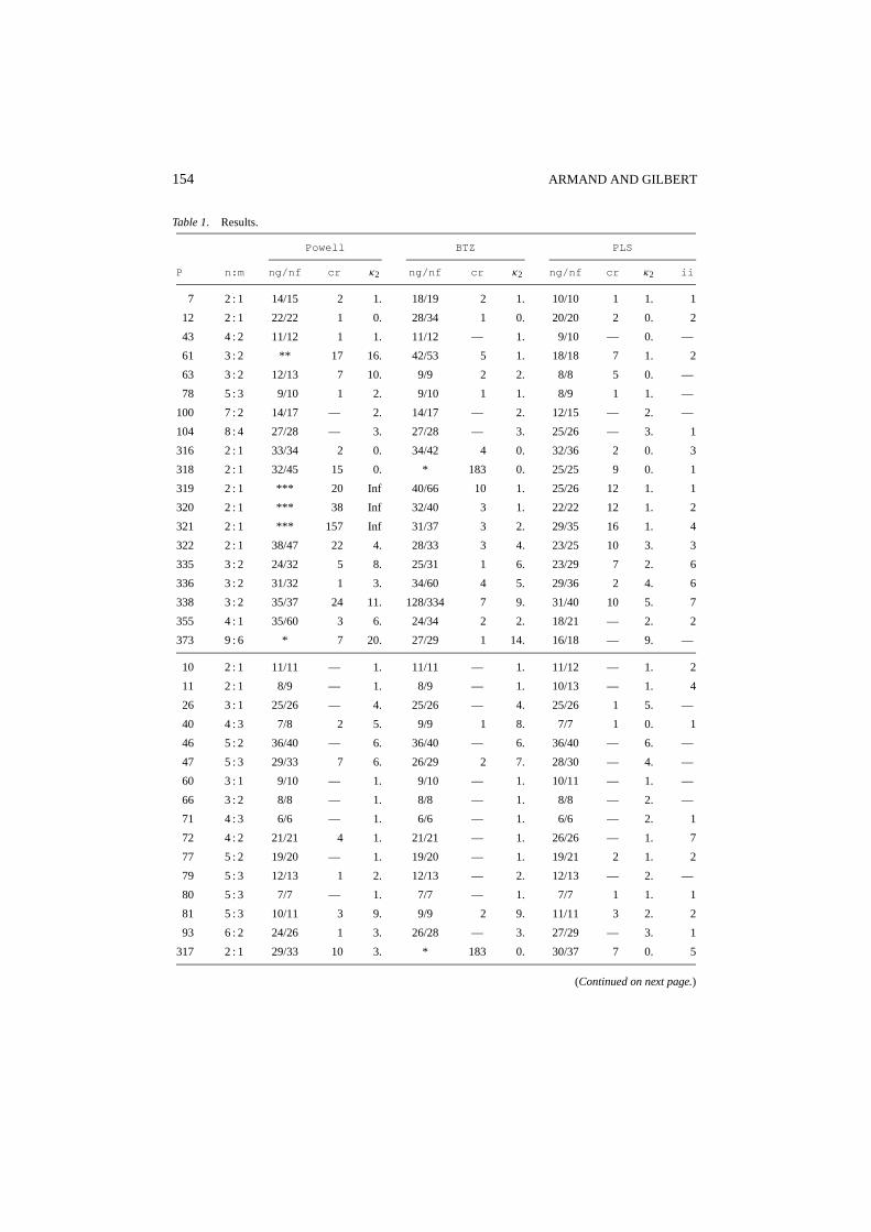
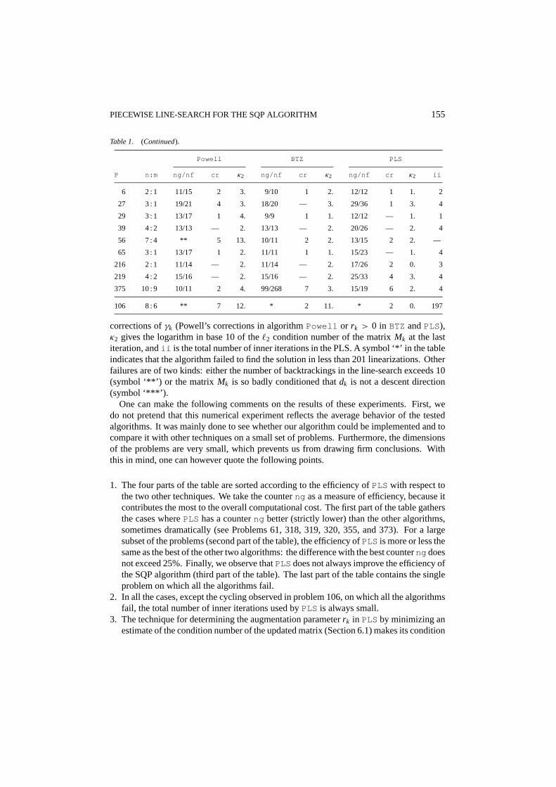
The results are presented in Table 1. The columns in this table are labeled as follows:P is the problem number given in [25, 33],n is the number of variables,m is the numberof constraints,ng is the number of gradient calculations and constraint linearizations (themain computation cost),nf is the number of function evaluations,cr is the number of
154 ARMAND AND GILBERT
Table 1. Results.
Powell BTZ PLS
P n:m ng/nf cr κ2 ng/nf cr κ2 ng/nf cr κ2 ii
7 2 : 1 14/15 2 1. 18/19 2 1. 10/10 1 1. 1
12 2 : 1 22/22 1 0. 28/34 1 0. 20/20 2 0. 2
43 4 : 2 11/12 1 1. 11/12 — 1. 9/10 — 0. —
61 3 : 2 ** 17 16. 42/53 5 1. 18/18 7 1. 2
63 3 : 2 12/13 7 10. 9/9 2 2. 8/8 5 0. —
78 5 : 3 9/10 1 2. 9/10 1 1. 8/9 1 1. —
100 7 : 2 14/17 — 2. 14/17 — 2. 12/15 — 2. —
104 8 : 4 27/28 — 3. 27/28 — 3. 25/26 — 3. 1
316 2 : 1 33/34 2 0. 34/42 4 0. 32/36 2 0. 3
318 2 : 1 32/45 15 0. * 183 0. 25/25 9 0. 1
319 2 : 1 *** 20 Inf 40/66 10 1. 25/26 12 1. 1
320 2 : 1 *** 38 Inf 32/40 3 1. 22/22 12 1. 2
321 2 : 1 *** 157 Inf 31/37 3 2. 29/35 16 1. 4
322 2 : 1 38/47 22 4. 28/33 3 4. 23/25 10 3. 3
335 3 : 2 24/32 5 8. 25/31 1 6. 23/29 7 2. 6
336 3 : 2 31/32 1 3. 34/60 4 5. 29/36 2 4. 6
338 3 : 2 35/37 24 11. 128/334 7 9. 31/40 10 5. 7
355 4 : 1 35/60 3 6. 24/34 2 2. 18/21 — 2. 2
373 9 : 6 * 7 20. 27/29 1 14. 16/18 — 9. —
10 2 : 1 11/11 — 1. 11/11 — 1. 11/12 — 1. 2
11 2 : 1 8/9 — 1. 8/9 — 1. 10/13 — 1. 4
26 3 : 1 25/26 — 4. 25/26 — 4. 25/26 1 5. —
40 4 : 3 7/8 2 5. 9/9 1 8. 7/7 1 0. 1
46 5 : 2 36/40 — 6. 36/40 — 6. 36/40 — 6. —
47 5 : 3 29/33 7 6. 26/29 2 7. 28/30 — 4. —
60 3 : 1 9/10 — 1. 9/10 — 1. 10/11 — 1. —
66 3 : 2 8/8 — 1. 8/8 — 1. 8/8 — 2. —
71 4 : 3 6/6 — 1. 6/6 — 1. 6/6 — 2. 1
72 4 : 2 21/21 4 1. 21/21 — 1. 26/26 — 1. 7
77 5 : 2 19/20 — 1. 19/20 — 1. 19/21 2 1. 2
79 5 : 3 12/13 1 2. 12/13 — 2. 12/13 — 2. —
80 5 : 3 7/7 — 1. 7/7 — 1. 7/7 1 1. 1
81 5 : 3 10/11 3 9. 9/9 2 9. 11/11 3 2. 2
93 6 : 2 24/26 1 3. 26/28 — 3. 27/29 — 3. 1
317 2 : 1 29/33 10 3. * 183 0. 30/37 7 0. 5
(Continued on next page.)
PIECEWISE LINE-SEARCH FOR THE SQP ALGORITHM 155
Table 1. (Continued).
Powell BTZ PLS
P n:m ng/nf cr κ2 ng/nf cr κ2 ng/nf cr κ2 ii
6 2 : 1 11/15 2 3. 9/10 1 2. 12/12 1 1. 2
27 3 : 1 19/21 4 3. 18/20 — 3. 29/36 1 3. 4
29 3 : 1 13/17 1 4. 9/9 1 1. 12/12 — 1. 1
39 4 : 2 13/13 — 2. 13/13 — 2. 20/26 — 2. 4
56 7 : 4 ** 5 13. 10/11 2 2. 13/15 2 2. —
65 3 : 1 13/17 1 2. 11/11 1 1. 15/23 — 1. 4
216 2 : 1 11/14 — 2. 11/14 — 2. 17/26 2 0. 3
219 4 : 2 15/16 — 2. 15/16 — 2. 25/33 4 3. 4
375 10 : 9 10/11 2 4. 99/268 7 3. 15/19 6 2. 4
106 8 : 6 ** 7 12. * 2 11. * 2 0. 197
corrections ofγk (Powell’s corrections in algorithmPowell or rk > 0 in BTZ andPLS),κ2 gives the logarithm in base 10 of the`2 condition number of the matrixMk at the lastiteration, andii is the total number of inner iterations in the PLS. A symbol ‘*’ in the tableindicates that the algorithm failed to find the solution in less than 201 linearizations. Otherfailures are of two kinds: either the number of backtrackings in the line-search exceeds 10(symbol ‘**’) or the matrix Mk is so badly conditioned thatdk is not a descent direction(symbol ‘***’).
One can make the following comments on the results of these experiments. First, wedo not pretend that this numerical experiment reflects the average behavior of the testedalgorithms. It was mainly done to see whether our algorithm could be implemented and tocompare it with other techniques on a small set of problems. Furthermore, the dimensionsof the problems are very small, which prevents us from drawing firm conclusions. Withthis in mind, one can however quote the following points.
1. The four parts of the table are sorted according to the efficiency ofPLS with respect tothe two other techniques. We take the counterng as a measure of efficiency, because itcontributes the most to the overall computational cost. The first part of the table gathersthe cases wherePLS has a counterng better (strictly lower) than the other algorithms,sometimes dramatically (see Problems 61, 318, 319, 320, 355, and 373). For a largesubset of the problems (second part of the table), the efficiency ofPLS is more or less thesame as the best of the other two algorithms: the difference with the best counterng doesnot exceed 25%. Finally, we observe thatPLSdoes not always improve the efficiency ofthe SQP algorithm (third part of the table). The last part of the table contains the singleproblem on which all the algorithms fail.
2. In all the cases, except the cycling observed in problem 106, on which all the algorithmsfail, the total number of inner iterations used byPLS is always small.
3. The technique for determining the augmentation parameterrk in PLS by minimizing anestimate of the condition number of the updated matrix (Section 6.1) makes its condition
156 ARMAND AND GILBERT
number smaller inPLS than in the other algorithms. This technique could also be usedfor algorithmBTZ. In order to make a clear comparison betweenBTZ andPLS we alsoran the former using formula (6.1) of Proposition 6.1 for the computation ofrk. Moreprecisely, we setrk = max(rk, r BTZ
k ), whererk is the value given by (6.1) andr BTZk is
the one given by formula (1.12). Curiously, we did not observe an improvement on thecountersng andnf on average, though the condition number of the matricesMk at thelast iteration were better than those given in Table 1.
4. Finally, regarding the usual counters (ng and nf ), there is no clear winner.PLS isthe most efficient on 42% of the test problems (first part of the table), one of the mostefficient on 36% of the test problems (second part of the table) and not the most efficienton the other problems. On the other hand,PLS is more robust in that it fails less oftenthanPowell or BTZ.
8. Conclusion
This paper proposes a technique for maintaining the positive definiteness of the updatedmatrices in the quasi-Newton version of the SQP algorithm for equality constrained op-timization problems. The overall algorithm generates approximations of the Hessian ofthe augmented Lagrangian, whose positive definiteness is obtained via the realization ofa reduced Wolfe condition and an adequate setting of the augmentation parameter. Theglobalization is obtained by means of a nondifferentiable augmented Lagrangian functionas merit function. Finite termination of the search algorithm, global convergence (assumingboundedness of the generated matrices and their inverses) and asymptotic admissibility ofthe unit stepsize are proved.
What is new in the proposed approach is the use of a piecewise line-search algorithm,mimicking what is done for unconstrained problems. To tell it vaguely, this algorithmensures the positive definiteness of the matrices in the space tangent to the constraints. Webelieve that this is a conceptual improvement on the algorithm proposed by Byrd, Tapia,and Zhang [8], with which our method has similarities.
The numerical experiment indicates that the proposed algorithm can be more robust thanexisting approaches, although there is not a uniform improvement on the usual counters.
Finally, not all the facets of the algorithm have been studied. It is hoped that a preciseanalysis of the possibility to have superlinear convergence of the method (such as in thepapers [8] and [19]) may improve the algorithm. We plan to undertake this study.
Acknowledgments
We would like to thank Richard Byrd and Jorge Nocedal for an exciting discussion at anearly stage of the design of the algorithm, which has certainly influence our point of viewon the implementation of the PLS technique for the SQP method.
References
1. L.T. Biegler, J. Nocedal, and C. Schmid, “A reduced Hessian method for large-scale constrained optimization,”SIAM Journal on Optimization,” vol. 5, pp. 314–347, 1995.
PIECEWISE LINE-SEARCH FOR THE SQP ALGORITHM 157
2. P.T. Boggs and J.W. Tolle, “Sequential quadratic programming,” in Acta Numerica 1995, Cambridge Univer-sity Press, pp. 1–51, 1995.
3. J.F. Bonnans, “Asymptotic admissibility of the unit stepsize in exact penalty methods,” SIAM Journal onControl and Optimization, vol. 27, pp. 631–641, 1989.
4. J.F. Bonnans, J.Ch. Gilbert, C. Lemar´echal, and C. Sagastiz´abal, Mathematiques et Applications, vol. 27:Optimisation Num´erique—Aspects th´eoriques et pratiques, Springer Verlag: Berlin, 1997.
5. R.H. Byrd, J.Ch. Gilbert, and J. Nocedal, “A trust region method based on interior point techniques fornonlinear programming,” Rapport de Recherche 2896, INRIA, 1996. (Submitted to Mathematical Pro-gramming)
6. R.H. Byrd and J. Nocedal, “A tool for the analysis of quasi-Newton methods with application to unconstrainedminimization,” SIAM Journal on Numerical Analysis, vol. 26, pp. 727–739, 1989.
7. R.H. Byrd and J. Nocedal, “An analysis of reduced Hessian methods for constrained optimization,” Mathe-matical Programming, vol. 49, pp. 285–323, 1991.
8. R.H. Byrd, R.A. Tapia, and Y. Zhang, “An SQP augmented Lagrangian BFGS algorithm for constrainedoptimization,” SIAM Journal on Optimization, vol. 2, pp. 210–241, 1992.
9. F.H. Clarke, Optimization and Nonsmooth Analysis, John Wiley & Sons: New York, 1983.10. T.F. Coleman and A.R. Conn, “On the local convergence of a quasi-Newton method for the nonlinear pro-
gramming problem,” SIAM Journal on Numerical Analysis, vol. 21, pp. 755–769, 1984.11. T.F. Coleman and P.A. Fenyes, “Partitioned quasi-Newton methods for nonlinear constrained optimization,”
Mathematical Programming, vol. 53, pp. 17–44, 1992.12. J.E. Dennis and R.B. Schnabel, Numerical Methods for Unconstrained Optimization and Nonlinear Equations,
Prentice-Hall: Englewood Cliffs, 1983.13. J.E. Dennis and H. Wolkowicz, “Sizing and least-change secant methods,” SIAM Journal on Numerical
Analysis, vol. 30, pp. 1291–1314, 1993.14. R. Fletcher, Practical Methods of Optimization, 2nd ed., John Wiley & Sons: Chichester, 1987.15. D. Gabay, “Minimizing a differentiable function over a differential manifold,” Journal of Optimization Theory
and Applications, vol. 37, pp. 177–219, 1982.16. D. Gabay, “Reduced quasi-Newton methods with feasibility improvement for nonlinearly constrained opti-
mization,” Mathematical Programming Study, vol. 16, pp. 18–44, 1982.17. J.Ch. Gilbert, “Mise `a jour de la m´etrique dans les m´ethodes de quasi-Newton r´eduites en optimisation
avec contraintes d’´egalite,” Modelisation Mathematique et Analyse Num´erique, vol. 22, pp. 251–288,1988.
18. J.Ch. Gilbert, “Maintaining the positive definiteness of the matrices in reduced secant methods for equalityconstrained optimization,” Mathematical Programming, vol. 50, pp. 1–28, 1991.
19. J.Ch. Gilbert, “Superlinear convergence of a reduced BFGS method with piecewise line-search and up-date criterion,” Rapport de Recherche 2140, INRIA, BP 105, 78153 Le Chesnay, France, 1993.http://www.inria.fr/RRRT/RR-2140.html; ftp://ftp.inria.fr/INRIA/publication/RR, RR-2140.ps.gz.
20. J.Ch. Gilbert, “On the realization of the Wolfe conditions in reduced quasi-Newton methods for equalityconstrained optimization,” SIAM Journal on Optimization, vol. 7, pp. 780–813, 1997.
21. C.B. Gurwitz, “Local convergence of a two-piece update of a projected Hessian matrix,” SIAM Journal onOptimization, vol. 4, pp. 461–485, 1994.
22. S.-P. Han, “Superlinearly convergent variable metric algorithms for general nonlinear programming problems,”Mathematical Programming, vol. 11, pp. 263–282, 1976.
23. S.-P. Han and O.L. Mangasarian, “Exact penalty functions in nonlinear programming,” Mathematical Pro-gramming, vol. 17, pp. 251–269, 1979.
24. J.-B. Hiriart-Urruty and C. Lemar´echal, Convex Analysis and Minimization Algorithms, Springer-Verlag,1993, Grundlehren der mathematischen Wissenschaften 305–306.
25. W. Hock and K. Schittkowski, Lecture Notes in Economics and Mathematical Systems, vol. 187: TestExamples for Nonlinear Programming Codes, Springer-Verlag: Berlin, 1981.
26. O.L. Mangasarian, Nonlinear Programming, McGraw-Hill: New York, 1969.27. J. Nocedal and M.L. Overton, “Projected Hessian updating algorithms for nonlinearly constrained optimiza-
tion,” SIAM Journal on Numerical Analysis, vol. 22, pp. 821–850, 1985.

158 ARMAND AND GILBERT
28. J.D. Pearson, “Variable metric methods of minimization,” The Computer Journal, vol. 12, pp. 171–178, 1969.29. M.J.D. Powell, “The convergence of variable metric methods for nonlinearly constrained optimization cal-
culations,” in Nonlinear Programming, vol. 3, O.L. Mangasarian, R.R. Meyer, and S.M. Robinson (Eds.),Academic Press: New York, 1978, pp. 27–63.
30. M.J.D. Powell, “A fast algorithm for nonlinearly constrained optimization calculations,” in Lecture Notes inMathematics, vol. 630: Numerical Analysis Dundee 1977, G.A. Watson (Ed.), Springer-Verlag: Berlin, 1978,pp. 144–157.
31. M.J.D. Powell, “The performance of two subroutines for constrained optimization on some difficult test prob-lems,” in Numerical Optimization 1984, P.T. Boggs, R.H. Byrd, and R.B. Schnabel (Eds.), SIAM Publication:Philadelphia, 1985, pp. 160–177.
32. M.J.D. Powell, “A view of nonlinear optimization,” in History of Mathematical Programming, A Collectionof Personal Reminiscences, J.K. Lenstra, A.H.G. Rinnooy Kan, and A. Schrijver (Eds.), CWI North-Holland:Amsterdam, 1991, pp. 119–125.
33. K. Schittkowski, Lecture Notes in Economics and Mathematical Systems, vol. 282: More Test Examples forNonlinear Programming Codes, Springer-Verlag, 1987.
34. L. Schwartz, Analyse II—Calcul Diff´erentiel etEquations Differentielles, Hermann, Paris, 1992.35. R.A. Tapia, “Diagonalized multiplier methods and quasi-Newton methods for constrained optimization,”
Journal of Optimization Theory and Applications, vol. 22, pp. 135–194, 1977.36. R.A. Tapia, “On secant updates for use in general constrained optimization,” Mathematics of Computation,
vol. 51, pp. 181–202, 1988.37. P. Wolfe, “Convergence conditions for ascent methods,” SIAM Review, vol. 11, pp. 226–235, 1969.38. P. Wolfe, “Convergence conditions for ascent methods II: Some corrections,”SIAM Review, vol. 13, pp. 185–
188, 1971.39. Y. Xie and R.H. Byrd “Practical update criteria for reduced Hessian SQP: global analysis,”SIAM Journal on
Optimization, vol. 9, pp. 578–604, 1999.