A Perturbation/Correlation Approachto Force-Guided Robot Control

by

Sooyong Lee

B.S.M.E. Seoul National University, Seoul, KOREA, 1989

M.S.M.E. Seoul National University, Seoul, KOREA, 1991

Submitted to the Department of Mechanical Engineeringin Partial Fulfillment of the Requirements for the Degree of

DOCTOR OF PHILOSOPHY

at the

MASSACHUSETTS INSTITUTE OF TECHNOLOGY

JUNE 1996

Copyright. Massachusetts Institute of Technology 1996All rights reserved

Signature of AuthorC Depaftment of Mechanical Engineering

May 14, 1996

Certified by ,,t . , ,Haruhiko Asada

Professor of Mechanical EngineeringThesis Supervisor

Accepted by

O rFCH " 'O

JUN 2 7 1996

Ain A. SoninChairman, Department Committee on Graduate Students

a&i

Upr

V

A Perturbation/Correlation Approachto Force-Guided Robot Control

Sooyong Lee

Abstract

Force guided robot control is a control scheme based on the interpretation of measuredforce acting on the robot end effector. A functional map relating the correction of motion toforce measurements is generated based on the geometry of the workpiece and its kinematicbehavior in interacting with the environment. In the traditional force-guided controlschemes, the contact force measured by a force sensor is directly fed back to a feedbackcontroller to generate a motion correction signal. However, the force information obtainedat one point does not always contain sufficient information to determine the direction ofmotion. The forces measured are often erratic and noisy due to the friction at the contactingsurfaces and the existence of irregular burrs. This often leads to a misjudgment of contactconfigurations and erratic control actions. Also, the erratic force feedback may lead toexcessive contact forces and large friction, which impede smooth motion and incurjamming and damage to the objects. Therefore, it is important to maintain the contact forceat an appropriate level. The issue central to force guided robot control is how to obtainreliable, consistent and copious force signals and extract useful information in order tosuccessfully guide the robot while keeping the contact force at a desired level.

In this thesis, instead of simply measuring contact forces, we take positive actions bygiving perturbation to the end effector and observing the reaction forces to the perturbationin order to obtain much richer and more reliable information. By taking the correlationbetween the input perturbation and the resultant reaction forces, we can determine thegradient of the force profile and guide the part correctly. By applying a type of directadaptive control, the contact force is maintained at the lowest level. This algorithm isapplied to a pipe insertion task, in which the insertion force is minimized during theinsertion. Based on the process model and stability analysis using the Popov stabilitycriterion, conditions for stable, successful insertion despite nonlinearities and uncertaintiesin the environment are obtained. The theoretical results are verified using the experimentaldata. To generate high frequency perturbation, a vibratory end effector using piezoelectricactuators is designed and built. Also, this perturbation/correlation method is applied to abox palletizing task, in which a rectangular box is to be located in one corner of the wallwhile maintaining constant contact with the wall. Through both simulations andexperiments, the feasibility and usefulness of these methods are demonstrated.

Thesis Committee :

Haruhiko Asada Professor, Mechanical EngineeringKamal Youcef-Toumi Professor, Mechanical EngineeringFrank Feng Professor, Mechanical Engineering

Contents

1 Introduction

1.1 Issues and Previous Work . .................. .... 8

1.2 Objectives and Outline of the Thesis . ................. 11

2 Control Architecture

2.1 Introduction . . . . . . . . . . . . . . . . . . . . . . . . . . . . . .14

2.2 Perturbation/Correlation ................... ..... 14

2.3 Application to the Force Guided Robot . ................ 19

3 Case Study : Pipe Insertion Task

3.1 Introduction . . . . . . . . . . . . . . . . . . . . . . . . . . . . . .27

3.2 Pipe Insertion Task .......................... 27

3.3 Modeling of the Process ........................ 31

3.4 Selection of Parameters ........................ 35

3.5 Simulation . . . . . . . . . . . . . . . . . . . . . . . . . . . . . . 37

3.6 Extension to Three Dimension ................... .. 38

4. Stability Analysis

4.1 Introduction . ................. . .. .... .... .. 42

4.2 Linear System . ............... ... . .. .. ... .. 42

4.3 Nonlinear and Unknown System ................... . 44

4.4 Simulation . . . . . . . . . . . . . . . . . . . . . . . . . . .. . . . 50

5 Experiment and Implementation

5.1 Introduction . . . . . . . . . . . . . . . . . . . . . . . . . . . . . . 54

5.2 Vibratory End Effector using Piezo Electric Actuator ....... . . . . . 54

5.3 Experimental Setup .......................... 57

5.4 Experimental Data ....................... .... 59

5.5 Comparison with Other Force-Guided Controller . ........... 61

5.6 Friction Reduction Due to Perturbation . ................ 63

6. Application to the Connector Assembly Task

6.1 Introduction . . . . . . . . . . . . . . . . . . . . . . . . . . . . . . 67

6.2 Connector Assembly ................. ......... 67

6.3 Modeling .. ............ ................. 69

6.4 Perturbation/Correlation based Control . . . . . . . . . . . . . . . . . 73

6.5 Sim ulation . . . . . . . . . . . . . . . . . . . . . . . . . . . . . . . 76

6.6 Comparison with Pipe Insertion Task ........... . . . . . . 78

7. Conclusion

7.1 Contributions . . . . . . . . . . . . . . . . . . . . . . . . . . . . . 80

7.2 Further W ork . . . . . . . . . . . . . . . . . . .... . . . .. . . . 81

Reference

List of Figures

Figure 1-1. Force guided control .. ...... .. ......... ....... 8

Figure 1-2. Symmetric position-force relationship . . ........... . . ..... 10

Figure 2-1. Performance index F and input p . .. . . . . . ... . . . . . . . . . 15

Figure 2-2. Perturbation Method .......................... 16

Figure 2-3. Linear Regression .... ....... ....... ... ...... 16

Figure 2-4. Time-Varying System ........... ............... 18

Figure 2-5. Robot with Environment ........................ 20

Figure 2-6. Robot Dynamics ............................ 20

Figure 2-7. Robot with Position Controller . . . . . . . . . . . . . . . . . . . . 20

Figure 2-8. Simplified Representation ... ...... . ... . . . . . . . . . . 21

Figure 2-9. Performance Index .... ...... ........ .... ... . 21

Figure 2-10. Perturbation/Correlation . . . . . . . . . . . . . . . . . .. . . . . 21

Figure 2-11. Gradient of the Performance Index . ................. 22

Figure 2-12. Robot System with Perturbation/Correlation . ............. 24

Figure 2-13. System with Linear and Nonlinear Block . . . . . . . . . . . . . . . 25

Figure 2-14. Implementation of the Controller . . . . . . . . . . . . ... . . . . 26

Figure 3-1. Pipe insertion task ........................... 28

Figure 3-2. Obstructing force Fz v.s. displacement x . . ........... . . . . . . 29

Figure 3-3. Robot with Perturbation/Correlation ............. ..... . . . . . 30

Figure 3-4 Insertion force varies depending on x, z and . . . . . ..... . . . . . . 31

Figure 3-5. Experimental Setup ............................ 32

Figure 3-6. FZ as a function of x and z ..... ........... ....... 33

Figure 3-7. F, as a function of z and i ....................... 33

Figure 3-8. System modeling ........................... 34

Figure 3-9. Block diagram representation . .................. . . .34

Figure 3-10. Simulation Result .......................... 38

Figure 3-11. End Effector Trajectory . . . . . . . . . . . . . . . . . . . . . . . 41

Figure 3-12. Performance Index Time History . . . . . . . . . . . . . . . . . . . 41

Figure 4-1. Block diagram representation . . . . . . . . . . . . . . . . . . . ...... 43

Figure 4-2. System with nonlinearity ... . . . . . . . .... . . . . . . . . . 45

Figure 4-3. Nonlinearity ..................... ... .... . 46

Figure 4-4. Displacement vs. Force ......... . . . . . . . . . . . . . . . 46

Figure 4-5. Plot of transfer function ................ ......... 49

Figure 4-6. Simulation Results for Linear Case . . . . .. . . . . . . . . . . . .....52

Figure 4-7. Nonlinear Force Function . . . . . . . . . . . . . . . . . . . . . . . 52

Figure 4-8. Simulation Results for Nonlinear Case . . . . . . . . . . . . . . . . . 53

Figure 5-1. Vibratory Endeffector ......................... 55

Figure 5-2. Isolated view of the End Effector Head . . . . . . . . . . . . . . . . . 55

Figure 5-3. Movement of the End Effector . . . . . . . . . . . . . . . . . . . . . 56

Figure 5-4. Vibratory End Effector with Piezo Electric Actuators . . . . . . . . . . 56

Figure 5-5. Vibratory End Effector Mounted on a Force Sensor . . . . . . . . . . . 57

Figure 5-6. Experimental Setup .......................... 58

Figure 5-7. Pipe Insertion by Robot ........................ 58

Figure 5-8. Experimental Data ........................... 59

Figure 5-9. Verification of the Eq (5-1) . .................. . . . 60

Figure 5-10. Compliance Center .......................... 61

Figure 5-11. X-displacement and Force Response of the Robot Dither Case . . . . . 62

Figure 5-12. Comparison with Conventional Controller . . . . . . . . . . . . . . . 63

Figure 5-13. Experiment Setup ................ ........... . 64

Figure 5-14. Force Profile with Perturbation . . . . . . . . . . . . . . . . . . . . 65

Figure 5-15. Resistant Force Comparison ................... .. 66

Figure 6-1. Connector Assembly ............. ............ 68

Figure 6-2. Reaction Forces ........................... 70

Figure 6-3. Coordinates . . .. ... . ... . ... . .. .. .. . .. . .. . 71

Figure 6-4. Contact Points of the Box ....................... 72

Figure 6-5. Performance Index, X, Y, and Theta ............. . . . 77

Figure 6-6. Movement of the Connector ................... ... 78

Chapter 1

Introduction

1.1 Issues and Previous Work

Force guided robot control is a control scheme based on a stored map from forces to

a correction of motion. As shown in Figure 1-1, the motion command is generated through

the interpretation of the measured force at the block termed, the "force-to-motion map".

Based on the geometry of the workpiece and its kinematic behavior in interacting with the

environment, the functional map relating the correction of motion to force measurements is

generated. In the past, various methods for designing this map have been developed.

[Hanafusa, Asada, 1977], [Whitney, 1977], [Peshikin, 1992]

ReferenceForceProfile

Figure 1-1. Force guided control

The force feedback law may be a simple compliance control law, an admittance control

law, or a complex nonlinear control law described by a functional relationship between

motion correction signals and the measured force, position, and velocity signals. For more

complex tasks, the block of force feedback law may include a logical branch controller and

a process monitor, which detects contact changes and determines contact configurations

during the operation [Whitney, 1987]. Based on the estimated contact configuration, the

correction of robot motion is generated for the robot control system [McCarragher, Asada,

1993]. In any case, the feedback law in the traditional force-guided assembly is

represented by a map from measured forces and state variables to a motion correction

command. It should be noted that the controller simply receives the force signals generated

in the assembly process, which are often erratic and noisy.

To improve the reliability and assure assembly operations, in-process monitoring and

closed-loop process control are powerful tools. For monitoring an assembly process, the

force and moment acting between mating parts are the major sources of information directly

related to the assembly process state. Unlike visual information, the force information

provides real-time, in-process information during parts mating operations. Therefore, the

force information is indispensable for closed-loop assembly process control as well as for

in-process monitoring. To make robotic assembly reliable and robust in the face of a high

degree of uncertainties, the closed loop control based on force information and in-process

monitoring is critically important. The question is how to obtain useful force information

despite inherent difficulties.

Although force information is useful and even indispensable in performing a task that

involves mechanical contacts and interactions with the environment, the control based on

the simple force-to-motion map, sometimes incurs unwanted behavior. One of the

problems often encountered in force guided robot control is "undecidable" situations

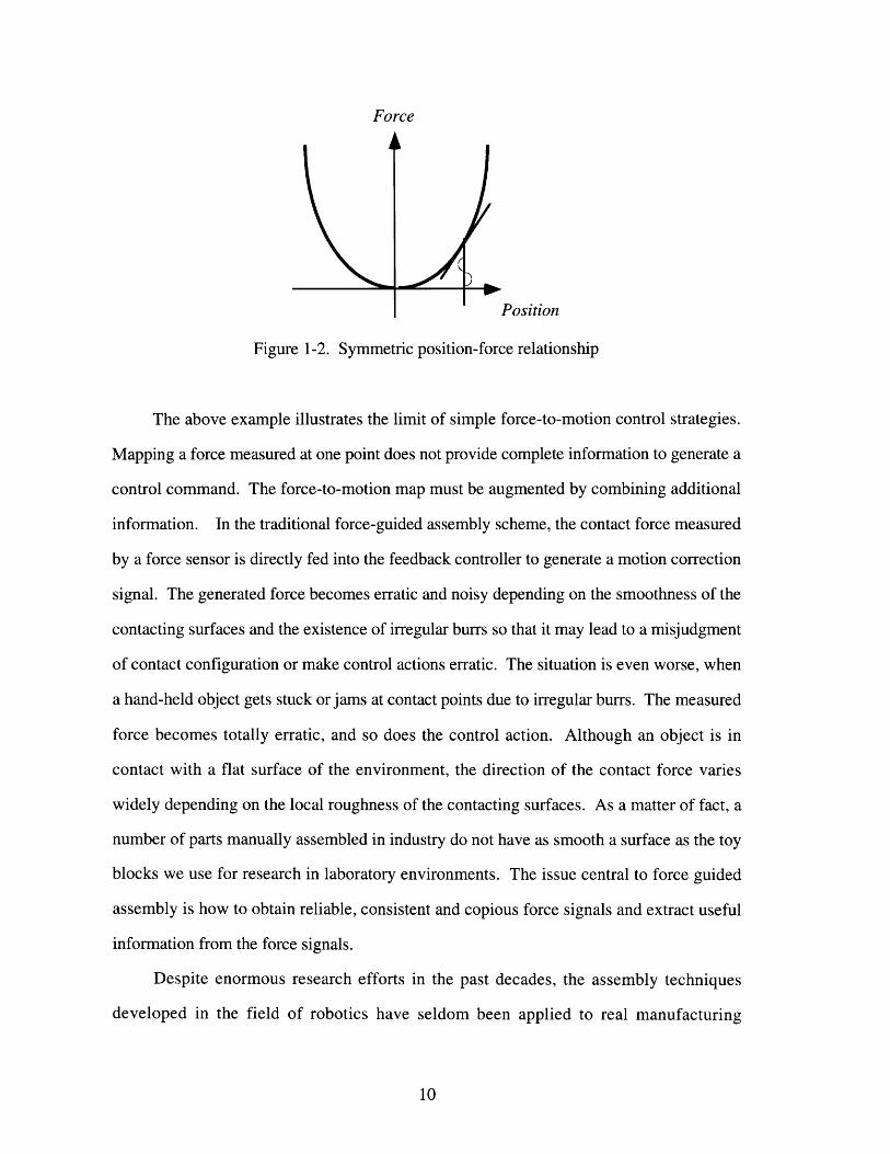
[McCarragher and Asada, 1994]. As shown in Figure 1-2, let us suppose that the goal is

to find the position where the reaction force is minimum and the robot should be directed

towards decreasing force. Since the force profile is symmetry, the robot cannot decide

which way to proceed to reach the goal. The force information obtained at one point does

not contain sufficient information to determine the direction of motion. Additional

information such as the gradient of the force profile is necessary for determining the

appropriate direction.

Force

A

Position

Figure 1-2. Symmetric position-force relationship

The above example illustrates the limit of simple force-to-motion control strategies.

Mapping a force measured at one point does not provide complete information to generate a

control command. The force-to-motion map must be augmented by combining additional

information. In the traditional force-guided assembly scheme, the contact force measured

by a force sensor is directly fed into the feedback controller to generate a motion correction

signal. The generated force becomes erratic and noisy depending on the smoothness of the

contacting surfaces and the existence of irregular burrs so that it may lead to a misjudgment

of contact configuration or make control actions erratic. The situation is even worse, when

a hand-held object gets stuck or jams at contact points due to irregular burrs. The measured

force becomes totally erratic, and so does the control action. Although an object is in

contact with a flat surface of the environment, the direction of the contact force varies

widely depending on the local roughness of the contacting surfaces. As a matter of fact, a

number of parts manually assembled in industry do not have as smooth a surface as the toy

blocks we use for research in laboratory environments. The issue central to force guided

assembly is how to obtain reliable, consistent and copious force signals and extract useful

information from the force signals.

Despite enormous research efforts in the past decades, the assembly techniques

developed in the field of robotics have seldom been applied to real manufacturing

processes. Sophisticated techniques such as admittance control [Whitney, 1977], stiffness

control [Salisbury, 1980], back projection [Lozano-Perez, Mason and Taylor, 1984]

[Erdmann, 1986] and contact recognition [Asada and Hirai, 1989] [Desai and Volz, 1989]

[Xiao, 1993] have been developed and tested successfully, but only in laboratory

environments. In manufacturing industries, most assembly tasks are performed either

manually or by simple machines. Products are designed so that their assembly can be

performed simply by standard machines. This so-called design for assembly has been the

major thrust in today's manufacturing technology. Simplification and standardization must

be pursed further, but it should be noted that complex, non-standard parts that cannot be

assembled by standard techniques are almost always involved in most products. Such

parts, although few in number, are currently very costly as they are assembled manually.

Difficult assembly tasks include: i) odd-shaped electronic parts such as connectors, heat

sinks, and shields of RF circuits, ii) plastic covers and structures of consumer electronics

and appliances, iii) sheet metal and composite parts of automobiles and aircraft, to name a

few. These parts are difficult to deal with, since they are highly complex, inaccurate and

sometimes deformable, having large tolerance errors. For example, sheet metal parts

produced by shearing and stamping are complex and deformable and, more importantly,

they have large, sharp burrs that often make assembly operations difficult. When burrs

exist, friction becomes highly unpredictable and erratic, preventing smooth mating

operations. The assembly operations required for these parts are complicated, yet the task

must be performed reliably to meet high quality requirements.

1.2 Objectives and Outline of the Thesis

In this thesis, a novel technique for overcoming the difficulties in the force-guided

assembly for real manufacturing applications will be presented. Instead of simply receiving

force information from the assembly process, we give perturbation to the robot end effector

and measure the reaction forces to the perturbation. By taking the correlation in between,

reliable information for guiding the endeffector will be extracted and used for control. The

dither, a small amplitude perturbation has been used in many practical ways, but the

proposed perturbation/correlation method is different from the previous ones in that the

dither is used for the purpose of estimating the gradient of a performance index as well as

for friction suppression and that a force feedback loop is formed around the assembly

process. Our goal is to guide an assembly part based on force information. Perturbation

commands are used as a means to build an effective force feedback loop rather than merely

suppressing friction in open loop control.

The technique using perturbation and correlation has been developed, and the

undecidable problem shown above was resolved . The end effector is perturbed with a

known frequency, in turn the reaction force in response to the perturbation is measured,

and its correlation with the perturbation input is computed. The resultant correlation

provides the gradient of the force profile, which allows the robot to decide which way to

proceed to reach the goal. To implement this method, various parameters including the

perturbation frequency and feedback gains must be tuned with care so that the overall

stability of the system may be maintained.

The basic concept of perturbation/correlation based control is described in chapter 2

with application to a force guided robot. In chapter 3, we applied this algorithm to a pipe

insertion task for a case study. The robot with the environment is modeled with

experimental data. A guideline to select several parameters involved in this controller is

shown based on the analysis and verified with simulation. In the chapter 4, based on the

model, stability analysis is conducted including the unknown nonlinear environment. A

vibratory end effector is designed and implemented and with this end effector, the

experiment is discussed in chapter 5. Other than the pipe insertion case study, this

perturbation/correlation based control is applied to the connector assembly task in chapter 6

followed by the conclusion.

Chapter 2

Control Architecture

2.1 Introduction

For a force-guided robot control, the perturbation/correlation based controller is

introduced. For most of the assembly tasks by robot, it is required to control the

displacement and force. Especially, when there exists uncertainties involved in the

assembly task, preprogrammed displacement and force trajectories don't work well. We

need to cope with these uncertainties to successfully accomplish the task. Still, the force

and displacement are very important information to guide the robot. Our approach is, first

set up a performance index which clearly represents the task, and then make a controller to

minimize this performance index based on perturbation/correlation. This performance

index as well as the control variables we perturb and update should be chosen very

carefully. In the following chapters, the basic idea of the perturbation/correlation algorithm

is described, and then applied to a force-guided robot system.

2.2 Perturbation/Correlation

The perturbation/correlation method is a direct control method which involves

perturbation, correlation and adjustment. For example, consider a plant with appropriate

inputs, having unknown environment, and a means of continuously measuring a

performance index. The inputs can be changed to affect this performance index. the

question is how to adjust this input to get the optimum performance index. The most direct

and simplest procedures would be to adjust the input and see the effect on the performance

index. However, in a practical problem, the number of parameters to be adjusted, the

presence of output noise, the parameters of the plant may vary with time and nonlinearities

may be present in a plant. The feasibility of this method would depend on the stability of

the overall system as the plant parameters varied with time. The role of the perturbation is

giving variations to the input. The correlation is to estimate the change of the performance

index with respect to the change of the input, in other words, the gradient of the

performance index. Based on this estimate of the gradient we can adjust the input so that

we can minimize the performance index. From now on, we will prove the correlation

corresponds to the gradient.

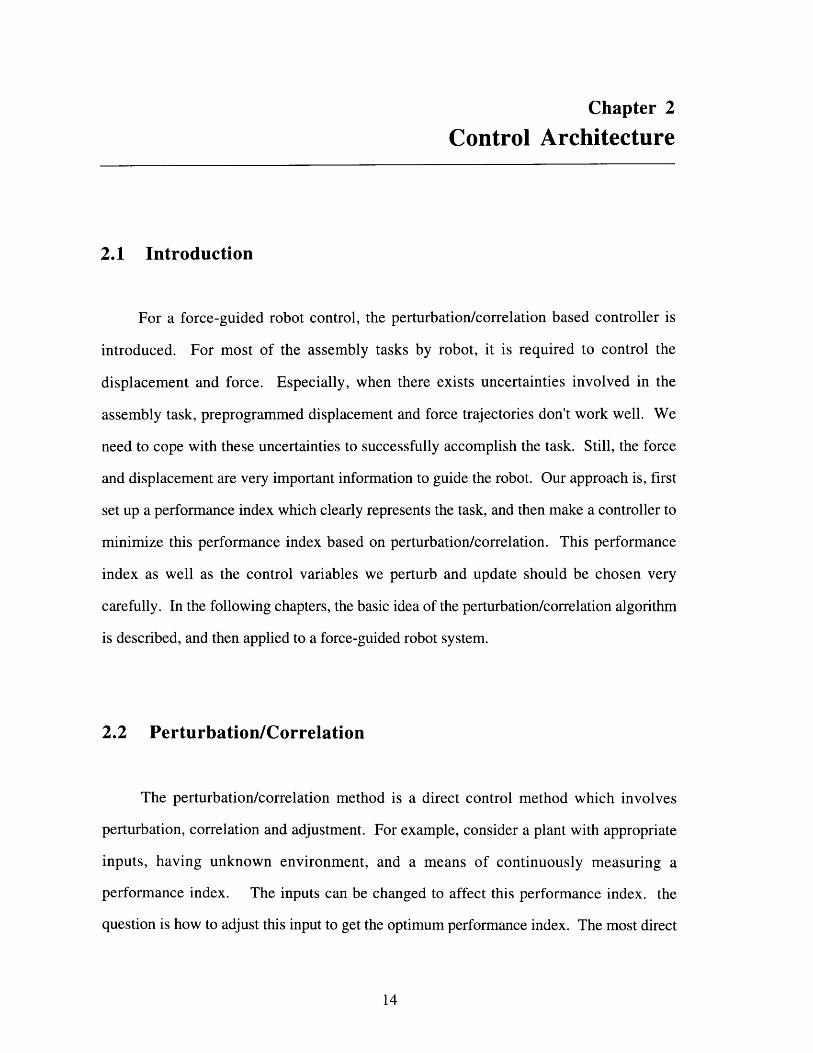
Consider a performance index, F, with input x as in Figure 2-1. Even though we

don't know the exact mathematical representation of F, by locally perturbing the input x,

we need to estimate d around a local region.

x F(x) - F

Figure 2-1. Performance index F and input x

Assuming that we can choose the value of x and observe the corresponding value of F at

every instant, the objective is to determine a procedure for adjusting x so that it converges

to the optimal value, Xoptimal which give the minimum value of F.

F(x)

A

-

)

I

I

X1 Xoptimal X2

Figure 2-2. Perturbation Method

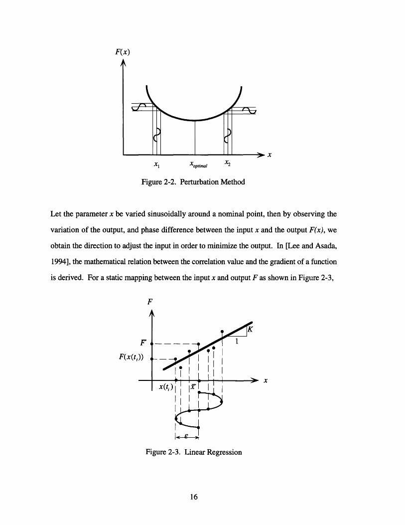
Let the parameter x be varied sinusoidally around a nominal point, then by observing the

variation of the output, and phase difference between the input x and the output F(x), we

obtain the direction to adjust the input in order to minimize the output. In [Lee and Asada,

1994], the mathematical relation between the correlation value and the gradient of a function

is derived. For a static mapping between the input x and output F as shown in Figure 2-3,

F

F(x(ti

x

Figure 2-3. Linear Regression

I

- r

O

let x be an input command to one of the robot control axes, which is varied sinusoidally

around its nominal value, xo so that

x(t) = xo + EA (t) (2-1)

3x(t) = sin(opt) (2-2)

where E and w, are, respectively, the amplitude and frequency of the sinusoidal

perturbation. Let F(x) be the performance index corresponding to the input. The

correlation between x and F(x) is given by

t+ -XRx = f' 3x()F(x(T))dz (2-3)

where the integral interval is over one complete period of the perturbation. When the force

is sampled at time t, = - i = 1,. ,2n, eq.(2-3) reduces to

2n

x = XF(ti)esin(- i) (2-4)i=1

From the linear regression, the slope at the point 1, is defined as

Ix(ti) - i][F(ti)- FK= i=12n (2-5)

[x(ti)- X]2

where,

2n

1 2nS= n F(t) (2-7)

Substituting eq.(2-1) into eq.(2-5) yields

2n 2n

EYsin(a-i)[F(ti) - F] ~F(ti)sin(~ i)K = i=1 (2-8)

Se2 sin 2(i) nEi=1

Comparing eq.(2-8) with eq.(2-4),

RP = nE2K (2-9)

Namely, the correlation given by eq.(2-4) represents the gradient of the function at the

nominal point multiplied by known constants. For the sake of simplicity, the above

formulation of correlation is only for one dimensional perturbation. This can be extended

to multi-input, multi-output correlations by using standard techniques [Eveleigh,1967].

The above example is based on a static mapping between position and force relationship.

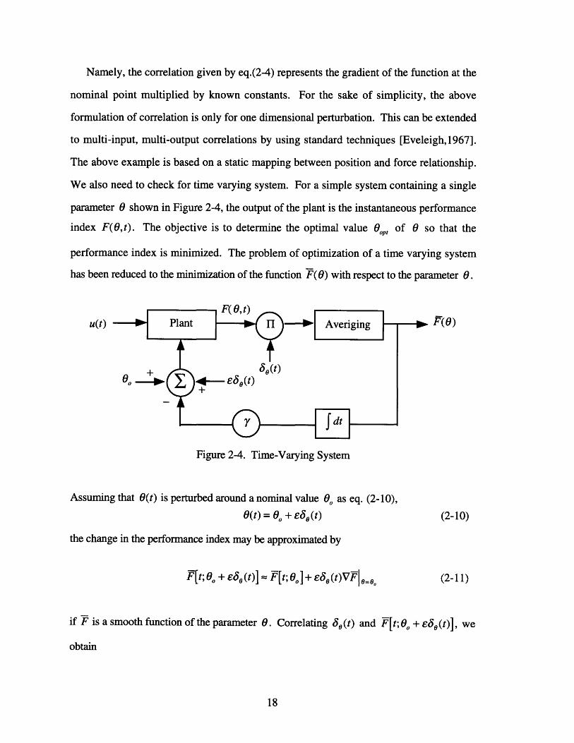
We also need to check for time varying system. For a simple system containing a single

parameter 0 shown in Figure 2-4, the output of the plant is the instantaneous performance

index F(O,t). The objective is to determine the optimal value Bop, of 0 so that the

performance index is minimized. The problem of optimization of a time varying system

has been reduced to the minimization of the function F(0) with respect to the parameter 0.

u(t) F(e)

Figure 2-4. Time-Varying System

Assuming that O(t) is perturbed around a nominal value 0o as eq. (2-10),

O(t) = 0o + E, (t) (2-10)

the change in the performance index may be approximated by

F[t; 0o + e3 (t)] = F[t; 0 o ]+ e3(t)VF o= 0o (2-11)

if F is a smooth function of the parameter 8. Correlating So(t) and F[t; o0 + e3o(t)], we

obtain

Se (t)F[t; 0(t)]= e (t)F[t; o] + E3 (t)VP7 lo=0 (2-12)

Assuming that So (t) is independent of the input u(t) and has an average value zero, the first

term can be neglected. The second term in eq. (2-12) yields a quantity which is

approximately proportional to the gradient of F with respect to 0 at the operating point o0.

This quantity is used for updating the parameter 0. A simple gradient descent method

allows this system to reach the optimal point. The parameters of interest are the amplitude

and frequency of the perturbation and the gain in the feedback loop. Selection of these

parameters are discussed in detail in chapter 3 with pipe insertion task, but briefly,

i) too small a value of the amplitude makes the determination of the gradient difficult

while too large a value may overlook the optimum value

ii) a very high frequency of perturbation may have negligible effect on the output while a

low value of it requires a long averaging time.

iii) a large step size of the which gain may result in hunting or even instability while a

small value of it would result in very slow convergence.

2.3 Application to the Force Guided Robot

Consider a robot system which has the internal position controller. The end effector

is interacting with an environment doing a task, such as peg-in hole, inserting a pipe or

palletizing a box. As the robot moves, in other words, as the displacement of the end

effector changes, the force response from the environment would be changed, too. If we

could set up a performance index, which clearly represents the task, then by minimizing the

performance index, we can successfully finish the task. The question is how we can

minimize the performance index. The information we could get is the reaction force, and

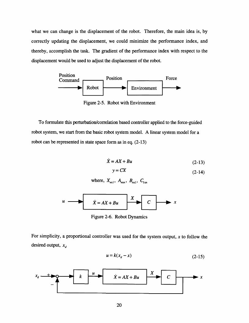
what we can change is the displacement of the robot. Therefore, the main idea is, by

correctly updating the displacement, we could minimize the performance index, and

thereby, accomplish the task. The gradient of the performance index with respect to the

displacement would be used to adjust the displacement of the robot.

PositionCommand Position Force

SRobot - Environment -

Figure 2-5. Robot with Environment

To formulate this perturbation/correlation based controller applied to the force-guided

robot system, we start from the basic robot system model. A linear system model for a

robot can be represented in state space form as in eq. (2-13)

= AX + Bu (2-13)

y = CX (2-14)

where, Xnx , Anxn , Bnxl, Cx n

u X = AX + Bu - 1 C - x

Figure 2-6. Robot Dynamics

For simplicity, a proportional controller was used for the system output, x to follow the

desired output, xd

u = k(xd - X) (2-15)

Xd x

Figure 2-7. Robot with Position Controller

The original system equation with proportional controller can be represented as in Figure 2-

8.

X = (A- kBC)X + kBxd

Figure 2-8. Simplified Representation

We have a performance index dQ(x), which is a function of x.

Figure 2-9. Performance Index

and we want to minimize performance index 4(x), by changing The

correlation/perturbation part gives the gradient of 1(x) with respect to x, that is, 0x.

D(x)

Figure 2-10. Perturbation/Correlation

For this perturbation/correlation part to be represented as a block diagram of which the

input is x, and output is "'x) shown in Figure 2-11, the following condition should be

satisfied.

IXd --

X C ----- No. X

x ---- - 77- -- '-• --

Figure 2-11. Gradient of the Performance Index

A performance index D is a function of the input x, and several other variables, z ,' ", z .Z

( = I(x,z1, z9,,, ZmZnm+ ... Z,) (2-16)

To get -, we perturb the input x as in eq. (2-17)dX )W·Y·LLVLI~IIU 111CY LlI

x(t) = x o + 3x(t) (2-17)

Let's assume that some of the other variables also have perturbations. For i = 1-. m

z,(t) = Zo,i + z,i(t) (2-18)

and for i = (m + 1)... n

zi(t) = Zo, i (2-19)

Assuming that ( is differentiable with respect to Y and zl , - , z , ( D is expanded as :

[X(T + At),Zl ( + At),- ,Zn (t + At)]

= D[x(),Z(), z ... , z, ()]+ Sx (t) 4x x + S dzIdzn

z c Z",+ 0(2)(2-20)

ignoring the higher order term, O(2), and because Sz,i(t) is zero for i = (m + 1).. --n, eq.

(2-20) becomes

44[X(T),Z r),. ( ",Zn (T)] + 5X x(t) dx + Ozl(t)d +* .. +45Z t) d(d T i ' r 'z dTm (2-21)

Correlating D and Jx, and taking average for one period of perturbation: [0, ], we

obtain

Y, JD 4R x(r), z(,) Z... , z (r)]3 (t)dt +

( _x (tt zl )-2- d t f . _ dtI,(,) dt + J 2 / o3(t) 1(t) - dt+...- J2Y X (t)3z, (d

Y./ 9X T W dz1 T ,19 '

(2-22)

We are perturbing 6x (t) sinusoidally as in eq. (2-23)

Sx (t) = esin wt (2-23)

therefore, eq. (2-22) becomes

6,= 2 d~- 1 +·dxxd' r2Y X (t) 6 1 (t)dt + ' ' m l_ x(t)zm(t)dtd T dz TM r 2

(2-24)

The first term in eq. (2-24) vanishes and the second term provides the gradient

multiplied by a known constant e2yr.

negligibly small. If we check eq. (2-25)

The remaining terms should be zero or made

-2%2 x ,) (t) zi(t)dt

this term becomes zero when x (t) and 3z,i(t) are orthogonal, for example,

Sz,i(t) = Ei cos Wt

then,

2 Jx (t)ozi(t)dt = 0_2 )/

(2-25)

(2-26)

(2-27)

In case the variable 8,,2 changes linearly with respect to time as in eq. (2-28)

6z,i(t) = Eit (2-28)

then, eq. (2-25) becomes

. x(t) z,i(t)dt= (2-29)T_2% o92 (2-29

Since it is inversely proportional to w 2 and proportional to Ei, we can make this term

negligibly small by increasing the perturbation frequency o with small e,. Based on this

gradient value -p-, we update x so that we can decrease performance index as in eq. (2-

30).t0 tO(x)Xd = o- j-x dT (2-30)

For this perturbation/correlation control, a feedback loop was implemented to update the

desired output in order to minimize the performance index Q((x).

Xo X

Figure 2-12. Robot System with Perturbation/Correlation

We showed in the previous section that the correlation/perturbation algorithm gives the

gradient value of the performance index. By introducing an extra variable, x,, the

augmented system can be represented as in eq. (2-32) and eq. (2-34)

Xa = Xd (2-31)

xa= - x (2-32)

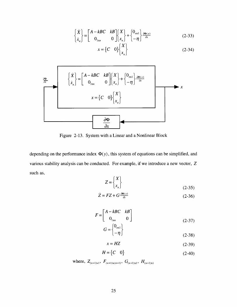
F =[A-kBC kB] X+ n0 6(x)=a+ IL l i dx

xa OIxn 0 JXa -

x={C O}X Xa

IX [A - kBC kB t X t Ont dx

xxa O{xn 0 xa -

x={C 01}(XXa

dxV~l,L dJ I

(2-33)

(2-34)

-~ x

Figure 2-13. System with a Linear and a Nonlinear Block

depending on the performance index 1(y), this system of equations can be simplified, and

various stability analysis can be conducted. For example, if we introduce a new vector, Z

such as,

Z=x -

I~aj (2-35)

Z = FZ + G _((y) (2-36)

F=[ A-kBC kB]

G = -O

x=HZ

H={C 0}where, Z(,+l)Xl, F(n+.ox(,n+l, G(n+l)xl, H(n+l)x 1

(2-37)

(2-38)

(2-39)

(2-40)

I

Based on this final system model, we can apply stability criterion. With the separated

linear part, and nonlinear part, this model is useful for applying nonlinear stability theory.

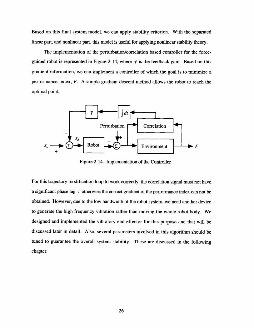
The implementation of the perturbation/correlation based controller for the force-

guided robot is represented in Figure 2-14, where y is the feedback gain. Based on this

gradient information, we can implement a controller of which the goal is to minimize a

performance index, F. A simple gradient descent method allows the robot to reach the

optimal point.

Fxo -+

Figure 2-14. Implementation of the Controller

For this trajectory modification loop to work correctly, the correlation signal must not have

a significant phase lag : otherwise the correct gradient of the performance index can not be

obtained. However, due to the low bandwidth of the robot system, we need another device

to generate the high frequency vibration rather than moving the whole robot body. We

designed and implemented the vibratory end effector for this purpose and that will be

discussed later in detail. Also, several parameters involved in this algorithm should be

tuned to guarantee the overall system stability. These are discussed in the following

chapter.

Chapter 3

Case Study : Pipe Insertion Task

3.1 Introduction

We formulated the correlation/perturbation based controller for a force-guided robot

in the previous chapter. For a case study, we applied this control algorithm for a robot

which inserts a pipe into a heat exchanger. As the robot inserts a copper pipe into the hole

of the heat exchanger, the pipe interacts with the layers of metal foils. First, we selected

the resistant force as a performance index for this task. By adjusting the position of the

robot end effector, we can reduce the performance index and successfully insert the pipe.

The characteristic of the force response is very nonlinear and simple 'force to position' map

is not working very well for this task. We modeled this robot and environment based on

the analytic model and experimental data. Also the guideline to select several parameters

involved in this algorithm is discussed with simulation result.

3.2 Pipe Insertion Task

The perturbation/correlation based control is applied to a practical assembly task,

*which is difficult to perform by traditional methods. Figure 3-1 shows the assembly of a

heat exchanger for an air conditioning system.

Copper Pipe 4Layer of -

Metal Foils

ZFigure 3-1. Pipe insertion task

The task is to insert a long copper pipe into a stack of thin sheet metals. The holes on the

sheet metal have a minimum clearance, in order to maximize the heat transfer efficiency.

Unlike the conventional peg insertion problem which deals with machined parts with clear

edges and surfaces, the surface of the hole created by the stack of aluminum foils is totally

irregular and rugged. Since the aluminum foils are made by stamping, the hole has

irregular burrs and poor tolerance error. As a result, the accuracy in fixturing the foils

become significantly low, and the wall of the holes created by the stack of the foils is

irregular as shown in the figure. In real plant production lines, this kind of pipe insertion

task has been performed only by human workers. Skilled workers insert pipes by

perturbing the pipes in order to avoid jamming as well as to determine which way to correct

the motion. According to them, the skilled workers monitor obstructing forces in response

to the applied perturbation, and modify their motion accordingly. Their skill is very similar

to our force sensing method described in the previous chapter.

The key information used in the pipe insertion is the reaction force in the pipe's

longitudinal direction, that is, the Z axis in Figure 3-1. This obstructing force, Fz, varies

in accordance with the perturbation of the pipe in the transversal direction, that is , the x

axis in the figure. The correlation in between is given by

R,(t)=fJ F (r)esin(or)dr (3-1)

The obstructing force is created at the contacts of the pipe against the wall of the holes. As

the pipe trajectory deviates from the center line of the hole, the obstructing force generally

increases, because the pipe's contact pressure against the wall of the hole increases. A

smaller obstructing force implies that the pipe's position is closer to the actual centerline,

where the pipe can be inserted smoothly. Therefore, we can use the obstructing force as an

index representing the deviation of the pipe's trajectory for the purpose of guiding the pipe

in the desirable direction. Figure 3-2 shows an approximate plot of Fz against

displacement x. The minimum point in the figure shows the plausible centerline position to

which the pipe's trajectory is to be corrected during the insertion.

Fz

x

Figure 3-2. Obstructing force Fz v.s. displacement x

In order to guide the pipe towards the minimum point of force Fz , we need to know

the gradient of the curve or its equivalent information. Note that the force measured at a

single point does not provide sufficient information as to which way the robot should

move. This is an undecidable situation. The correlation Rx(t) given by eq.(3-1) resolves

this problem since it directly provides the gradient information, as analyzed in the previous

section. Therefore, the control law to correct the trajectory of the pipe is simply given by

• |

~C~ontnr- &~qgCI

dt

where xd is the trajectory command to the x axis servo, and 7, the proportional constant.

Figure 3-3 shows the block diagram of the x axis control system, in which the nominal

trajectory xo is corrected based on the correlation Rx in accordance with eq.(3-2).

FzXo+

Figure 3-3. Robot with Perturbation/Correlation

This control system can be regarded as a type of direct adaptive control [Narendra

and Annaswamy, 1989], since the control system is driven towards the minimum point of

performance index Fz , directly by perturbing the control command xo. It should be noted

that the force measured is by no means a clear signal. The actual plot of Fz , against x is an

erratic, noisy one, unlike the conceptual plot in Figure 3-2. Nevertheless, the system can

behave smoothly because the correlation operation requires integral operations rather than

derivatives. To obtain the gradient information, we usually need derivative operations, but

this correlation method does not need derivatives but integrals, which are much smoother

and computationally more stable. For perturbation, we generate vibration using vibratory

end effector, so that we can not only generate high frequency dither, but also the whole

robot arm doesn't have to shake the whole arm. Also, we can separate the perturbation part

with robot controller, so that it makes easier to apply the stability theorem.

3.3 Modeling of the Process

In this pipe insertion task, the robot end effector is perturbed in the x direction and the x

coordinate of its trajectory is corrected while moving in the z direction at a constant speed.

The x coordinate is updated based on the insertion force Fz, in such a way that the x

coordinate is moved towards the minimum point of F,. Insertion force Fz is a function

not only of the x coordinate but also of the depth of insertion z and the insertion speed i.

As the depth of insertion increases, more aluminum foils may contact with the pipe and

generate a larger resistive force when the pipe is pushed into the hole. Therefore, as z

increases, Fz increases in general. Also, the resistive force varies depending on the

insertion velocity i. Hence, Fz is expressed as

Fz = 4(x,z,i) (3-3)

Function QD is an unknown function, but can be assumed that it has a minimum point with

respect to x.

z : depth ofinsertion

x

Figure 3-4 Insertion force varies depending on x, z and z

As shown in Figure 3-4, although the profile of function (D varies depending on z and j,

it is assumed that the function has a minimum with respect to x in each stage of insertion as

long as the insertion speed is constant. This assumption is supported by experimental data,

as will be discussed later.

We assumed F, is a function of x and z coordinates and also the velocity i. Also, it

has a minimum point with respect to x. To verify this assumption, we collected

experimental data with many different conditions as in Figure 3-5.

HeatCopper /Exchanger

Force sensor Pipe

LinearSlide -

Figure 3-5. Experimental Setup

Note that the displacement in the x-direction is fixed until it reaches the desired depth,

and the velocity in the z-direction is kept constant for each run. First of all, the resistant

force Fz is measured with slightly different x coordinates so that we could check that it has

a minimum point. We plotted the minimum resistant force profile with two nearby ones.

This experiment was repeated with several different velocity i. One of them is shown in

Figure 3-5 and we obtained similar results with different velocities.

Vz=15 [mm/sec]

30

251

20,

15,

LL 10,

5.

-5,4040

20

0 -0.5 0.5 1 1.5

Z [mm]X [mm]

Figure 3-6. Fz as a function of x and z

Figure 3-6 clearly shows that Fz has a minimum point with respect to x. Figure 3-7

shows F, with different velocity i. From this figure, F, is also a function of j, but it

doesn't highly depend on i. From these result, we verified that the Fz satisfies our

assumption.

NL1

Z [mm]

Figure 3-7. F, as a function of z and i

0

From these result, we verified that the Fz satisfies our assumption.

Based on the experimental verification, we can model the system without including the

movement in z-direction as second order system with mass m, damper b and spring Ke due

to the environmental stiffness. The displacement of the robot is represented as xr.

Xr

F

z

Figure 3-8. System modeling

mi, = -bx, - Kexr + F (3-4)

Control force is generated using a proportional controller.

F= K,( - Xr) (3-5)

The trajectory command, xd is generated based on the algorithm shown in Figure 3-9. It is

represented in eq. (3-6).

Figure 3-9. Block diagram representation

t AFxd= - y 7 -dz'r (3-6)

tO AkXr

where, yis a positive update constant and the initial nominal trajectory xo is usually zero.

To represent this system in a state space form, let

xI = x r (3-7)

x 3 = f z (3-8)

Then, the system equation is,

.1 = x 2 (3-9)

K, + Kp b K2 x1 2 3 (3-10)m m m

OdFx3 = (3-11)

d 1

3.4 Selection of Parameters

In this perturbation/correlation based control, there are several variables we should

select. For perturbation itself, we need to choose the values of amplitude and frequency of

the perturbation. For the feedback controller, we need to tune the feedback gain. This gain

is related to the stability of the system, and is discussed in the next chapter. The amplitude

of the perturbation is constrained by the geometry of the hole and the pipe. Especially, for

this heat exchanger, small clearance should be kept for heat conductivity. Therefore, we'd

better use small amplitude for perturbation. However, if we use too small amplitude, we

can't get meaningful force response but only the noisy signal. For the frequency, we can

guess that the higher is better, to get faster update. In this section, we do analysis to see

the effects of these variables.

Since the function QD is unknown, we perturb the end effector in order to obtain the

gradient -2F as mentioned in the previous section.

x(t) = xo + x (t)

x(t) = esin wt

(3-12)

(3-13)

The insertion speed is kept constant with a high gain position control in the z axis :

z(t) = zo + Vot (3-14)

Consider the insertion force Fz at time t = 7 + At. Assuming that Fz is differentiable with

respect to x and z, Fz is expanded as:

Fz[x( + At),z(r+ At), V] = Fz[x(r),z(,r), Vo]+ 3x (t) - zz=z(r)

+ Sz(t) )Fzdz x=x(r)

(3-15)where 8, = VoAt and 6(2) is a higher order small quantity. Correlating Fz and 6x, and

taking average for one period of perturbation : [0, -], we obtain

F, y FZ [x( ), z ( r), V0 ] (t)dt + T8x (t)2 d~zOi23 2Y dx x=x(,r)

z=z(-r)

E2 dF 27rExoF = 0 + - 2 Vo0 dx x=x(r) 02

Z=Z(T)

PTF

JIr-2/ .dz lx=x(r)z=z( r)

(3-16)

_ [(3-17)dz x=x(r)zZ z=Xr)

The first term in the above equation vanishes when integrated over one perturbation, anddF.the second term provides the gradient --- multiplied by a known constant e2K. The third

term can be interpreted as an offset due to the motion in the z direction. The offset,

however, can be made negligibly small by increasing the perturbation frequency w and

decreasing the insertion speed, since it is inversely proportional to c 2 and proportional todFVo . In order to correctly estimate the gradient -g- from correlation 3xFz, this offset must

+ t(2)

dt + VtI ,(t)_- l

be negligibly small. The perturbation frequency c and the insertion speed must be

determined so as to meet this requirement.

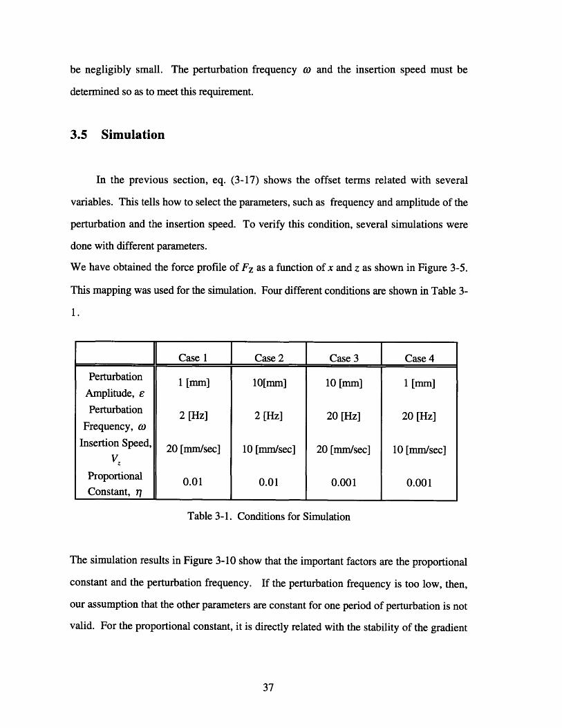
3.5 Simulation

In the previous section, eq. (3-17) shows the offset terms related with several

variables. This tells how to select the parameters, such as frequency and amplitude of the

perturbation and the insertion speed. To verify this condition, several simulations were

done with different parameters.

We have obtained the force profile of Fz as a function of x and z as shown in Figure 3-5.

This mapping was used for the simulation. Four different conditions are shown in Table 3-

1.

Case 1 Case 2 Case 3 Case 4

Perturbation P1 [mm] 10[mm] 10 [mm] 1 [mm]Amplitude, e

Perturbation 2 [Hz] 2 [Hz] 20 [Hz] 20 [Hz]Frequency, (o

Insertion Speed, 20 [mm/sec] 10 [mm/sec] 20 [mm/sec] 10 [mm/sec]V

Proportional 0.01 0.01 0.001 0.001Constant, 7

Table 3-1. Conditions for Simulation

The simulation results in Figure 3-10 show that the important factors are the proportional

constant and the perturbation frequency. If the perturbation frequency is too low, then,

our assumption that the other parameters are constant for one period of perturbation is not

valid. For the proportional constant, it is directly related with the stability of the gradient

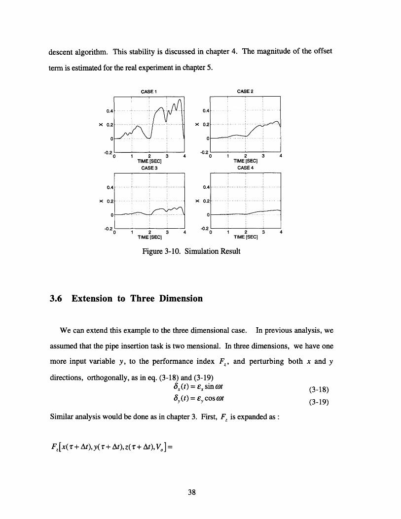
descent algorithm. This stability is discussed in chapter 4. The magnitude of the offset

term is estimated for the real experiment in chapter 5.

CASE1 CASE2

0.4..

x 0.2

0

X

0 1 2 3 4TIME [SEC] TIME [SEC]

CASE3 CASE4

0.4

X 0.2

0

0.4

x 0.2

0- 3

0 1 2 3 4 0 1 2 3 4TIME [SEC] TIME [SEC]

Figure 3-10. Simulation Result

3.6 Extension to Three Dimension

We can extend this example to the three dimensional case. In previous analysis, we

assumed that the pipe insertion task is two mensional. In three dimensions, we have one

more input variable y, to the performance index FZ , and perturbing both x and y

directions, orthogonally, as in eq. (3-18) and (3-19)5x(t) = Ex sin (ot (3-18)•,(t)= e,cos (t (3-19)

Similar analysis would be done as in chapter 3. First, Fz is expanded as :

F, [x( + At), y( r + At), z(Tr + At), V] =

4

.........................................

+ y ,(t)•-Fz=z(T)

z+ (t) z x- xr)dz -y(2r)

z=z(r)

(3-20)

Correlating Fz and 8x , and taking average for one period of perturbation: [0, ], we

obtain

SxF, 2Y Fz 8x (t)dt +

+ 2% Votx (t)ýF dtJT--2n/o z ,I.Fz S (t)2 dt + 6 (t)2 ,(t)tdt

with eq. (3-18) and (3-19), eq. (3-21) becomes

3SF 2 CE xSx F = Exx,-- 2 xco Vox dx W 02-iz,dFzz T

(3-21)

(3-22)

and also correlating Fz and 8,,, and taking average, we obtain

V6,7 2 Fz 2 ý , (t)dt +ax<

t)(t)dt + F z (t)2 dt Vot(tdF, I

(t Idz (3-23)

Again, with eq. (3-18) and (3-19), eq. (3-23) becomes

43vFz= E2,rdJ

(3-24)

Note that we the offset term only in eq. (3-22). Table 3-2. shows the comparison between

the 2D and the 3D analysis.

Fz[X(T), y(T),'z(T), Vo] + 8x(t)- x )dx =rz=z(r)

Coordinate

Performance

Index

Perturbation

V

Control Law

X

z

Fz = F (x,z, i)

3x(t) = esin wot

VoXd = Xo -nJ4~ dr

Y xz

Fz = Fz(x,y,z,i)

3x(t) = ex sin cot

•,(t) = e, cos ot

Voxd = Xo - flJo dr

Yd = Yo - -1-d dr

Table. 3-2

Simulation was done for this case. Figure 3-11 shows the trajectory time history, and

Figure 3-12 shows the performance index, F,.

2D 3D

-10

-20

NN-30

-0.50.5

L ...... J EX immj

Figure 3-11. End Effector Trajectory

0.8,0.8~ initial

0.6,

L0.4-

0.2

0 (

0.5 final

0 0.50

-0.5 -0.5

Y [mm] -1 -1mm]

Figure 3-12. Performance Index Time History

We have shown that this controller can be used for three dimensional case by simulation.

41

-40

r_ I

::: :-::

-..

Chapter 4

Stability Analysis

4.1 Introduction

In the previous chapter, we have developed a model of the pipe insertion task. Based

on this model, we need to check the stability of the whole system. We get a linear system

model including the perturbation/correlation part, however, we still don't have exact model

of the performance index, which is Fz. This is actually unknown and can not be

represented exactly by mathematical expression. We assumed that it has a parabolic form,

and has a minimum point. From the experimental data, we verified that our assumption is

correct, but still its exact shape is not known, which depends on the holes and many other

characteristics. We start from a simple parabolic form of Fz so that the whole system

becomes linear. In the following section, we get the stability boundary by applying Popov

theorem even though the performance index is not known and nonlinear.

4.2. Linear System

Based on system model in the previous section, we check the stability of the system

based on Routh's stability criterion. Consider the perturbation/correlation based system

shown in Figure 4-1.

Figure 4-1. Block diagram representation

For simplicity, let's assume the Fz is a parabolic function as in eq. (4-1)

1Fz = -1axl2 +c

2(4-1)

where, a > 0

we have the transfer function of the system as in eq. (4-2)

(4-2)i(s) =ms2 +bs +Ke

and the trajectory command is updated based on eq. (4-3)

Xd = Xo - Y o-- Ar

(4-3)

where, yis a positive update constant and the initial nominal trajectory xo is usually zero.

To represent this system in a state space form, let

X1 = X2

K+p bK, + K, bxi2 x1 -- X 2m m

dF3 x Z

K

m

(4-4)

(4-5)

(4-6)

,,

with eq. (4-1), eq. (4-6) becomes

x3 = ax1 (4-7)

The system's state equations are given by,

J2i3,

1/11 0 x,

-bP x2 (4-8)m mO 0 _ X3

and the characteristic equation is,

ms 3 + bs2 + (Kp + K,)s+ yaKp = 0 (4-9)

From Routh's stability criterion, we get stability condition as in eq. (4-10)

b(K, +K,)0 < y < (4-10)amKp

4.3 Nonlinear and Unknown System

The stability analysis in the previous section was done using Routh's stability criterion,

but that was based on the assumption that the nonlinearity has a parabolic form, so that we

can transform the system into a linear one. However, in the real assembly task, this

displacement-to-force map is not well known. To be more practical, we need to find out

the conditions of the stability not only for the parameter values in the controller, but also the

characteristics of the nonlinearity. We are applying Povpov criterion for this purpose.

In the system considered in Figure 4-2, the forward path is a linear time-invariant

system, and the feedback part is a nonlinear static mapping.

Figure 4-2. System with nonlinearity

The equation of this system can be represented as,

= AX - BDQ(y) (4-11)

y = CX (4-12)

G(s) = C[sI- A]-' B (4-13)

where, D is a nonlinear function. To check the stability of this system, Popov criterion

imposes several conditions for asymptotic stability.

Conditions

* A has all the eigenvalues with non positive real parts but with only a simple zero

eigenvalue.

* (A,B) is controllable

* (A, C) is observable

* Nonlinearity Q belongs to a sector [0,K]

* there exists a strictly positive number a, such that1

Vcoý 0, Re[(l + jaw)G(jo)] + - > E (4-14)K

for an arbitrarily small e > 0, then, the point 0 is globally asymptotically stable.

let G(jw) = G,1 (jwo) + jG2 (jco), then,

G,(jo) - awG 2(jo)+ 1 + E (4-15)K

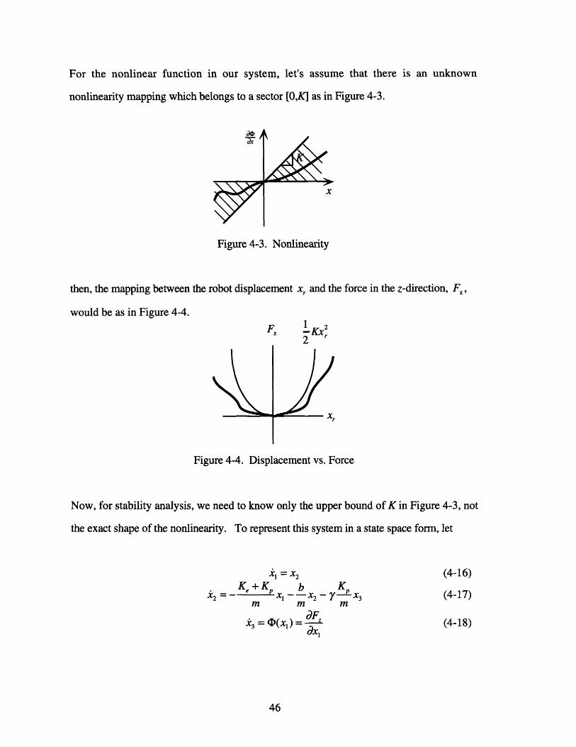
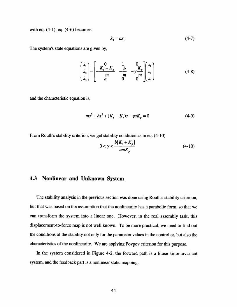
For the nonlinear function in our system, let's assume that there is an unknown

nonlinearity mapping which belongs to a sector [0,K] as in Figure 4-3.

dx

x

Figure 4-3. Nonlinearity

then, the mapping between the robot displacement x, and the force in the z-direction, Fz,

would be as in Figure 4-4.

Fz 1-Kx22

Xr

Figure 4-4. Displacement vs. Force

Now, for stability analysis, we need to know only the upper bound of K in Figure 4-3, not

the exact shape of the nonlinearity. To represent this system in a state space form, let

x' = x 2 (4-16)Ke + Kp b KX

x2 2 (4-17)m m m

C3 (xl) •• (4-18)dxI

L

0 1A= K, + Kp b

m m0 0

B= 0]

-1l

C=[1 0 0]

and check the condition of Popov stability,

* eigenvalues of A { -b b2 -4m(Ke+K )2m

* (A,B) is controllable

* (A,C) is observable

Now for graphical interpretation, the system transfer function of the linear part is,

G(s) =

G(jo) =

G(jco) =

ms 3 + bs2 + (K, + Kp)s

,yKp

-b 2 + j[-m3 + (K, + Kp)o]

-byKw 2 + j[mw3 - (K, + Kp )o]b'w4 3 +[-m3 +(K, + K,)•2]

0KP-Y

m

0

(4-22)

(4-23)

(4-24)

(4-19)

(4-20)

(4-21)

the real part of G( jw) is

Re[G(jo)] =

and the imaginary part of G(jw) is

Im[G(jw)] =

-byKo 2

b2 o 4 +[ 3 + (K, + Kp)(] 2

mO) 3 - (K, + Kp)(

b 2oW4 +[-mwo3 + (K + Kp ) ]2

let's define

Im[G*(jco)] = o Im[G(jw)]

then,mm 4 - (K e + Kp)O 2

Im[G*(jw)]= 4 (Ke +b2W4 +[-mO +(K, +K, )w]

to plot eq. (4-25) and eq. (4-28) on Re[G(jw)] and Im[G*(jm)] plane,

several points. First of all, for co = 0

Re[G(jo))]= - b 2Kp

(Ke + Kp) 2

for co = oo

' 1Im[O (o)]- K

Re[G(ja)]= 0

Im[G*(j()]= 0

for Im[G*(jm)]= 0

for co = oo

we need to check

(4-29)

(4-30)

(4-31)

(4-32)

f Ke + Kpm

(4-33)

Re[G(jwo)]= - y Kb(K, +K,)

and finally to get the slope,

dlm[G*(jo)] -

3 Re[G(jco)]dIm[G*(j)] dao

dw dRe[G(jw)]

d Im[ G* (jm)]•

d Re[ G(jm)]

(4-25)

(4-26)

(4-27)

(4-28)

(4-34)

(4-35)

dIm[G*(jw)] (K + K,)b2 -(Ke + K+)2 m + 2(Ke + KP)m 2w 2 - m3) 4

dRe[G(jw)] bKy[b2 -2(K, +K,)m+2m2w2]

(4-36)

the slope for w = 0

Im[G*(0)] = (Ke + Kp)[b2 - (K + KP)m]dRe[G(O)] bKpy[b2 - 2(K, + Kp)m]

and for co = wo

dIm[G*(j.o)]_ (K, + K,)

dRe[G(jco)] ybKp

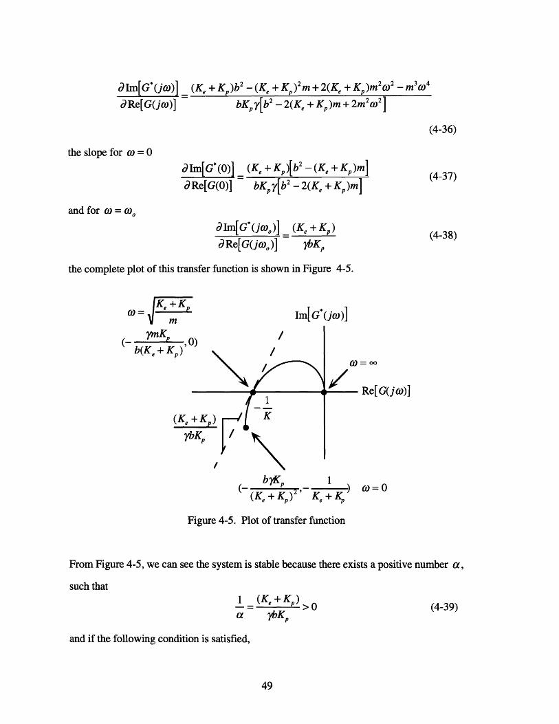
the complete plot of this transfer function is shown in Figure 4-5.

(4-37)

(4-38)

FKe + -K1) mm

b(nK +

b(Ke + Kp)'

Im[ G*(jw)]

/

/

/

(Ke74

/

b K•p 1

(K, + KP) K, +K

Figure 4-5. Plot of transfer function

From Figure 4-5, we can see the system is stable because there exists a positive number a,

such that1 (K,+ Kp)- = >a ybK,

(4-39)

and if the following condition is satisfied,

Re[G(jo)]

w=O0

1 ymK,- 1 < nKp (4-40)

K b(K, + K,)

Therefore, the system is stable when,

b(K, +K)Y < (4-41)

mKK

Comparing eq. (4-41) with eq. (4-10) in the linear case, both are the same, but this Popov

criterion is based on sector nonlinearity, of which the shape of the nonlinearity is not

known exactly. Therefore, once we get the maximum value of slope in the sector, we can

get the stability condition even though there exists an unknown nonlinearity.

4.4 Simulation

To verify the stability condition of eq. (4-10), let us choose the following parameter

values based on the estimation of the real system.

m = 0.042 [Kg]

b = 2.1 [Nsec/m]

Ke = 133 [N/m]

Kp = 100

and for simplicity, let's assume the nonlinearity is a parabolic form of

a = 0.5

then, the maximum value of the proportional constant in the update law is,

b(K, + K )'Yx = amK = 58.25

amK,

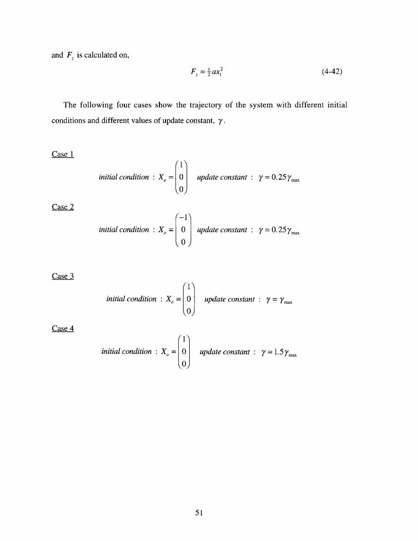
and F, is calculated on,

Fz = _ax (4-42)

The following four cases show the trajectory of the system with different initial

conditions and different values of update constant, y.

Case 1

initial condition : Xo

0'1

0

Case 2

initial condition : Xo

update constant

update constant

y = 0.25Ymax

y = 0. 25~max

Case 3

initial condition : X = 0i

initialinitial condition : X0 = 0

SOJ

update constant : Y = 7max

update constant :

Case 4

y = 1.5 7max

r=0.25*r_max4....

-2

-4

-6-1 0 1

x

r=r max20

10 ........... ... ....... .. in al

0 ........ ......

-1 0 ......... .. ........ .... .. ... .. .

-20-2 0 2

r=0.25*r_max6

4 ..... ·... . :.

4 t ·- ·- · ·- ..............i- -.. .... .....

2 " ................... " : "" 'i: -..i ....... ? ": .......

" 0 . ....... .* .

-4-1 0 1

xr=2*r_max

5000

S........

-500-500 0 500

x

Figure 4-6. Simulation Results for Linear Case

Figure 4-6 verifies the stability analysis in section 4.2. For case 1 and case 2, the system is

stable regardless of the initial condition. For case 3, the system is marginally stable with

maximum value of update constant. The system diverges with larger value than the

maximum update constant in case 4.

In order to verify the condition for the nonlinear case, a random force function which

belongs to the sector [0,1] is generated as shown in Figure 4-7.

01

8

6

4

2

0

-2

-4

-6

-8

-10SIi

Figure 4-7. Nonlinear Force Function

Similar simulations were performed based on this nonlinear force function. The result is

shown in Figure 4-8.r=0.25*r_max r=0.25*r_max

U.0

0

-0.5

_1

0.50

0

-1 -0.5 0 0.5 1 -1 -0.5 0 0.5 1x x

r=r.max r=1.5*rmax

0

X,

-1 0 1 -4 -2 0 2 4x x

Figure 4-8. Simulation Results for Nonlinear Case

The Popov stability criterion is more conservative than the linear case, so even with the

maximum value of the gain, the system converges. Therefore, once we found a sector the

nonlinear function belongs to, we can calculate the maximum stable gain. With the real

experimental data obtained in chapter 3., we have the sector value of the nonlinearity in our

system. One conservative estimate is,

K = 2x10 7 [N/mm 2

and then, the maximum proportional feedback gain is,

ymx = 5.825x10-6

Therefore, we selected a feedback gain less than this maximum value for the experiment.

53

.. ......... .... . .... .............

.. ......... ...... ............... ....

.. ... ................. ..... .........

.. .... . . .. ....... ........

I x x4 ·

_•[· ·,,=,o I

Chapter 5

Experiment and Implementation

5.1 Introduction

We have generalized the perturbation/correlation based control, and for case study,

we selected the pipe insertion task in the chapter 3 and did stability analysis in charter 4. In

this chapter, we implemented this pipe insertion task using robot. To generate high

frequency perturbation, we designed and implemented a vibratory end effector. With this

end effector attached to the end of the robot, this task was done using three axis robot.

First, the vibratory end effector was described, followed by the experimental setup. The

experimental results were shown and compared with other force guided controllers.

5.2 Vibratory End Effector Using Piezo Electric Actuator

In chapter 2, we mentioned that high frequency perturbation with negligible phase is

required for stability. To satisfy this requirement, we use a piezo electric actuator. The

piezo electric actuator has a very high bandwidth. We are using this actuator to generate

high frequency vibration with negligible phase lag. However, another characteristic of the

piezo actuator is the displacement is very small even though the force generated is quite

large. We need a device to amplify the displacement. The specifications of the actuator

used are as follows.

- Bandwidth > 50 [Hz]

- Force : 3.2 [kN]

- Displacement : 80 [gm]

Due to the geometric constraint of the assembly system, we need about 1 mm amplitude of

vibration. It is hard to generate this small amplitude of vibration just using robot body.

This vibratory endeffector is a very good solution to this requirement for high frequency

and small amplitude vibration. With the vibratory endeffector and pipe, amplification of 13

times is possible which satisfies the requirement. Figure 5-1 shows the draft of the

endeffector.

138.5 [mm]IE

TE0C\

III III -

Figure 5-1. Vibratory Endeffector

Two piezo electric actuators are pushing/pulling the head to generate rotational movement

of the head as in Figure 5-2. A notch is made on both sides to give a pivoting point.

Figure 5-2. Isolated view of the End Effector Head

EEoC)

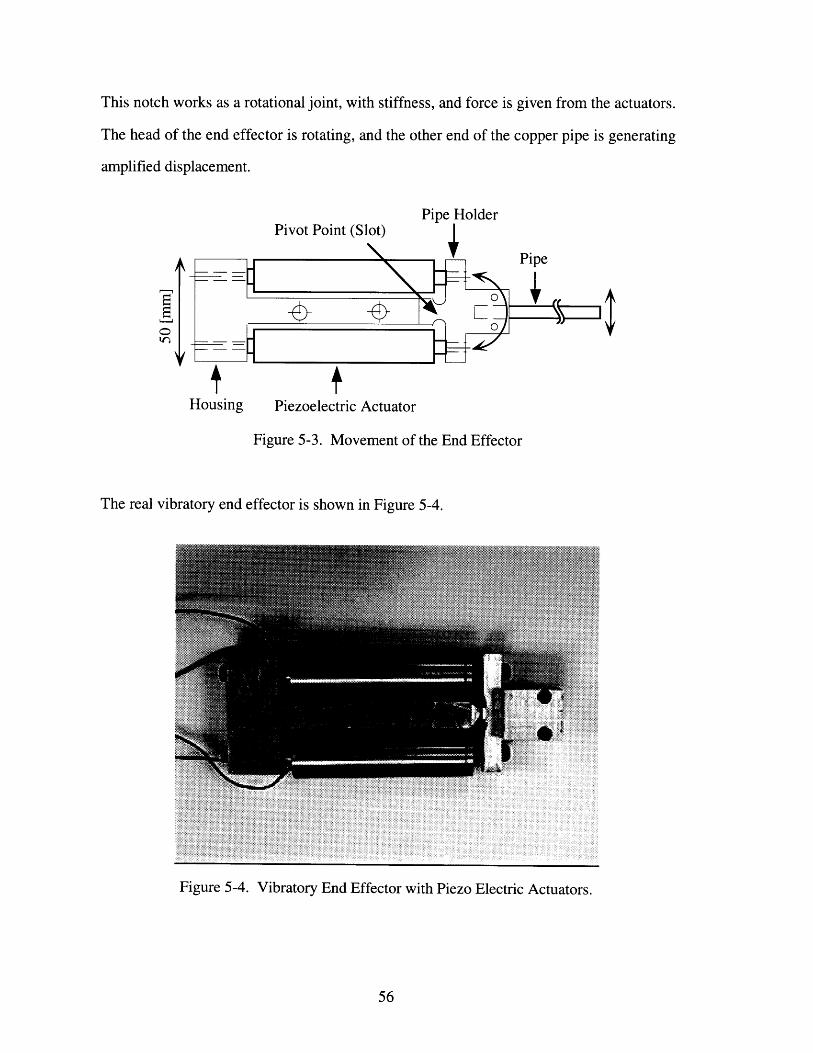
This notch works as a rotational joint, with stiffness, and force is given from the actuators.

The head of the end effector is rotating, and the other end of the copper pipe is generating

amplified displacement.

Pivot Point (Slot)Pipe Holder

Housing Piezoelectric Actuator

Figure 5-3. Movement of the End Effector

The real vibratory end effector is shown in Figure 5-4.

Figure 5-4. Vibratory End Effector with Piezo Electric Actuators.

5.3 Experimental Setup

We implemented the perturbation/correlation based controller for the insertion of a long

copper pipe into a heat exchanger. A three degree of freedom robot is controlled by a Sun

Work Station with VxWorks real time operating system. The sampling time of the control

system is 1 ms. The force sensor is mounted between the arm's endpoint and the vibratory

endeffector as shown in Figure 5-5.

Rot

Force

Figure 5-5. Vibratory End Effector Mounted on a Force Sensor

The diameter of the pipe is 8mm, the clearance is about 0.01, and aluminum foils are stuck

for inserting the pipe. The required insertion depth is 500mm. Figure 5-6 shows the

experimental setup. This piezo-electric actuators are controlled independently with the

perturbation/correlation based controller. A sinusoidal displacement command was given

to these actuators, but the force response due to this perturbation input is used to calculate

the gradient value of the performance index. This open loop controller for piezo electric

actuator followed the desired sinusoidal trajectory command with negligible phase lag,

which is important to get the correct gradient information. The three axis of the robot were

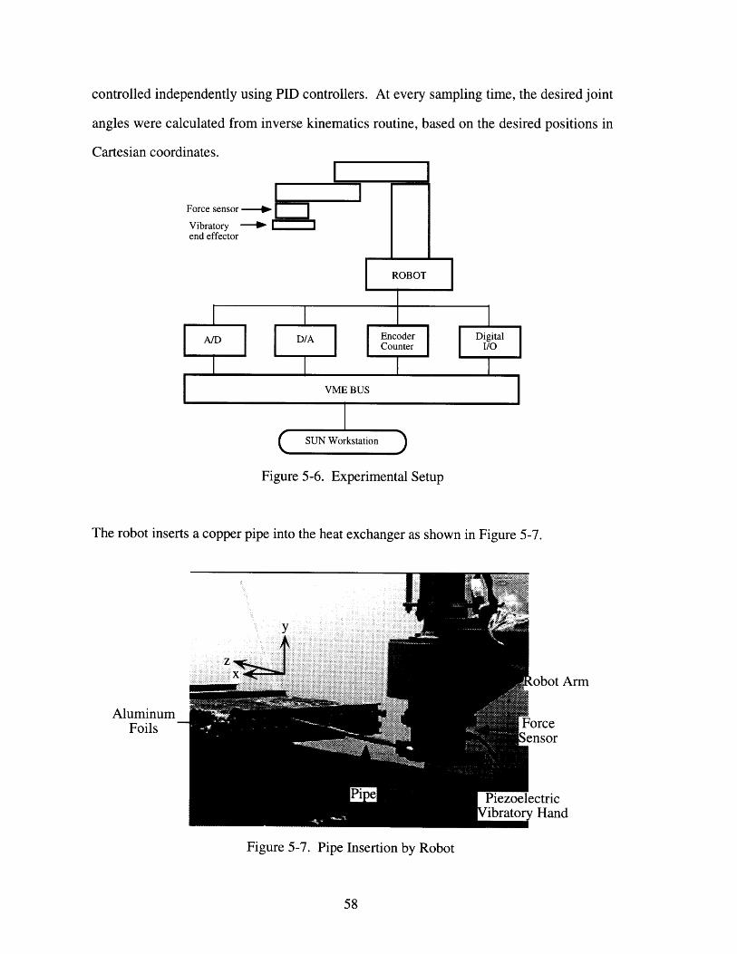
controlled independently using PID controllers. At every sampling time, the desired joint

angles were calculated from inverse kinematics routine, based on the desired positions in

Cartesian coordinates.

Force

Vibraend el

Encoder DigitalCounter I/OI I

Figure 5-6. Experimental Setup

The robot inserts a copper pipe into the heat exchanger as shown in Figure 5-7.

obot Arm

AluminumFoils )rce

nsor

ctricHand

Figure 5-7. Pipe Insertion by Robot

IA/DAM D/A

5.4 Experimental Data

Figure 5-8 shows the time profiles of the robot motion of x direction, the insertion

direction of z, the response force, Fx and the obstructing force Fz . The vibratory

endeffector was perturbed with 20 Hz in frequency. For the following one period, the

correlation was evaluated. In proportion to the resultant correlation 1 x, the x axis

command was corrected.

2 4 6[SEC]

Figure 5-8.

80

S60EE

40

20

0

1.5

1

0.5

A

8 0

2 4 6[SEC]

Fz

2 4[SEC]

Experimental Data

The x directional reference trajectories are changed in real time based on correlation value.

While generating perturbation, the input to the environment (position perturbation) and the

performance index of the system (Fz) are calculated according to the correlation equation.

Finally, the correlation value is used for updating the trajectory command. For this

experiment we focused only on minimizing the force in the z-direction.

EE

[SEC]Fx

0 6 8

i11( ,

.. ...... ... .

0drI I ' i

r7

z

........ .. ..

In chapter 3, a condition was derived for the validity of perturbation/correlation as in eq.

(5-1).j- e2 x rdF, 2;re Fz,

CO dx X=X(T) Y2 dz o =X(T).z=Z(T) Z=Z(T) (5-1)

To satisfy this condition, we use a small value of Vz and a high frequency of perturbation

o. However, it is necessary to verify this condition based on our experimental data. We

calculate the value of 3xFz on real time and use that value to update the trajectory

command. We have the values of 3xFz saved during the experiment. We can't get exact

dF.value of but we are estimating from 5xFz. In the chapter 3, we showed the measured

value of F, without perturbation, so we also get estimate of -F-. By comparing the

magnitude of zFz and 2,ie 0 d1, we can validate our assumption. Figure 5-9 shows the

values of these two under the same condition, which is with the same Vz. We can see

clearly that SxFz is more than 1000 times larger than 2 ,v0 d±= therefore the offset due to

the second term is negligible.

Vz = 10 [mm/sec]

Figure 5-9. Verification of the Eq (5-1)

5.5 Comparison with Other Force-Guided Controller

There exist many force-guided controller developed and some of them are good for

specific tasks. We need to compare the performance of this correlation/perturbation based

controller with other force-guided controllers. One of the common controller is the

compliance controller. Also, in order to check the improvement of using this vibratory end

effector, we compare with the same perturbation/correlation based controller but generating

dither by shaking the robot arm.

For the peg-in-hole insertion task, the conventional compliance controller works fine.

This controller is based on desired compliance characteristics at the entrance of the hole and

implementing joint compliance controller. However, for this pipe insertion case, the local

force information is not informative enough to guide the pipe passively and the insertion

depth is much larger. A compliance controller is designed to place the desired compliance

center at the tip of the copper pipe as in Figure 5-10.

Desired Locationof the ComplianceCenter

rxX

Figure 5-10. Compliance Center

with the following compliance values at the location of the compliance center.

61

Sc, 0cc = Cz 0 (5-2)

0 0 coo

cxx = 0.1 [m/N]

c,, = 0.001 [m/N]

coo = 0.02 [rad/Nm]

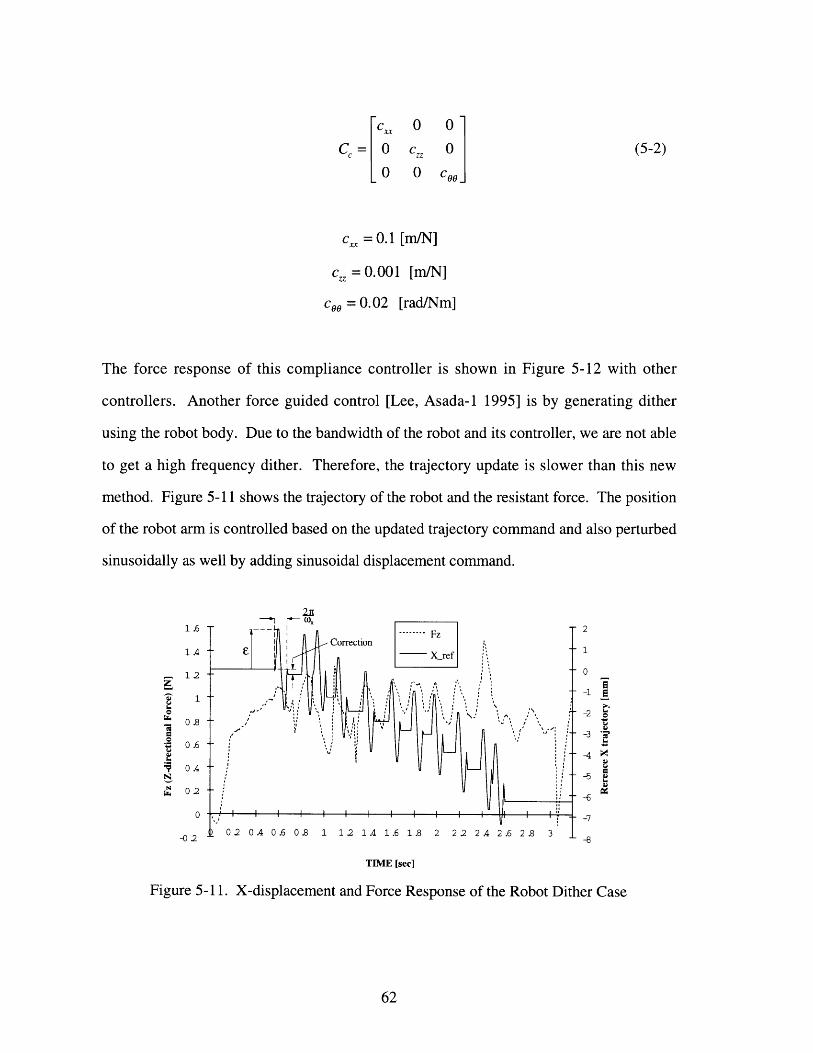
The force response of this compliance controller is shown in Figure 5-12 with other

controllers. Another force guided control [Lee, Asada-1 1995] is by generating dither

using the robot body. Due to the bandwidth of the robot and its controller, we are not able

to get a high frequency dither. Therefore, the trajectory update is slower than this new

method. Figure 5-11 shows the trajectory of the robot and the resistant force. The position

of the robot arm is controlled based on the updated trajectory command and also perturbed

sinusoidally as well by adding sinusoidal displacement command.

1 .6

1.4

12

z 1

0 .8

0 .6

• 0.4

o 02

0

2

1

0

-4

-5

-6

-7-b

TIME [sec]

Figure 5-11. X-displacement and Force Response of the Robot Dither Case

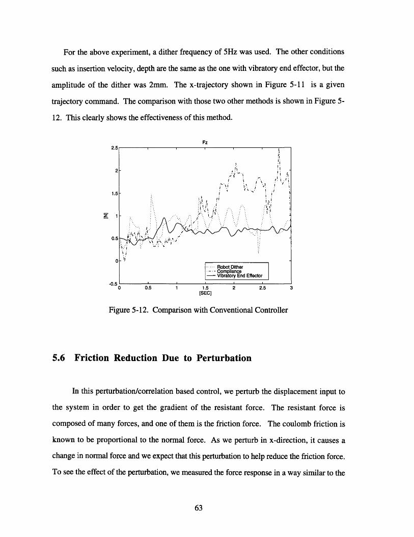
For the above experiment, a dither frequency of 5Hz was used. The other conditions

such as insertion velocity, depth are the same as the one with vibratory end effector, but the

amplitude of the dither was 2mm. The x-trajectory shown in Figure 5-11 is a given

trajectory command. The comparison with those two other methods is shown in Figure 5-

12. This clearly shows the effectiveness of this method.

Fz

1.5

...

_. Robot Dither

C- - ompliance- Vibratory End Effector

0 0.5 1 1.5 2 2.5[SEC]

Figure 5-12. Comparison with Conventional Controller

5.6 Friction Reduction Due to Perturbation

In this perturbation/correlation based control, we perturb the displacement input to

the system in order to get the gradient of the resistant force. The resistant force is

composed of many forces, and one of them is the friction force. The coulomb friction is

known to be proportional to the normal force. As we perturb in x-direction, it causes a

change in normal force and we expect that this perturbation to help reduce the friction force.

To see the effect of the perturbation, we measured the force response in a way similar to the

63

' ' 'i i

I i i

., , • . i .i

\I I? ,I

\ "• I.• II1

I~

i

A | I I I II

one in chapter 3. The difference is that we mounted the vibratory end effector on the force

sensor so that it generates a perturbation as shown in Figure 5-13.

HeatCopper Exchanger

Force sensor Pipe A01

LinearSlide

VibratoryEnd effector LII .LLIJ-z

Figure 5-13. Experiment Setup

We measured the force data as we move with constant velocity in the z-direction and

repeated several times with different x displacements. Note that the x trajectory is still fixed

and we didn't update the trajectory based on the correlation result. This experiment is

purely for estimating the effect of perturbation to reduce the friction. Same as before, we

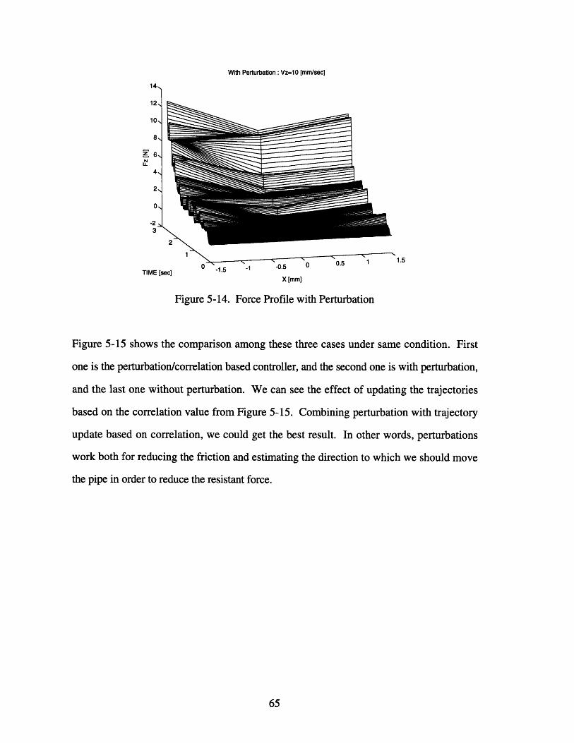
obtained similar parabolic shaped force response as shown in Figure 5-14. The magnitude

of the resistant force is much smaller than the previous case which is without perturbation.

However, this force data still shows that the minimum point of the force is not on fixed

point of x, so it is required to adjust x to reduce this force. Also, we don't know exactly

where this minimum points lies, so we need to perturb the displacement, and update the

trajectory based on the gradient value.

With Perturbation: Vz=10 [mm/sec]

14,

12,

10,

8,

Z6,

4,

2,

O0

-23

1 1.5TIME [sec] -1.5

X [mm]

Figure 5-14. Force Profile with Perturbation

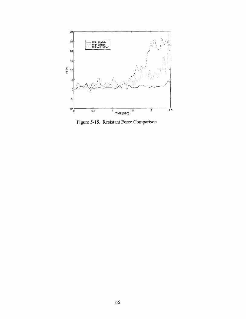
Figure 5-15 shows the comparison among these three cases under same condition. First

one is the perturbation/correlation based controller, and the second one is with perturbation,

and the last one without perturbation. We can see the effect of updating the trajectories

based on the correlation value from Figure 5-15. Combining perturbation with trajectory

update based on correlation, we could get the best result. In other words, perturbations

work both for reducing the friction and estimating the direction to which we should move

the pipe in order to reduce the resistant force.

30I

25

20

15

10U-

j

5

0

-5

1An00 0.5 1 1.5 2 2.5

TIME [SEC]

Figure 5-15. Resistant Force Comparison

-- With UpdateWith Dither I'' I

- - Without Dither7I

I

I.

0 }

. '. . . :

.. ; • .. .,•

.

__

I

Chapter 6

Application to the Connector Assembly Task

6.1 Introduction

The perturbation/correlation based control can be applied to other tasks. For a force

guided robot assembly, a performance index which represents the characteristics of the task

is selected and then a controller is made to minimize this performance index. Force

information is very essential to estimate the current state and generate new command.

However, the force from the most of the real assembly task is not informative enough to

guide the robot to accomplish the task. Especially, when the force to motion mapping is

not linear and the environment information is not well known, this perturbation/correlation

based control is a good solution. We select the connector assembly task as an example and

apply this control algorithm. Through simulation based on the analytical model, we show

the effectiveness of this approach. The comparison between this connector assembly task

and the previous heat exchanger assembly is discussed at the end.

6.2 Connector Assembly

The control method developed for the above heat exchanger assembly can be applied

to a class of tasks, where a workpiece is guided along unknown reference surfaces by

maintaining contacts with them. Consider the assembly of connectors shown in Figure 6-

1. The typical assembly process shown in the figure can be controlled in the same manner

as the heat exchanger assembly. First, the male connector held by a robot is placed on the

female connector as shown in (a), and is rotated while maintaining contacts with the female

connector as shown in (b). When the male connector comes into an upright position as

shown in (c), it is mated with the female connector and slides into the female connector (d).

During this process, the male connector is pushed against the female connector so that the

male connector can be guided along the surfaces of the female connector. The force

applied to the male connector ensures the mechanical contacts with the reference surface of

the female connector. The contact forces should be kept small, since large contact forces

create large friction which may incur stick slip when guiding along the contact surfaces.

The male connector should gently touch the female connector with small contact forces that

ensure the contacts while rotating the male connector.

(b)

(c) (d)

Figure 6-1. Connector Assembly

This control strategy for guiding the male connector can be formulated in the same

way as the heat exchanger assembly. The z axis motion in the heat exchanger assembly

indicates the depth of insertion, or the progress of assembly, and its speed is controlled

with a prescribed time function, typically a constant speed. Likewise, the rotational motion

of the male connector indicates the progress of the process, and its angular velocity is

controlled with a prescribed time function. In the heat exchanger assembly, the insertion

-- -

*1"

force F, was considered as a performance index to minimize. Likewise, the contact force

between the male and female connectors can be treated as a type of performance index : the

deviation from a desired contact force, which is small, should be minimized during the

process. Also, the friction between the two or the moment created by the friction about the

center of rotation of the male connector can be used as the performance index. In the heat

exchanger assembly, the performance index was minimized by shifting the x position. To

obtain the gradient of F, to x, a perturbation was applied to the x axis and the correlation

with F, was evaluated in order to guide the object to the minimum. Accordingly, the

performance index in the connector assembly, i.e. the contact force, is optimized through

the accommodation of x and y axes by superimposing perturbations on both axes and

evaluating the correlations. To obtain the gradient in both x and y directions, orthogonal

perturbations must be given to both axes, as will be shown in the following section.

In the connector assembly, the contact force and friction become large when the male

connector is not correctly guided along the reference surfaces of the female connector ; it

tends to move into the reference surfaces. Also, when the male connector tends to depart

from the reference surfaces, the contact for becomes lower than a specified level.

Therefore, force guided assembly in those tasks can be treated as a problem of minimizing

a performance index in terms of resistive forces. To guide a workpiece towards the

minimum of the performance index, the perturbation and correlation technique can be used

as a powerful tool. Despite noisy, erratic force signals, the perturbation/correlation method

would be able to guide a workpiece in the direction towards the optimal of a given

performance index. In the following section, the proposed method will be formally

described.

6.3 Modeling

The connector assembly task illustrated in Figure 6-1 is to correctly mate the male

connector to the female connector. Since the location of the female connector is not exactly

known, we make the male connector gently touch the female one, pressing it against and

rotating until it reaches the upright position. Based on the external forces, the

corresponding trajectory command, Vx, V, and co, can be generated based on linear

mapping. However, if there exists friction as shown in Figure 6-2, and the friction

constant is not known, the mapping is not linear anymore. We are applying the

perturbation/correlation based control to this task.

Figure 6-2. Reaction Forces

As mentioned earlier, the force is used for obtaining unknown surface information.

The goal of this task is not only assembling the connector, but also maintaining desired

contact force. In other words, we need to push the male connector to the female connector

not to lose contact, but with minimum force. Because a large normal force to the other

connector causes large friction force, thereby, we may have stick-slip and even jamming.

Therefore, our performance index is chosen as in eq. (6-3) and out goal is to minimize this

performance index while giving constant angular velocity command, o.

Fx = FxI + Fx2 (6-1)

F, = FAl - Fy2 (6-2)

P.I.=( - F,)2 +F - 1F,o)2 (6-3)

Fx'

where, Fx,o and F,,o are desired minimum force. The essential idea of this

perturbation/correlation based approach is, we perturb the current position of the center of

gravity of the male connector, and see the force response. While doing this, we estimate

the gradient of the performance index with respect to the position of the center of gravity so

that we continuously update this position based on this gradient value in order to reduce the

performance index. The coordinates of the male and the female connector are defined with

respect to the origin as in Figure 6-3. Our assumption is that the exact dimension of each

connector is known, but the position of the female connector is not exactly known.

Y

(xo,yo) L3

(0,0)

Figure 6-3. Coordinates

The exact location of the female connector, (xo,y o ) is not known, but the two points of the

male connector, (xl,yl) and (x 2 ,y2 ) can be represented with respect to the center point,

(xc 9 , 0) as shown in Figure 6-4.

(X1 ,Y1 )

(x2,y2)

Figure 6-4. Contact Points Coordinates

a = tan-' (6-4)J( (6-4)

L=2 4+L (6-5)

xi = x, - Lsin(6 + a) (6-6)

y, = yc + Lcos(6 + a) (6-7)

x2 = x + Lsin(6 - a) (6-8)

y2= Yc - Lcos(6 - a) (6-9)

Due to the stiffness of the connector, the depth of the penetration of the male connector to

the female connector is,

Ax2 =Xo + - X2 (6-10)

Ax2 = xo + L3 - x, - Lsin(O - a) (6-11)

Ay = Yo + L4 - 1 (6-12)

Ay, = yo + L4 - Yc - Lcos(6 + a) (6-13)

If we assume the wall has stiffness, Kx and K,,, which are unknown, then, the response

force would be,

F,, = KAy, (6-14)

when Ay, > 0

Fvi =0 (6-15)

when Ay1 _ 0

Fx2 = KAx2

when Ax2 > 0

when Ax2 • 0

(6-16)

(6-17)

and the coulomb friction forces with unknown friction constant, yx and py, are

Fx, = I-xFv,

Fýy2 = YyFx2

(6-18)

(6-19)

Therefore, the resultant forces are,

Fx = UxKAy, + KxAx 2

Fx = L xKv(yo + L4 - y, + Lcos(0 + a)) + Kx(x o + L - xc - Lsin(0 - a))

F, = KAy, - /1 yKx A• 2 )

F, = Ky(y o + L 4 - Yc + Lcos(0 + a))- vyKx (x o + L3 - x c - Lsin(9 - a))

(6-20)

(6-21)

(6-22)

(6-23)

The performance index, as in eq. (6-24), is

P.I.(Fx - Fxo)2+ (- F(6-24)

what we want to minimize. From the expression, we can see this performance index is

nonlinear and depends on many unknown variables.

6.4 Perturbation/Correlation based Control

The perturbations to the position of the center of the box are given orthogonally as in

eq. (6-25) and eq. (6-26)

x, = Xc o + ex sin(opt) (6-25)

yc = Yc,o + Ly cos(Opt) (6-26)

where, ex and e, are the amplitudes and o, is the frequency of the perturbation. The two

points of the box are perturbed as in eq. (6-27) through eq. (6-30)

x1 = xc,o + Ex sin(copt)- Lsin(6 + a) (6-27)

y, = yc, + ,, cos(Opt) + Lcos(8 + a) (6-28)

x2 = c,o + Ex sin(wpt)+ Lsin(9 - a) (6-29)

Y2 = Y, + ey cos(opt) - Lcos(O - a) (6-30)

For one period of the perturbation, the correlation values are calculated based on eq. (6-31)

and eq. (6-32)

f~*• xc(Pl)dT (6-31)where, 3xc = Ex sin(wopt)

S•jf +yc (PI)dT (6-32)

where, Syc = Ey cos(oWpt)

d(PI) d(PJ)so that we can estimate j-s and ,v

The center position of the box is updated based on eq. (6-33) and eq. (6-34)

,o =-_Y' at) (6-33)

P= - 7, -- (6-34)

Therefore, we can guide the box to the direction of reducing the performance index. In

chapter 3, we showed how to select the parameters. Similar analysis can be applied to this

case. The performance index in this task is defined in eq. (6-24) Let's define F as a

performance index.

F = P.I. (6-35)

The performance index F is a function of many variables.

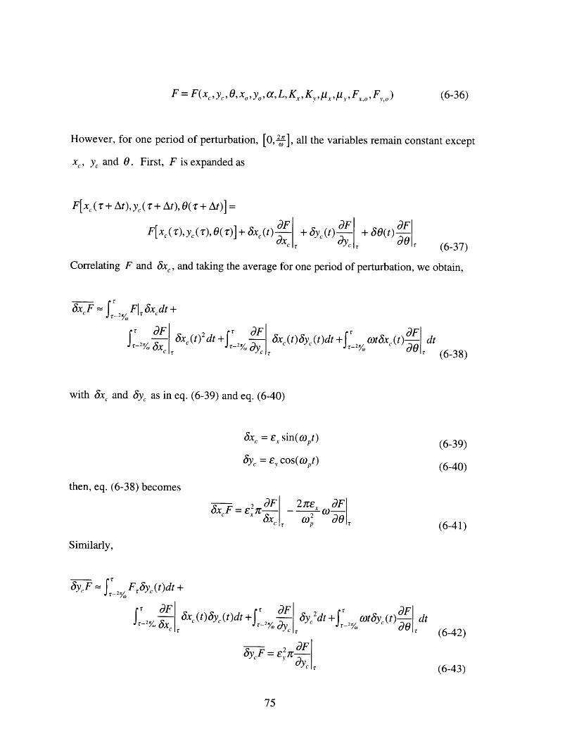
F = F(XCYC,O, xoYOa, L, Kx,K,,,x,P,,,Fx6,o,F-'o)

However, for one period of perturbation, [0,2 ], all the variables remain constant except

x,, yc and 6. First, F is expanded as

F[xc (T+ At),yc(T+ At), 0(T + At)] =

F[xc ('), yc (), 8(r)] + 3xc (t) + Sc(t) d + o(t) d

Correlating F and &3x, and taking the average for one period of perturbation, we obtain,

xcF = fr% F x&cdt+

2 xFcI Xc(t)2dt +)- 45 8X c

2 0F_ FI

S'dO L, (6-38)

with Sx& and Sye as in eq. (6-39) and eq. (6-40)

8xc = EX S

87c = E, C

then, eq. (6-38) becomes

5x cF = ex 2C X 45X&Cl

Similarly,

ycF = 2 Y F cy (t)dt +

S3~x]c(t)Syc(t)dt +f -•) & 5

dF. dyc

in(Opt)

OS((pt)

(6-39)

(6-40)

S2 -dF•W2p d r (6-41)

Syc2dt +Jl2/

dFotdy,(t) dtdO Ir (6-42)

2 dFycF = e (VKý °aYcl (6-43)

(6-37)

(6-36)

o)ts_(t)x:--xc (t)6yc (t)dt +I]_2%

Therefore to make the offset in eq. (6-41) negligible, we need a high perturbation

frequency, ,op, and a low angular velocity, o for the box.

6.5 Simulation

In order to verify this approach, a simulation was done with the following condition.

(xo,yo) = (100,100) [mm]

(x,,yc,6) = (225,190, ) [mm][rad]

S= 200, L4 = 100 [mm]

L3 = 200, L4 = 100 [mm]

Kx = 100, K, = 150 [N/mm]

lux = 0.2,,iy =0. 1

c = . [rad/sec]

p = 40tr [rad/sec]

ex = 5,e, = 5 [mm]

Yx = O.O1, = 0.01

location of the female connector

initial location of the male connector

size of the male connector

size of the female connector

stiffness of the female connector

friction constant

angular velocity of the male connector

perturbation frequency

perturbation amplitude

feedback gain

The performance index and the trajectories of xc, o and y,co are shown in Figure 6-5.

9

9

PERFORMANCE INDEX

TIME [SEC] TIME [SEC]X Y

0 1 2 3TIME [SEC] TIME [SEC]

Figure 6-5. Performance Index, X, Y and 0

We can get the gradient information which guides the male connector toward the direction

of reducing the performance index. The movement of the male connector is plotted in

Figure 6-6.

THETA

T

I

EE

MALE CONNECTORFINAL POSITION

350

300

250

200

150

100

5050 100 150 200 250

X [mm]300 350 400

Figure 6.6 Movement of the Connector

The male connector was kept rotating at the given constant angular velocity while the center

point is updated based on the control algorithm. The depth of the penetration depends on

the desired minimum force response to guarantee keeping the box contacted to the wall.

We can also select the resistant moment as our performance index, but we can not

guarantee the box contacting both side walls with that performance index.

6.6 Comparison with Pipe Insertion Task

For another application, the perturbation/correlation based control was applied to the

connector assembly task. We set up a performance index for this case and updated

variables to reduce the performance index. Based on the assumption that if we could

minimize the performance index, the task was done successfully, several key variables

which affect the performance index were selected and controlled. For the pipe insertion

FEMALE CONNECTOR

I I 1 · I 1 1 1

am-

-

-

c

I I I

case, the pipe was perturbed to see the change of the resistant force, and for the connector

assembly, the male connector was perturbed to get the change of the combined forces.

Similar approach can be used to other tasks, in which minimizing a performance index

leads to finish the task. In the pipe insertion case, the insertion speed was chosen as small

to avoid the offset term in the estimation of the gradient, and similarly, the rotation speed in

the connector assembly task. Table 6-1 summarizes the comparison between these two

cases.

Coordinate

PerformanceIndex

Perturbation

Constant Input

Control Law

3D Pipe Insertion

YvxZzF

Sx (t) = ex sin COt

Y6(t) = e, cos Wt

xd -Yx xdF.

dF.

Connector Assembly

Y

(Fx -Fx) 2 +(F, -Fo)2

45x c = Ex sin(,ot)

=yc = E cos(coPt)

d(PI)c,o =-x dxcYc,o = - y •--e

Table 6-1. Comparison Chart

Chapter 7

Conclusion

7.1 Contributions

In this thesis, a new approach for overcoming the difficulties in the force-guided

assembly for real manufacturing applications is presented. First, a performance index

which clearly represents a assembly task is chosen. We set up a goal to minimize this

performance index in order to accomplish the task. Then, we developed a way to guide the

robot to minimize this performance index. Instead of simply receiving force information

from the assembly process, we give perturbation to the robot end effector and measure the

reaction forces to the given perturbation. By taking the correlation between this

perturbation and the performance index, the reliable information for guiding the endeffector

is extracted and used for control. This small amplitude perturbation has been used for the

purpose of estimating the gradient of a performance index as well as for friction

suppression.

We generalized this perturbation/correlation based control for a robot system, and

then applied to the pipe insertion task which is difficult using the convention force guided

control Based on analytic model of this controller, Popov stability criterion is applied to

cope with the unknown nonlinearity in the environment. Several critical assumptions are

verified based on the experimental data, and the guide line to select parameters involved in

this method is presented. Both simulation and experiment, the feasibility and usefulness of

this approach are demonstrated. A vibratory end-effector using piezo electric actuator was

designed and implemented. The same control algorithm is applied to the box palletizing

task successfully.

7.1 Further Work

Some issues are still remained for further work. Even though we could get stability

condition using Popov criterion, this approach is valid only for some specific nonlinearity,

which belongs to a sector, and also for single input, single output case. More study on the

stability for other nonlinearities should be done. To apply this method for the force-guided

robotic assembly, we need to set up a performance index. This should be the one which

clearly represents the assembly task. The explicit condition for the validity of a

performance index for the assembly task should be derived. We have implemented

vibratory end effector in order to generate high frequency perturbation for the pipe insertion

task, but another methods useful for other tasks would be necessary.

Reference

[Asada and Li, 1992] H. Asada and S.-H. Li, "Automated Robotic Assembly Using a

Vibratory Work Table : Optimal Tuning of Vibrators Based on the Taguchi Method",

Proc. of the Japan-USA Symposium on Flexible Automation, Vol.2, 1992

[Cook, 1986] P. Cook, "Nonlinear Dynamical Systems", Prentice-Hall, 1986

[Eppinger and Seering, 1986] S. Eppinger and W. Seering, "On Dynamic Models of Robot

Force Control", IEEE Int. Conf. on Robotics and Automation, pp.29-34, 1986

[Erdmann, 1986] M. Erdmann, "Using Backprojections for fine Motion Planning with the

Uncertainty", Int. J. of Robitcs Research, vol.5, no.1, pp.19-45, 1986

[Hanafusa and Asada, 1977] H. Hanafusa, and H. Asada, "A Robotic Hand with Elastic

Fingers and Its Application to Assembly Processes", Proc. of IFAC Symp. on

Industrial Robots, pp.361-377, 1977

[Lee and Asada, 1994] S. Lee and H. Asada, "Assembly of Parts with Irregular Surfaces

Using Active Force Sensing", Proc. of the IEEE Int. Conf. on Robotics and

Automation, 1994

[Lee and Asada-1, 1995] S. Lee and H. Asada, "Direct Adaptive Control of Force-Guided

Assembly Using Tuned Dither", The 1995 American Control Conference, 1995

[Lee and Asada-2, 1995] S. Lee and H. Asada, "Use of Dither for Force-Guided Robot

Control", ASME International Mechanical Engineering Congress and Exposition, 1995

[McCarragher, Asada, 1993] B.J. McCarragher and H. Asada, "Qualitative Template

Matching Using Dynamic Process Models for State Transition Recognition of Robotic

Assembly", ASME Journal of Dynamic Systems , Measurement, and Control, 1993

[Narendra and Annaswamy, 1989] K.S.Narendra and A.M.Annaswamy,"Stable Adaptive

Systems", Prentice-Hall,1989

[Peshkin, 1992] M.A. Peshikin, "Admittance Matrix Design for Force-Guided

Assembly", IEEE Transactions on Robotics and Automation, Vol. 8. No.2, 1992

[Salisbury, 1980] J.K. Salisbury, "Active Stiffness Control of a Manipulator in Cartesian

Coordinates", Proc. of the 19th IEEE Conf. on Decision and Control, pp.95-100, 1980

[Sanders, Verhulst, 1985] J.A. Sanders, F. Verhulst, "Averaging Methods in Nonlinear

Dynamical Systems", Springer-Verlag, 1985

[Whitney, 1977] D.E. Whitney, "Force Feedback Control of Manipulator Fine Motions",

ASME J. of DSMC, vol.99, no.2, pp9 1-97, 1977

[Whitney, 1982] D.E. Whitney, "Quasi-Static Assembly of Compliantly Supported Rigid

Parts", Journal of Dynamic Systems, Measurement and Control, pp.65-77, 1982