A Performance Study of a Super-cruise Engine with Isothermal Combustion inside the Turbine

By

Ya-tien “Mac” Chiu

Dissertation submitted to the faculty of the Virginia Polytechnic Institute and State

University in partial fulfillment of the requirements for the degree of

Doctor of Philosophy In

Mechanical Engineering

Peter S. King, Chair

Walter F. O’Brien

Michael R. Sexton

Karen A. Thole

Uri Vandsburger

December 9th, 2004

Blacksburg, Virginia

Keywords: Cycle Analysis, Off-design Performance, Ideal Gas Mixture, Isothermal Combustion, Turbine Cooling, Super-cruise Engine

A Performance Study of a Super-cruise Engine with Isothermal Combustion inside the Turbine

Ya-tien “Mac” Chiu

Abstract

Current thinking on the best propulsion system for a next-generation supersonic cruising (Mach 2 to Mach 4) aircraft is a mixed-flow turbofan engine with afterburner. This study investigates the performance increase of a turbofan engine through the use of isothermal combustion inside the high-pressure turbine (High-Pressure Turburner, HPTB) as an alternative form of thrust augmentation.

A cycle analysis computer program is developed for accurate prediction of the engine performance and a supersonic transport cruising at Mach 2 at 60,000 ft is used to demonstrate the merit of using a turburner. When assuming no increase in turbine cooling flow is needed, the engine with HPTB could provide either 7.7% increase in cruise range or a 41% reduction in engine mass flow when compared to a traditional turbofan engine providing the sane thrust. If the required cooling flow in the turbine is almost doubled, the new engine with HPTB could still provide a 4.6% increase in range or 33% reduction in engine mass flow. In fact, the results also show that the degradation of engine performance because of increased cooling flow in a turburner is less than half of the degradation of engine performance because of increased cooling flow in a regular turbine. Therefore, a turbofan engine with HPTB will still easily out-perform a traditional turbofan when even more cooling than currently assumed is introduced.

Closer examination of the simulation results in off-design regimes also shows that the new engine not only satisfies the thrust and efficiency requirement at the design cruise point, but also provides enough thrust and comparable or better efficiency in all other flight regimes such as transonic acceleration and take-off. Another finding is that the off-design bypass ratio of the new engine increases slower than a regular turbofan as the aircraft flies higher and faster. This behavior enables the new engine to maintain higher thrust over a larger flight envelope, crucial in developing faster air-breathing aircraft for the future. As a result, an engine with HPTB provides significant benefit both at the design point and in the off-design regimes, allowing smaller and more efficient engines for supersonic aircraft to be realized.

Acknowledgement

The author would like to take a moment to recognize some of the people who have contributed to this work. I would like to thank the members of this committee for serving in this capacity. Each of you has enlightened me and expanded my knowledge and understanding on several subjects.

I would like to specially thank Dr. Peter King for his immeasurable support and instructions. By giving me free reign and timely advice, I learned more in the self-propelled, goal-pursuing way than I could ask for. I truly appreciate all the help he have provided and I feel privileged to have him as my advisor. I would also like to thank Dr. Walter O’Brien for his advice, not only on the subject matters in this research, but also on the developments in the industry of propulsion and turbomachinery. I am grateful for all the visions and information he provided as they expand my field of view and open me up to a larger world.

During the five years of my Ph.D. work here at Virginia Tech, many other have helped me and I owe them my most sincere gratitude. I would like to thank Prof. Robertshaw and Prof. Alley for their guidance and knowledge provided during our work in the class of Mechanical Engineering Lab. I would also like to thank Ben Poe and Jamie Archual for their technical support and Eloise McCoy and Cathy Hill for their administrative assistance. In addition, I must thank all of the “turbolabbers” that have walked through their graduate work with me. Their sincere friendship is one of the most rewarding parts of this journey in higher education.

Last, but not the least, I must thank my family for their support. I am especially indebted to my wife, Jennifer, for putting her own pursuit of higher education on hold and taking care of our son, Ian. She has worked tirelessly to maintain our home and raise our son so that I can devote my time on my work. Her, and Ian’s, unconditional love and support is truly what encourages me and drives me in the past five years. I could never have completed this work without them. Thank you, Jennifer and Ian.

iii

Table of Contents

Title...................................................................................................................................... i

Abstract.............................................................................................................................. ii

Acknowledgement ............................................................................................................ iii

Table of Contents ............................................................................................................. iv

List of Figures................................................................................................................... vi

List of Tables ................................................................................................................... vii

Nomenclature ................................................................................................................. viii Greek Symbols .......................................................................................................................................... x Subscripts.................................................................................................................................................. xi Engine Reference Station ....................................................................................................................... xiii Abbreviations........................................................................................................................................... xv

Chapter 1 Introduction..................................................................................................... 1

Chapter 2 Literature Review ........................................................................................... 7 2.1 Definition of a Turburner..................................................................................................................... 7 2.2 Cycle Studies on Engines with Turburner ......................................................................................... 10 2.3 Numerical Simulations on a Turburner.............................................................................................. 12 2.4 Cycle Studies on Engines with Interstage Turbine Burner ................................................................ 15 2.5 Numerical and Experimental Studies on a Miniaturized Combustor................................................. 18 2.6 Summary............................................................................................................................................ 19

Chapter 3 Modeling and Assumptions.......................................................................... 22 3.1 Engine Cycles and Configurations..................................................................................................... 22 3.2 Programming Language and Program Structure................................................................................ 26 3.3 Thermodynamic Properties of Ideal Gas Mixture in the Chosen Chemical Equilibrium Model ....... 28 3.4 Engine Component Modules ............................................................................................................. 32

3.4.1 Module for Freestream and Inlet ............................................................................................... 32 3.4.2 Module for Compressor ............................................................................................................. 34 3.4.3 Module for Isobaric Combustor................................................................................................. 35 3.4.4 Module for Turbine Coolant Mixer............................................................................................ 37 3.4.5 Module for Turbine and Turburner............................................................................................ 39 3.4.6 Module for Mixed-flow Exhaust................................................................................................. 44 3.4.7 Module for Separate-flow Exhaust............................................................................................. 47

3.5 Off-design Calculations ..................................................................................................................... 48 3.6 Validation Tests of the Program ........................................................................................................ 52

3.6.1 Simulation of a Mixed-flow Turbofan Engine ............................................................................ 52 3.6.2 Simulation of a Separate-flow Turbofan Engine........................................................................ 55

3.7 Summary............................................................................................................................................ 57 Chapter 4 Results and Discussions................................................................................ 59

4.1 Mission Requirement and Operation Limit of the Engine ................................................................. 60 4.2 Preliminary Examination of Possible Engine Configurations............................................................ 64 4.3 Cooling Flow Calculations for Different Configurations .................................................................. 73

iv

4.4 Results for Turburner Engine Optimized for Range .......................................................................... 77 4.5 Results for Turburner Engine Optimized for Size ............................................................................. 81 4.6 Sensitivity of Engine Performance to Turburner Cooling ................................................................. 89 4.7 Summary............................................................................................................................................ 96

Chapter 5 Conclusions and Recommendations............................................................ 99 5.1 Conclusions ....................................................................................................................................... 99 5.2 Recommendations............................................................................................................................ 101

5.2.1 Recommendations for Program Development ......................................................................... 101 5.2.2 Recommendations for General Turburner Research ............................................................... 103 5.2.3 Recommendations for Using Turburner Engines on Supersonic Aircraft................................ 104

Appendix A Input Data for the Cases Studied........................................................... 106 A.1 Summary of User-given Parameters, Coefficients and Efficiencies ............................................... 106 A.2 Input Data for Simulating the F101-GE-102 Engine ...................................................................... 110 A.3 Input Data for Simulating the TF34-GE-100 Engine...................................................................... 111 A.4 Input Data for Preliminary Parametric Calculations ....................................................................... 112 A.5 Input Data for Simulating the Baseline Turbofan Engine............................................................... 113 A.6 Input Data for Simulating the HPTB Engine Optimized for Range................................................ 114 A.7 Input Data for Simulating the HPTB Engine with Increased Cooling Optimized for Range.......... 115 A.8 Input Data for Simulating the HPTB Engine Optimized for Size ................................................... 116 A.9 Input Data for Simulating the HPTB Engine with Increased Cooling Optimized for Size............. 117 A.10 Input Data for Varying Cooling Flows in a Turburner ................................................................. 118 A.11 Input Data for Varying Cooling Flows in an Engine .................................................................... 119

Appendix B Engine Data Used for Validation Tests.................................................. 120

References...................................................................................................................... 124

Vita ................................................................................................................................. 127

v

List of Figures

Figure 1.1 Blackbird (left) and Concorde (right) in flight .................................................. 1 Figure 1.2 Cycle with isothermal combustion proposed by Ramohalli.............................. 2 Figure 1.3 Cycle with turburner proposed by Sirignano et al............................................. 3 Figure 2.1 Cycle with isothermal combustion proposed by Ramohalli.............................. 8 Figure 2.2 Cycle with turburner proposed by Sirignano et al........................................... 10 Figure 2.3 A schematic comparison between an engine with and without an ITB .......... 16 Figure 2.4 A comparison between the ITB cycle and the Brayton cycle ......................... 16 Figure 3.1 Detailed schematics of a twin-spool, mixed-flow turbofan engine model...... 23 Figure 3.2 Detailed schematics of a twin-spool, separate-flow turbofan engine model... 25 Figure 3.3 Structure of the cycle analysis program .......................................................... 27 Figure 3.4 Comparison between predicted and published thrust of F101 engine............. 53 Figure 3.5 Comparison between predicted and published TSFC of F101 engine ............ 54 Figure 3.6 Comparison between predicted and published thrust of TF34 engine ............ 56 Figure 3.7 Comparison between predicted and published TSFC of TF34 engine............ 56 Figure 4.1 Schematics of a twin-spool, mixed-flow turbofan engine model.................... 65 Figure 4.2 Specific thrust at supersonic cruise (BPR = 1)................................................ 67 Figure 4.3 TSFC at supersonic cruise (BPR = 1) ............................................................. 68 Figure 4.4 Specific thrust at supersonic cruise (BPR = 5)................................................ 69 Figure 4.5 TSFC at supersonic cruise (BPR = 5) ............................................................. 70 Figure 4.6 Improvement in cruise range by using HPTB engines.................................... 78 Figure 4.7 Off-design performance improvement by using HPTB engines ..................... 80 Figure 4.8 Reduction in engine size by using HPTB engines........................................... 82 Figure 4.9 Off-design performance of HPTB engines with reduced mass flow............... 84 Figure 4.10 Degradation in performance as a function of HPT cooling........................... 92

vi

List of Tables

Table 3.1 Known quantities to start simulations for a mixed-flow turbofan .................... 49 Table 3.2 Known quantities to start simulations for a separate-flow turbofan................. 51 Table 3.3 Published and predicted performances of F101 engine .................................... 54 Table 3.4 Published and predicted performances of TF34 engine.................................... 55 Table 4.1 Information on the four critical flight conditions ............................................. 61 Table 4.2 Performance comparison between different configurations (BPR = 1)............ 68 Table 4.3 Performance comparison between different configurations (BPR = 5)............ 71 Table 4.4 Performance variations caused by change in bypass ratio................................ 71 Table 4.5 Calculated parameters for turbine cooling........................................................ 76 Table 4.6 Percent reduction in engine mass flow by using HPTB engines ...................... 83 Table 4.7 Variation of throttle setting in the critical flight conditions ............................. 85 Table 4.8 Variation of bypass ratio in the critical flight conditions ................................. 85 Table 4.9 Bypass ratio variations in different flight conditions (Tt4 = 3,240 R) .............. 88 Table 4.10 Performance advantage of HPTB engines over turbofans.............................. 93 Table 4.11 Performance variation when cooling increased in different components....... 94

vii

Nomenclature

(Note: The list provided here only applies to the discussions in the main body of this dissertation. There is an additional list in Appendix A.1 that explains the variables and coefficients used in actual program.)

A Cross-sectional area

a Speed of sound

C Semi-empirical constant for calculating cooling flow

CxHy General form of hydrocarbon fuel

CO2 Carbon dioxide

Cp Specific heat

D Drag force

f Fuel-air ratio

G G-loading, 1 G = 9.81 m/s2

g G-loading, 1 g = 9.81 m/s2

H2O Water (vapor)

h Enthalpy

∆hc Heat of combustion at the standard reference state (1 atm and 298.15 K)

k Turbulence kinetic energy

L Lift force

M Mach number

MAER Expansion ratio of the cross-sectional area across the mixer

MW Molecular weight

m Mass (of a species or a gas mixture)

m Mass flow rate

cm Mass flow rate of cooling flow

gm Mass flow rate of the main hot stream

N2 Nitrogen

O2 Oxygen

P Pressure

viii

P Power

PTO Power take-out (for other devices on an aircraft)

Pi Partial pressure of species i

p Pressure

Q Rate of heat transfer/flow

R Ideal gas constant

r Radius at which the maximum tangential velocity occurs

S Flame speed

SL Laminar flame speed

s Entropy

sGEN Entropy generation through irreversibility

s Rate of entropy transfer/flow

GENs Rate of entropy generation through irreversibility

T Temperature

TBL Maximum allowable temperature of the blade

Tc Temperature of the cooling flow

Tg Temperature of the main hot stream

t Time

V Velocity of flow

V Velocity of the aircraft

Vmax Maximum tangential velocity

W Weight of the aircraft

Wfuel Weight of the fuel in an aircraft

Wpayload Weight of the payload in an aircraft

Wstructure Weight of the structure of an aircraft

Wgross Total weight of an aircraft

W+ Non-dimensional coefficient for calculating film cooling flow

w+ Non-dimensional coefficient for calculating internal cooling flow

x Mole fraction

Y Mass fraction

ix

Greek Symbols

α Bypass ratio

β Percent of core mass flow used as bleed air

ε Dissipation rate of turbulence kinetic energy

ε1 Percent of core mass flow diverted to cool high-pressure turbine/turburner

ε2 Percent of core mass flow diverted to cool low-pressure turbine/turburner

εf Film cooling effectiveness

εo Overall cooling effectiveness

η Efficiency across a component or process

η Cooling efficiency

ηm Mechanical efficiency of the shaft connecting compressor and turbine

ηmP Power conversion efficiency of devices that use the power taken off from turbine shaft

ηpc Polytropic efficiency for a compressor

ηpt Polytropic efficiency for a turbine

ηR Ram recovery factor

π Pressure ratio across a component or process

πc Overall compressor pressure ratio (including both fan and high-pressure compressor)

πf Fan pressure ratio

ρ Density

ρc Density of unburned mixture

ρh Density of burned mixture

ω Turbulence frequency

ξ Ratio between the mass flow rate of cooling flow and hot main stream

x

Subscripts

1 Reference state 1, usually the starting state of a process

2 Reference state 2, usually the ending state of a process

air Air

avg Average

b Main combustor; isobaric combustor

bypass Flow through the bypass passage

CO2 Carbon dioxide

COMP Compressor or process of compression

CV Control volume

c Compressor

comp Compressor or process of compression

comb Combustion

core Flow through the engine core (high-pressure compressor, combustor, and high-pressure turbine)

d Diffuser

f Fan

fd Bypass passage (fan duct)

fuel The property of the fuel

H2O Water (vapor)

i Index for species; index for inlet and outlet of a control volume

ideal Ideal process

in Flowing into the control volume; inlet of the control volume

M Mixer of the core and bypass flow for a mixed-flow engine

MB Main combustor

m Any mixer or isentropic mixing process

max Maximum possible value, usually occurs at ideal assumption

mix The property of a gas mixture

N2 Nitrogen

n Nozzle

O2 Oxygen

xi

out Flowing out of the control volume; outlet of the control volume

real Realist process

ref Standard reference state (1 atm and 298.15 K)

s Properties obtained through an isentropic process

T Turbine

t Total or stagnation quantity

total Total amount in a gas mixture

xii

Engine Reference Station

0 Free stream or ambient condition

1 Engine inlet or inlet to the diffuser

2 Exit of diffuser

Inlet to the fan or low-pressure compressor

3f Exit of fan or low-pressure compressor

Inlet to the high-pressure compressor and bypass passage

3 Exit of high-pressure compressor

3a Inlet to the main combustor

4 Exit of main combustor

Inlet to the coolant mixer for high-pressure turbine/turburner

4a Exit of the coolant mixer for high-pressure turbine/turburner

Inlet to the high-pressure turbine/turburner

4b Exit of the high-pressure turbine/turburner

Inlet to the interstage turbine burner

4c Exit of the interstage turbine burner

Inlet to the coolant mixer for low-pressure turbine/turburner

4d Exit of the coolant mixer for low-pressure turbine/turburner

Inlet to the low-pressure turbine/turburner

5 Exit of the low-pressure turbine/turburner

Inlet to the mixer for the core flow

Inlet to the core flow nozzle (for separate-flow engines)

5f Exit of the bypass passage

Inlet to the mixer for the bypass flow

Inlet to the bypass flow nozzle (for separate-flow engines)

6 Exit of the mixer

Inlet to the afterburner

7 Exit of the afterburner

Inlet to the convergent-divergent nozzle

8 Throat of the convergent-divergent nozzle

9 Exit of the convergent-divergent nozzle

xiii

Exit of the core flow nozzle (for separate-flow engines)

9f Exit of the bypass flow nozzle (for separate-flow engines)

xiv

Abbreviations

1-D One-dimensional

2-D Two-dimensional

3-D Three-dimensional

AB Afterburner

C-D Convergent-divergent

CFD Computational fluid dynamics

CRC Coordinating Research Council

CTT Constant temperature turbine

HPC High-pressure compressor

HPT High-pressure turbine

HPTB High-pressure turburner

IC Cases with increased cooling for turburner

ITB Interstage turbine burner

LPC Low-pressure compressor

LPT Low-pressure turbine

LPTB Low-pressure turburner

MB Main (isobaric) combustor

MTOW Maximum take-off weight

NASA National Aeronautical and Space Administration

RLV Reusable launch vehicle

RPM Revolution per minute

RTA Revolutionary turbine accelerator

TSFC Thrust Specific Fuel Consumption

TSTO Two-stage-to-orbit

UCC Ultra-compact combustor

xv

Chapter 1 Introduction

Mankind’s desire for speed has always been strong. In aviation, such desire has led us through various breakthroughs, from breaking the sound barriers decades ago to the recent success of X-43A in attaining Mach 7. Unfortunately, the technical and economical challenges associated with sustained high speed flights are tremendous and there are very few aircraft that operate in Mach 2 or above normally. In fact, there are no aircraft that have done so for more than a few flights except the venerable Blackbird and Concorde, both shown in Figure 1.1.

Figure 1.1 Blackbird (left) and Concorde (right) in flight

One of the technical challenges for sustained Mach 2 or higher flight is the performance limitation of the air-breathing engine. To maintain enough thrust in the high speed flight, the fuel consumption of the engine is so high that the aircraft has to carry a larger amount of fuel and sacrifices payload. Both Blackbird and Concorde use afterburning turbojets as propulsion source [1][2], which compare badly against the high bypass turbofans used by current jetliners. As a result of the limitation of the engine, as well as other challenges, the performances of both aircraft are overshadowed by their high operation cost and both types are retired from regular service.

With the advances in engine technology, a new generation of aircraft that can cruise at Mach 1.5 or above without using afterburner are being produced and studied now, most notable being the F/A-22A Raptor fighter for the U.S. Air Force. The requirement to quickly react to crisis is also leading the military to study a long-range strike aircraft flying at Mach 2 to Mach 4 or beyond. There are studies on space applications as well, such as the study of a Revolutionary Turbine Accelerator (RTA) by Bradley et al. [3] – an unmanned Mach 4 supersonic cruiser for use as the 1st stage of a Two-Stage-To-Orbit (TSTO) Reusable Launch Vehicle (RLV). Unfortunately, new studies on commercial applications mostly focus on business jets flying in Mach 1.5 to Mach 2 regime for the selected few, much to the disappointment of the author, who has experienced the torment of flying half way across the globe several times.

1

The reason for such lack of interest is simple. All the studies have chosen traditional turbojet/turbofan cycles with state-of-art components to propel their aircraft instead of innovative cycles that promises increased performance and efficiency. Such an approach trades the performance of the aircraft for a reduced technical challenge, but the result is that these new aircraft, if built, will face steep challenges from cheaper alternatives as the increase in performance is limited. Therefore, the new designs could only appeal to high-end market rather than mass public. In fact, even the military and space applications face challenges from cheaper alternatives such as rocket propelled missiles and launchers.

It is this author’s belief that innovative cycles should be introduced in any study that looks at developing a new supersonic aircraft. The developmental cost may be higher, but the improvement in efficiency and performance should pay off in the long run. Of all the new cycles proposed on an air-breathing engine, the author believes that using an engine with isothermal combustion in the turbine will provide the most increase in performance.

One of the studies that investigate the advantages of having isothermal combustion inside the turbine was done by Ramohalli’s [4], shown in Figure 1.2. The Brayton cycle of current turbojet and turbofan engines has four major processes, as indicated in the figure as compressor, combustor, turbine, and nozzle. Ramohalli proposed to replace the traditional combustor and turbine with a single component by introducing isothermal combustion within the turbine passages. Such a “turburner” will operate at the highest temperature achievable in a regular turbine (1800 K in the figure) and provides a 30%-40% increase in efficiency compared to traditional Brayton cycles.

0

200

400

600

800

1000

1200

1400

1600

1800

2000

6600 6800 7000 7200 7400 7600 7800

Entropy (J/kg-K)

Tem

pera

ture

(K)

Brayton Cycle Ramohalli Cycle

1

2

4

3

5

2' 4'

5'

Figure 1.2 Cycle with isothermal combustion proposed by Ramohalli

Brayton Cycle

1 2 3

4 5

Q Brayton: 1-2 Compressor 2-3 Isobaric Combustor 3-4 Turbine 4-5 Nozzle Ramohalli: 1-2’ Compressor 2’-4’ Isothermal Turburner 4’-5’ Nozzle

Ramohalli

1 2’

4’ 5’

Q

2

The auth “turburner” is a turbine th

or would like to take a moment here to clearly define that aat is designed for isothermal combustion to occur and be maintained over the

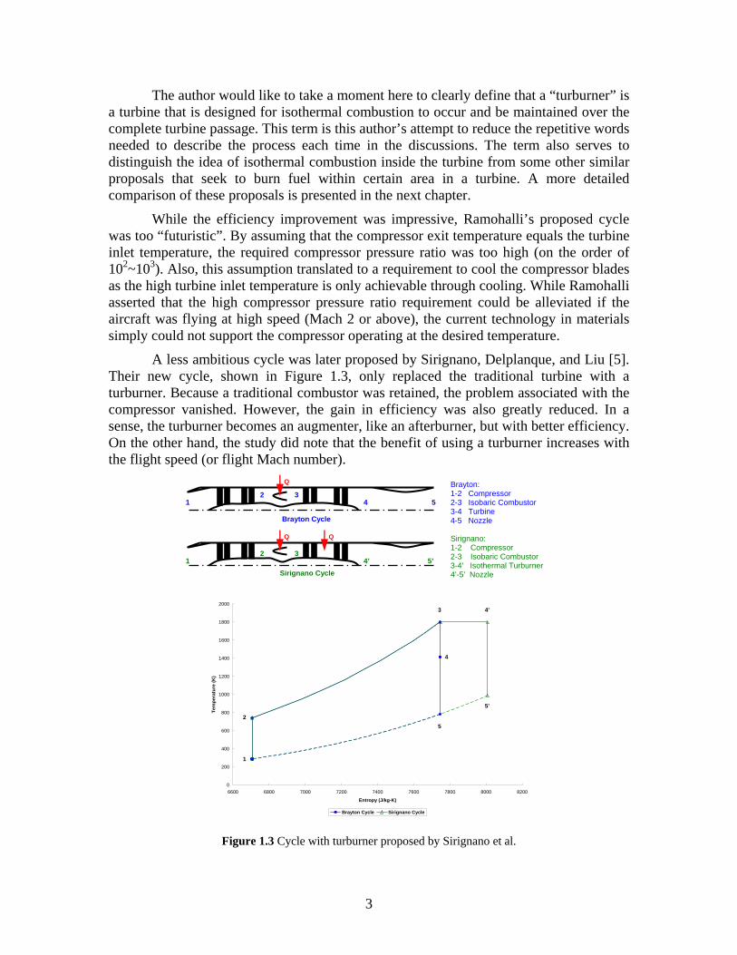
complete turbine passage. This term is this author’s attempt to reduce the repetitive words needed to describe the process each time in the discussions. The term also serves to distinguish the idea of isothermal combustion inside the turbine from some other similar proposals that seek to burn fuel within certain area in a turbine. A more detailed comparison of these proposals is presented in the next chapter.

While the efficiency improvement was impressive, Ramohalli’s proposed cycle was too “futuristic”. By assuming that the compressor exit temperature equals the turbine inlet temperature, the required compressor pressure ratio was too high (on the order of 102~103). Also, this assumption translated to a requirement to cool the compressor blades as the high turbine inlet temperature is only achievable through cooling. While Ramohalli asserted that the high compressor pressure ratio requirement could be alleviated if the aircraft was flying at high speed (Mach 2 or above), the current technology in materials simply could not support the compressor operating at the desired temperature.

A less ambitious cycle was later proposed by Sirignano, Delplanque, and Liu [5]. Their new cycle, shown in Figure 1.3, only replaced the traditional turbine with a turburner. Because a traditional combustor was retained, the problem associated with the compressor vanished. However, the gain in efficiency was also greatly reduced. In a sense, the turburner becomes an augmenter, like an afterburner, but with better efficiency. On the other hand, the study did note that the benefit of using a turburner increases with the flight speed (or flight Mach number).

0

200

400

600

800

1000

1200

1400

1600

1800

2000

6600 6800 7000 7200 7400 7600 7800 8000 8200

Entropy (J/kg-K)

Tem

pera

ture

(K)

Brayton Cycle Sirignano Cycle

1

2

4

3

5

4'

5'

Figure 1.3 Cycle with turburner proposed by Sirignano et al.

Bra on Cycle

1 4 5

Brayton: 1-2 Compressor 2-3 Isobaric Combustor

ne

ssor Combustor

rmal Turburner

yt

2 3

Q

3-4 Turbi4-5 Nozzle

QQ

Sirignano Cycle 1

2 34’ 5’

Sirignano: 1-2 Compre-3 Isobaric 2

3-4’ Isothe4’-5’ Nozzle

3

From the st tilizing a turburner shows great prom

engine with a turburne

ad investigated this matter with approxim

tailed performance analysis is needed to first

udies mentioned above, one can see that an engine uise in propelling a supersonic aircraft. In fact, even Ramohalli’s cycle is

not entirely impossible if it is used on expendable applications such as missiles, where the material only has to withstand high temperature in a very short amount of time1. However, there are many technical challenges associated with maintaining combustion in the turbine passage. The effort and researches that followed these two works started to diverge into focusing on the details of these technical issues and no attention was paid on a more detailed performance analysis.

Of course, any technical challenge has to be resolved and understood before an r could be built, but the problem in diving into details immediately

is that we may be tackling a technical challenge that does not exist. For example, whether the combustion could be maintained in the flow environment of a turbine was open to debate at the time of the two studies mentioned above.

Several experimental and numerical studies hated geometry and flow conditions based on current turbine. The results

definitely showed that a turburner based on current turbine is possible and certainly were great encouragements for anyone who is interested in making turburner a reality, but what if employing a turburner engine on certain applications demanded an entirely different turbine design or flow conditions?

It is the belief of this author that a deidentify what kind of applications will benefit the most from using a turburner engine. With a particular application identified, researchers will have a clearer picture of what specific issues need to be addressed to produce an engine for such use. As a result, research effort could be focused on these issues and fewer resources are needed to develop such an engine.

An example of this approach is applying Ramohalli’s cycle in a missile engine mentioned earlier. For an aircraft engine, his cycle is simply a no-go as there is no technology to build the required compressor with enough fatigue life. For a missile engine, the requirement in fatigue life is greatly reduced. Also, the engine cycle in a missile usually does not operate in a temperature as high as an aircraft engine, so the required compressor pressure ratio is lowered. Finally, if the missile is designed for supersonic speed, which is the norm for current missiles, the required compressor pressure ratio will be lowered further because of the ram air effect. With the combined effect of these three factors, Ramohalli’s cycle certainly becomes a possibility and, in fact, a very attractive engine choice for a supersonic missile.

On the other hand, as an expendable application, minimizing the cost of each missile is also very important. Therefore, the merit in performance of using a turburner engine must be weighted against the cost of using the new technology. As a result, detailed analysis that provides accurate estimate of engine performance using different engine parameters and known technology limits is needed. The performance prediction could then be used with cost estimation to define the best turburner engine configuration for this application. Further researches will focus on resolving the technical challenges of

1 The life of a missile engine typically spans from several hours to ten or twenty hours. On the other hand, the life of an aircraft engine is at least a thousand hours.

4

this particular engine configuration first. Once the technology has matured in one particular application, future work can build on the experiences learned and spiral out to different applications.

Unfortunately, no study has been done with a specific application and mission requirement in mind to identify the real performance gain of using a turburner engine. All the cyc

ions involve engines

rly unacce

proprietary to engine

alysis on a turburner engine and other innovative cycles. This program will be used to

The details of the models and assumptions used in the cycle analysis program

le studies2 that have been done focused on generic trend of the performance. As a result, simplified assumptions such as calorically perfect gas and ideal component efficiency were used. Also, important engine parameters, such as the amount of cooling (which could affect the performance dramatically), were not modeled at all.

In addition to these basic assumptions that limit the accuracy of the results, most works done so far only performed on-design cycle analyses. Realistic miss

running at off-design conditions, so a promising on-design cycle may not satisfy real world mission requirements. To truly understand how well a turburner engine compares to a regular turbojet or turbofan, off-design performance must be evaluated.

In order to identify the best turburner engine configuration for a particular application, the uncertainty associated with the simplified assumptions is clea

ptable. Furthermore, off-design performance must be calculated in addition to the on-design performance. Therefore, a performance study that is similar to the trade-off studies in the preliminary design stage of a real world engine is needed.

However, there is no tool available that could perform such analysis with the desired details and accuracy. Programs with such capability are usually

manufacturers and are difficult to obtain the right to use. Furthermore, these programs are designed with the current engines in mind and sometimes use experimental data extensively, making them hard to be used directly or modified to study innovative cycles.

Therefore, this study aims to develop a program to perform accurate and detailed cycle an

demonstrate the benefit of using a turburner engine in a supersonic cruising aircraft. The program could then be used with other airframe design tools to find the optimum design of an airframe/propulsion combination for a particular mission need. Another desired attribute of the program is the potential to be easily modified to study other cycle concepts in order to address the need for a tool to analyze new cycle concepts in greater details. It is hoped that the new tool and the analysis could lead to more focused researches on supersonic aircraft and turburner engines (or any other new cycle concept), therefore expedite the developmental work and reduce the cost of the new technology.

In the next chapter, literature regarding turburner cycles and other related research is presented.

are then presented in Chapter 3, along with results from validation tests of the new code. In Chapter 4, the predicted performance of using a turburner engine in a

2 There are several other cycle studies on a turburner engine or other similar concepts. The details of these studies are presented in the next chapter. However, they all use the same assumptions discussed here.

5

supersonic aircraft and the benefits of doing so are discussed. Then, conclusions and recommendations are presented in Chapter 5.

6

Chapter 2 Literature Review

The concept of introducing isothermal combustion within a turbine is not really new, but the studies on cycles using such technology are certainly few. The earliest literature accessible is Ramohalli’s work [4] mentioned previously, dated 1987. Afterwards, there is a blank between Ramohalli’s study and the study by Sirignano et al. [5] for nearly ten years. Fortunately, there are several studies that followed, either studying more on the cycle performance or simulating numerically the flow and combustion in a turburner.

On the other hand, there is a separate effort in miniaturizing the traditional combustor. This effort led to several designs that use a highly-swirled flow environment to enhance combustion, thereby reducing the size of the combustor. Such flow environment is somewhat similar to the flow in a turbine, so the results could be applied to a turburner cycle. In fact, using one such miniature combustor between the high-pressure and low-pressure turbine sections to creating an Interstage Turbine Burner (ITB) was even proposed and studied. The idea is certainly similar to the turburner and worth discussing, if not just for the purpose of clarifying the differences between the two cycles.

In this chapter, the concept of a turburner is first discussed in greater details than what have been presented in Chapter 1. Then, cycle studies on an engine with turburner are presented, followed by several studies that performed numerical simulations on a turburner. A discussion on cycles such as ITB cycle and some comparisons between different cycles are presented next. Then, both experimental and numerical research on miniaturizing the combustor is presented. A summary of important observations from the presented literatures is shown at the very last to conclude this chapter.

2.1 Definition of a Turburner

As defined in the previous chapter for this research, a turburner is a turbine that is designed for isothermal combustion to occur and be maintained over the complete turbine passage. Unlike the combustions sometimes occurring in the turbine of current engines, which are the “left-over” combustion from the main combustor, a turburner is designed with proper fuel injection and flame holding mechanism to maintain a controlled combustion throughout the turbine stages. In fact, the combustion must be controlled precisely to get as close to an ideal isothermal process as possible.

The idea of having isothermal combustion in the turbine to improve efficiency comes directly from the First Law of Thermodynamics for a cyclic process. To maximize the work output, the heat addition should take place at the highest allowable temperature while the heat removal should be done at the lowest allowable temperature for any thermodynamic cycle. However, heat addition inevitably leads to temperature increase, so either work extraction is needed to maintain the temperature or the cycle has to start the heat addition process at a lower temperature. Adding the two requirements together, it

7

is quite obvious that a turbine with proper amount of heat addition (through combustion) could create an isothermal process and maximize the cycle performance.

The concept of a turburner can be more easily understood through visualization of a sample thermodynamic cycle. As briefly discussed in Chapter 1, the earliest analysis on a cycle using a turburner is done by Ramohalli [4]. The cycle plot has been shown earlier, but is repeated here in Figure 2.1 as an example3.

0

200

400

600

800

1000

1200

1400

1600

1800

2000

6600 6800 7000 7200 7400 7600 7800

Entropy (J/kg-K)

Tem

pera

ture

(K)

Brayton Cycle Ramohalli Cycle

1

2

4

3

5

2' 4'

5'

Figure 2.1 Cycle with isothermal combustion proposed by Ramohalli

In the figure, an ideal Brayton cycle is defined by the blue line of 1-2-3-4-5 and includes four processes: a compressor, a combustor, a turbine, and a nozzle4. Because it is assumed to be ideal, the combustion process is isobaric (pressure at 2 equals to pressure at 3) and all other processes are isentropic. 3 The author would like to point out that this plot and other plots in this chapter only serve as examples for the readers to understand the differences between each cycle. Therefore, these plots are generated without any consideration to the property variations caused by the energy release and the mass transfers during the combustion. The plots, however, are generated with thermally perfect gas model instead of the calorically perfect gas model used by other studies. In other words, specific heat and other thermodynamic properties do vary with temperature. 4 Sometimes a nozzle is not included in the discussion of simplified thermodynamic cycles. Since only thrust engines are studied in this research (even though the program can be adapted to other applications), the nozzle is included to better distinguish the isentropic expansion through a turbine from that of through a nozzle.

Brayton Cycle

1 2 3

4 5

Q

Brayton: 1-2 Compressor 2-3 Isobaric Combustor 3-4 Turbine 4-5 Nozzle Ramohalli: 1-2’ Compressor 2’-4’ Isother al Turburner m4’-5’ Nozzle

Ramohalli Cycle

1 2’

4’ 5’

Q

8

On the other hand, the Ramohalli cycle is defined by the green line of 1-2’-4’-5’, with a much higher compression ratio than that of the Brayton cycle and a turburner that replaces both the combustor and turbine of the Brayton cycle. The turburner is represented as process 2’-4’, forming a horizontal line in the T-s diagram, which represents an isothermal process.

Clearly, Ramohalli’s cycle produces much more work than a Brayton cycle as the area encircled by the green line in the T-s diagram, which signifies the work output as stated in the First Law of Thermodynamics, is much larger than the area encircled by the blue line. For a thrust engine, the kinetic energy of the exhaust is also much greater because the height of line 4’-5’ is much greater than the line 4-5, which translates to more expansion or more enthalpy being converted to exhaust velocity in the nozzle.

Another interesting fact is that the entropy generation for a turburner is less than that of a traditional combustor because the heat addition takes place at a higher temperature, as stated by the Second Law of Thermodynamics,

CV iin out

i i CV

ds Qs sdt T

⎛ ⎞≥ − + ⎜ ⎟

⎝ ⎠∑ ∑ ∑ (2.1)

where CVdsdt

is the rate of change of the entropy in a control volume, is the entropy

flow entering the control volume, is the entropy flow leaving the control volume, and

ins

outs

i

i CV

QT

⎛ ⎞⎜ ⎟⎝ ⎠

is the heat transfer into the control volume in a constant temperature. This

reduction in entropy generation moves the 4’-5’ line to the left of the 4-5 line and increases the thrust slightly.

A closer examination of Figure 2.1 and the Second Law may lead some readers to question whether the process in a turburner is truly isothermal, or more precisely, whether it is the static temperature or the total temperature that is being held constant. By definition, isothermal process is a process that the temperature does not change and the temperature can certainly be either static or total in a theoretical analysis. The Second Law, however, shows that maximizing static temperature is needed to minimize the entropy generation, so ideally the static temperature should be maintained constant in a turburner.

Unfortunately, given the complex flow environment in the turbine, maintaining a uniform static temperature field through out the entire blade passage is almost, if not entirely, impossible to achieve in reality. It is also hard to enforce such a condition in a non-dimensional cycle analysis because velocity information is needed to find the static temperature. As a result, Ramohalli and all other works studying a turburner cycle, including this research, assumed constant total temperature as the isothermal process in a turburner.

Assuming ideal components and using calorically perfect gas model, Ramohalli showed that the proposed cycle provides a 30% to 40% increase in efficiency over the Brayton cycle. However, the cycle not only required the design of a turburner – a

9

complete turbine section designed to operate in high temperature of the combustion while maintaining the aerodynamic performance – that operates in higher pressure than then-current engines, but also a compressor that could compress the air to a high temperature and pressure level previously unheard of. In fact, for Ramohalli’s cycle shown in Figure 2.1 with standard atmospheric air inlet at sea level and a turbine inlet total temperature of 1800 K, the compressor pressure ratio is about 1,100. Consequently, the study did not generate many followers and still remained as the only literature studying this cycle.

On the other hand, the merits of combining the combustion and the turbine expansion processes to form a new isothermal combustion process had been demonstrated. If done properly, the isothermal combustion process is vastly superior to the traditional setup of an isobaric combustion followed (or preceded) by an isentropic expansion. As a result, while the exact same cycle proposed by Ramohalli had not been followed, the studies on creating a turburner and using a turburner in other innovative cycles continued.

2.2 Cycle Studies on Engines with Turburner

Sirignano, Delplanque, and Liu [5] proposed a much less ambitious cycle that employs a turburner, shown in Figure 2.2. In the figure, the traditional Brayton cycle is represented in blue, composing of four major processes, while the proposed cycle is shown in green, also composing of four major processes. The isothermal turburner is represented in the T-s diagram as the horizontal line 3-4’.

0

200

400

600

800

1000

1200

1400

1600

1800

2000

6600 6800 7000 7200 7400 7600 7800 8000 8200

Entropy (J/kg-K)

Tem

pera

ture

(K)

Brayton Cycle Sirignano Cycle

1

2

4

3

5

4'

5'

Figure 2.2 Cycle with turburner proposed by Sirignano et al.

Brayton Cycle

1 2 3

4 5

Q Brayton: 1-2 Compressor 2-3 Isobaric Combustor 3-4 Turbine 4-5 Nozzle Sirignano: Q Q1-2 Compressor 2-3 Isobaric Combustor 2 3 3-4’ Isothermal Turburner 1 4’ 5’4’-5’ Nozzle

Sirignano Cycle

10

Obviously, the most distinctive feature of the proposed cycle is that a traditional isobaric combustor is maintained. The result is that both cycles present very similar profile in the T-s diagram. In fact, one can clearly see that the only increase in work output of the proposed cycle when compared to the Brayton cycle comes from the right most area, encircled by the line 3-4’-5’-5.

In a sense, the turburner combines the function of a turbine and an afterburner, with better efficiency. The efficiency improvement comes from the fact that a traditional afterburner still goes through an isobaric combustion, which leads to less work output and more entropy generation when compared to an isothermal combustion.

Using a calorically perfect gas model and assuming ideal component efficiencies, Sirignano et al. showed that their cycle could provide 10%-15% increase in specific thrust over a non-afterburning Brayton cycle. They also noted that the benefit of using a turburner increases with the flight speed (or flight Mach number). Land-based gas turbine generators were studied as well and similar increase in performance was demonstrated.

Liu and Sirignano [6] later expanded the work to include single-shaft, separate-exhaust turbofan engines, using procedures outlined in Hill & Peterson [7]. Their work showed that an engine using their proposed cycle had a distinct advantage over current engines, with or without afterburning. As the engine compressor pressure ratio increased, the performance of their proposed turburner cycle increased while the performance of both afterburning and non-afterburning Brayton cycle actually decreased. They asserted that such trend would enable their cycle to provide superior performance at high speed because the ram air compression would boost the overall compression to a higher level.

A separate effort by Andriani et al. [8] also investigated the performance increase of a turbojet engine with a Constant Temperature Turbine (CTT), which was exactly the same as the cycle proposed by Sirignano et al. discussed above. The models and assumptions used were the same as what Sirignano et al. had used, so the results were very similar as well. However, Andriani et al. did attempt to address the off-design performance of their cycle by deriving a basic model. The model was derived by assuming that the flows at the inlet to the turbine and at the throat of the nozzle are choked. The resulting formula established compressor pressure ratio as function of engine inlet conditions, turbine inlet temperature, and the area ratio between the throat of the nozzle and the inlet to the turbine.

Andriani and Ghezzi [9] then performed several calculations to demonstrate the feasibility of applying their model to find off-design performance of a turbojet engine with a turburner. However, the results did not include a base case, such as a regular turbojet, for comparison, so no conclusion was drawn about how much performance could be gained in off-design conditions. On the other hand, they did conclude that if the area ratio between the throat of the nozzle and the inlet to the turbine could be varied in certain flight conditions, it would provide significant increase in performance over a turburner engine with fixed geometry.

From these studies, it is quite clear that an engine using the turburner cycle proposed by Sirignano et al. provides a good alternative to a turbojet with afterburner, especially for high speed flight. Because a traditional combustor was retained, the problem associated with the required large compressor in Ramohalli’s cycle was

11

addressed. The turburner was also operating at a pressure very similar to current turbines – Ramohalli’s cycle demanded the turburner to operate in a much higher pressure – so overall the technical challenges was much smaller.

On the other hand, the performance increase was not as impressive as Ramohalli’s futuristic cycle. Considering that all the studies assumed ideal components and used calorically perfect gas model, the 10%-15% performance improvement demonstrated became questionable. Granted, all the turbojets or turbofans used as baseline were also ideal, but one would expect the component efficiency of the new cycle to be lower than the current state-of-art turbine engine simply because the cycle is new and not enough experience and knowledge has been accumulated.

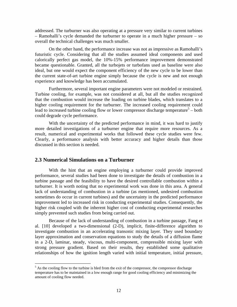
Furthermore, several important engine parameters were not modeled or restrained. Turbine cooling, for example, was not considered at all, but all the studies recognized that the combustion would increase the loading on turbine blades, which translates to a higher cooling requirement for the turburner. The increased cooling requirement could lead to increased turbine cooling flow or lower compressor discharge temperature5 – both could degrade cycle performance.

With the uncertainty of the predicted performance in mind, it was hard to justify more detailed investigations of a turburner engine that require more resources. As a result, numerical and experimental works that followed these cycle studies were few. Clearly, a performance analysis with better accuracy and higher details than those discussed in this section is needed.

2.3 Numerical Simulations on a Turburner

With the hint that an engine employing a turburner could provide improved performance, several studies had been done to investigate the details of combustion in a turbine passage and the feasibility to have the desired controllable combustion within a turburner. It is worth noting that no experimental work was done in this area. A general lack of understanding of combustion in a turbine (as mentioned, undesired combustion sometimes do occur in current turbines) and the uncertainty in the predicted performance improvement led to increased risk in conducting experimental studies. Consequently, the higher risk coupled with the inherent higher cost of conducting experimental researches simply prevented such studies from being carried out.

Because of the lack of understanding of combustion in a turbine passage, Fang et al. [10] developed a two-dimensional (2-D), implicit, finite-difference algorithm to investigate combustion in an accelerating transonic mixing layer. They used boundary layer approximation and conservation equations to study the details of a diffusion flame in a 2-D, laminar, steady, viscous, multi-component, compressible mixing layer with strong pressure gradient. Based on their results, they established some qualitative relationships of how the ignition length varied with initial temperature, initial pressure,

5 As the cooling flow to the turbine is bled from the exit of the compressor, the compressor discharge temperature has to be maintained in a low enough range for good cooling efficiency and minimizing the amount of cooling flow needed.

12

initial velocity, transport properties, and pressure gradient. They also concluded that both oxidation kinetics and transport were controlling the ignition region while only the transport was controlling the fully established flame.

The work on laminar flow by Fang et al. was later extended to include the Baldwin-Lomax turbulence model by Cai et al. [11]. Using the finite-volume method, a compressible Navier-Stokes equations solver with chemical reaction was developed without using the thin mixing layer assumption. The solver was used to simulate the ignition and combustion in a turbulent flow within a curved-duct subject to both axial and traverse pressure gradient. Several curved-ducts with different geometries, including one with pronounced cross-sectional area change that represented a turbine passage more closely, and different fuel injection points were studied. The results showed that traverse pressure gradient had little effect on the flame structure, except through the induced non-uniform velocity field that created a thicker flame in low speed region. However, the combustion was actually enhanced as the flow temperature was higher when the flow was subject to traverse pressure gradient.

The studies of simplified duct flow presented above provided insight into the flame structure in a flow with strong pressure gradient and demonstrated that it was feasible to maintain combustion in such environment. However, the simplified geometry could not capture some of the flow characteristics in a real turbine passage because of several missing features, such as the fuel injection mechanism and the rotor-stator interactions. As a result, several other CFD (Computational Fluid Dynamics) studies were carried out to simulate the combustion in a turbine passage by modeling blade cascades.

Nagumo et al. [12] performed a full 3-D (three dimensional), Reynolds-averaged Navier-Stokes simulation with k-ε turbulence model on a vane cascade6 to investigate the effect of blade geometry on combustion. The study assumed that gaseous hydrogen was injected through the film cooling holes on the suction side of the vanes. This assumption not only addressed the lack of a physical fuel injection mechanism in other studies, but it also provided a potential solution to the question regarding increased cooling requirement for a turburner.

The results from the study by Nagumo et al. provided an insight into the 3-D structures of the combustion and flow field along the blade passage. It was alsoshown that unburned fuel near the blade surface indeed shielded the blade from the dramatic increase in temperature of the main flow and provided film cooling for the blade just like cooling air7. On the other hand, they noted that the aerodynamic performance of the blade was degraded, as the pressure on the suction side of the vanes increased with the combustion.

Isvoranu and Cizmas [13] developed a Reynolds-averaged Navier-Stokes code that incorporated a two-step combustion mechanism to study the effect of rotor-stator

6 The profile of the vanes was modeled after the vanes of the turbine in a GE90 engine. 7 Because the simulation was carried out over a vane or stator cascade, no work extraction took place and the temperature of both the main flow and the blade were allowed to increase. However, temperature increased at a much slower rate on blade surfaces subject to a thin film of unburned hydrogen than anywhere else.

13

interaction on the combustion inside a turbine. The computational domain was a full turbine stage cascade that included thirty two periodical sub-domains, each with a stator injecting methane fuel at its trailing edge, followed by a rotor rotating at 3,600 RPM. The results showed that while combustion could be maintained in the flow field of a turbine, the large unsteadiness of the flow and the wide range of variation in velocity led to a wide spread of local time scales that affected the reaction. As a result, temperature non-uniformities in a turburner would be quite different and more severe than a traditional turbine, requiring even more detailed studies to determine the effect on the loading of the blades and the optimum cooling scheme.

Another CFD study on a full turbine stage cascade was done by Rice [14]. Unlike the other studies presented in this section, Rice used the commercially available software FLUENT instead of developing his own algorithm. In addition to the built-in k-ω turbulence model and single-step chemical reaction of FLUENT, the study also investigated two different approaches to model the turbulence mixing and the effect on the results. Several injection schemes for the JP-8 fuel, such as injecting at the leading edge of the suction side of the stator, were also tested to investigate the effect of injection placement on the combustion and the aerodynamic performance of the blade.

The computational domain included a stator followed by a rotor with tangential velocity of 275 m/s, corresponding to roughly 5,250 RPM for a turbine rotor with a 0.5 m radius or 8,750 RPM for a rotor with a 0.3 m radius. This rotational speed was significantly higher than any other studies had simulated and represented a much closer approximation of the flow within a turbine.

Rice’s results showed that the combustion for a typical aviation hydrocarbon fuel8 within an environment very similar to a turbine was self-igniting and self-sustaining. Temperature non-uniformities were more severe than a turbine without combustion, especially when the fuel was injected on the pressure side of the rotor. To minimize non-uniform thermal pattern, injecting fuel on the leading edge of the suction side of the rotor was recommended. Also, there did not appear to be noticeable aerodynamic penalties on the performance of the rotor blades, unlike what Nagumo et al. had concluded. Rice suggested that the difference may have been caused by the difference in the amount of heat release between the two studies, as the amount of fuel injected in his study was very small in order to maintain the overall process to be as close as isothermal.

From the studies presented, it is quite clear that isothermal combustion inside a turbine passage, while quite complicated and a lot still needs to be investigated, is not impossible to achieve. Although the results are still not comprehensive enough to guarantee that combustion within an arbitrary turbine passage with any inlet conditions could always be maintained, cases that closely represent current turbines have shown promising results.

On the other hand, the studies may have raised more questions regarding how to design a turburner than before. For example, the observed temperature non-uniformities may require additional cooling flow to the turbine unless innovative cooling schemes 8 It is worth noting that the JP-8 fuel used in Rice’s simulations is not only widely used in the military in itself, it is also almost identical, with the exception of a few additives, to the Jet-A fuel used in commercial jetliners.

14

such as using unburned fuel to provide film cooling can be realized. Unfortunately, the addition of cooling air was not modeled in the cycle studies of previous section nor any of the numerical studies in this section. A detailed cycle analysis that models the cooling flow is certainly most useful in this situation to ascertain how much cooling flow a turburner can afford before overall performance is reduced to below the performance offered by turbofan. The results can then be used to guide other numerical or experimental work to determine whether the amount of cooling is enough to maintain the integrity of the blades.

2.4 Cycle Studies on Engines with Interstage Turbine Burner

As mentioned in the beginning of this chapter, separate efforts in miniaturizing combustors have also produced several results relevant to the idea of a turburner. In fact, these efforts have led to a concept temporarily named Interstage Turbine Burner (ITB). Just for the purpose of clarification alone, the concept of ITB has warranted its place in this review of literatures. Another important reason to discuss this concept is the fact that the program developed in this research can simulate the ITB cycle and has actually been used to simulate this cycle – not only to demonstrate the capability of the program but also to investigate the advantage of a turburner cycle over an ITB cycle.

The name Interstage Turbine Burner was coined by Siow and Yang [15] to describe the miniature combustor in the transition duct between a high-pressure turbine section and a low-pressure turbine section. It should be noted that all the other cycle studies presented so far assumed a single-spool engine, where all the compressor stages were driven through a single shaft by all the turbine stages. On the other hand, an engine with an ITB has to have at least two spools9: the fan (or low-pressure compressor, LPC) is driven by the low-pressure turbine (LPT) in one spool while the high-pressure compressor (HPC) is driven by the high-pressure turbine (HPT) in another spool. A schematic comparison between a twin-spool engine with an ITB and without an ITB is shown in Figure 2.3.

9 There are single-spool, ground-based gas turbine generators that add isobaric combustors between turbine stages. Theoretically, miniature ITB can also be used in a single-shaft, multi-stage turbine of an aircraft engine. However, all the studies on aircraft engine with an ITB center on applying the ITB to between the HPT and LPT, possibly in order to avoid degrading the operability of the engine.

15

Brayton:

Figure 2.3 A schematic comparison between an engine with and without an ITB

One can clearly see from Figure 2.3 that there exist two compressor sections, each driven by one turbine sections. The ITB is placed between the two turbine sections, so the heat addition process is purely isobaric, exactly the same as the main combustor. Consequently, an ideal ITB cycle will look very much like a Brayton cycle with afterburner, as evidenced in Figure 2.4.

0

200

400

600

800

1000

1200

1400

1600

1800

2000

6600 6800 7000 7200 7400 7600 7800 8000 8200

Entropy (J/kg-K)

Tem

pera

ture

(K)

Brayton Cycle Interstage Turbine Burner Cycle

1

2a

2

3

4a

4

5

4b

4'

5'

Figure 2.4 A comparison between the ITB cycle and the Brayton cycle

For readers familiar with the cycle representation of an afterburning turbojet in a T-s diagram, the ITB cycle shown in Figure 2.4 will look strikingly similar to a Brayton cycle with afterburner. The only telltale sign are the station numbering that indicates the isentropic process 4b-4’ is actually the low-pressure turbine (instead of an ideal nozzle) and the fact that the highest temperature in the cycle is only 1,800 K – typical for the highest temperature allowed in a turbine passage, but much lower than the normal temperature in an afterburner.

Brayton: 1-2a Fan/LPC 2a-2 HPC 2-3 Combustor 3-4a HPT 4a-4 LPT 4-5 Nozzle ITB: 1-2a Fan/LPC 2a-2 HPC 2-3 Combustor 3-4a HPT 4a-4b ITB 4b-4’ LPT 4’-5’ Nozzle

Brayton Cycle

1-2a Fan/LPC 2a-2 HPC 2-3 Combustor 3-4a HPT 4a-4 LPT 4-5 Nozzle ITB Engine Cycle: 1-2a Fan/LPC 2a-2 HPC 2-3 Combustor 3-4a HPT 4a-4b ITB 4b-4’ LPT 4’-5’ Nozzle

ITB Cycle

1 2 3

4 52a

Q

4a

1 2

Q

3 4a 4b2a 4’ 5’

Q

16

One can also see from Figure 2.3 and Figure 2.4 that the Interstage Turbine Burner is a completely different concept from a turburner. For an Interstage Turbine Burner, the combustion does not take place in the turbine blade passage (ideally), so no work is extracted from the flow during the combustion and consequently the process is an isobaric heat addition. On the other hand, a turburner requires the heat addition to occur at the same time and place as the work extraction to keep the process isothermal, so the combustion must be maintained in the turbine blade passage.

As far as the performance of an ITB cycle is concerned, Figure 2.4 hints that the cycle will not perform as well as a turburner cycle, such as the one proposed by Sirignano et al., because the reheat process 4a-4b is isobaric, which provides less work than an isothermal process. In fact, Liu and Sirignano [6] did perform a crude “staged combustion” calculation to approximate the isothermal process in a turburner with a series of turbine-burner combinations – each with an isentropic expansion followed by an isobaric combustion. Then, the isothermal process could be analyzed using an infinite number of these “stages”, each with an expansion ratio approaching unity. Their results showed that performance increased as the number of the stages increased, so using only one stage (essentially an ITB cycle) cannot match the superior performance of a true isothermal process in the turburner.

On the other hand, the results also showed that the performance was better than that of a turbojet without afterburner, even with just one stage. The result was not very surprising, as ABB Power Generation has been marketing a ground-based engine with a secondary combustor between turbine stages and reporting improved performance for some time. To apply this design to an aircraft engine, however, the secondary combustor must be much smaller than any current combustor. As a result, Siow and Yang [15] proposed the Interstage Turbine Burner cycle based on the miniature combustor they studied, even though the cycle had been investigated to a certain degree in other researches.

As no work had been done on modeling a twin-spool turbofan engine with an ITB, Liew et al. [16] performed a parametric cycle analysis to study the performance improvement brought by introducing ITB. Same as every other work presented so far, calorically perfect gas and ideal component efficiencies were assumed. Cooling flow was omitted as well. The results showed that the ITB provided more performance gain at higher speed when compared to a regular turbofan. The effect of fan pressure ratio on the performance of an engine with ITB was also recognized, although they conceded that a complete and detailed mission analysis was needed to find the optimum fan pressure ratio for a given mission.

From the discussions about the Interstage Turbine Burner above, it is quite clear that an ITB is completely different from a turburner: an ITB is a miniature isobaric combustor between two turbine stages, but a turburner uses a turbine stage as a combustor and maintains combustion in the blade passage. The ITB concept does not provide as much performance improvement as a turburner cycle, but the technical challenge is potentially less as the combustion and the work extraction are decoupled. Indeed, there are several numerical and experimental studies that investigated miniaturizing a combustor and directly reinforced the feasibility of an ITB cycle, as shown in the next section. On the contrary, only numerical studies have been done on a

17

turburner cycle. Fortunately, some of the results presented in the next section are also applicable to the flow field in a turburner and, therefore, warrant a detailed discussion to provide insight into our research.

2.5 Numerical and Experimental Studies on a Miniaturized Combustor

In the quest for producing more complete combustion within gas turbine combustors, several researches had studied the effect of flow swirling and centrifugal forces on the combustion. It was demonstrated that combustion can be enhanced by the introducing swirl to the flow or by the presence of centrifugal force on the flow. While earlier works on this effect were more geared toward designing a more efficient combustor, several later researches, including the study by Siow and Yang [15] discussed earlier, proposed to design compact combustors using the results from earlier works. These compact or miniature combustors are quite different from the concept of a turburner, but the phenomenon of enhanced combustion in a swirling flow is certainly worth discussing as the centrifugal force and swirling in a turbine flow is very high.

Lewis [17] first showed that the centrifugal acceleration of swirling flows increased the flame speed of propane-air combustions. He observed that in the range of approximately 3000-6000 g (1 g = 9.81 m/s2), the flame speed increases with the square root of the centrifugal acceleration,

12

LS g∝ (2.2)

where SL is the laminar flame speed and g is the g-loading of the flow. Depending on the equivalence ratio, the flame speed decreased rapidly and the flame was extinguished if the g-loading was increased beyond 6000 g.

Lewis postulated that normally burned gas would surround the unburned fuel-air mixture when the flame is propagating, forming a “flame bubble” that expands from the center where the unburned mixture is. The radius of this flame bubble is basically the laminar flame speed times a small time step. When the flame bubble is subjected to a strong artificial gravity field, as in the case of swirling flow, the density difference between the unburned fuel-air mixture and the burned gas would force the dense unburned mixture to move out of the surrounding burned gas. This phenomenon made the flame propagate more rapidly as the flame speed is now the combination of the laminar flame speed and the gravity-induced unburned mixture moving speed. He noted that for some hydrogen-air combustions where the original laminar flame speed was extremely high, the flame speed did not increase. Therefore, he believed that the observed overall flame speed was dominated by the fastest mechanism, whether it was laminar flame speed, turbulent flame speed, or the gravity-induced unburned mixture speed.

Lewis’ work did not include any turbulent flame experiments. However, Chomiak [18] later established the relationship between the flame speed and the strength of a vortex in the turbulent flame. This relationship can be expressed as

maxc

h

S Vρρ

⎛ ⎞= ⋅⎜ ⎟

⎝ ⎠ (2.3)

18

where S is the enhanced flame speed, ρc is the density of the unburned mixture, ρh is the density of the burned gas, and Vmax is the maximum tangential velocity in the vortex. It should be noted that the relationship between the g-loading of the flow and the tangential velocity is

max2VGr

= (2.4)

where G is the g-loading and r is the radius at which maximum tangential velocity occurs. If we combine (2.3) and (2.4), we have (2.2), the relationship found by Lewis.

Yonezawa et al. [19] then applied these results to design and analyzed a jet-swirled combustor in the 800-1300 g range. The combustion loading was increased by 50% while maintaining 99.5% combustion efficiency. As a result, the designed combustor length was 33% shorter than traditional combustors.

More recently, Sturgess et al. [20] studied the concept of an Ultra-Compact Combustor (UCC) using swirl-enhanced combustions. Their design included a circumferential cavity on the end wall and a radial cavity on a stationary vane. The fuel chosen was JP-8+100 and experiments in the 1600-2300 g range were performed. The results showed that the flame length of the UCC was only 25 mm downstream of the cavity, about 50% shorter than those of conventional combustors. They also observed that the combustion efficiency increased with increasing g-loading, and 99% efficiency can be achieved with 2300 g or above.

From these studies, the feasibility to maintain combustion in a highly swirling flow is confirmed. These results could certainly apply to the flow in a turbine and therefore demonstrate the feasibility of producing a turburner. Indeed, later works that simulated the flow in a turburner, presented earlier, certainly showed that combustion could be maintained within a turbine. The discovery of enhanced combustion in the presence of centrifugal force should also apply to the combustion in a turburner, although no experimental work on a turburner has been done to investigate such phenomenon.

2.6 Summary

In this chapter, the concept of a turburner has been defined and discussed in greater details. Two thermodynamic cycles that utilize a turburner were shown, one proposed by Ramohalli [4] and the other proposed by Sirignano et al. [5]. The cycle proposed by Sirignano et al. provided less improvement in performance but presented less technical challenges, so several numerical studies had followed to investigate the possibility to maintain isothermal combustion within turbine passage. The results showed that it is possible to maintain a globally isothermal combustion in a flow environment similar to current turbines, although localized hot streaks do exist in the flow and may require additional cooling flow or schemes to maintain the thermal loading on the blades.

In another front, the effort to miniaturize combustors had culminated in the development of an Interstage Turbine Combustor (ITB) or an Ultra-Compact Combustor (UCC) to be placed in the transition duct between the high-pressure and low-pressure turbine sections. These miniaturized combustors were made possible through the

19

enhancement in reaction rate and flame speed when the flow is highly swirled or is subject to strong centrifugal accelerations. The proposed cycle was quite different from any cycles using a turburner, but the mechanism that allowed the realization of such miniature combustors could be applied in understanding and designing a turburner.

The results from these researches have demonstrated amply that it is feasible to design a turburner, maintaining isothermal combustion within turbine blade passages. However, there are several questions that arise from these results as well and require additional studies to address them.

First and foremost, no cooling flow was modeled in any of the studies and yet the results from the CFD simulations suggested that additional cooling may be required to counter the localized hot streaks. Although film cooling effect of the unburned fuel was observed in the studies, there was not enough evidence to support the assumption of using unburned fuel alone to provide all the required cooling. Therefore, it stands to reason that any future studies must model the cooling flow, either in a performance cycle analysis or a numerical simulation.

Another question can also be raised about the results from the cycle analyses because cooling flow was not modeled in the studies. The turburner cycle that had been studied more extensively is the cycle proposed by Sirignano et al., which was more realistic but offered less improvement in cycle performance. If the cooling flow was increased significantly, the performance gain brought by a turburner may be cancelled by the degradation in performance because of increased cooling. Obviously, the relationship between the amount of cooling flow and the engine performance in a turburner engine must be studied before any meaningful discussions about the performance improvement of a turburner engine could be produced.

Conflicting results regarding the aerodynamic performance of the blades also creates more uncertainty on the actual performance of a turburner engine. While the results by Rice [14] seem to point to a more favorable scenario where no degradation in aerodynamic performance occurs, more studies are needed to address such concern. As a result, more work regarding the relationship between component efficiencies and engine performances are also needed to gain insight into the true performance increase of a turburner engine and the proper design of a turburner.

Lastly, the fundamental question concerning what constitutes a true isothermal combustion is a factor in determining the performance of a turburner engine as well. As mentioned earlier, to reach the minimum entropy generation in an isothermal process, the static temperature of the flow must remain constant. This author asserted that it is nearly impossible to maintain such a condition and, indeed, the results from CFD showed that temperature non-uniformities are strong in the flow of a turburner. The variation in species concentrations and static temperatures in the flow field then translates to strong variation in thermodynamic properties, which are needed to calculate the performance of engine components and of the complete engine.

Unfortunately, all the studies presented used calorically perfect gas, which assumes a constant specific heat. This approach certainly works well with current engines, where empirical data could provide good estimates on an approximate constant specific heat or other properties to provide reasonable results. For a turburner cycle where

20

no experimental data are available, the calorically perfect gas assumption simply falls short in representing the complex flow field in a turburner. A better model that accounts for the variation of thermodynamic properties is clearly needed to produce a more accurate prediction of a turburner engine.

Clearly, all the above questions point to one solution: conducting a performance analysis with more detailed models to address the real performance gain of a turburner engine and the design of the engine components to produce such a performance. With the information obtained from such a performance analysis, numerical and experimental work could be conducted to investigate the specific issues in each component, such as the cooling flow requirement or potential new cooling schemes with unburned fuel. The lack of proper tool to perform such an analysis, however, leads to the development of the program presented in this research. In the next chapter, the models and assumptions chosen for the cycle analysis program are discussed.

21

Chapter 3 Modeling and Assumptions

In the previous two chapters, the need for a performance analysis of a turburner engine and a tool to carry out this analysis has been identified. Several parameters and models that could lead to inaccuracy in the results have been highlight in Chapter 2, such as the cooling flow and component efficiencies. As a result, this research aims to address these needs through developing a program that include more accurate models and engine parameters previously not modeled.

In this chapter, the parameters, models, and assumptions chosen to be incorporated in the program are discussed. The engine configurations and cycles desired to be modeled are first discussed. The program is also designed to be modular enough to study other future cycles with little modification, so the choice of programming language and the structure of the program are also presented in details for potential future development of this tool. The equilibrium chemistry model chosen for the program and its effect on the thermodynamic properties are presented next.

The actual equations that describe an engine component are grouped together to form a module for the component modeled. These modules are presented in the order from engine inlet to exit, including the ambient to diffuser module, the compressor module, the isobaric combustor modules, the turbine coolant mixer module, the turburner module, the mixed-flow exhaust module, and the separate-flow exhaust module.

After all the modules have been discussed, assumptions and methods used to create a program to simulate the off-design performance of an engine are presented. In the last part of this chapter, results from several tests to validate the accuracy of the program are presented, followed by a brief recap of the capabilities of this program that concludes this chapter.

3.1 Engine Cycles and Configurations

As the goal of this research is to develop a tool that provides accurate comparison between current engines and any innovative cycles, it is important that the tool incorporate as much details and as many choices in engine configurations. On the other hand, this objective can never truly be reached – even if the program can model every current engine cycle, in reality or on paper, it is still impossible to foresee every future innovation that may change engine cycles. Consequently, the program has to be coded with a limited set of configurations for the current version and with the ease of modification in mind for future expansions.

Because this research is aimed at examining the potential of employing a turburner engine in a supersonic cruising aircraft, a twin-spool, mixed-flow (single exhaust stream) turbofan engine is chosen as the baseline cycle. This engine cycle is

22

currently used to propel super-cruise10 fighters such as the F/A-22A Raptor, so any new cycle for a super-cruise engine will most likely be a derivative or a modification of this current cycle. Another advantage of choosing this cycle is that the program could be used directly (no modification of the code necessary) to simulate turbojet cycles used in past engines propelling other supersonic cruising aircraft such as Concorde. The complete schematics of the engine configurations available in the program are shown in Figure 3.1.

5f

Figure 3.1 Detailed schematics of a twin-spool, mixed-flow turbofan engine model

10 Super-cruise is the “buzz word” created to represent level flight at supersonic speed without using the afterburner. The word has been somewhat abused in public media and really lacks proper scientific definition, but it is used here for ease of communications.

Reference Stations: 0 Free stream 1 Inlet or diffuser entry 2 Fan or LPC entry 3f HPC entry 3 HPC exit 3a MB entry 4 MB exit

HPT/HPTB coolant mixer entry 4a HPT/HPTB coolant mixer exit

HPT/HPTB entry 4b HPT/HPTB exit

ITB entry 4c ITB exit

LPT/LPTB coolant mixer entry 4d LPT/LPTB coolant mixer exit

LPT/LPTB entry 5 LPT/LPTB exit

Core stream mixer entry 5f Bypass stream mixer entry 6 Mixer exit

AB entry 7 AB exit

C-D nozzle entry 8 C-D nozzle throat 9 C-D nozzle exit

1 2 33f 3a0 4 54a 4b 4c 4d 6 7 8 9

Q Q Q Q Q

bleed air

fan & low pressure

compressor

high pressure

compressor

main combustor

HPT coolant mixer

high pressure turbine

interstage turbine burner

LPT coolant mixer

low pressure turbine

HPT coolant

LPT coolant high-speed spool

low-speed spool

Abbreviations: LPC Low-pressure compressor HPC High-pressure compressor MB Main combustor HPT High-pressure turbine HPTB High-pressure turburner ITB Interstage turbine burner LPT Low-pressure turbine LPTB Low-pressure turburner AB Afterburner C-D Convergent-divergent

23

In Figure 3.1, a generic schematic drawing of a twin-spool, mixed-flow turbofan engine is shown on top to illustrate the general configuration of such an engine and the position of each reference station. A block diagram of the main components in a thermodynamic cycle is followed immediately to highlight the relative positions and the relationships between each component.

From the above figure, the most notable difference in engine configurations available in this study compared to other cycle studies presented earlier is the level of detail. The cooling flow, which has not been modeled before, and its mixing with main flow are handled by a dedicated model. Bleed air used to drive other generators in an aircraft is also a factor that has not been considered in other studies. Another common practice in current engines that has not been included in previous work is a mixer to produce a single exhaust stream, which is incorporated in this research.

In addition to these current engine parameters or configurations that have not been considered before, several innovative cycles that have not been investigated could also be studied through the combination of traditional burners, Interstage Turbine Burner (ITB), and turburners. In the figure, there are five configurable burners – main combustor, high-pressure turburner (HPTB), ITB, low-pressure turburner (LPTB) and afterburner, each could be turned on and off independent of each other. For example, if the main combustor, ITB and afterburner are turned off but both turburners are on, the program will create a cycle very similar to a Ramohalli cycle and can be used to study expendable applications. On the other hand, a new cycle that employs an ITB and a LPTB, which has not been proposed or studied at all, could also be modeled by the program.

The readers may also notice that the components in the figure are color coded. Basically, components of the same color go through the same physical environment and can be modeled with the same set of fundamental equations. For example, both the main combustor and ITB go through (ideally) an isobaric combustion process and, consequently, both components are described by the same set of equations in the program. In the figure, both components share the same light red background. This set of equations used in either one of the two components can be used to describe other components that also go through an isobaric combustion, for example, an afterburner.

By using a common set of equations to describe similar components, the program becomes very modular and very flexible to adapt to any other cycle concepts that have not been included in the current version. A module that describes a particular process can either be inserted anywhere in the program or be replaced with another module to represent new cycles. A more detailed discussion about this modular approach is provided in the next section, but the observations on Figure 3.1 help explain another engine configuration incorporated in the program by simply replacing the exhaust module.

As stated earlier, current works on supersonic commercial aircraft focus on smaller business aircraft cruising around Mach 1.5. Although the interest of this research and the calculations performed focus on a larger supersonic aircraft cruising at or above Mach 2, several discoveries in the business jet studies have not gone unnoticed. One of the interesting findings is regarding the engine noise, where it is shown that an engine with separate exhaust streams could produce significantly less noise.

24

By using eccentric exhaust nozzles, where the cross-sectional center of the core stream exhaust nozzle is shifted upward relative to the cross-sectional center of the bypass stream exhaust nozzle, Papamoschou and Debiasi [21] showed that the noise level is 6.5 dB lower than a mixed-flow engine of the same configuration. They concluded that the Mach wave radiation, a primary source of mixing noise in supersonic jets, was better suppressed with a thicker bypass stream in the direction toward the ground. They also argued that noise reduction of more than 10 dB is possible in certain flight conditions.

While the phenomenon is still being studied, the possibility of using an engine with separate exhausts in a supersonic aircraft is enough to warrant the inclusion of this configuration in our research. Fortunately, a closer examination of the program shows that this configuration can be created by substituting the mixed exhaust module with a separate exhaust module. The resulting engine configuration is shown in Figure 3.2.

9f

Figure 3.2 Detailed schematics of a twin-spool, separate-flow turbofan engine model

Reference Stations: 0 Free stream 1 Inlet or diffuser entry 2 Fan or LPC entry 3f HPC entry 3 HPC exit 3a MB entry 4 MB exit

HPT/HPTB coolant mixer entry 4a HPT/HPTB coolant mixer exit

HPT/HPTB entry 4b HPT/HPTB exit

ITB entry 4c ITB exit

LPT/LPTB coolant mixer entry 4d LPT/LPTB coolant mixer exit

LPT/LPTB entry 5 LPT/LPTB exit

Core stream nozzle entry 5f Bypass stream nozzle entry 9 Core stream nozzle exit 9f Bypass stream nozzle exit

bleed air

Abbreviations: LPC Low-pressure compressor HPC High-pressure compressor MB Main combustor HPT High-pressure turbine HPTB High-pressure turburner ITB Interstage turbine burner LPT Low-pressure turbine LPTB Low-pressure turburner

fan & low pressure

compressor

high pressure

compressor

main combustor

HPT coolant mixer

LPT coolant mixer

high pressure turbine

low pressure turbine

interstage turbine burner

HPT coolant

LPT coolant high-speed spool

low-speed spool

Q Q Q Q

1 2 33f 3a0

5f

4 4a 4b 4c 4d 5 9

25

From Figure 3.2, it is quite evident that the mixer, the afterburner, and the convergent-divergent nozzle in Figure 3.1 are gone. In their places are two convergent nozzles, one for core stream and the other for the bypass stream. Besides the most obvious change, the separate-flow engine seems identical to the mixed-flow engine. In fact, both engines are indeed identical up to Station 5 and 5f, all the changes are in the exhaust modules.

With the model for turbofans with separate exhaust streams included, all the desired and possible configurations for this research, where the aim is to study the real performance gain of using turburners in supersonic aircraft engines, can be simulated with the program. The program could also simulate a twin-spool turbojet through the enforcing of a zero bypass ratio by a user input if performance from older engines that propelled supersonic aircraft, such as the Concorde, is needed for comparison.

There are several engine configurations that are not included in this research, most notably triple-spool engines and engines that bypassed the flow before the end of the fan/LPC section, but there are no studies that have demonstrated any significant superiority of these configurations in supersonic applications yet. If future researches could show the advantages of other engine configurations, the program developed in this research could still be modified with ease because the program is designed to be modular and easily modifiable. This possibility of expansion and modification has been hinted briefly as we discuss the model earlier in this section. A more detailed discussion of the programming language and the program structure chosen to ensure the modular nature of this code are presented in the next section.

3.2 Programming Language and Program Structure

With a clear picture of desired engine cycles to be simulated, a program language can be chosen to start the actual coding process. For the current configurations selected in previous section, any of the programming languages available could be programmed to satisfy the requirement. However, in order for the program to be easily and quickly modifiable for future expansions, the choice for programming languages becomes important.

After some considerations, MathCAD11 was chosen as the programming language for this research. For readers that are not familiar with MathCAD, MathCAD is a mathematical software package, similar to Mathematica and MatLab. Hardly a true programming language, MathCAD has a feature that is highly desirable for this research. Unlike its peers, a MathCAD program is written in a symbolic fashion just like the equations that we write. This feature makes coding, debugging, and communicating the model in MathCAD much easier. Considering that this research involves modeling a turburner where little about the physical phenomena within a turburner is known, this feature is highly welcomed as the theoretical equations that describe a turburner are being developed and refined at the same time as the computer code is being written. Also, the symbolic operation makes any future expansion for innovative cycles much easier, as most concepts for a new cycle often starts with simple symbolic equations to describe the 11 MathCAD 11 is the version used.

26

process. The end result is that MathCAD provides the researchers with more time for modeling the physics and less time for coding the program, extremely useful in this research.

With the programming language chosen, a structure of the program can be laid out to start the actual programming. Part of the structure has been shown in the previous section when the desired engine configurations chosen are presented. The structure basically revolves around the components in an engine and several key components have already been included in Figure 3.1 and Figure 3.2 to illustrate the relationships between individual components. A complete block diagram of the program that includes the rest of the engine is shown in Figure 3.3.

Figure 3.3 Structure of the cycle analysis program

In the figure, each engine component is represented as a module block and modules that can be described by the same set of equations share the same color. Compared to previous figures in this chapter, a module for the free stream and inlet and two exhaust modules are added in this figure to complete the entire engine. There are also three modules that handle the input and output of the data, a main controller for the user, a pre-processor, and a post-processor. The input data are provided by the user in the main controller, then follow the orange line to the pre-processor, the modules of engine components, the post-processor, and finally back to the main controller for display or storage.

Although there are more engine components, only seven distinct modules, each representing a physical process within a component, are recognized in the figure. Components sharing the same process are modeled by the same module, so, for example,

Fan or LPC

HPC Free

stream & Inlet

Abbreviations: LPC Low-pressure compressor HPC High-pressure compressor MB Main combustor HPT High-pressure turbine HPTB High-pressure turburner ITB Interstage turbine burner LPT Low-pressure turbine LPTB Low-pressure turburner AB Afterburner C-D Convergent-divergent

MB HPT

coolant mixer

LPT coolant mixer

HPT or HPTB

LPT or LPTB

ITB

bleed air

HPT coolant

LPT coolant high-speed spool

low-speed spool

Mixed exhaust

Separate exhausts

Mixer C-D nozzle

Main controller with input interface & output display for the user

Pre-processor

Post-processor Input data Output data

AB Modules: • Freestream & Inlet Module • Compressor Module • Isobaric Combustor Module • Turbine Coolant Mixer Module • Turbine & Turburner Module • Separate-flow Exhaust Module • Mixed-flow Exhaust Module

27

the module for the fan and the module for the high-pressure compressor contain the same set of equations but with different reference stations as entry and exit. By implementing a modular structure, new components can be added or extracted out of the program easily.

It is worth noting that the mixed-flow exhaust module is actually composed of three m

g of each m

3.3 Thermodynamic Properties of Ideal Gas Mixture in the Chosen

As presented earlier, all the other cycle studies done for a turburner engine used single-s

ddress this concern and provides higher accuracy on the results, a steady-state, c

odules. The three modules that describe the three components in a mixed-flow exhaust are grouped together for the ease of swapping between the two exhaust configurations. Other modules can also be grouped together to create a larger module that can be easily swapped for any future expansion to study other engine configurations.

Once the required modules are identified, actual programming and modelinodule and its corresponding engine component can begin. However, before

actually discuss the sets of equations for the engine components, a quick summary of the fundamental thermodynamic relationships in the chosen chemical equilibrium gas model is presented in the next section to establish a common sense of the detail level of the program.

Chemical Equilibrium Model

pecies, calorically perfect gas model to derive the relationships describing the engine components. Although the specific heat was sometimes tweaked, based on empirical experiences, to reflect the change of thermodynamic property in an engine component, the accuracy of such practice in a novel component such as turburner where no experience exists was in question. The fact that combustion takes place in a turburner and therefore changes the gas properties through chemical reaction only adds to the doubt regarding the validity of the inherent single-species assumption in a calorically perfect gas model.

To ahemical-equilibrium gas mixture model with four thermally perfect species is

chosen this program. In a steady-state, chemical-equilibrium gas mixture, all chemical reactions have reached the equilibrium state and the chemical composition of the mixture can be treated as a constant. The properties of the mixture can then be represented as a function of the properties of the constituent species and the composition of the mixture.

For this research, the mass fractions, defined as

i ii

i totali

m mYm m

= =∑

(3.1)

where Yi is the mass fraction of species i, mi is the amount of mass in the mixture of species i, and mtotal is the total mass of the mixture, are used to express the composition of the mixture. The specific heat and the enthalpy of the mixture can then be written as

28

( ) ( )

( ) ( )

mix i ii

mix i ii

Cp T Y Cp T

h T Y h T

= ⋅

= ⋅

∑

∑ (3.2)

where Cp is the constant-pressure specific heat of the gas, h is the enthalpy of the gas, T is the mixture temperature, and subscripts i and mix denote species i and the mixture, respectively. Notice that the specific heat and the enthalpy of each species are a function of gas temperature, signifying that all the gases in this program are assumed to be thermally perfect gases.

Although not very often explicitly used in cycle analysis, entropy is another important thermodynamic property for this program for modeling the turburner. However, the form to express the entropy in the mixture is slightly different and more complicated than the two properties shown in (3.2). The entropy for a thermally perfect gas mixture in chemical equilibrium is a function of the mixture temperature, pressure, and composition, as described by

( ) ( ),mix i i ii

s T P Y s T P= ⋅ ,∑ (3.3)

where smix is the mixture entropy, si is the species entropy, T is the mixture temperature, P is the mixture pressure, and Pi is the partial pressure of the species i. A partial pressures is defined as

i i

i

ii

i

i i

P x PY

MWx YMW

= ⋅

=∑

(3.4)

where xi is the mole fraction of the mixture and MWi is the molecular weight of species i.

To find the entropy of species i, which is a function of species pressure and temperature, a common practice is to decouple the two effect by using

( ) ( ), , ln ii i i ref i

ref

Ps T P s T P RP

⎛ ⎞= − ⋅ ⎜⎜

⎝ ⎠⎟⎟ (3.5)

where Pref is the pressure of the standard-state (1 atm) where entropy data have been established and Ri is the gas constant of species i. The equation can be rewritten by substituting the partial pressure with the definition given in (3.4) to become

29

( ) ( )

( )

( ) ( )

( ) ( ) ( )

, , ln

, ln ln

, ln ln

, , ln

ii i i ref i

ref

i ref i iref

i ref i iref

i i i i i

x Ps T P s T P RP

Ps T P R xP

Ps T P R R xP

s T P s T P R x

⎛ ⎞⋅= − ⋅ ⎜ ⎟⎜ ⎟

⎝ ⎠⎛ ⎞⎛ ⎞

= − ⋅ +⎜ ⎟⎜ ⎟⎜ ⎟⎜ ⎝ ⎠⎝⎛ ⎞⎛ ⎞

= − ⋅ − ⋅⎜ ⎟⎜ ⎟⎜ ⎟⎜ ⎟⎝ ⎠⎝ ⎠= − ⋅

i

⎟⎠ (3.6)

Consequently, we can also express the mixture entropy as

( ) ( ) ( ), ,mix i i i i ii i

s T P Y s T P Y R x= ⋅ − ⋅ ⋅ ln∑ ∑ (3.7)

Notice that the second term in the right-hand side of (3.7) is completely determined by the composition of the mixture. Therefore, the entropy change of a reversible process with no change in composition can be simplified to a form very similar to those properties established in Equation (3.2),

( ) ( ) ( ) ( )2 2 1 1 2 2 1 1, , ,mix mix i i i ii i

s T P s T P Y s T P Y s T P− = ⋅ − ⋅ ,∑ ∑ (3.8)

where subscripts 1 and 2 denote starting and ending reference state of the process (not to be confused with the engine reference stations for this research), respectively.

With the relationships to find the entropy of the mixture established, all the desired thermodynamic properties are ready to be calculated with given mixture composition and species properties. For the properties on individual species, the data used in this research are based on the NASA thermo-chemical data compiled by Gordon, McBride, and Reno [22], which provides coefficients for calculating the species properties as a polynomial function of temperature.

The NASA data are chosen because they include polynomial curve-fit coefficients for specific heat as well as the necessary integration constants to create the polynomial function of temperature for both enthalpy and entropy. The conversion of both enthalpy and entropy to polynomials reduces significantly the computational time needed to perform numerical integration of the varying specific heat over a range of temperature. Another reason the NASA data are chosen is because they include properties for all the desired species in the air before and after combustion as well as the properties of the Jet-A fuel, the most common commercial aviation fuel, both in liquid and vapor state. In addition, another fuel choice in the form of JP-8 is also included through the data from a CRC Handbook [23].

To determine the mixture composition, the chemical reaction used in the combustion needs to be examined first. A single-step, complete chemical reaction is assumed for the combustion, described by the stoichiometric reaction of a general hydrocarbon fuel,

30

( )2 2 2 23.76 3.764 2x yy yC H x O N x CO H O x N⎛ ⎞ ⎛ ⎞+ + ⋅ + ⋅ → ⋅ + ⋅ + + ⋅ ⋅⎜ ⎟ ⎜ ⎟

⎝ ⎠ ⎝ ⎠24

y (3.9)

where CxHy is the general form hydrocarbon fuel12, O2 is the oxygen, N2 is the nitrogen, CO2 is the carbon dioxide and H2O is the water vapor. Assuming complete combustion of the fuel, four species are still need to describe of the gas mixture after the combustion because there may be excess air in the flow. Therefore, four species are chosen to describe the gases in this research: water vapor, nitrogen, and oxygen.

It is worth pointing out that assuming a complete reaction (or assuming only four species in the product mixture) is equivalent to assuming the equilibrium constant to be infinite. Generally, this assumption is not used in a chemical equilibrium calculation because it contradicts the purpose of carrying out an equilibrium calculation. However, the single-step, complete reaction has been adopted in other cycle analyses for current turbofan engines with accurate results (as will be shown in the validation tests for this research, presented in Section 3.6). The accuracy demonstrated with this simplified assumption is more than adequate for the purpose of this research. In addition, the speed of calculation is also important in a cycle analysis where numerous cases must be examined for each engine design parameters to understand their implications on performance, so the details of assumption must be weighted against the time of calculation.

As a result, the simplified assumption of single-step, complete reaction is adopted for the initial development of the program, despite the fact that this assumption renders the reaction in this program to be only a very special case of chemical equilibrium reactions. For the future, a more detailed chemical reaction mechanism, including the calculation of equilibrium constant based on Gibbs free energy and possibly multi-step reaction mechanism, can certainly be incorporated into the framework of this program. For the moment, however, the gas model in the program perhaps is better described as an “ideal gas mixture model” or an “chemical equilibrium gas mixture model with four species”.

For the pure air before entering combustion, the composition is assumed to be

2 2 2 2

12 12 3.76 110 104.76 4.76CO H O N OY Y Y Y − −⎡ ⎤⎡ ⎤ = ⎢ ⎥⎣ ⎦ ⎣ ⎦

(3.10)

Traces of carbon-dioxide and water vapor are added to avoid taking the natural log of zero when calculating the partial pressure of the two constituents. Species conservation equations are then used whenever reaction is present to calculate the composition of the product. The combustion is assumed to be complete, so no fuel vapor is present in the mixture before or after combustion.

From the relationships discussed above, thermodynamic properties of an ideal gas mixture in chemical equilibrium can be determined from the state and the composition of the mixture. With the chemical model and its effect on mixture properties established, the modeling of engine components can be carried out and is discussed in the next section.

12 The reaction also applies to pure hydrogen fuel.

31

3.4 Engine Component Modules

In this research, the procedure to simulate current turbofan engines outlined by Mattingly, Heiser, and Daley [24] is used as the guideline for modeling individual components. This procedure outlines relationships derived from fundamental thermodynamic equations to predict the steady state engine status and performance. For our research, a more complicated thermodynamic model for the gases is chosen and all relationships from their procedure must be examined carefully before adopting.

As mentioned earlier, similar components are modeled by the same set of equations, called modules, in this research, but with different engine reference stations (and sometimes slightly different subscripts for some variables). In this section, the seven major modules identified earlier are presented with greater details, in the order as air flow goes through an engine, from inlet to exhaust.

3.4.1 Module for Freestream and Inlet This module models the physical phenomena occurred from reference station 0 to

station 2, where freestream flow is ingested and conditioned to the desired compressor inlet flow conditions by the inlet system of the aircraft. The ambient condition is first determined by the flight altitude given by the user and the 1976 standard atmospheric data13. Because the air is assumed to have only four species instead of a real gas in this program, only the ambient pressure and temperature from the standard atmospheric data are used. The rest of the thermodynamic properties are calculated with the thermally perfect gas model within the program, using the pressure and temperature obtained from the standard atmospheric data.

The speed of sound is first determined by

( )( )

2 Cp Ta

Cp T RR T= ⋅ ⋅

− (3.11)

where a is the speed of sound and Cp, R, and T, are the specific heat, gas constant, and temperature of the air, respectively. Notice that this form is exactly as the same as the form to calculate the speed of sound in calorically perfect gas except the fact that specific heat is a function of the temperature. This form is also applicable to any gas mixture in this research by using mixture properties – after all, the air is assumed to be a mixture in this research.

To find the total quantities of the flow, however, requires iterative solving to find total temperature first with the equation

( ) ( ) ( )( )

2 21 12 2t

Cp Th T h T V M R T

Cp T R− = ⋅ = ⋅ ⋅ ⋅ ⋅

− (3.12)

where h is the enthalpy of the air, V is the flow velocity, M is the Mach number, and Tt is the total temperature. Using the built-in equation solver of MathCAD, the total

13 A web-based applet that calculates the properties of the air based on the 1976 standard atmosphere up to 230,000 ft can be found at http://aero.stanford.edu/StdAtm.html.

32

temperature that corresponds to the right amount of total enthalpy (equaling to the static enthalpy plus the kinetic energy) is found14. After the total temperature is found, the total pressure can be found by modeling the isentropic process of converting static quantities to total quantities, which gives

( ) ( ), ,t ts T P s T P 0− = (3.13)

where Pt is the total pressure of the flow. Using Equation (3.6) and (3.7), we may rewrite (3.13) as

( ) ( ), , ln tt ref ref

Ps T P s T P RP

⎛ ⎞− = ⋅ ⎜ ⎟⎝ ⎠

(3.14)

or

( ) ( ), ,t ref refs T P s T P

RtP P e

−

= ⋅ (3.15)

With Equation (3.14) and (3.15), the total pressure can be calculated. Again, Equation (3.11)~(3.15) can be (and are) used to find the properties and total quantities of any gas mixture in this program.

For the inlet system, the total temperature across the component is assumed to be constant. The total pressure, however, is described by

maxd d Rπ π η= ⋅ (3.16)

where πd is the overall total pressure ratio across the entire inlet system, πdmax is the total pressure ratio caused by wall friction effects alone, and ηR is the ram recovery factor. For the value of πdmax, it is determined empirically and chosen based on the recommendations outlined in the work of Mattingly, Heiser, and Daley15. The ram recovery factor is based on military specification MIL-E-5008B [25], as given by

( )1.35

4

1 for 1

1 0.075 1 for 1 5800 for 5

935

R

R

R

M

M

MM

M

η

η

η

= ≤

= − ⋅ − < ≤

= <+

(3.17)

where M is the flight Mach number. With these total pressure ratios, the total pressure at the face of compressor inlet can be calculated from the freestream flow properties.

14 Recalling that both enthalpy and entropy are expressed as polynomial functions of temperature based on the NASA property data chosen, Equation (3.12) can be solved by a root-seeking function for polynomials. 15 Unless otherwise noticed, all semi-empirical coefficients used in this research are chosen based on the recommendations from the book by Mattingly, Heiser, and Daley. The values of all semi-empirical coefficients used in the calculations can be found in Appendix A, where user inputs for all the cases presented in this dissertation are printed.

33

3.4.2 Module for Compressor Once the flow reaches the compressor, two compressor modules, one for the fan

or low-pressure compressor (LPC) and the other for the high-pressure compressor (HPC), are used to find the flow properties within the compressor and at the exit of the compressor. The module is built based on user-given compressor pressure ratio and polytropic efficiency, so the total pressure at the exit is immediately known. However, we must first examine the polytropic efficiency in a thermally perfect gas before using the efficiency to find the exit temperature.

The polytropic efficiency for a compressor is defined as the ratio of isentropic work and actual work over an infinitesimal pressure rise, dP, and can be written as

spc

dhdh

η = (3.18)

where ηpc is the polytropic efficiency, dhs is the isentropic work, and dh is the actual work. By applying the definition of specific heat,

dh Cp dT= (3.19)

Equation (3.18) can be rewritten as

spc

Cp dTCp dT

η = (3.20)

where subscript s denote the state or change is a result of an isentropic process. Moving the denominator to the left of the equality and divide both sides by temperature T, we have

spc

dTdTCp CpT T

η⋅ = (3.21)

Recalling the Gibbs equation,

dh dp dT dpds R Cp RT P T

= − = −P

(3.22)

which gives

sdT dpCp RT P

= (3.23)

for an isentropic process, Equation (3.21) becomes

pcdT dPCp RT P

η⋅ = (3.24)

Integrating the equation from inlet (state 1) to exit (state 2),

2

1 1pcdT dPCp RT P

η⋅ =∫ ∫2

(3.25)

the desired relationship is found to be

34

( ) ( ) 22 1

1

1, , lnref refpc

Ps T P s T P RPη

⎛ ⎞− = ⋅ ⎜

⎝ ⎠⎟ (3.26)

Consequently, the total temperature at the exit (state 2) can be found by searching the root of Equation (3.26).

With the thermodynamic properties identified, the module to model the compressor is completed. However, there are some additional relationships regarding the bypass flow and cooling flow that are written together with the compressor module as the flows are taking out in the compressor exits. These relationships are also presented here with the module.

At the exit of the fan, bypass flow is taken out and diverted from the core flow path. The mass flows in the two flow paths are described by

11

1

core in

bypass in

m m

m m

αα

α

= ⋅+

= ⋅+

(3.27)

where α is the bypass ratio, defined as bypass mass flow rate divided by core mass flow rate. At the exit of the HPC, bleed air and turbine cooling air are diverted from the main flow. The resulting air flow entering the combustor is then written as

( )1 21MBm β ε ε= − − − ⋅ corem (3.28)

where β, ε1, and ε2, are the percent of core flow diverted to bleed, high-pressure turbine (HPT) cooling and low-pressure turbine cooling (LPT), respectively.

One should keep in mind that while it is the current practice to divert cooling flow after the exit of HPC, there is no theoretical limitation to divert cooling flow at an earlier location, such as the exit of LPC, to provide enhanced cooling (because the temperature of the cooling flow is lower). This kind of innovative cooling schemes may be crucial in the current drive to enable turbofan engines, certainly including current turbofan engines as well as engines employing turburners, to operate at higher Mach numbers. Therefore, the conservation of mass relationships (3.27) and (3.28) can be modified in the future to accommodate different cooling flow diversion points.

With the mass flow entering the combustor identified, the process in the combustor is ready to be modeled.

3.4.3 Module for Isobaric Combustor The relationships for the main combustor are discussed in this section, but the

equations can be applied to any isobaric combustor. As mentioned earlier, three components in this research are described with this module: the main combustor (MB), the interstage turbine burner (ITB), and the afterburner (AB). All three components use the same set of equations with only changes to the engine stations calculated.

35

For an isobaric combustor, the inlet total temperature is usually known (from the exit conditions of previous component, compressor in the case of main combustor). The exit total temperature is specified by the user because the exit temperature must not exceed the known material limit of the combustor or the following component (turbine in the case of main combustor). The amount of fuel injected can then be determined by energy conservation,

( ) ( )( ) ( ) ( )( )( ) ( )( )

, ,

0

out out t out out ref in in ref in t in

fuel fuel ref fuel fuel fuel b c

m h T h T m h T h T

m h T h T m hη

⋅ − + ⋅ −

⋅ − + ⋅ ⋅ ∆ =

…+ (3.29)

where ηb is the combustion efficiency, ∆hc is the heat of combustion at the reference temperature Tref, and the subscripts in, out, ref, and fuel represent the inlet mixture, outlet mixture, reference state, and the fuel. Before further discussion of the individual terms, Equation (3.29) is first simplified through the introduction of inlet fuel-air16 ratio,

fuelb

in

mf

m= (3.30)

and becomes

( ) ( ) ( )( ) ( ) ( )( )

( ) ( )( ), ,1

0

b out t out out ref in ref in t in

b fuel ref fuel fuel b b c

f h T h T h T h T

f h T h T f hη

+ ⋅ − + − +

⋅ − + ⋅ ⋅ ∆ =

… (3.31)

The form in (3.31) is the form adopted in the programming.

In the equation of energy conservation, combustion efficiency is introduced. Typically, this efficiency describes the percent of fuel actually burned, which in terms determines the amount of heat release. As discussed earlier, no unburned fuel is tracked in the program so all combustions are assumed to be complete as far as the chemistry model is concerned. The combustion efficiency in this program, therefore, represents only the efficiency in transmitting the heat released through a complete combustion to the flow. Fortunately, most current combustors have combustion efficiency in excess of 99%, so the approximation should not affect the accuracy too much.

In Equation (3.31), mixture properties are needed to find the exit total temperature Tt,out. To find the mixture properties, however, the mixture composition must be determined at the same time, so another equation in the form of species conservation is needed to form a system of two equations for the unknown exit total temperature and exit composition. The species conservation can be written as

16 Notice that the air is not necessarily pure air, just any mixture that serves the function of air in the combustion.

36

(3.32)

2 2

2 2

2 2

2 2

CO CO CO

H O H O H Oout in

N N N

O O Oout in comb

Y Y m

Y Y mm m

Y Y m

Y Y m

⎡ ⎤ ⎡ ⎤ ⎡ ⎤⎢ ⎥ ⎢ ⎥ ⎢ ⎥⎢ ⎥ ⎢ ⎥ ⎢ ⎥⋅ = ⋅ +⎢ ⎥ ⎢ ⎥ ⎢ ⎥⎢ ⎥ ⎢ ⎥ ⎢ ⎥⎢ ⎥ ⎢ ⎥ ⎢ ⎥⎣ ⎦ ⎣ ⎦ ⎣ ⎦

2

2

2

2

where the right most array represents the generations or consumptions of the four species during the combustion, which can be found with Equation (3.9) and expressed as

2

2

22

22

22

20

4

CO

CO

H OH O fuel

NN fuel

O comb O

x MWm y MWm m

MWm MWym x MW

⋅⎡ ⎤⎢ ⎥⎡ ⎤⎢ ⎥⎢ ⎥ ⋅⎢ ⎥⎢ ⎥ = ⋅ ⎢ ⎥⎢ ⎥ ⋅⎢ ⎥⎢ ⎥⎢ ⎥⎢ ⎥ ⎛ ⎞⎣ ⎦ − + ⋅⎢ ⎥⎜ ⎟

⎝ ⎠⎣ ⎦

(3.33)

where MWi stands for the molecular weight of species i and x and y are the number of carbon and hydrogen atoms in the hydrocarbon fuel, respectively. Combining Equation (3.30), (3.32), and (3.33), we have

2

2 2

22 2

22 2

2 22

2101

4

CO

CO CO

H OH O H O b

NN Nb fuel

O Oout in O

x MWY Y y MWY Y f

MWY Yf MWyY Y x MW

⎛ ⋅ ⎞⎡ ⎤⎜ ⎟⎢ ⎥⎡ ⎤ ⎡ ⎤⎜ ⎟⎢ ⎥⎢ ⎥ ⎢ ⎥ ⋅⎜ ⎟⎢ ⎥⎢ ⎥ ⎢ ⎥= ⋅ + ⋅⎜ ⎟⎢ ⎥⎢ ⎥ ⎢ ⎥ ⋅+ ⎜ ⎟⎢ ⎥⎢ ⎥ ⎢ ⎥⎜ ⎟⎢ ⎥⎢ ⎥ ⎢ ⎥ ⎛ ⎞⎣ ⎦ ⎣ ⎦⎜ ⎟− + ⋅⎢ ⎥⎜ ⎟⎜ ⎟⎝ ⎠⎣ ⎦⎝ ⎠

(3.34)

Solving Equation (3.31) and (3.34) simultaneously, the mixture composition and the fuel flow can be found.

The last property needed in this module is the total pressure at the exit of the combustor. Because plenty experimental data exist for regular combustors, a semi-empirical total pressure loss coefficient is supplied by the user to find the exit pressure, using the equation

,t out b t inP ,Pπ= ⋅ (3.35)

where πb is a pressure ratio that accounts for the total pressure loss.

With the determination of exit total pressure, the module for an isobaric combustor is completed. Again, both the ITB and afterburner are also described by this module, so no more discussion regarding the two components is provided.

3.4.4 Module for Turbine Coolant Mixer In order to investigate the effect of the amount of turbine cooling on the

performance of a turburner engine, this module is included to model the process of the

37

cooling. Both coolant mixers, one for HPT and the other for LPT, are placed before the turbine module and decoupled from the turbine module. This approach is based on the assumption that cooling flow is injected only through the nozzle vanes at the entrance of turbine.

In reality, the cooling flow is not limited to one injection point as most blades rows have some kind of cooling, but most of the amount injected is injected either through the nozzle vanes or through the first rotor. In addition, the supersonic aircraft considered in this research will most likely have very few stages in the turbine to increase the thrust to weight ratio. Indeed, both the Olympus 593 powering the Concorde and the J58 powering the Blackbird have only two stages for the entire turbine [2]. In the case of Olympus 593, one turbine stage is driving the high-speed spool and the other stage is driving the low-speed spool. As a result, when simulating Olympus 593 with our program, it has only one stage as its HPT and one stage as its LPT.

Therefore, the assumption of “pre-cooling” where all cooling takes place before the flow enters the turbine is a good enough approximation based the experiences on current turbine engines and should be adequate for the particular application that we are most interested in. It is certainly worth investigating in future studies whether more cooling flow injection points or entirely different method to model the cooling is needed for a turburner for other applications.

To find the properties at the exit of the coolant mixer, the species conservation is first solved by equation

(3.36) ( )

2 2

2 2

2 2

2 2

CO CO CO

H O H O H Oin core in core

N N

O Oout in air

Y Y Y

Y Y Ym m m m

Y Y Y

Y Y Y

ε ε

⎡ ⎤ ⎡ ⎤ ⎡ ⎤⎢ ⎥ ⎢ ⎥ ⎢ ⎥⎢ ⎥ ⎢ ⎥ ⎢ ⎥+ ⋅ ⋅ = ⋅ + ⋅ ⋅⎢ ⎥ ⎢ ⎥ ⎢ ⎥⎢ ⎥ ⎢ ⎥ ⎢ ⎥⎢ ⎥ ⎢ ⎥ ⎢ ⎥⎣ ⎦ ⎣ ⎦ ⎣ ⎦

2

2

2

2

N

O

where ε is the percent of core mass flow (at the exit of HPC, see Equation (3.28)) that is diverted for cooling and subscript air represents pure air, as the cooling flow is from the compressor, before any chemical reaction. The total temperature is then found by seeking the root of the energy equation,

( ) ( ) ( ) ( ), ,.in core out t out in in t in core tm m h T m h T m h Tε+ ⋅ = ⋅ + ⋅ ⋅ 3ε

,P

(3.37)

where Tt3 is the total temperature at the exit of HPC. Finally, the exit total pressure is calculated with

,t out m t inP π= ⋅ (3.38)

where πm is, again, a user-given total pressure loss coefficient.

Theoretically, both ε and πm can be calculated based on the temperature leaving the combustor and the desired turbine inlet temperature. As a result, no user-input is required and both quantities can be found automatically based on the throttle setting of an engine. However, for modeling the cooling flow of a turburner where very little is known, user specified inputs are more convenient because the user can experiment with

38

these values directly and investigate their effect on performance. Therefore, the two parameters are still chosen to be programmed as user inputs. On the other hand, several values for these two parameters are calculated from the results of current work on turbine cooling for some simulations presented in this dissertation. The details of these calculations are provided in Chapter 4 when discussing the key results of this research.

3.4.5 Module for Turbine and Turburner The module for turbines and turburners is presented in this section. This module

models an entire turbine section, most likely with two or less stages for a supersonic aircraft, and two modules are used in the program, one for HPT and the other for LPT. Compared to other modules, this module involves more assumptions than other module as little is known about the details of the flow field within a turburner. It is expected that future studies will revise this module as more knowledge is learned about a turburner.

Because there may be combustion in the turbine, the equations for energy and species conservation are solved simultaneously, similar to an isobaric combustor. The energy conservation equation is expressed as

( ) ( )( ) ( ) ( )( )( ) ( )( )

, ,

0

out out t out out ref in in ref in t in

fuel fuel ref fuel fuel fuel b c T

m h T h T m h T h T

m h T h T m h Pη

⋅ − + ⋅ −

⋅ − + ⋅ ⋅ ∆ + =

…+ (3.39)

where PT is required turbine power taken from the flow to drive the compressor and other component, defined by

COMP TOT

m m m

P PPPη η η

= +⋅

(3.40)

where PCOMP is the needed to drive the compressor, PTO is the power output requirement of other onboard components driven by turbine, ηm is the mechanical efficiency of the driving shaft, and ηmP is the power conversion efficiency of the onboard components. The power needed for the compressor, PCOMP, can be readily found through the product of the mass flow rate and the actual change of enthalpy, both quantities calculated in the compressor module already, as in the equation

COMP comp compP m h= ⋅∆ (3.41)

The energy equation for a turburner is very similar to Equation (3.29), but with an additional term of work extraction required to drive the compressor. On the other hand, because the power is extracted through aerodynamic interaction rather than chemical reaction, no change in mixture properties occurs as the result of power take-off and the species conservation is exactly the same as Equation (3.34), repeated here as Equation (3.42) for ease of discussion.

39

2

2 2

22 2

22 2

2 22

2101

4

CO

CO CO

H OH O H O b

NN Nb fuel

O Oout in O

fuelb

in

x MWY Y y MWY Y f

MWY Yf MWyY Y x MW

mf

m

⎛ ⋅ ⎞⎡ ⎤⎜ ⎟⎢ ⎥⎡ ⎤ ⎡ ⎤⎜ ⎟⎢ ⎥⎢ ⎥ ⎢ ⎥ ⋅⎜ ⎟⎢ ⎥⎢ ⎥ ⎢ ⎥= ⋅ + ⋅⎜ ⎟⎢ ⎥⎢ ⎥ ⎢ ⎥ ⋅+ ⎜ ⎟⎢ ⎥⎢ ⎥ ⎢ ⎥⎜ ⎟⎢ ⎥⎢ ⎥ ⎢ ⎥ ⎛ ⎞⎣ ⎦ ⎣ ⎦⎜ ⎟− + ⋅⎢ ⎥⎜ ⎟⎜ ⎟⎝ ⎠⎣ ⎦⎝ ⎠

=

(3.42)

With the two conservation equations established, they can be solved simultaneously to find the exit condition for a turbine or a turburner. One may be tempted to question how to simulate a turbine with this set of equations because the power balance equation for a turburner looks very different from the same equation used to describe a regular turbine. The answer is actually quite simple. By enforcing a zero fuel flow, the case for a regular turbine, the species conservation becomes

2 2

2

2 2

2 2

CO CO

H O H O

N N

O Oout in

Y Y

Y Y

Y Y

Y Y

2

⎡ ⎤ ⎡ ⎤⎢ ⎥ ⎢ ⎥⎢ ⎥ ⎢ ⎥=⎢ ⎥ ⎢ ⎥⎢ ⎥ ⎢ ⎥⎢ ⎥ ⎢ ⎥⎣ ⎦ ⎣ ⎦

(3.43)

which means the mixture property variation with temperature is the same for both the inlet and outlet,

( ) ( )out inh T h T= (3.44)

Therefore, Equation (3.39) is simplified to the equation for a turbine,

( ) ( )( ), , 0t out t in Tm h T h T P⋅ − + =

,

(3.45)

and the exit total temperature can be found.

To find the exit properties of a turburner, on the other hand, the fuel flow needed to create an isothermal combustion is unknown. However, the exit total temperature is known,

,t out t inT T= (3.46)

so the equations are solved to find the fuel flow and mixture composition at the exit. Because different unknowns are being sought depending on whether a turbine or turburner is being simulated, a user-given switch is provided to control which component is being used in the engine. Fuel flow is forced to be zero for a turbine and exit total temperature is assumed to be the same as inlet for a turburner. Future manipulations with different total temperature ratio or a particular fuel flow are certainly possible.

40

With the exit total temperature, fuel flow, and mixture composition found, the last property unknown is the exit total pressure. Because little is known about the turburner, fundamental thermodynamic equation, in the form of the Second Law, is used to model the process. One form of the Second Law of Thermodynamics is given in Equation (2.1), repeated here as Equation (3.47)

CV iin out

i i CV

ds Qs sdt T

⎛ ⎞≥ − + ⎜ ⎟

⎝ ⎠∑ ∑ ∑ (3.47)

In the equation, the inequality represents irreversibility exists in the control volume and some entropy is generated within the control volume. The Second Law can therefore be written as

,CV i

in out gen CVi i CV

ds Qs s sdt T

⎛ ⎞= − + +⎜ ⎟

⎝ ⎠∑ ∑ ∑ (3.48)

where ,gen CVs is the entropy generation rate within the control volume.

Since our model assumes steady state and only two inlets, one for air and the other for fuel, to the turburner, (3.48) becomes

, 0iin in fuel fuel out out gen CV

i i CV

Qm s m s m s sT

⎛ ⎞⋅ + ⋅ − ⋅ + + =⎜ ⎟

⎝ ⎠∑ (3.49)

The first three terms in the equation represent the entropy flows entering and leaving the control volume, so Equation (3.7),

( ) ( ) ( ), ,mix i i i i ii i

s T P Y s T P Y R x= ⋅ − ⋅ ⋅ ln∑ ∑

is used to express each term as a function of composition, temperature, and pressure. The fourth term represents the entropy increase due to heat addition and the last term is the entropy generation due to irreversibility, but the proper way to represent the two terms is not readily apparent and requires closer examination.

In general, the heat transfer term in the Second Law only applies to boundary heat transfer, i.e. heat transfer into the control volume across the control boundaries without associated mass transfer. As a result, the heat generated through chemical reaction within the control volume does not qualify as a boundary heat transfer. However, one must recognize that the chemical reaction in a gas turbine combustor is highly localized in a globally fuel-lean environment. As a result, the control volume of the entire combustor can be broken up into various smaller control volumes where the combustion occurs and a larger control volume where the air just receives boundary heat from the “reaction bubbles” and does not participate in reaction.

This observation is even more accurate when the combustion in a turburner is considered, where the CFD studies have shown the existence of localized hot streaks of reaction [13][14]. In fact, these localized hot streaks are highly desirable for the purpose of protecting turbine blades and passage, as it is undesirable to have combustion and heat release near the surface of the blades or end-walls. Consequently, it is assumed that the

41

chemical reaction in a turburner is localized and confined within the core of the hot streaks. The majority of the air passing through the turbine passage does not react and only receives boundary heat transfer from the reaction zone. Therefore, the heat transfer term can be applied to the turburner. The entropy generated within the “reaction bubbles” will be account for by the fifth term in the left-hand side of Equation (3.49), the entropy generated within the control volume through irreversibility.

For the heat addition, a question can be raised as to how much heat addition occurs at a particular static temperature. For an isothermal process in the strictest sense, the static temperature is constant and the answer is quite apparent. As defined previously, total temperature is kept constant for the isothermal combustion in a turburner while the static temperature may vary. The results from CFD works [13][14] also indicate that the static temperature varies greatly in the passage of turburner, with localized hot streaks surrounding the main reaction region. Therefore, a more precise description of the process will indeed require a summation of several heat additions at different static temperature. Because no such detailed information exist, an average static temperature is chosen to express the entropy increase as

2

fuel c bi i

in outi i avgCV

m hQ QT TT T

η− ⋅∆ ⋅⎛ ⎞= =⎜ ⎟ +⎝ ⎠

∑ (3.50)

where is the average static temperature between inlet and outletavgT 17.

The readers may recall that no static quantities have been calculated, except in the free stream, in the modules presented. Indeed, no static quantities are needed so far and none are calculated for the modules presented. However, in order to provide information for off-design calculations, covered in greater details later, some static quantities are actually calculated. To use Equation (3.50), these pre-calculated static quantities are used whenever available. For any static temperature that is not readily available, a user-given flow Mach number is used to calculated the static temperature from the total temperature with Equation (3.12),

( ) ( ) ( )( )

212t

Cp Th T h T M R T

Cp T R− = ⋅ ⋅ ⋅ ⋅

− (3.12)

To model the entropy generation as a result of irreversibility, the polytropic efficiency for a regular turbine is used. Obviously, this efficiency is adequate when modeling regular turbines and choosing it allows the module to simulate turbines by cutting off fuel flow, the same as in the energy and species conservation equations. For modeling a turburner, this efficiency also presents two advantages.

One advantage is that polytropic efficiency is defined with small changes of thermodynamic state so it is more versatile and could be applied to any process. Considering that the isothermal process in a turburner could be envisioned as a series of infinitesimal isobaric combustors and regular turbines, the small stage efficiency, as the polytropic efficiency is sometimes called, certainly suits perfectly in such situation.

17 The minus sign in the equation is used to convert heat release value to heat addition.

42

The other advantage is the ease of communication because an efficiency that is used already in current turbines is adopted. Not only is it easier to present the results to other with a more familiar efficiency, it also allows the user of this program to draw more from current data in determining the proper efficiency for a turburner, or to compare the component performance of a turburner to current turbine data.

Based on these advantages, the polytropic efficiency is adopted. For a turbine, the polytropic efficiency is

pts

dhdh

η = (3.51)

The form is very similar to the polytropic efficiency for the compressor shown in (3.18). Following the procedures shown in Equation (3.18)~(3.24), we have

ptdT dPCp RT P

η= ⋅ (3.52)

Because entropy generation is of interest here, Gibbs equation,

dT dpds Cp RT P

= − (3.53)

is used to rewrite (3.52) as

( )1ptdpds RP

η= − ⋅ (3.54)

Integrating from inlet to exit, we have the desired form to find entropy generation,

( ) ( ) ( ), , , 1 ln outgen CV out out in in pt

in

Ps s T P s T P RP

η⎛ ⎞

= − = − ⋅ ⋅ ⎜⎝ ⎠

⎟ (3.55)

where ,gen CVs is the entropy generation per mass flow,

,,

gen CVgen CV

out

ss

m= (3.56)

where is the mass flow rate of the mixture leaving the control volume (in this case, at the exit of the turbine or turburner)

outm

It should be pointed out that Equation (3.55) only applies to flow with no reaction as the integration can only be carried out in this manner for a mixture with no change in composition. Therefore, it is implied that heat addition is completed before irreversibility is generated from work extraction of the turbine by using Equation (3.55). While this implication is not precisely what is expected to happen in a turburner, but the assumption should be adequate for current works, considering the other approximations made. One approximation that may outweigh the approximation in Equation (3.55) is the averaged static temperature, which, as explained, is not exact because numerical integration of actual amount of heat transfer and its associated static temperature in different temperature zones is needed.

43

Also, since a user is choosing the polytropic efficiency for a turburner based on current turbine data, no entropy is generated through the irreversibility of combustion. The reason is simply because there is no combustion in current turbines so there is no irreversibility from combustion to affect any data or experiences from current turbine. While the result from Rice’s work [14] indeed indicates that such assumption to be acceptable at current stage, the fact that no cooling air is included in his study means that polytropic efficiency may be lower when film cooling is modeled. In the future when more studies on the details of the flow within a turburner are performed, experimenting with different polytropic efficiency to match the new data or developing an entirely new model are certainly possible and expected.

With all the terms in the equation identified, Equation (3.49) can be solved to find the exit total pressure of either a turbine or a turburner. With all the desired properties established, this module is completed. There are several additional equations to find static quantities, needed for off-design calculations, also programmed within the module, but these relationships are grouped with the off-design discussions presented later.

3.4.6 Module for Mixed-flow Exhaust In a mixed-flow turbofan engine, the core flow leaving the exit of turbine section

is mixed with the bypass flow to form a single exhaust stream, which is expanded through a single nozzle to the ambient condition. A properly designed mixer can enhance the performance of the engine [26][27][28][29][30], although the weight penalty sometimes prohibits the use of a mixer in engine with a very high bypass ratio (unless the overall engine size is small).

For a supersonic aircraft engine, however, using a mixer is inevitable when afterburning is required. The mechanical difficulty in implementing a variable convergent-divergent nozzle, needed to maximize thrust in different supersonic flight conditions, for separate exhaust streams is another factor that prohibits the use of separate exhausts for supersonic aircraft engines. Consequently, the mixer, the afterburner, and the convergent-divergent nozzle are grouped together to form the module for mixed-flow exhaust in this research because supersonic aircraft is our main interest.

To model the mixer, an expansion ratio of the cross-sectional area of the mixer is first assigned by the user. For the calculations done in this research, this expansion ratio is set to unity for all cases, following the current practice in modeling mixers [24][28]. Consequently, the mixer in the engine has constant cross-sectional area at the inlet and outlet. To find the exit properties of the mixer, ideal (no friction) quasi-1D relationships are used, which requires the static quantities at the inlets. As static properties have not been calculated in previous modules, an iterative scheme is developed to find these values.

The static quantities of the core flow are found by using a user-specified Mach number at the core inlet in Equation (3.12) and (3.15). For the bypass flow, the total quantities must first be calculated with

,5 ,3

,5 ,3

t f fd t f

t f fd t f

T T

P T

τ

π

= ⋅

= ⋅ (3.57)

44

where station 3f and 5f represent the inlet and outlet of the bypass duct (or exit of the fan and the bypass flow inlet to the mixer), respectively. Two total quantity ratios are introduced by the user, one for the total pressure and the other for the total temperature. The total pressure ratio should be less than or equal to unity to reflect the fact that frictional losses may create a loss in total pressure in the bypass duct. On the other hand, the total temperature ratio is greater or equal to unity because heat is added into the bypass flow from the hotter core flow, either through conduction or radiation.

Instead of another user-specified Mach number for the bypass flow, the Kutta condition,

5 5 fP P= (3.58)

is applied to find the static quantities of the bypass flow at the mixer inlet. However, substantial mismatch in total pressure between the core and bypass flow could result in some undesired values, such as negative Mach number (reverse flow), by applying the Kutta condition. An engine design that creates such scenarios is certainly undesirable and, in fact, it has been shown that the optimum mixer performance occurs when both the total and static pressure are the same from both flows [27][28]. Therefore, the program is designed to end if the mismatch between the core and bypass Mach number are vastly different from each other or if either one becomes negative or exceeds unity.

For the exit of the mixer, the total temperature is first calculated with the energy equation,

( ) ( ) ( )6 6 ,6 5 5 ,5 5 5 ,5t t f fm h T m h T m h T⋅ = ⋅ + ⋅ t f

2

2

2

2 5

N

O

(3.59)

and species conservation,

(3.60)

2 2

2 2

2 2

2 2

6 5 5

6 5

CO CO CO

H O H O H Of

N N

O O f

Y Y Y

Y Y Ym m m

Y Y Y

Y Y Y

⎡ ⎤ ⎡ ⎤ ⎡ ⎤⎢ ⎥ ⎢ ⎥ ⎢ ⎥⎢ ⎥ ⎢ ⎥ ⎢ ⎥⋅ = ⋅ + ⋅⎢ ⎥ ⎢ ⎥ ⎢ ⎥⎢ ⎥ ⎢ ⎥ ⎢ ⎥⎢ ⎥ ⎢ ⎥ ⎢ ⎥⎣ ⎦ ⎣ ⎦ ⎣ ⎦

where station 6 is the exit of the mixer and

6 5 5 fm m m= + (3.61)

A set of three equations is then solved simultaneously to find the static pressure, static temperature, and Mach number at the exit. The first equation is the definition of total pressure,

( ) ( ) ( )( )

6 626 ,6 6 6 6 6

6 6 6

12t

Cp Th T h T M R T

Cp T R− = ⋅ ⋅ ⋅

− 6⋅ (3.62)

The second equation uses the cross-sectional area of the mixer,

( )6 5 fA MAER A A= ⋅ + 5 (3.63)

45

where A is the cross-sectional area and MAER is the user-given area expansion ratio across the mixer.

The cross-sectional area is calculated from the definition of the mass flow,

m V A M a Aρ ρ= ⋅ ⋅ = ⋅ ⋅ ⋅ (3.64)

where ρ is the density of the gas, V is the velocity of the flow, M is the flow Mach number, and a is the speed of sound, defined in Equation (3.11)

( )( )

2 Cp Ta R

Cp T RT= ⋅ ⋅

−

The density of the gas can be expressed with the equation of state for ideal gas,

PR T

ρ =⋅

(3.65)

so Equation (3.64) becomes

( )( )

Cp TPm M R TR T Cp T R

= ⋅ ⋅ ⋅ ⋅ ⋅⋅ −

A (3.66)

and the cross-sectional area is written as

( )

( )

m R TACp T

P MCp T R

⋅ ⋅=

⋅ ⋅−

(3.67)

The last equation to be solved simultaneously with Equation (3.62) and (3.63) is the conservation of linear momentum,

( ) ( ) ( )2 26 6 6 6 5 5 5 5 5 5 5 5

2f f fP V A P V A P V Aρ ρ ρ+ ⋅ ⋅ = + ⋅ ⋅ + + ⋅ ⋅ f (3.68)

Following a similar manipulation of introducing the speed of sound and equation of state shown for the area relationship, the equation can be rewritten as

( )( )

( )( )

( )( )

6 6 26 6 6

6 6 6

5 55 5 2 25 5 5 5

5 5 5 5 5 5

1

1 1 f ff f

f f f

Cp TP M A

Cp T R

Cp TCp TP M A P M

Cp T R Cp T R

⎛ ⎞⋅ + ⋅ ⋅⎜ ⎟⎜ ⎟−⎝ ⎠

⎛ ⎞⎛ ⎞⎜ ⎟= ⋅ + ⋅ ⋅ + ⋅ + ⋅ ⋅⎜ ⎟⎜ ⎟ ⎜ ⎟− −⎝ ⎠ ⎝ ⎠

5 5 fA

(3.69)

Once the static quantities are found from the solution of the system of equations, the remaining unknown, total pressure at the exit, is found with Equation (3.15).

As mentioned earlier, the quasi-1D relationships used are ideal, with no friction effect. To account for mixing losses, a total pressure ratio is used to modify the ideal total pressure and static pressure at the exit found from previous equations. This modification is done with

46

( ) ( )6 6 6 ,6

6

,6, max ,6,

, ,

6, ,6,

ref t ref

t real M t ideal

s T P s T P

Rreal t real

P P

P P e

π−

= ⋅

= ⋅ (3.70)

where maxMπ is the total pressure ratio for the mixer that accounts for losses in mixing.

After the flow leaves the mixer, it enters the afterburner. Because the module from the isobaric combustor is used to model the afterburner, no additional discussion is provided here. The next component to be modeled is the convergent-divergent nozzle.

The total quantities variation across the nozzle are defined by

,9 ,7

,9 ,7

t t

t n

T TP Pπ t

=

= ⋅ (3.71)

where nπ is the total pressure loss coefficient for the nozzle and station 7 and 9 represent the inlet and outlet of the nozzle, respectively. The exit static pressure is controlled by the user through

99

0

PPP

⎛ ⎞0P= ⋅⎜ ⎟

⎝ ⎠ (3.72)

where is the nozzle exit pressure, is the ambient (freestream) pressure, and 9P 0P 9

0

PP

⎛ ⎞⎜⎝ ⎠

⎟ is

the ratio between the two pressures specified by the user. To maximize the thrust, it is desirable to have the nozzle exit pressure equal to the ambient pressure, so the value for the ratio between the two are assumed to be unity for all calculations in this research. The rest of the exit properties are found with isentropic relationships using the known exit properties.

With the exception of some equations to find the static quantities at the throat, needed for off-design, all the desired quantities are found and this module is completed. As mentioned earlier, mixed-flow exhaust is used in current engines for supersonic aircraft, the application of most interest to us, yet no other studies have investigated the performance of a turburner engine with mixed exhaust. Therefore, the introduction of a mixed-exhaust module certainly improves greatly the versatility and accuracy of the results.

3.4.7 Module for Separate-flow Exhaust

While no current engine for supersonic aircraft uses separate exhausts for the core and the bypass flow, the configuration has been shown to reduce engine noise [21] and is a possible candidate for more environmental friendly engines propelling aircraft designed for lower supersonic speed (less than or around Mach 1.5). Therefore, a model for two fixed-area, convergent nozzles, one for the core and the other for the bypass, is provided in this research and presented in this section.

Because both exhaust nozzles share the same thermodynamic description, only the core nozzle is used to illustrate the module. The fan nozzle can be calculated using

47

the same procedure and the inlet condition outlined in Equation (3.57). When an aircraft is cruising supersonically, the convergent nozzle is most likely choked at the exit,

9 1M = (3.73)

However, it is possible that the engine is designed with subsonic cruise as the most important flight segment because the aircraft is designed with very stringent noise requirement and the supersonic capability is only used sporadically. Therefore, situation where the nozzle is unchoked must also be considered.

The four equations used to find all the properties are grouped together here a set.

( ) ( ) ( )( )

( ) ( )9 9 9 ,9

9

,9 ,7

,9 ,7

9 929 ,9 9 9 9 9 9

9 9 9

, ,

9 ,9

12

ref t ref

t t

t n t

t

s T P s T P

Rt

T TP P

Cp Th T h T M R T

Cp T R

P P e

π

−

=

= ⋅

− = ⋅ ⋅ ⋅ ⋅−

= ⋅

(3.74)

All values are calculated with the choked assumption, shown in (3.73), as the first step. A comparison between the exit pressure and ambient pressure is performed to see if

(3.75) 9P P≥ 0

0

If the condition is true, then no further calculation is necessary and the module is completed. If the condition is false, the set of equations in (3.74) is recalculated with the equality

9P P= (3.76)

instead of the choked assumption (3.73) to complete the module.

The completion of this module also signifies the completion of all modules needed to the engine components and calculation can be carried out. However, as preluded in some discussions about the modules, some additional information is generated for off-design calculations. In the next section, the required changes and additional information to enable this program to predict off-design performances of an engine are discussed.

3.5 Off-design Calculations

When an engine is designed, it is assumed to operate at a particular flight condition and all the properties are found from the freestream to the exit of engine, as we have gone through in the previous discussions about modeling the engine. The performance at this flight condition can certainly be found, as evidenced by our discussions, and this performance is sometimes called “on-design” performance or design point performance.

48

However, the aircraft is not restricted to fly at this particular flight condition all of the time – at the very least, the aircraft needs to take off from the ground and fly to this particular condition. In reality, different flight speeds and altitudes are sometimes dictated for the aircraft, either because of the mission requirement or due to instructions from the air traffic controllers to provide safe separation between traffics. As a result, the engine performance in “off-design” conditions is also very important when choosing and designing an engine for a particular application.

As the goal of this research is to identify the true performance gain of a turburner engine for a supersonic aircraft, engine performances over the entire flight envelope are certainly needed to compare a turburner engine to a regular turbine engine. Consequently, the engine model outlined in the previous section is modified to calculate the off-design performance of an engine.

The procedure to convert the engine model to work for off-design conditions again follows the guideline presented by Mattingly, Heiser, and Daley [24]. The basic concept of this conversion uses the fact that once an engine is designed and manufactured, the physical geometries of the components are fixed. The flow then adjusts itself to adapt to the fixed geometries when flight condition is changed. Therefore, if certain geometric data, such as cross-sectional area, are calculated at the design point, they can be used in off-design as restraints to force the engine to behave in a certain way, the same as in reality.

In this research, five user-given quantities when calculating the performance at the design point become unknown in off-design calculations. In their places, five cross-sectional areas are first calculated at the design point and passed into off-design calculations as known quantities. Table 3.1 lists the five variables that switch places as knowns and unknowns when converting program from design point to off-design calculations for a mixed-flow turbofan.

Table 3.1 Known quantities to start simulations for a mixed-flow turbofan

User inputs for design point calculations Cross-sectional areas for off-design calculations

1. Inlet mass flow rate, om2. Bypass ratio, α 3. Fan pressure ratio, fπ

4. Overall compressor pressure ratio, cπ 5. LP turbine exit Mach number, 5M

1. HP turbine entrance, 4A 2. LP turbine entrance, 4dA 3. LP turbine exit, 5A 4. Bypass duct exit, 5 fA

5. Throat of C-D nozzle, 8A

In Table 3.1, the values in the left column are given by the user as design choices when calculating the design point. The values in the right column are unknown at the start of design point calculations and are obtained through calculations. Once the design point calculations are completed, the column in the right becomes known input supplied to start the off-design calculations while the column in the left becomes unknown to be solved for. As a result, the total number of unknowns to be solved for is the same for both

49

on- and off-design calculations. Therefore, the equations derived in Section 3.4 for design point calculations can be readily used for off-design calculations.

The reader may notice that no calculation of cross-sectional area is presented in the previous section with the exception of the mixer module. Indeed, cross-sectional areas are really not needed for design point calculations, so the discussions are delayed till now even though the equations are programmed within the modules presented earlier.

Recalling Equation (3.67),

( )

( )

m R TACp T

P MCp T R

⋅ ⋅=

⋅ ⋅−

we notice that mass flow rate, Mach number, and static properties are needed to calculated the cross-sectional area. With a specified inlet mass flow rate and conservation of mass, the mass flow can be found for each engine station. The static properties can also be obtained from total quantities with Mach number. However, the Mach number is an unknown and requires user input.

om

In this research, the user is required to supply the three Mach numbers, 4M , 4cM , and 8M , to calculate the cross-sectional area at the design point. Common practice is to assume that these areas are choked and this assumption is used in the calculations in this research, but other reasonable Mach numbers can also be used. The user then has the freedom to choose the values for the three Mach numbers when performing off-design calculations to investigate different possibilities. Again, common practice assumes that the three flow areas are still choked at off-design conditions and this assumption is adopted for the calculations presented in this dissertation.

With the three Mach numbers chosen, three of the five cross-sectional areas listed in Table 3.1 can be calculated. The other two areas are the areas of the core and the bypass inlet to the mixer, so the values are already obtained in the module for mixed-flow exhaust in Section 3.4.6. Therefore, all the cross-sectional areas needed for off-design are found.

There are certainly more assumptions than the five quantities identified above needed to complete the conversion of model to calculate off-design performance. However, a similar summary of Table 3.1 for a separate-flow turbofan should be presented before further discussion about the other assumptions common to both configurations. This summary of known quantities is shown as Table 3.2.

50

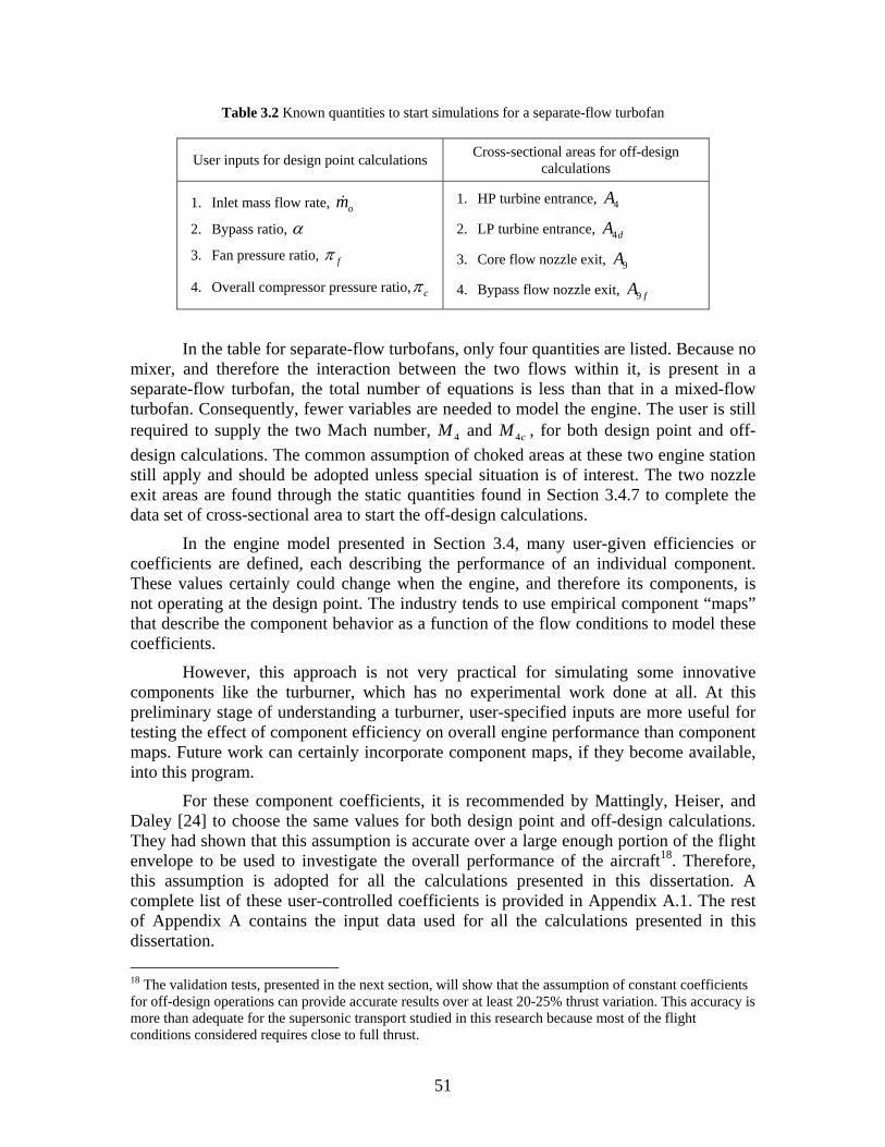
Table 3.2 Known quantities to start simulations for a separate-flow turbofan

User inputs for design point calculations Cross-sectional areas for off-design calculations

1. Inlet mass flow rate, om2. Bypass ratio, α

3. Fan pressure ratio, fπ

4. Overall compressor pressure ratio, cπ

1. HP turbine entrance, 4A

2. LP turbine entrance, 4dA

3. Core flow nozzle exit, 9A

4. Bypass flow nozzle exit, 9 fA

In the table for separate-flow turbofans, only four quantities are listed. Because no mixer, and therefore the interaction between the two flows within it, is present in a separate-flow turbofan, the total number of equations is less than that in a mixed-flow turbofan. Consequently, fewer variables are needed to model the engine. The user is still required to supply the two Mach number, 4M and 4cM , for both design point and off-design calculations. The common assumption of choked areas at these two engine station still apply and should be adopted unless special situation is of interest. The two nozzle exit areas are found through the static quantities found in Section 3.4.7 to complete the data set of cross-sectional area to start the off-design calculations.

In the engine model presented in Section 3.4, many user-given efficiencies or coefficients are defined, each describing the performance of an individual component. These values certainly could change when the engine, and therefore its components, is not operating at the design point. The industry tends to use empirical component “maps” that describe the component behavior as a function of the flow conditions to model these coefficients.

However, this approach is not very practical for simulating some innovative components like the turburner, which has no experimental work done at all. At this preliminary stage of understanding a turburner, user-specified inputs are more useful for testing the effect of component efficiency on overall engine performance than component maps. Future work can certainly incorporate component maps, if they become available, into this program.

For these component coefficients, it is recommended by Mattingly, Heiser, and Daley [24] to choose the same values for both design point and off-design calculations. They had shown that this assumption is accurate over a large enough portion of the flight envelope to be used to investigate the overall performance of the aircraft18. Therefore, this assumption is adopted for all the calculations presented in this dissertation. A complete list of these user-controlled coefficients is provided in Appendix A.1. The rest of Appendix A contains the input data used for all the calculations presented in this dissertation. 18 The validation tests, presented in the next section, will show that the assumption of constant coefficients for off-design operations can provide accurate results over at least 20-25% thrust variation. This accuracy is more than adequate for the supersonic transport studied in this research because most of the flight conditions considered requires close to full thrust.

51

After all the required inputs have been established, the engine model can be run to predict the off-design performances. However, because the known major inputs are at the later stations of the engine, an iterative scheme or a system of equations solver is needed for the entire engine model. Fortunately, MathCAD has a built-in solver for a system of equations, so the program is modified to take advantage of this capability without developing our solution seeking scheme. With the modification completed, the program is put through several tests for validation purpose, as discussed in the next section.

3.6 Validation Tests of the Program

As with any numerical studies or program development, a test to validate the accuracy of the program is in order. Because there is no existing turburner engine, data from current turbofan engines are used to test the accuracy of the program. Since the equations used to describe a turburner is exactly the same as those for a turbine, it is hoped that the accuracy demonstrated in modeling a turbine provides a good indication of the accuracy in modeling a turburner.

As our model requires the user to choose many coefficients, the data of an engine operating at one flight or throttle condition is first used to tune these coefficients to produce the most accurate result at this condition. Other flight or throttle conditions are then calculated based on these coefficients to compare to published data. Consequently, at least two published data points of an engine are needed for this validation test. The choice of engine is really limited as most data published only contains one data point. Fortunately, two engines are found with enough data to perform the test. These data are included in Appendix B and the comparison between these data with the prediction of our model is discussed in this section.

3.6.1 Simulation of a Mixed-flow Turbofan Engine

For the mixed-flow turbofan engine, full and partial throttle data of the General Electric F101-GE-102 engine, powering the B-1B bomber, are found in the book by St. Peter [31]. These experimental data are measured at sea level when engine is static (not moving) and the atmospheric condition is the standard state of 1 atm and 15 °C. A total of three data point is included and the data point for the maximum thrust level is used to tune our program. The program is then throttled down until the lowest thrust level in the published data set is reached. The calculated thrust is then shown in Figure 3.4.

52

0

2000

4000

6000

8000

10000

12000

14000

16000

18000

300 310 320 330 340 350 360

Mass Flow Rate (lbm/s)

Thru

st (l

bf)

Published Data Computed Data Figure 3.4 Comparison between predicted and published thrust of F101 engine

From the figure, one can clearly see that the calculated thrust is slightly lower than the predicted thrust, but the difference is very small. The two trust curves also have smaller differences in the middle, where the mass flow rate is around 340 lbm/s. Considering that all efficiencies are assumed constant for the calculated thrust, this trend is likely to be the result of worse component efficiencies of the actual engine at that range of mass flow and operating conditions.

The results from thrust prediction are certainly encouraging, but another engine performance indicator is also available from the published data in the form as Thrust Specific Fuel Consumption (TSFC). TSFC is defined as the fuel mass flow per unit thrust generated,

fuelmTSFC

F= (3.77)

where fuelm is the overall fuel flow to the engine and F is the thrust generated by the engine. Because this value is a consumption rate, lower values indicate better performance, translating to more fuel efficient engines. Figure 3.5 shows the difference between the published and predicted TSFC for F101.

53

0.000

0.100

0.200

0.300

0.400

0.500

0.600

300 310 320 330 340 350 360

Mass Flow Rate (lbm/s)

TSFC

(lbm

-hr/l

bf)

Published Data Computed Data Figure 3.5 Comparison between predicted and published TSFC of F101 engine

Unlike the predicted thrust data, the predicted TSFC’s are slightly higher than the actual TSFC data published. Combining the facts that the predicted thrust is lower while the TSFC is higher, it is clear that the predicted engine is performing worse than the actual engine. This result is not surprising as the model is tuned at the maximum thrust point, which typically is not the maximum efficiency point, so the assumption of constant efficiencies will certainly leads to worse performances at partial throttle settings that have better actual component efficiencies.

On the other hand, the difference between the two curves is still very small, although the differences between the two TSFC curves shown in the above figure seem to be larger than the differences observed in Figure 3.4. This observation can be more easily explained with the actual values used to generate the two plots, listed in Table 3.3.

Table 3.3 Published and predicted performances of F101 engine

mo Thrust TSFC mo Thrust TSFC Thrust TSFClbm/s lbf lbm/lbf-hr lbm/s lbf lbm/lbf-hr % %

355 17390 0.562 355.0 17213 0.5670 -1.02% 0.89%340 15650 0.540 343.8 15918 0.5604 -1.10% 3.33%313 13030 0.523 332.9 14691 0.5541 -3.25% 4.16%

322.1 13525 0.5486311.0 12415 0.5440

Published Data Computed Data DifferenceF101-GE-102

One can clearly see from the table that the mass flow rates of actual and calculated data are different, except the maximum thrust point where the program is tuned. The difference is caused by the fact that throttle setting is controlled by engine temperature rather than inlet mass flow rate in this program, so an exact match between the mass flow rates will require several iterations. To compare the two data sets, 2nd-order curve fits are generated from the predicted data to express the thrust and TSFC as

54

functions of mass flow rate. Then, the thrust and TSFC corresponding to the mass flow rates in the published data are generated and compared.

From the percentage differences in the right most columns, the two data sets have the best match at the maximum thrust point where the computational model is tuned. The differences grow as the operating point moves away from the maximum thrust point, but no more than 5% difference is recorded in the available range of actual data. Again, because of the lack of more data, it is hard to provide statistically meaningful projection about the growth of error as the throttle setting is lowered further.

Overall, the predicted performances are lower than the actual data, even at the maximum thrust point (suggesting more tuning may be needed), but the error is small and the results are fairly accurate. From this test, we can conclude that the program is producing accurate results both at the design point and over a range of off-design conditions for a mixed-flow turbofan.

3.6.2 Simulation of a Separate-flow Turbofan Engine

Also in the same book by St. Peter [31] is a set of experimental data for General Electric TF34-GE-100 engine (see Appendix B). TF34 is a separate-flow turbofan engine used in a wide variety of business jets as well as the A-10A of US Air Force. Because a module for separate exhausts is included in this program for potential future supersonic business jets, the published data provide a good test opportunity to demonstrate the program is performing as expected and is ready for future uses to study on the particular application.

For the published data, the same set of standard conditions listed in the previous section is used when measuring the performance of TF34. For the computational model, the maximum thrust point is again used as the tuning point for all component coefficients and efficiencies. The published data and calculated results are listed in Table 3.4.

Table 3.4 Published and predicted performances of TF34 engine

mo Thrust TSFC mo Thrust TSFC Thrust TSFClbm/s lbf lbm/lbf-hr lbm/s lbf lbm/lbf-hr % %

333 9065 0.371 333.0 9066 0.3712 0.01% 0.05%314 7990 0.369 318.1 8301 0.3804 0.89% 2.23%301 7335 0.355 313.5 8048 0.3794 0.76% 6.57%

304.3 7554 0.3778299.6 7312 0.3771

Published Data Computed Data DifferenceTF34-GE-100

Similar method to the one described in the previous section is used to resolve the different numbers of data points between the two data sets. Clearly, the thrust prediction is extremely accurate, with less than 1% error for the range of published data. This accuracy is also reflected in Figure 3.6, where two data lines are so close to each other that it is hard to distinguish between them.

55

0

1000

2000

3000

4000

5000

6000

7000

8000

9000

10000

290 300 310 320 330 340

Mass Flow Rate (lbm/s)

Thru

st (l

bf)

Published Data Computed Data Figure 3.6 Comparison between predicted and published thrust of TF34 engine

On the other hand, the TSFC errors in Table 3.4 increases more rapidly and actually reaches a 6.57% difference at the point with lowest published thrust value. When the two data sets are plotted, as shown in Figure 3.7, it could be seen that the curvature of the curve formed by actual data points is very pronounced when compared to the predicted performance line. As a result, the left most point has a much larger error while the range in the middle (about 310-330 lbm/s) actually has a smaller error. In fact, when compared to the errors in simulating the mixed-flow turbofan presented earlier, the percent TSFC errors are less than those of the mixed-flow turbofan in most of the mass flow rates calculated.

0.000

0.050

0.100

0.150

0.200

0.250

0.300

0.350

0.400

290 300 310 320 330 340

Mass Flow Rate (lbm/s)

TSFC

(lbm

-hr/l

bf)

Published Data Computed Data Figure 3.7 Comparison between predicted and published TSFC of TF34 engine

From these results, the accuracy of the program when simulating a separate-flow turbofan is demonstrated. The thrust level in the range calculated is consistently within

56

1% difference of the actual data and the TSFC error is also small. The error does vary somewhat, as expected, because of the assumption of constant efficiencies, but overall it is small enough for users to use this program with great confidence.

While the difference in curvature of the two TSFC data set results in a larger error when the engine is throttled down, it should be keep in mind that the number of actual data points is at the minimum needed to generate a 2nd-order curve-fit. The uncertainty associated with extrapolation from the curve-fit of actual data will be significant and most likely will outweigh the difference between the model prediction and the curve-fit of actual data. Therefore, even though increased error is expected as operating conditions vary, how fast the error increase with respect to the change of operating conditions can not be concluded from the few data points.

3.7 Summary

In conclusion of this chapter, a cycle analysis program is created for this research, based on a twin-spool, mixed-flow turbofan with possible introduction of ITB and turburners. The baseline turbofan is the current choice for propelling supersonic aircraft, while older generation twin-spool turbojet engines that had propelled supersonic aircraft can be simulated by enforcing a zero bypass ratio19. In addition, a single-spool engine can be approximated by using an ideal fan and an ideal turbine of unity compression ratio. A separate-flow module is also created for future investigations of different engine configurations satisfying other needs.

As far as the combustion is concerned, there are five possible places for combustion, including the afterburner and each burner can be used independent of other burners. The program cannot model every current aircraft engine at this stage, but it is sufficient for current study of a turburner engine and it is modular enough for future expansion or modification. The gases used in the program are assumed to be gaseous mixtures of four species in chemical equilibrium. The individual species are assumed to be thermally perfect gases, so the mixture also behaves as a thermally perfect gas.

The actual engine model is made of seven major modules, some used more than once to represent similar components. All the assumptions and procedures used to create these modules are discussed in great details to show the strength and room for improvement or growth of the engine model. The model is also modified to calculate the off-design performance of an engine by assuming some cross-sectional areas are constant in off-design conditions. In addition, several Mach numbers and most user-given coefficients are also assumed to remain constant in off-design conditions to close the system of equations.

Finally, tests to demonstrate the accuracy of the newly developed program are presented. The results show that the program is very accurate and is ready to use. Granted, there is no experimental data on a turburner engine to test the accuracy of the turburner model, but this deficiency is true to any work that intends to predict the performance of an innovative cycle. Because the turburner model is exactly the same as

19 To speed up calculations, a dedicated turbojet solver for off-design calculations is still created.

57

the turbine model, it is believed that the accuracy demonstrated in modeling a turbine provides good indication of the accuracy in modeling a turburner. If any future numerical or experimental work shows that the model used in this program to be less than satisfactory for the turburner, this program is also designed to accommodate quick modifications and re-calculations to improve accuracy.

58

Chapter 4 Results and Discussions

As stated in previous chapter, the goal of this research is to identify the benefit of using a turburner engine in a realistic environment, taking into consideration the details of parameters that have not been modeled before but are known to have great impact on the performance. Different engine configurations and design parameters should be examined to find an optimum design (or range of designs) for a turburner engine, which could allow for more focused research on how to produce such an engine. Ultimately, it is hoped that a turburner engine will show significant improvement in the interested application – a supersonic cruising aircraft for commercial, military, or space purpose – and therefore moves forward the research into turburner technology as well as next generation of supersonic aircraft.

In order to perform the required task, the computer program described in Chapter 3 was developed to simulate a turburner engine. The program has been shown to offer great accuracy, so the next step is to use the program and calculate the performance of a turburner engine. However, designing an engine involves substantial amount of compromises between the conflicting requirement and an optimum design for one requirement may be the worst design for another requirement. With the advances in computer technology, current practice to address the complicated designing phase is to use multi-disciplinary design optimization where different programs for the systems in an aircraft are linked together and solved simultaneously to find the best solution.

It is indeed hoped (and care has been taken to ensure) that the program developed in this research can be used in the future in a multi-disciplinary design optimization. However, it is beyond the scope of this research to perform such optimization – or to build all the components necessary to do so. Instead, a particular application is picked first, followed immediately by preliminary calculations to eliminate several configurations of the engine. Finally, extreme cases where all parameters are chosen to maximize only one performance of the engine are studied. While the results shown are most likely local optima rather than global optima, the data should be enough to demonstrate the superiority of a turburner engine.

In this chapter, the explanations and results of these calculations are presented. An application in the form of a next generation supersonic transport is chosen to establish the requirement for engines. Constraints based on current level of engine technology are also added and discussed to form the complete requirement for engines. Results from preliminary design point calculations are presented next; these results are used to choose the most promising configuration. Once the configuration is chosen, the amount of turbine cooling, based on experiences with current turbines, is calculated and discussed. Two requirements, aircraft range and engine size, are then chosen to be optimized and used to highlight the strength of a turburner engine in a supersonic aircraft. The case with maximizing the range of the aircraft is examined first, followed by the case of minimizing the size of the engine. A special discussion regarding cooling, based on the

59

observations on the results, is presented next. Finally, a summary of findings is used to conclude this chapter.

4.1 Mission Requirement and Operation Limit of the Engine

Because the interest of this research is to identify the benefits of using a turburner engine on a supersonic aircraft, the mission requirements can be set by examining current supersonic aircraft and their engines. As mentioned earlier, the Concorde and the Blackbird are the two aircraft that were designed to cruise supersonically. Data and information for the Blackbird are still scarce in the public domain because of its classified missions, but many studies on the Concorde and its potential replacement are available.

In this research, the study on a next generation supersonic transport done by Lowrie et al. [32] is used as a guideline to set up a mission requirement. In addition, the excellent work by Rech and Leyman [33] on the difficulties experienced and solutions found during the development of Concorde is used as supplemental information. Other sources are used when some updated information are needed regarding current level of technology.

Using the above information, a summary of the characteristics of the aircraft is listed below:

1. The maximum take-off weight (MTOW) of the aircraft is 500,000 lb, 25% heavier than the Concorde, to satisfy the increased requirement in range and payload.

2. The aircraft is propelled by four engines.

3. The aircraft is to cruise at Mach 2.0 and at the altitude of 60,000 ft. The cruise speed is the same as Concorde because no special skin treatment to the aircraft is needed to counter the frictional heat and thermal stress due to flight speed. On the other hand, the cruise altitude is set higher than the normal cruise altitude of Concorde, 53,000 ft, to avoid conflicting with other subsonic aircraft that are flying at higher altitudes20.

4. The aircraft must achieve a range of 5,700 nautical miles with a fuel fraction (see explanation after the list) of 0.4 to remain commercially competitive. These requirements are equivalent to a required TSFC of 1.0306 lb/hr-lbf (pound per hour per pound force) at cruise condition for each engine.

5. Life-to-drag ratios of the aircraft in four critical flight conditions are assumed based on the potential progress in airframe aerodynamics. These ratios are used to determine the thrust requirement of the engines.

These requirements for the aircraft certainly translate to a set of requirements for the engine. However, it is worthwhile to briefly describe the lift-to-drag ratio and fuel fraction for readers not familiar with aircraft design before discussing their implications on the engine requirements. 20 Because the airspace is more saturated today, more and more subsonic aircraft are flying at higher altitudes. In fact, some newer subsonic aircraft are even designed with optimum cruise altitude at about 50,000 ft.

60

As mentioned earlier, lift-to-drag ratios are needed to determine the thrust requirement of the engine. Lift-to-drag ratio is an indicator of aerodynamic performance defined (simply) as

LLD D

= (4.1)

where L is the lift force and D is the drag force. When aircraft is flying at a constant speed, the lift force is balanced with the weight of the aircraft and the drag force equals to the thrust. Once the lift-to-drag ratio is known, the thrust required to maintain level flight with constant speed can be found with the ratio and the weight of the aircraft by evoking the relationship

L L

D D

L WThrust D= = = (4.2)

Of course, if the aircraft is accelerating, the thrust requirement is increased to satisfy the desired acceleration.

Based on the guideline suggested by Lowrie et al., four flight conditions are considered critical in ensuring the success of the aircraft in this research. The lift-to-drag ratios for the four conditions are chosen, based on the projected progress in airframe design. The accelerations of the aircraft are also chosen for some conditions and the engines must provide the required thrust and fuel consumption at all four conditions. Table 4.1 summarizes the four flight conditions and their corresponding lift-to-drag ratio, required acceleration, and required thrust.

Table 4.1 Information on the four critical flight conditions

Condition Number (ft) L/DMach Altitude Acceleration (G, 1 G = 9.81 m/s2)

Thrust (lbf)

Take-off 0.30 0 5 0.2 50000Subsonic Cruise 0.95 36000 15 0.0 8500Transonic Acceleration 1.20 40000 10 0.1 25000Supersonic Cruise 2.00 60000 10 0.0 12500

From the table, one can see that the lift-to-drag ratio is lowest at take-off and highest at the subsonic cruise point. Once the flight speed increases pass Mach 1, the lift-to-drag ratio is lowered again as the wave drag, caused by shocks, starts to increase the drag force substantially. However, as the speed becomes closer to the design point, the lift force is able to balance with the drag force with a lift-to-drag ratio that is the same as in transonic acceleration. Overall, the lift-to-drag ratios are higher than those of Concorde, but the values are deemed achievable based on the survey done by Lowrie et al. For example, the lift-to-drag ratios of the Concorde are 8 and 13 for the supersonic and subsonic cruise points, respectively. On the other hand, 10 and 15 are assumed in this research for the two cruise conditions.

When the aircraft is cruising supersonically, the balance between forces leads to a 50,000 lbf thrust requirement for the four engines combined. As a result, each engine

61

must produce 12,500 lbf of thrust, which is the value shown in the right most column of the table.

Before the aircraft actually reaches the supersonic cruise point, another critical condition is the transonic acceleration phase where extra thrust is needed to provide the acceleration and sometimes climbing of the aircraft. Only level acceleration is considered in this research and the value chosen is 0.1 G, the common value chosen to avoid passenger discomfort. As a result of the acceleration requirement, the thrust requirement is doubled to 25,000 lbf when compared to the supersonic cruise point, even though the lift-to-drag ratio is the same for both cases.

Although the aircraft to design to cruise supersonically, current regulations still restrict supersonic over-fly above inhabited areas. Consequently, a subsonic cruise requirement is also set to ensure the aircraft can operate at this condition efficiently for long period of time if called for. At this point, the thrust requirement is the lowest as the lift-to-drag ratio is the highest. Therefore, it is not expected that any engine satisfying the other requirements will have trouble meeting the thrust requirement at this point. However, the TSFC when the engine is throttled down to meet the required thrust is examined to determine which engine provides the best fuel economy.

During the take-off, the lift-to-drag ratio is the lowest because the low dynamic pressure coming to the wings and because the wings are not operating at the speed range that they are designed for. Worse, to ensure a safe take-off if one engine failed, 0.2 G acceleration for the combined thrust of four engines is required. If an engine fails, 0.1 G acceleration can still be maintained by the remaining three engines. As a result, the thrust required for each engine is the highest at 50,000 lbf.

It should be noted that even though the thrust at take-off is four times of that at supersonic cruise, the supersonic cruise is still the most demanding thrust requirement in this research because the amount of mass flow available from the dense air at sea level is much greater than the thin air at 60,000 ft. On the other hand, either transonic acceleration or take-off could easily become the most demanding case if the assumptions about the lift-to-drag ratio and the required acceleration are changed. A vivid example is that the Concorde only used afterburning during take-off and transonic acceleration, not at the cruise condition.

Once the thrust requirements for the engine have been established, the requirement for fuel consumptions is examined. To understand the relationship between the aircraft range and engine fuel consumption, the term “fuel fraction” must be explained first. The fuel fraction is the fraction of the fuel weight to the gross aircraft weight,

fuel fuel

gross structure payload fuel

W WW W W W

=+ +

(4.3)

Clearly, a larger fuel fraction will translate to longer range as more fuel is carried. However, for a given gross aircraft weight, higher fuel fraction means less payload – unless material technology improves and reduces the weight of the structures. Therefore, for a commercial airliner, it is desired to reduce the fuel fraction to make room for the payload while maintaining the range of the aircraft.

62

Based on surveys of routes and experiences with operating cost, Lowrie et al. established that a next generation supersonic transport can only be commercially viable if it can achieve 5,500 nautical miles with a fuel fraction less than 0.4. As the survey is somewhat dated and newer routes may have materialized recently, a more stringent range requirement of 5,700 nautical miles is set in this research.

The required range and fuel fraction of the aircraft certainly translate to a requirement of fuel consumption for the engines. The requirement for the engines can be found by using the Brequet range equation,

ln gross

gross fuel

WL VRangeD TSFC W W

⎛ ⎞= ⋅ ⋅ ⎜⎜ −⎝ ⎠

⎟⎟ (4.4)

where L is the lift force, D is the drag force, V is the flight speed, and TSFC is the thrust specific fuel consumption defined in Equation (3.77). Equation (4.4) can also be expressed in terms of fuel fraction as

1ln1 fuel

gross

WW

L VRangeD TSFC

⎛ ⎞= ⋅ ⋅ ⎜⎜ −⎝ ⎠

⎟⎟ (4.5)

Then, using a flight speed, V, of 1,150 knot (equivalent to the speed of Mach 2 at 60,000 ft), the cruise lift-to-drag ratio of 10, and a fuel fraction of 0.4, we find that TSFC must be less than or equal to 1.0306 lb/hr-lbf to satisfy the required range of 5,700 nautical miles.

In addition to requirements stem from the mission needs of the aircraft, the engine is also subject to limitations of current engine technology. Because the fatigue life of the material deteriorates greatly with operating temperature, engine components cannot operate beyond certain temperatures. The needs to supply relatively cold air for cooling the turbine also impose a temperature limitation on the air at the exit of the compressor. Therefore, several limits on component temperature are imposed based on current technology. These limits are summarized in the list below:

1. The highest allowable temperature in the engine is 3,240 R (1,800 K) except in the afterburner. In an engine, the most likely location to have temperature close to this limit is the high-pressure turbine inlet temperature, , immediately after the main combustor. However, if a high-pressure turburner or a Interstage Turbine Burner (ITB) is used, the exit temperature of the high-pressure turburner, , and the low-pressure turbine inlet temperature, , must also be compared against this limitation.

4tT

4bT

4cT

2. It is also assumed that the components cannot operate in the maximum allowable temperature, 3,240 R, for an extended amount of time, so the allowable temperature is lowered to 3,078 R (1,710 K or 95% of the maximum allowable temperature) at both subsonic and supersonic cruise conditions.

3. The highest temperature allowed in an afterburner is 3,960 R (2,200 K). The afterburner can only be used in transient flight conditions, such as transonic acceleration or take-off, for acceptable fuel consumption rate.

63

4. The compressor discharge temperature, , must be less than or equal to 1,800 R (1,000 K) to provide sufficient cooling to the turbines.

3tT

The values for the above limitations are chosen based on the suggestion by Mattingly et al. [24] and Walsh and Fletcher [28]. Several component temperatures have actually been demonstrated in real engines [2], so the limits chosen should represent current level of technology fairly well.

With the limits on engine components set, the definition of engine requirements for this research is completed. The engine must produce sufficient thrust while maintaining low fuel consumption in several critical flight conditions for the desired supersonic transport. On the other hand, the engine must also be able to be manufactured with the current level of technology. A closer examination of all the requirements reveals that the supersonic cruise point presents the greatest challenge in the four flight conditions chosen. Consequently, the engine should be designed to produce optimum performance at this flight conditions and the supersonic cruise condition is chosen as the design point.

With the design point chosen and requirements of the engine identified, the next step is to choose the parameters of an engine to satisfy the requirements. However, the program developed in this research allows for several different engine configurations. For example, a turburner can replace either the high-pressure turbine or the low-pressure turbine, or both. Therefore, the performances of different configurations at the design point must be examined first to determine the most promising configuration. The discussions on these different configurations are presented next.

4.2 Preliminary Examination of Possible Engine Configurations

When a design point is chosen, typically the parametric performance at this point is examined first. By varying different engine parameters, such as bypass ratio, designers choose several combinations of engine parameters as preliminary designs. Then, these designs are sized21 and the off-design performances of these designs are calculated to find the optimum design for the mission.

However, for this research, additional calculations are needed because the program not only allows for variations in engine parameters, but also includes several engine cycles that produce potential improvement in performance. Therefore, preliminary calculations that not only vary the engine parameters, but also vary the engine configurations to accommodate different engine cycles are needed. From these calculations, the most promising engine configuration is chosen to investigate its performance improvement over a regular turbofan.

As mentioned earlier, the program developed in this research allows several different ways to incorporate turburners into an engine. In fact, the program also includes model to study the Interstage Turbine Burner (ITB). To understand the different engine 21 Most cycle analyses are carried out in a zero-dimensional way by normalizing against engine mass flow rate. When the designs are “sized”, the mass flow rate is chosen so the actual thrust of the engine can be calculated.

64

configurations discussed in this section, one must first recall the structure of the program, shown in Figure 3.1 and repeated here as Figure 4.1.

5f

Figure 4.1 Schematics of a twin-spool, mixed-flow turbofan engine model

In the figure, one can see that there are five components that combustion can occur within: the main combustor (MB), the high-pressure turburner (HPTB), the Interstage Turbine Burner (ITB), the low-pressure turburner (LPTB), and the afterburner (AB). Clearly, several configurations can be created by combining different combustors in an engine. For example, an engine can be designed with a main combustor and an ITB between regular high-pressure and low-pressure turbines, while another can be designed with an HPTB in addition to the main combustor, while retaining a regular low-pressure turbine.

1 2 33f 3a0 4 54a 4b 4c 4d 6 7 8 9

Q Q Q Q Q

bleed air

fan & low pressure

compressor

high pressure

compressor

main combustor

HPT coolant mixer

high pressure turbine

interstage turbine burner

LPT coolant mixer

low pressure turbine

HPT coolant

LPT coolant high-speed spool

low-speed spool

Reference Stations: Abbreviations:0 Free stream LPC Low-pressure compressor 1 Inlet or diffuser entry HPC High-pressure compressor 2 Fan or LPC entry MB Main combustor 3f HPC entry HPT High-pressure turbine 3 HPC exit HPTB High-pressure turburner 3a MB entry ITB Interstage turbine burner 4 MB exit LPT Low-pressure turbine

HPT/HPTB coolant mixer entry LPTB Low-pressure turburner 4a HPT/HPTB coolant mixer exit AB Afterburner

HPT/HPTB entry C-D Convergent-divergent 4b HPT/HPTB exit

ITB entry 4c ITB exit

LPT/LPTB coolant mixer entry 4d LPT/LPTB coolant mixer exit

LPT/LPTB entry 5 LPT/LPTB exit

Core stream mixer entry 5f Bypass stream mixer entry 6 Mixer exit

AB entry 7 AB exit

C-D nozzle entry 8 C-D nozzle throat 9 C-D nozzle exit

65

As discussed in the previous section, the supersonic cruise point is chosen as the design point for the engine because the requirement at this flight condition is the most challenging and it is expected that an engine satisfying the requirement at this flight condition should have no difficulty in meeting the requirement at other flight conditions. Therefore, the design point performances of different engine configurations are used to choose the most promising configuration to provide significant improvement over a regular turbofan engine.

To choose the engine configurations to be studied in the preliminary calculations, the requirement of the engine established in the previous section is used. Because the requirement states that the afterburner cannot be used during the supersonic cruise, it is eliminated from the engine configurations considered in this section. Note that this assumption does not mean that any of the engine configurations presented do not or can not have an afterburner. Also, the main combustor is assumed to be present and always on, as the limitation on compressor discharge temperature prohibits the use of the Ramohalli cycle.

With these considerations and constraints, five different cases are set to exploit the performance benefit brought by different combinations of the five potential combustors mentioned above. These five cases are:

1. Baseline case with only a main combustor.

2. Only an HPTB is present in addition to the main combustor.

3. Only a LPTB is present in addition to the main combustor.

4. Both HPTB and LPTB are present in addition to the main combustor.

5. Only an ITB is present in addition to the main combustor.

Once the configurations to be examined are chosen, engine parameters are selected to begin the calculations. A complete list of these parameters can be found in Appendix A.3. For ease of discussion, some key parameters are presented briefly here. All calculations assume an overall compressor pressure ratio, cπ , of 20 at the supersonic cruise condition to satisfy the limit on compressor discharge temperature. Other temperature limits set in the previous section are also followed. In addition, two bypass ratios (BPR), one and five, are examined to determine how the performance of each configuration varies with the bypass ratio.

In the calculations presented in this section, the amount of turbine cooling for all configurations is assumed to be the same as the amount used in the baseline turbofan configuration (calculations presented in the next section, Section 4.3). While this assumption is not accurate in itself, the differences in the calculated performances between each configuration are very substantial. Consequently, the inaccuracy in the assumption is not expected to outweigh the differences and change the conclusion. A further examination of the sensitivity of engine performance to the amount of cooling also reveals that the cooling in a turburner do not affect the performance as much as the cooling in a turbine (this discussion is presented in Section 4.6). As a result, no further calculations using different amounts of turbine cooling flow are carried.

66

With the parameters chosen, the first case to be examined is when bypass ratio is one. It is common knowledge that the optimum bypass ratio at the design point of a turbofan engine decreases as the flight speed increases. On the other hand, a higher bypass ratio is desired for better fuel economy. As a result, a bypass ratio of one represents a low bypass ratio that should provide good performance in supersonic speed. Figure 4.2 shows the design specific thrusts of the five configurations.

20

25

30

35

40

45

50

55

60

65

70

1.50 2.00 2.50 3.00 3.50 4.00 4.50 5.00 5.50 6.00

Fan Pressure Ratio

Spec

ific

Thru

st (l

bf-s

/lbm

)

Turbofan HPTB LPTB HPTB & LPTB ITB Figure 4.2 Specific thrust at supersonic cruise (BPR = 1)

In the figure, one will notice that the specific thrust actually varies with the fan pressure ratio and the optimum fan pressure ratio for maximum specific thrust is quite different from one configuration to another. In fact, the range of acceptable fan pressure ratio is also different between configurations because the pressure differences between the fan and the core streams can not be too large in order to satisfy the Kutta condition enforced at the inlet of the mixer.

From Figure 4.2, it is quite clear that having both HPTB and LPTB provides the most increase in specific thrust, with more than 100% increase over the baseline case. Using either an HPTB or an ITB, each with 60%~70% increase, presents the next best option to increase the specific thrust. Using only the LPTB, the specific thrust varies greatly with the fan pressure ratio chosen and reaches a maximum at the largest fan pressure ratio acceptable. On the other hand, the LPTB option could still provide about 45% improvement over the turbofan with the largest fan pressure ratio acceptable.

Obviously, all four configurations with additional combustion inside turbine provide significant improvement in the specific thrust over a regular turbofan. For applications where thrust is needed in high speed, these four configurations are certainly much more promising than the traditional turbofan. However, because all four configurations use additional combustion, the additional fuel flow used must also be evaluated to determine the cost of such drastic improvement in specific thrust. This comparison of TSFC between all configurations is shown in Figure 4.3.

67

1.00

1.05

1.10

1.15

1.20

1.25

1.30

1.35

1.40

1.50 2.00 2.50 3.00 3.50 4.00 4.50 5.00 5.50 6.00

Fan Pressure Ratio

Thru

st S

peci

fic F

uel C

onsu

mpt

ion

(lbm

/hr-

lbf)

Turbofan HPTB LPTB HPTB & LPTB ITB Figure 4.3 TSFC at supersonic cruise (BPR = 1)

In the above figure, it is immediately apparent that the ITB configuration requires much more additional fuel than any other configurations. Using both an HPTB and a LPTB consumes more fuel than using either one of them separately, as expected, but it is interesting to see that using HPTB alone is actually the most fuel efficient among the four configurations with combustion within the turbine. In fact, almost no additional fuel is required for the HPTB configuration, as evidenced in Table 4.2.

Table 4.2 Performance comparison between different configurations (BPR = 1)

Specific Specific Fan Thrust TSFC Thrust TSFC

lbf-s/lbm lbm/hr-lbfTurbofan 2.00 31.3881 1.0548 100.00% 100.00%HPTB 3.50 50.0172 1.0609 159.35% 100.59% 10113.13%LPTB 2.25 39.9737 1.0924 127.35% 103.57% 767.10%HPTB & LPTB 4.00 64.4660 1.1239 205.38% 106.56% 1606.96%ITB 3.50 50.9173 1.1923 162.22% 113.04% 477.27%

Configurationnormalized vs. turbofan

Specific Thrust increase per TSFC increasePressure

Ratio

In Table 4.2, the fan pressure ratio that produces the best TSFC is chosen as the optimum fan pressure ratio because fuel consumption is of the greatest concern in the cruise condition. Observations made earlier regarding Figure 4.2 and Figure 4.3 can also be seen in the performance values normalized against the turbofan performance shown in the columns in the center of the table. Because it is desired to maintain low TSFC while achieving high specific thrust, these normalized values are used to create the data in the right most column, where the percent increase in specific thrust is divided by the percent increase in TSFC. The data created could be roughly considered as a cost-effectiveness indicator of using the configuration, where higher values indicate better performance improvement with the same amount of additional TSFC.

68

Clearly, the HPTB configuration is the best choice in the situation considered, using a 0.59% increase in TSFC to achieve the 59% increase in specific thrust. In fact, looking at the data in the right most column, the cost-effectiveness indicator for the HPTB is at least a order-of-magnitude larger than any other configurations. As a result, it is unlikely that any inaccuracy caused by the assumptions made for these calculations, such as the assumption about turbine cooling flow, would change the result that HPTB is the best configuration for the conditions given.

On the other hand, a closer examination of the TSFC values reveals that none of the configurations meet the needed TSFC of 1.0306 lb/hr-lbf to satisfy the range requirement. Consequently, the bypass ratio of each configuration must be increased to lower TSFC and achieve the required range.

To investigate the change in performance when the design bypass ratio is varied, a somewhat extreme case of bypass ratio equal to five is used. In this case, the fuel economy should be better than the requirement but the specific thrust may be low and the resulting engine may be too large. It is expected that the bypass ratio chosen for the final design will be between the two values, one and five, chosen here. Therefore, the best configuration for the two boundary values should also be the best configuration within the range enclosed by the two values. The specific thrusts for engines with bypass ratio of five are shown in Figure 4.4.

5

10

15

20

25

30

35

1.15 1.35 1.55 1.75 1.95 2.15 2.35 2.55 2.75

Fan Pressure Ratio

Spec

ific

Thru

st (l

bf-s

/lbm

)

Turbofan HPTB LPTB HPTB & LPTB ITB Figure 4.4 Specific thrust at supersonic cruise (BPR = 5)

In Figure 4.4, using both HPTB and LPTB again provides the best specific thrust, followed by using either an HPTB or an ITB. Using LPTB and the traditional turbofan still provide the least specific thrust. Worth noting is the fact that the HPTB and the ITB configurations now produce almost exactly the same specific thrust, the only difference is in their respective fan pressure ratio that produces the maximum specific thrust.

69

Another interesting fact is that using both HPTB and LPTB provides almost three times the specific thrust of a traditional turbofan while using either an HPTB or an ITB produces twice the specific thrust of a regular turbofan. This finding clearly indicates that, when compared to regular turbofan, introducing any additional combustion within turbines can reduce the decrease in specific thrust as a result of increasing bypass ratio. If the TSFC is also lowered through the increase of bypass ratio, a supersonic engine with better fuel economy than any current engine, yet produces the same amount of thrust, can be made possible. Interestingly, the TSFC does not always decrease with the increase of bypass ratio in the situation studied, as evidenced in Figure 4.5.

0.80

0.85

0.90

0.95

1.00

1.05

1.10

1.15

1.20

1.25

1.30

1.15 1.35 1.55 1.75 1.95 2.15 2.35 2.55 2.75

Fan Pressure Ratio

Thru

st S

peci

fic F

uel C

onsu

mpt

ion

(lbm

/hr-

lbf)

Turbofan HPTB LPTB HPTB & LPTB ITB Figure 4.5 TSFC at supersonic cruise (BPR = 5)

Surprisingly, the lowest TSFC is achieved by using HPTB rather than a traditional turbofan. In fact, the TSFC of a regular turbofan is only lower than that of the ITB configuration, losing out to the other two configurations using turburners also, as shown in Table 4.3. The results may sound counter-intuitive initially, as using turburners requires additional fuel flow into the turbine and the total amount of fuel used in any configuration with turburner is surely higher than a regular turbofan. On the other hand, one must realize that TSFC is a normalized fuel flow,

fuelmTSFC

F=

so the value of TSFC could remain low even when the fuel flow is high, as long as the generated thrust is even higher. The fact that a turbofan has a higher TSFC does not means it consumes more fuel than any turburner engine, but means that the fuel consumed is not used efficiently and the generated thrust is extremely low.

70

Table 4.3 Performance comparison between different configurations (BPR = 5)

Specific Specific Fan Thrust TSFC Thrust TSFC

lbf-s/lbm lbm/hr-lbfTurbofan 1.35 10.5502 1.0476 100.00% 100.00%HPTB 1.80 20.5008 0.9491 194.32% 90.60%LPTB 1.45 14.9551 1.0391 141.75% 99.19%HPTB & LPTB 2.15 29.8347 0.9815 282.79% 93.70%ITB 1.55 20.5531 1.0893 194.81% 103.98%

Configuration Pressure Ratio normalized vs. turbofan

In Table 4.3, the lowest TSFC produced by each configuration is compared. As mentioned earlier, the specific thrust difference between the turbofan and the other configurations are more substantial, while the three configurations using turburner all produce lower TSFC than the turbofan. Unlike the situation with bypass ratio of one where the HPTB configuration is the clear winner, both the HPTB configuration and the configuration with both HPTB and LPTB show great potential in this case. Further examinations on the two configurations are necessary before one can be chosen for further calculations.

One would also notice that only these two configurations actually meet the TSFC requirement of 1.0306 lb/hr-lbf. While the values certainly show the potential of the two configurations, the extreme change in bypass ratio means that there may still be an optimum point that produces an acceptable combination of specific thrust and TSFC for the other three configurations between the two extreme bypass ratios chosen.

On the other hand, the superiority of a turburner engine for higher bypass ratios is quite interesting. As stated previously, it is a known fact that the optimum bypass ratio for a turbofan decreases as the flight speed increases. The results in Figure 4.5 and Table 4.3 clearly reflect this fact, as the large bypass ratio lowers the specific thrust of a turbofan so much that a penalty is incurred on TSFC. On the other hand, the decrease in specific thrust in a turburner engine is definitely less than a turbofan engine, as the TSFC of any configuration using turburners is lower than that in a turbofan. This fact can be shown more clearly with Table 4.4, where the actual and percent changes in performance between the two bypass ratios are shown.

Table 4.4 Performance variations caused by change in bypass ratio

Specific Thrust TSFC Specific

Thrust TSFC

lbf-s/lbm lbm/hr-lbf lbf-s/lbm lbm/hr-lbfTurbofan 2.00 31.3881 1.0548 1.35 10.5502 1.0476 -66.39% -0.68%HPTB 3.50 50.0172 1.0609 1.80 20.5008 0.9491 -59.01% -10.54%LPTB 2.25 39.9737 1.0924 1.45 14.9551 1.0391 -62.59% -4.87%HPTB & LPTB 4.00 64.4660 1.1239 2.15 29.8347 0.9815 -53.72% -12.67%ITB 3.50 50.9173 1.1923 1.55 20.5531 1.0893 -59.63% -8.64%

Configuration

% change from BPR=1

Specific Thrust TSFCFan

Pressure Ratio

Fan Pressure

Ratio

By-Pass Ratio = 1 By-Pass Ratio = 5

In Table 4.4, the percent change in performance as the bypass ratio increased from one to five is shown in the right most columns. It is interesting to note that the configuration with both an HPTB and a LPTB is able to lose the least amount of specific thrust while reducing the most TSFC, followed by the configuration with an HPTB. In

71

fact, the specific thrust produced by the configuration with both HPTB and LPTB is almost the same as the specific thrust produced by the regular turbofan, yet the TSFC for this configuration is much lower than that of the regular turbofan.

While there may be points between the two bypass ratios that produces even lower TSFC, it is quite clear from Table 4.4 that introducing combustion in the turbine reduces the decrease of specific thrust with respect to the increase of bypass ratio. The reason for this behavior is most likely because the fact that the additional combustion in the high-pressure turbine, or in ITB between high-pressure and low-pressure turbines, is able to energize the flow before it enters the low-pressure turbine. Because of the energized flow and its higher total temperature at the entrance, less total pressure reduction in the low-pressure turbine, which is driving the fan, can be achieved. Consequently, the loss in thrust is less. This reasoning is certainly reinforced by the fact that the worst performer among the four configurations with additional combustion is the LPTB only configuration, the only configuration that has a low total temperature at the entrance to the low-pressure turbine, similar to a regular turbofan.

From Table 4.3 and Table 4.4, one can also say that the optimum bypass ratio of a turburner engine, or an ITB engine, is higher than a turbofan engine. The reason is the same as the argument made in the previous paragraph. Because the flow entering the LPT is more energized and less pressure reduction occurs in LPT, the LPT has more capability to drive a larger fan while still maintaining the thrust. As a result, the optimum bypass ratio for turburner engines is higher than turbofan engines. This higher optimum bypass ratio can ensure the turburner engines produce better fuel efficiency than a turbofan.

From the above results, it is clear that the HPTB configuration is the most promising choice if the bypass ratio is small or close to one. On the other hand, if the bypass ratio is large, there are still two configurations to consider. The HPTB configuration offers better fuel efficiency at the point tested, while the other configuration with both HPTB and LPTB seems to have advantages on specific thrust or when bypass ratio is increased further. The two configurations are the best candidates to introduce engines with relatively high bypass ratio into the design of a fuel-efficient supersonic aircraft.

After some consideration, the HPTB configuration is chosen for further analysis. One reason for this choice is that the application of interest is a supersonic transport, so fuel economy is the primary concern. The HPTB configuration uses the fuel more efficiently than any other configuration, whether the bypass ratio is small or large. Considering that the two bypass ratios studied here are used as the boundary points to define the range of bypass ratios for further calculations, the HPTB configuration should provide better performance within this range. In fact, it is expected that the bypass ratio of the chosen engine would be small, most likely in the range of one to two, to minimize the drag associated with engine. In this case, the HPTB configuration is definitely the best configuration.

There is also concern regarding the potential degradation in performance with higher cooling flows for the engine configuration with both an HPTB and a LPTB. Experience with turbofans shows that the amount of turbine cooling flow has a significant impact on engine performance. When using turburners, it is expected that the

72

amount of cooling must be increased and the performance of turburner engines would not be as high as what have been predicted in simple cycle analysis when no cooling is modeled. In fact, there is a real concern that the amount of cooling required would be so large that any performance improvement predicted in previous studies will be completely eliminated. From this point of view, the configuration with both an HPTB and a LPTB may suffer more penalty than the engine with only an HPTB because more cooling is needed when both an HPTB and a LPTB are used. As a result, the HPTB configuration is expected to perform slightly better after the effect of increased cooling is considered.

Based on the two reasons above, the HPTB-only configuration is chosen for further calculations. With the most promising configuration identified, the next step is to find all of the engine parameters that satisfy the requirements at the design point. Of all the engine parameters, the amount of cooling is of a special interest in this research as the relationship between overall engine performance and the amount of turbine cooling has not been established for a turburner engine. Because performance calculations both with and without additional cooling are needed to establish such relationship, the amount of additional cooling required for an HPTB engine is calculated. These calculations are presented in the next section.

4.3 Cooling Flow Calculations for Different Configurations

From the review of literature in Chapter 2, one will notice that the amount of cooling has never been modeled in any of the previous studies. Because turbine cooling is an integral part of modern engine design, the lack of study in this area certainly results in high uncertainty in realizing a turburner engine. Indeed, many, including this author, have questions regarding the practicality of a turburner engine when cooling is considered, as the required amount of turbine cooling is expected to be high to preserve the fatigue life of the components. This increased amount may degrade substantially (or worse, erode completely) the benefit of introducing turburner, based on current understanding of the relationship between turbine cooling and turbofan engine performance. As a result, it is one of the goals of this research to investigate the effect of cooling on the performance of a turburner engine.

In this research, the model used by Horlock et al. [34] to investigate the effect of turbine cooling on cycle efficiency is chosen to calculate the amount of cooling needed in a turburner engine. This work is chosen because of two reasons. First, the work by Horlock et al. used thermodynamic properties that can be obtained directly from our program without further assumptions, therefore avoiding further uncertainty to be introduced with more assumptions. The other reason is the fact that their work not only considered both the external film cooling and the internal convective cooling in the calculation, but also included a safety factor to increase the calculated amount of cooling to match real world practices. They showed that the increased amount corresponded well with the need in real world to cope with any temperature non-uniformities or localized hot streaks, which were not considered in the analytical model.

To find the amount of cooling flow needed, Horlock et al. first found the overall cooling effectiveness, εo, by

73

g BLo

g c

T TT T

ε−

=−

(4.6)

where Tg, TBL, and Tc, are the temperature of the main hot stream, the desired surface temperature of the blade, and the temperature of the cooling stream, respectively. For blades with film cooling, a non-dimensional coefficient, W+, is then found by

( )

( )1

1o f o

o

W fε η ε ε ε ηη ε

+ − − ⋅ − ⋅ ⋅=

⋅ − (4.7)

where εf is the film cooling effectiveness and η is the cooling efficiency. Finally, the amount of cooling can be found with the relationship

c

g

m C Wm

ξ += = ⋅ (4.8)

where is the mass flow rate of the cooling flow, cm gm is the mass flow rate of the main hot stream, and C is a semi-empirical constant.

In the case where only internal cooling is used to protect the turbine blades, the non-dimensional coefficient w+,

( )1

o

o

w εη ε

+ =⋅ −

(4.9)

is used instead of W+ and the amount of cooling becomes

c

g

m C wm

ξ += = ⋅ (4.10)

With the ratio between two mixing streams, ξ, in both cases found, the total pressure loss coefficient from the mixing can be found by

0.07t

t

PP

ξ∆= − ⋅ (4.11)

For the actual calculations, Horlock et al. chose the values for several coefficients, based on empirical experiences. For this research, the values used by Horlock et al. are adopted, including

0.4

0.70.0451075 K

f

BL

CT

ε

η

=

===

The desired temperature of the blade, TBL, is chosen to be 1,075 K, corresponding to the current level of technology in manufacturing turbine blades [24][28][34]. However, for the temperatures of the cooling stream and hot streams in Equation (4.6), some additional

74

assumptions have to be made as the amount of cooling is a user-given input in our program rather than an integral part of the system of equations to be solved.

The decision to let user specify the amount of cooling is based on the concern of computational time and to allow user to perform “what-if” calculations where the amount of cooling is deliberately chosen to test the sensitivity of engine performance to the amount of turbine cooling. This feature actually serves us well, as will be shown in Section 4.6 when this sensitivity for a turburner is investigated, but creates a paradox at this point because one must know these temperatures before they are actually calculated in the program. Consequently, several assumptions are made to carry out the performance calculations.

Because the total temperature at the exit of high-pressure compressor (HPC), Tt3, is limited to 1,000 K, the static temperature of the cooling flow, Tc, is assumed to be at 925 K, corresponding to a Mach number of 0.7. This value corresponds well with the current practice in limiting the exit temperature of the compressor [28]. A further examination of the values of Tt3 in the results from the preliminary calculations presented in the previous section also shows that the exit total temperature does not exceed 950 K in most cases, so the assumed 925 K static temperature for cooling flow is certainly valid for the cases studied.

For the entrance to the high-pressure turbine (HPT), the maximum temperature allowed, 1,800 K, is used as the static temperature of the hot stream. However, the temperature at the entrance to the low-pressure turbine (LPT) is a function of other engine parameters, including the amount of cooling supplied to the HPT, so an iterative procedure is used to find the best approximation. Assuming several different temperatures at the entrance to LPT, the amounts of cooling needed to achieve these temperatures are calculated with Equation (4.6) through (4.11). The case with a bypass ratio of one in the preliminary calculations is then modified with the calculated cooling flows to see if the temperature is actually reached.

From the results of this iterative calculation, it is decided that the hot stream temperature at the entrance to LPT should be assumed to be 1,100 K for a traditional turbofan and 1,600 K for a turbofan engine with high-pressure turburner (HPTB). To ensure that variations in engine parameters, such as fan pressure ratio, do not invalidate our assumptions on the temperatures, an additional 2.5% of compressor air is added for each section of turbines in the turbofan while an additional 5% of compressor air is added for each section of turbines in the HPTB configurations. These additional cooling flows will ensure the actual temperature entering LPT is always less than the temperature assumed. In addition, these additional cooling flows could address the fact that turbine disc cooling might not have been considered in the model established by Horlock et al.22. The resulting cooling flows and their associated pressure losses are summarized in Table 4.5. 22 The amount of air for turbine disc cooling is typically much less than the amount of air needed to cool the blades because turbine discs do not contact directly with the hot stream [7]. The disc cooling can be calculated separately, but sometimes it is simply calculated by assuming the cooling flow for the blades is at a higher temperature, thereby including the amount for disc cooling. Neither is explicitly done in the work by Horlock et al., but it is likely that the amount to cool the disc had been covered when they deliberately increased the total amount of cooling flow to match the typical amount in real-world practices.

75

Table 4.5 Calculated parameters for turbine cooling

Configuration T (K)g,HPT ε1 πm1 g,LPTT (K) ε2 m2Turbofan 1800 17.5% 0.985 1100 2.5% 0.998HPTB 1800 19.0% 0.979 1600 16.0% 0.987

π

In the table, ε1 and ε2 represent the percent of compressor air directed to cool the HPT and LPT, respectively, as defined in Equation (3.28). The total pressure losses due to mixing are expressed as the total pressure ratio across the coolant mixer modules, 1mπ for HPT and 2mπ for LPT. One will notice that a full 20% of air at the end of HPC is diverted to cool the turbines for the baseline turbofan in our study. This value, while high at the first glance, actually reflects very well with current engines, which typically use 15%~25% of the air at the exit of compressor to cool the turbines [24][28].

On the other hand, 35% of the air at the exit of HPC is diverted to cool the HPTB and a regular LPT in the turburner engine considered. This amount represents a 75% increase in the total amount of cooling over a regular turbofan engine, a very significant increase. The huge increase in required cooling certainly reinforces our argument that previous studies that did not consider turbine cooling are overly-simplified and the predicted performance is highly questionable as conventional wisdom indicates that a turburner engine will face a considerable penalty in performance because of the significantly increased cooling requirements. Although the results discussed in the next few sections will show that the conventional wisdom is not directly applicable, if not completely inapplicable, to any turburner cycle, the amount of increased cooling flow certainly demonstrate the necessity to model turbine cooling in accurately predicting the performance of a turburner engine at this point.

One will also notice that most of the increased cooling is supplied to the LPT in the engine with an HPTB while the HPTB itself does not receive much additional cooling. In fact, the amount of cooling flow supplied to the HPTB is actually less than that to the HPT in the baseline turbofan based on the analytical model, recalling that 2.5% and 5% of cooling air are added to the HPT in the turbofan and the HPTB in the HPTB engine, respectively, afterwards. The reason for this change in the distribution of cooling air is because the air at the entrance to LPT is much hotter in an HPTB engine than a turbofan engine. The LPT in an HPTB engine actually faces a flow that is almost as hot as the flow entering the HPT of a turbofan. As a result, the amount of LPT cooling required in an HPTB engine is fairly close to the amount required to cool the HPT in a turbofan, as evidenced in the values shown in the table. Because a significantly larger amount of air at the exit of the HPC is diverted to cool the LPT directly, the actual amount of combusted air (from the main combustor) entering the HPTB is much less than that entering the HPT of a turbofan. Consequently, less cooling flow is required, leading to the re-distribution of cooling flows observed from the table.

From the table above, the amount of cooling needed for the two configurations haa been identified. The amount of flow is tuned intentionally to avoid any changes in the configuration that may invalidate the used assumptions. However, when the engine is operating at some off-design conditions, the temperatures may become much lower

76

because partial throttle is used and the amount of cooling flow used is also reduced. In this research, all off-design calculations are done with the same amount of cooling as the maximum throttle conditions, shown in Table 4.5, to reduce calculation load. While some inaccuracy is associated with this assumption, the fact that three out of four critical flight conditions require ample thrust and the engine is operating at close to full throttle at these conditions means that the inaccuracy at these conditions is small. Furthermore, as our interest is to find the performance differences between an HPTB engine and a turbofan, the actual change of the amount of cooling in each engine is not as important as the relative difference in the amount of cooling between the two configurations. Therefore, the assumption of constant amount of cooling is acceptable.

After the required cooling is calculated, the next step is to calculate the difference in performance between the baseline turbofan and the HPTB engine. For the supersonic transport application chosen, increased range is certainly highly desirable, so a case is set to maximize the range by introducing HPTB. Another important consideration for the supersonic transport is that the cross-sectional size of the engine must be small to minimize the significant amount of drag force in high speed flight. Therefore, another case is set to minimize the size of the engine by introducing HPTB. These two cases are presented in the next two sections. When all the results have been presented, more discussions about the performance and the amount of cooling flow in a turburner engine are provided.

4.4 Results for Turburner Engine Optimized for Range

For a next generation supersonic transport to be commercially competitive, the range of the aircraft must be significantly better than what had been achieved by Concorde. The Concorde, which has a range of 3,300~3,600 nm (nautical miles) depending on the payload, suffers from her range deficiency and her prized speed does not bring much reduction in travel time in longer routes when compared to other subsonic aircraft – when the Concorde decelerates to land and refuel, the other subsonic aircraft would still be cruising and making up for the distance lost when the Concorde is cruising supersonically. As a result, the study by Lowrie et al. [32] identified 5,500 nm as the minimum acceptable range to cover the routes and to allow a commercially viable supersonic transport.

From the preliminary calculations, we have identified that a turburner engine could use a larger bypass ratio to reduce fuel consumption, yet still producing enough thrust to propel the aircraft. The reduced fuel consumption not only means that a turburner engine allows an aircraft to fly the same distance with less fuel, but also means that a turburner engine allows an aircraft to fly farther with the same amount of fuel. If employing turburner could enable the supersonic aircraft to fly longer without refueling, a turburner engine may be the solution to the challenges faced by aircraft designers in overcoming the range deficiency of a supersonic transport.

To demonstrate the range improvement brought by using turburners, a baseline turbofan engine that satisfies the range requirement is first found. Then, an HPTB (high-pressure turburner) engine that matches the specific thrust of the baseline turbofan engine

77

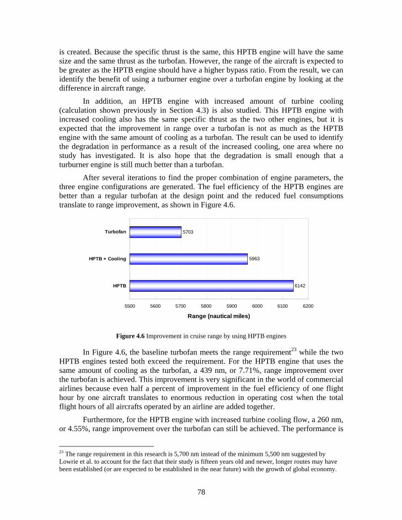
is created. Because the specific thrust is the same, this HPTB engine will have the same size and the same thrust as the turbofan. However, the range of the aircraft is expected to be greater as the HPTB engine should have a higher bypass ratio. From the result, we can identify the benefit of using a turburner engine over a turbofan engine by looking at the difference in aircraft range.

In addition, an HPTB engine with increased amount of turbine cooling (calculation shown previously in Section 4.3) is also studied. This HPTB engine with increased cooling also has the same specific thrust as the two other engines, but it is expected that the improvement in range over a turbofan is not as much as the HPTB engine with the same amount of cooling as a turbofan. The result can be used to identify the degradation in performance as a result of the increased cooling, one area where no study has investigated. It is also hope that the degradation is small enough that a turburner engine is still much better than a turbofan.

After several iterations to find the proper combination of engine parameters, the three engine configurations are generated. The fuel efficiency of the HPTB engines are better than a regular turbofan at the design point and the reduced fuel consumptions translate to range improvement, as shown in Figure 4.6.

6142

5963

5703

5500 5600 5700 5800 5900 6000 6100 6200

HPTB

HPTB + Cooling

Turbofan

Range (nautical miles)

Figure 4.6 Improvement in cruise range by using HPTB engines

In Figure 4.6, the baseline turbofan meets the range requirement23 while the two HPTB engines tested both exceed the requirement. For the HPTB engine that uses the same amount of cooling as the turbofan, a 439 nm, or 7.71%, range improvement over the turbofan is achieved. This improvement is very significant in the world of commercial airlines because even half a percent of improvement in the fuel efficiency of one flight hour by one aircraft translates to enormous reduction in operating cost when the total flight hours of all aircrafts operated by an airline are added together.

Furthermore, for the HPTB engine with increased turbine cooling flow, a 260 nm, or 4.55%, range improvement over the turbofan can still be achieved. The performance is

23 The range requirement in this research is 5,700 nm instead of the minimum 5,500 nm suggested by Lowrie et al. to account for the fact that their study is fifteen years old and newer, longer routes may have been established (or are expected to be established in the near future) with the growth of global economy.

78

indeed inferior to the HPTB engine with less turbine cooling, as expected, but the degradation is not enough to erode the overall superior performance brought by the HPTB. In fact, because the turbine cooling flow in this configuration is 75% more than the HPTB engine with the same cooling flow as the turbofan, the degradation in performance is actually not as large as expected, with only about 40% of the 7.71% improvement over the turbofan being lost because of the additional cooling.

From this result, it would seem that a turburner engine does not lose as much performance as a turbofan engine does when the turbine cooling flow is increased. More calculations are certainly needed to investigate this discovery because one of the major challenges to build a turburner engine is to ensure enough cooling is provided to protect the blade without degrading the performance of the engine too much. This discovery is certainly welcomed as more cooling flow can be supplied while maintaining the performance. These calculations and detailed discussions on how sensitive the performance of a turburner engine is to the amount of cooling flow are presented later in Section 4.6. For the moment, we can only take a note on this discovery then move on to discuss the off-design performance of the three engines investigated.

As mentioned earlier, an engine for supersonic aircraft not only has to have good performance at the supersonic cruise point, it must also provide enough thrust with low fuel consumption rate at other off-design conditions. For this research, there are two transient flight conditions, take-off and transonic acceleration, where the aircraft requires ample thrust. It is also expected that the aircraft will fly subsonically in certain populated areas where noise and shock associated with supersonic flight are unacceptable, so a subsonic cruise condition is specified and the fuel economy at this condition must also be high. Therefore, the off-design performance of the three engines considered are calculated to determine if turburner engine still provide improved performance in these conditions.

During the calculations, it becomes quite clear that all the three engine configurations have no trouble exceeding the thrust requirement in each of the flight conditions. Therefore, all the engines are throttled down until they actually only produce the thrust specified in the requirements. Then, the thrust specific fuel consumption at this thrust level is used for comparison. The comparison of the results is shown in Figure 4.7.

79

1.03

0.82

0.79

0.64

0.99

0.79

0.75

0.61

0.96

0.76

0.71

0.57

0.4 0.5 0.6 0.7 0.8 0.9 1.0 1.1

Supersonic Cruise

TransonicAcceleration

Subsonic Cruise

Take-off

TSFC (lb/hr-lbf)

HPTB

HPTB IC

Turbofan

Figure 4.7 Off-design performance improvement by using HPTB engines

In the figure, one can clearly see that the two HPTB engines considered are more fuel efficient than the turbofan in all four critical flight conditions. This result shows that the range improvement of an aircraft with HPTB engines is going to be even more than the value predicted when only supersonic cruise is considered. An HPTB engine will use less fuel than a turbofan engine almost from the moment the engine starts. Then, the HPTB engine will maintain this edge in fuel economy over the entire flight profile. As a result, the range of the aircraft is being improved over the entire flight profile.

Again, the HPTB engine with increased cooling, represented in the figure as HPTB IC (IC for increased cooling), does not perform as well as the HPTB engine with the same cooling as the turbofan. On the other hand, the improvement is still significant when the cooling is increased. Therefore, we can say that while the increased cooling does degrade the performance of a turburner engine, a turburner engine still performs much better than a turbofan engine in the conditions considered.

As stated earlier, the subsonic cruise condition is critical to realizing a supersonic transport because the aircraft is expected to operate at this condition for a prolonged period of time. The fact that the HPTB engines require less fuel in not only supersonic cruise but also subsonic cruise clearly demonstrate that the an aircraft with HPTB engines can fly much longer range than one with turbofan engines. On the other hand, a corollary of the result is that an HPTB engine can also make engines for subsonic aircraft much more fuel efficient.

The results from preliminary calculations have indicated that a turburner engine has a higher optimum bypass ratio than a regular turbofan. While the calculations are done in a supersonic cruise condition, we argue that it is the fundamental physics – the combustion in an HPTB re-energizing the flow before it enters LPT (low-pressure turbine) – in a turburner that causes this result. Therefore, the result can certainly be applied to subsonic cruise condition. However, application of this discovery to a subsonic

80

aircraft is questionable because the partial throttle performance of a turburner engine has not been established. Since the subsonic aircraft usually cruise at a much lower throttle setting than take-off because the requirement in thrust at the cruise point is not high, it is possible that the benefit brought by turburner is eroded or insignificant in such a condition because there is no demanding requirement in thrust.

From the subsonic cruise performance shown in Figure 4.7, one can clearly see that a turburner engine still maintains its edge in fuel economy over a turbofan when the requirement in thrust is low and low throttle setting is used. Consequently, we can safely say that a turburner engine, especially an HPTB engine where off-design performances have been calculated, is also more fuel efficient than a turbofan if the application is a subsonic aircraft and the engine has a high bypass ratio (even higher than the 5 tested in the preliminary calculations).

From the results discussed above, we can clearly see that an HPTB engine is much more fuel efficient than a turbofan engine for a supersonic aircraft. The reduced fuel consumption rate can either be used to produce a supersonic aircraft that has longer range or used to reduce the operating cost of the supersonic aircraft, leading to an economical supersonic transport for the future. Even if the application is a subsonic aircraft, we expect an HPTB engine to still out-perform a turbofan engine substantially because a turburner engine can be designed with a larger bypass ratio and can maintain the performance edge even in low throttle settings.

More importantly, the results show that the degradation as a result of the increased cooling is not enough to erode the performance improvement brought by using turburners. In fact, the results seem to indicate that increasing cooling does not reduce the performance of a turburner engine as much as that of a turbofan engine. Further calculations on this observation are needed, but the performance improvement of an HPTB engine with increased cooling is still significant to guarantee further research on employing HPTB engines on supersonic aircraft.

4.5 Results for Turburner Engine Optimized for Size

While the results from the previous section are very encouraging, a closer examination of the three engines shows that all three have an engine mass flow rate of about 1,800 lb/s at standard, sea level, static condition. This mass flow rate is roughly the mass flow rate of a 747 engine and the size of the engine is considerable. For a supersonic transport to be realized, not only must the engine produce the required thrust and fuel efficiency, but the airframe must also produce the assumed lift-to-drag ratio at each flight condition. The large size of the three engines considered certainly translates to a larger drag force on the aircraft and the lift-to-drag ratio assumed may become overly optimistic. Consequently, the question may be raised regarding whether it is possible to use four engines of this size to propel a 500,000 lb aircraft.

Indeed, Lowrie et al. [32] only considered engines with mass flow rate up to 1,200 lb/s at standard, sea level, static condition (equivalent to a 757 engine) for the 500,000 lb MTOW (maximum take-off weight) aircraft in their work. However, one must recognize that the requirements set forth in this research are more stringent than those set

81

in their work. As a result, the engine may be somewhat more futuristic than what they had considered. In fact, Lowrie et al. concluded that the configurations they considered, based on then-current technology and then-predicted progress, could not meet the requirements they set. Therefore, it is not surprising that the three engines considered in the previous section are larger than previous study because increasing the bypass ratio is the only way to achieve the desired range requirement.

While there may be hope that some aerodynamic improvement or innovative way to integrate larger engines in a supersonic transport without significant drag penalty can be found, we must consider the situation where the drag of the three engines studied in the previous section prohibits their use on the aircraft considered. In order to reduce the size of the engine, the engine mass flow rate must be reduced while the specific thrust must be increased to compensate for the reduced mass flow. Consequently, the bypass ratio of the engines has to be reduced, leading to a higher TSFC and a shorter aircraft range.

For the baseline turbofan engine, reducing bypass ratio is unpractical as the aircraft range will fall short of the requirement (recalling that the aircraft range only beats the 5,700 nm requirement by 3 nm). For the two HPTB engines, however, their range advantage over the turbofan can certainly be transformed into a size advantage over the turbofan. Therefore, the bypass ratio of both HPTB engines are reduced until the two engines can only produce the required range, 5,700 nm. The engines are then resized to produce the required thrust.

As shown in the preliminary calculations, an HPTB engine has higher specific thrust than a turbofan engine while maintaining almost the same or less TSFC than a turbofan when the bypass ratio is the same. Therefore, it is expected that the two HPTB engines will have very similar bypass ratios to the bypass ratio of the baseline turbofan, but the size of the HPTB engines will be much smaller. As can be seen in Figure 4.8, both HPTB engines indeed behave as expected and are much smaller than the baseline turbofan.

310

349

525

1160

1270

1845

0 200 400 600 800 1000 1200 1400 1600 1800 2000

HPTB

HPTB + Cooling

Turbofan

Mass Flow Rate (lb/s)

Sea Level Static

Supersonic Cruise

Figure 4.8 Reduction in engine size by using HPTB engines

From the figure, it is clear that the turbofan requires significantly more air to provide the needed thrust at the supersonic cruise condition. As a result, the turbofan is much larger and at the sea level it requires more than 1,800 lb/s of mass flow. For both

82

HPTB engines, the required mass flow is much less and at the sea level only around 1,200 lb/s of mass flow is needed. The reduced mass flows translate to 30%~40% reductions in mass flow rate, as shown in Table 4.6. This huge reduction in engine mass flow rate certainly means a much smaller engine can be produced by using turburners.

Table 4.6 Percent reduction in engine mass flow by using HPTB engines

Supersonic Cruise

Sea Level Static

Supersonic Cruise

Sea Level Static

Turbofan 1.0301 5702.8 100.00% 525 1845 0.00% 0.00%HPTB + Cooling 1.0266 5722.3 100.34% 349 1270 -33.52% -31.20%HPTB 1.0153 5786.1 101.46% 310 1160 -40.95% -37.12%

Normalized Range (%)

Engine Configuration

TSFC (lb/lbf-hr) Range (nm)

Mass Flow Reduction (%)Mass Flow Rate (lb/s)

In the table, one can clearly see that the HPTB engine without additional cooling provides the most reduction in engine mass flow, with nearly 41% at supersonic cruise. For the HPTB engine with increased cooling, a 33.5% reduction in engine mass flow can still be achieved. Again, the difference in performance between the two HPTB engines is not as pronounced as expected, considering that one configuration has a 75% increase in cooling flow over the other one that has the same amount of cooling as the turbofan case. Certainly, the effect of cooling flow on the performance of a turburner engine should be investigated further because the results from this section and the previous section all show that the degradation in performance is not as much as expected. Again, this discussion will be provided in the next section.

One will notice from Figure 4.8 and Table 4.6 that the reduced mass flows in the HPTB engines match the mass flow rates of the engines considered by Lowrie et al. very well (all in the range of 1,200 lb/s), so the drag associated with the two HPTB engines is certainly within acceptable range and will not invalidate the assumptions on the lift-to-drag ratio of the aircraft. Furthermore, one should recall that the engines considered by Lowrie et al. did not produce low enough TSFC to meet the requirement (a 5,500 nm range) in their work, but the two HPTB engines actually meet the more stringent requirement of a 5,700 nm range in this research. As a result, it is evident that an HPTB engine is vastly superior to a turbofan engine for a supersonic aircraft.

From the above results, one can safely say that an HPTB engine is a much better propulsion choice than a turbofan for a supersonic transport because of the reduced drag of a smaller engine. If the baseline turbofan is too large to satisfy the assumption regarding lift-to-drag ratio of the aircraft, the HPTB engines certainly can be made smaller to ensure the validity of the assumption while meeting all the requirements. On the other hand, it would be interesting to see how the off-design performance of the HPTB engines varies because of two reasons.

One of the two reasons is that the engine mass flow rate is much lower in the two HPTB engines, so the engines are more sensitive to any change in specific thrust caused by the change in flight conditions. For some off-design conditions that require high thrust, it is possible that higher throttle settings may be needed. As a result, the TSFC may be higher.

83

The other reason is that the bypass ratios of the two HPTB engines are much smaller than the cases considered in the previous section. In the discussions on the results from the preliminary calculations, we have shown that an HPTB engine will provide significant increase in specific thrust over a turbofan regardless of the bypass ratio. However, the TSFC of an HPTB engine in lower bypass ratio may be slightly higher than a turbofan, but the TSFC of an HPTB engine will decrease more rapidly than a turbofan as the bypass ratio is increased. We conclude that an HPTB engine is the best choice for further considerations, but it will provide more improvement with larger bypass ratios. Therefore, the off-design performance of the HPTB engines considered in this section may not behave the same as the HPTB engines considered in the previous section because the differences in their bypass ratios.

The off-design calculations are carried out in the same manner as the off-design calculations presented in the previous section. For each of the critical flight conditions, each engine is throttled down until only enough thrust is generated. The resulting TSFC from each configuration is compared, as shown in Figure 4.9, to see which engine provides the lowest TSFC in each flight condition. The results are quite interesting, but not completed unexpected.

1.03

0.82

0.79

0.64

1.03

0.85

0.79

0.69

1.02

0.85

0.77

0.69

0.4 0.5 0.6 0.7 0.8 0.9 1.0 1.1

Supersonic Cruise

TransonicAcceleration

Subsonic Cruise

Take-off

TSFC (lb/hr-lbf)

HPTB

HPTB IC

Turbofan

Figure 4.9 Off-design performance of HPTB engines with reduced mass flow

In the figure, one can see that the two HPTB engines have almost the same TSFC as the baseline turbofan at the supersonic cruise condition because we force the engines to produce the same range as the turbofan. The same can also be said about the subsonic cruise condition because the TSFC of all three engines are almost the same, although the HPTB engine with increased cooling actually has a slightly higher TSFC than the turbofan. From the two cruise conditions, one would expect the two HPTB engines with reduced mass flow will still produce roughly the same cruise range as the baseline turbofan.

84

However, both HPTB engines have higher TSFC than the turbofan in the two transient flight conditions, unlike what has been observed from the results shown in the previous section. The increase of TSFC in the transient conditions is certainly undesirable as the range of the aircraft will decrease. Fortunately, the decrease in range should be small as the higher TSFC occurs at transient flight conditions. Furthermore, one must keep in mind that the reason to produce the two HPTB engines with lower bypass ratio is that the mass flow rate of the baseline turbofan may be too large and produce too much drag. If the turbofan is indeed deemed too large in a more thorough analysis on the integration of propulsion and airframe, the lower TSFC of the turbofan is meaningless because the baseline turbofan simply cannot be put into the supersonic transport designed.

Nonetheless, the higher TSFC of HPTB engines at transient conditions should be investigated further to determine what factors have contributed to the increase. Because we have suspected that the two HPTB engines are more sensitive to the change in specific thrust and higher throttle setting may be needed, the throttle settings are first examined, as shown in Table 4.7.

Table 4.7 Variation of throttle setting in the critical flight conditions

Turbofan HPTB HPTB + Cooling

2.00 60000 12500 3078 3078 30781.20 40000 25000 2867 2981 29890.95 36000 8500 2025 2171 21870.30 0 50000 2649 2835 2835

Mach Number

Altitude (ft)

Thrust (lbf)

Throttle Setting, Tt4 (R)

One can immediately recognize from the data in the table that the two HPTB engines indeed have higher throttle settings than the turbofan in the three critical off-design conditions. Again, this discovery is not unexpected because the HPTB engines are using much less air than the turbofan and therefore cannot accept the large variation in specific thrust associated with larger throttle changes. However, the higher throttle settings cannot explain why the HPTB engines only have higher TSFC than the turbofan in the two transient conditions as both HPTB engines operate with higher throttle settings in all three off-design conditions considered. Consequently, we must examine the change in bypass ratio of the HPTB engines in off-design conditions – the other factor that we believe could cause a very different behavior in off-design for the two engines. These values of bypass ratio in different flight conditions can be found in Table 4.8.

Table 4.8 Variation of bypass ratio in the critical flight conditions

Mach Number Altitude (ft) Thrust (lbf) Turbofan HPTB Range + CoolinHPTB Range

g HPTB Size CoolinHPTB Size +

g2.00 60000 12500 1.70 4.00 3.40 1.70 1.701.20 40000 25000 1.27 3.29 2.74 1.40 1.380.95 36000 8500 1.79 4.75 3.99 2.02 2.000.30 0 50000 1.49 3.87 3.23 1.59 1.58

In the table, the two HPTB engines optimized for longer range, discussed in previous section, are labeled as “HPTB Range” while the two HPTB engines with less

85

mass flow rate are labeled as “HPTB Size”. One can clearly see that, in general, the bypass ratios in the two transient flight conditions are lower than those at the design point (supersonic cruise), while the bypass ratios in the subsonic cruise condition are higher than those at the design point. Among all the HPTB configurations and flight conditions considered, the two HPTB engines with reduced size have the smallest bypass ratio in the transient conditions. At the same time, only these two engines in the transient conditions produce a higher TSFC than the baseline turbofan. Therefore, it would appear that the higher TSFC of the two HPTB engines with reduced mass flow in the transient conditions are caused by the smaller bypass ratios experienced by the engines.

Recalling that we have shown that an HPTB engine has a higher optimum bypass ratio than a turbofan and that the improvement of an HPTB engine over a turbofan will increase with the increasing bypass ratio, the results are certainly not unexpected. For the two transient conditions considered, the bypass ratio of both HPTB engines with reduced mass flow is too small and too far away from the optimum bypass ratio (which should be a larger value) of an HPTB engine. At the same time, the turbofan, which has a smaller optimum bypass ratio in general, does not suffer as much penalty when the bypass ratio is reduced in the two conditions. Consequently, while the two HPTB engines still produce much higher specific thrust than the turbofan in these conditions, the TSFC of the two engines are higher than that in the turbofan – very similar to what have been observed in the case with bypass ratio of one in the preliminary calculations, where turburner engines produce much better specific thrust at the cost of slightly increased TSFC over a turbofan.

From these results and discussions, we believe that the higher TSFC of the two reduced-sized, HPTB engines in the transient conditions is indeed caused by their smaller bypass ratios. Again, if the baseline turbofan engine is too large for the aircraft considered, the higher TSFC of the HPTB engines in transient conditions is not a liability anyway. However, this discovery certainly matches well with our observations and arguments made earlier regarding the turburner engines in general – a turburner engine has higher optimum bypass ratio than a turbofan and the difference in performance is between the two is larger at higher bypass ratios.

On the other hand, this investigation into the cause of higher TSFC of HPTB engines in certain off-design conditions also shows another interesting, and very useful, behavior of a HPTB engine in off-design conditions. A closer examination of Table 4.8 reveals that the two reduced-sized, HPTB engines actually have less reduction in bypass ratio than the turbofan between the design point and the take-off condition. The variation in bypass ratio for the two HPTB engines (in the right most columns) between the two conditions is about 0.11, while the variation for the turbofan is twice as much as those in the HPTB engines, at 0.21. This smaller variation in bypass ratio of the HPTB engines can also helps HPTB engines to become a much better engine for supersonic aircraft than turbofans.

One of the challenges in producing an engine for supersonic aircraft lies in the variation of bypass ratio in different flight conditions. The engine is desired to have large bypass ratio at take-off and low speed to take advantage of the fuel economy brought by the larger bypass ratios. As the aircraft accelerates and eventually reaches the supersonic cruise condition, the bypass ratio of the engine is desired to be small to produce sufficient

86

thrust. Unfortunately, the natural off-design variation of bypass ratios with respect to the change of flight conditions is actually the other way around – the bypass ratio is smaller at take-off and increases to a larger value at supersonic cruise, as evidenced in the data shown in Table 4.8. Because of this variation in bypass ratio, designers face immense challenges to find an optimum engine design for a supersonic aircraft – picking a small bypass ratio at supersonic cruise sacrifices low-speed economy and choosing a large bypass ratio at low-speed means not enough thrust at supersonic cruise.

To overcome this challenge, scientists and engineers have embraced the idea of “variable cycle engines”, where the bypass ratio of the engine is artificially changed (through complicated internal ducting and valve system to block or bleed off the bypass stream) in different flight conditions. While the concept has been proven practical and actual engines have been used to propel prototype aircraft (in the form of YF-22A and YF-23A fighters), the mechanical complexity of the system and the associated cost prevent the wide spread use of such engines. As far as supersonic transport is concerned, several studies have proposed to use such engines to propel next generation supersonic transports, including the work by Lowrie et al., to overcome the natural, but adverse, variation of bypass ratio.

In addition to the complexity of the system, variable cycle engines face another problem. As mentioned earlier, the variable cycle engines considered by Lowrie et al. still did not meet the requirements set in their work. They concluded that the deficiency of their engines lies in the fuel economy of both supersonic and subsonic cruise. The reason is quite simple. While the turbojet mode of their engines did provide enough thrust in supersonic cruise, this mode simply could not produce the desired fuel economy and the aircraft had to rely on subsonic cruise to achieve the overall range desired. However, because the subsonic cruise speed is less than half of the supersonic speed, the fuel consumption rate must be lowered to less than half of that at the supersonic cruise to reach the same range. Unfortunately, the change in bypass ratio in the variable cycle engines was still not large enough to produce the required reduction in TSFC.

Clearly, to actually employ variable-cycle engines in a supersonic transport, even more complicated systems that allow the engines to still operate as low bypass turbofan are needed. On the other hand, we have demonstrated that the HPTB engines can produce the same thrust as turbofans while lowering the fuel consumption rate. Such capability in itself makes HPTB engines highly suitable for supersonic aircraft. The fact that HPTB engines experience only half of the variation in bypass ratios in turbofans only adds to the superiority of HPTB engines. Because using HPTB engines significantly alleviates the problem associated with the varying bypass ratios, variable cycle systems can be completely dispense with while still maintaining desired performance over the entire flight profile.

In order to demonstrate this discovery further, a summary of the variations in bypass ratio with respect to the change in flight conditions is created and shown in Table 4.9. Notice that all the data are generated with maximum throttle setting, turbine inlet temperature equals 3,240 R, to ensure only the variation caused by change in flight condition is included. Consequently, some values are slightly different from the values shown in Table 4.8. Also, the two HPTB engines optimized for longer range, discussed in

87

previous section, are labeled as “HPTB Range” while the two HPTB engines with less mass flow rate are labeled as “HPTB Size”.

Table 4.9 Bypass ratio variations in different flight conditions (Tt4 = 3,240 R)

Mach Number Altitude (ft) Turbofan Variation (%) HPTB Size Variation (%) CoolinHPTB Size +

g Variation (%)

2.00 60000 1.59 40.00% 1.56 21.14% 1.55 22.50%1.60 50000 1.30 14.85% 1.37 6.66% 1.36 7.23%0.00 0 1.13 0.00% 1.28 0.00% 1.27 0.00%

Mach Number Altitude (ft) Turbofan Variation (%) HPTB Range Variation (%) HPTB Range + Cooling Variation (%)

2.00 60000 1.59 40.00% 3.66 22.54% 3.10 24.25%1.60 50000 1.30 14.85% 3.21 7.25% 2.69 7.87%0.00 0 1.13 0.00% 2.99 0.00% 2.50 0.00%

One can clearly see from the table that all HPTB configurations have an increase in bypass ratio in the range of 20~25% over the bypass ratio at sea level static condition when the engines are flying at supersonic cruise condition. This increase, however, becomes 40% in the case of turbofan. The difference between the turbofan and the HPTB engines is very similar to what has been shown earlier with the data in Table 4.8. Again, this reduced increase in bypass ratio for the HPTB engines means that an HPTB engine can maintain high thrust at high cruise speed while ensuring fuel efficiency in different flight conditions, offering a much better propulsion source for the supersonic aircraft.

Similar comparison can be found in the flight condition of Mach 1.6 at 50,000 ft. The increase in bypass ratio from sea level static condition is about 15% now for the turbofan, much less than the 40% increase observed in the supersonic cruise condition. On the other hand, the HPTB engines still only have roughly half as much increase as the turbofan, with only 6.7~7.9% increase from the sea level static condition.

From the data of the two supersonic flight conditions, one would expect that the degradation in thrust caused by increased bypass ratio for a turbofan is going to be even more severe as the aircraft flies to a higher Mach number and altitude. At the same time, an HPTB engine will still has roughly half as much increase in bypass ratio as a turbofan in these flight conditions. As a result, an HPTB engine is an even better choice than a turbofan for a supersonic aircraft designed to fly at higher Mach number and altitude because the aircraft has a more demanding thrust requirement at higher flight Mach numbers and a smaller bypass ratio at the cruise point is needed.

In a summary to this section, we have demonstrated that an HPTB engine can be made much smaller than a turbofan while delivering the same fuel efficiency. The reduction in size should address the doubt that the baseline turbofan engine may have more drag than assumed. The results from the off-design performance also reinforce our earlier conclusion that an HPTB engine has a higher optimum bypass ratio than a turbofan and its performance improvement over a turbofan increases as the bypass ratio is increased.

A closer examination on the variation of the bypass ratio with respect to change in flight condition shows that an HPTB engine has much smaller increase in bypass ratio than a turbofan as the aircraft moves to higher flight speed and altitude. Consequently, an HPTB engine presents a much better choice than a traditional turbofan as well as a

88

variable cycle turbofan because it can maintain high thrust and good fuel efficiency at high speed. It is also expected that this advantage will become more prominent when the design cruise speed and altitude are higher than the Mach 2, 60,000 ft considered in this research.

4.6 Sensitivity of Engine Performance to Turburner Cooling

In the previous two sections, the advantages of employing turburner engines in a supersonic transport are examined. The results clearly show the superiority of the HPTB engines over the baseline turbofan, even if the amount of turbine cooling is increased. While the fact that an HPTB engine with increased cooling can still perform better than a turbofan is good enough for our purpose, we have observed that the performance of HPTB engines does not seem to be as sensitive to the amount of turbine cooling as expected. In this section, this sensitivity is examined and the results will demonstrate another important characteristic and advantage of turburner engines previously undiscovered.

For a turbofan engine to achieve high performance, turbine cooling is a must because it is the only way to allow higher combustion exit temperature, which determines the thermal efficiency of the cycle. On the other hand, the amount of turbine cooling has to be minimized because the cooling air does not go through the combustion process and therefore does not produce Brayton cycle work. While the amount of cooling flow can affect performance through other realistic effects, such as larger mixing losses associated with more cooling flow, the amount of cooling flow affect the engine performance mostly through varying the thermodynamic cycle fundamentally – diverting a smaller amount of flow before the combustor (and does no Brayton cycle work) to allow the rest of the flow to produce more Brayton cycle work by reaching a higher combustor exit temperature. As a result, higher cycle performance can be achieved if less cooling flow is needed for a given combustor exit temperature and numerous work have been done to investigate and improve turbine cooling techniques.

When the turburner concept, which introduces combustion within turbine, is proposed, it is expected that the amount of cooling will be increased because of the higher temperature associated with combustion. Naturally, it is also expected that the performance will degrade as the amount of cooling is increased because it is what has been experienced in a gas turbine engine. However, this expectation is not entirely founded, as the results in the previous two sections have shown.

The reason for these somewhat unexpected results is actually deceptively simple, but counter-intuitive. For an engine with turburners in place of turbines, the cooling flow diverted before the entrance to the main combustor still can not produce Brayton cycle work, the same as the cooling flow in a regular turbofan engine. However, after the cooling flow enters the turburner, the flow has another chance to receive heat from the combustion in the turburner and then use the energy received to drive the turbine. As a result, the cooling flow supplied to a turburner actually generates cycle work, the same as the main hot stream from the main combustor. The work generated by “burning” the cooling flow is certainly less than the work generated by the hot stream because the heat

89

addition takes place in a lower temperature. However, the fact that the cooling flow is producing cycle work in a turburner – when the cooling flow into a regular turbine does no cycle work – simply means that the performance of a turburner engine is more resistant to the degradation caused by increased cooling flow than a turbofan. In other words, the performance of a turburner engine is less sensitive to the change in the amount of cooling than a turbofan.

In a sense, the cooling flow in a turburner acts like a combination of the dilution flow in the main combustor and the cooling flow in a regular turbine. In order to ensure the acceptable ignition and flammability characteristics, only a small potion of the flow entering the main combustor goes directly into the primary zone where the flame is ignited and held. The rest of the flow enters the main combustor through the dilution holes later on to complete the combustion and provide cooling of the casing.

The amount of the dilution flow certainly does not affect the cycle performance, with the exception of mixing losses, because the dilution flow is being heated by combustion as well, albeit somewhat indirectly. Ideally, the flow at the exit of combustor has completed all the combustion and mixing so the flow can be represented as a uniform flow with a uniform temperature distribution. Therefore, from the cycle analysis point of view, the dilution flow produces cycle work in the same way as the small portion of the flow that actually goes through the primary combustion zone because of the averaged, uniform flow condition at the exit.

From this observation on the dilution flow in the main combustor, one can certainly say the same about the cooling flow in a turburner. Because there is combustion in a turburner, the cooling flow can react and mix with the fuel and the hot stream. If the exit condition can be made such that the average exit temperature is the same, then, ideally, how much flow enters the turburner through the main flow pass and how much flow enters the turburner through cooling holes do not affect the cycle performance. Granted, there are realistic effects that would still penalize a larger cooling flow, but the analogy to dilution flow certainly reinforces the argument that a turburner engine is more resistant to the degradation of performance caused by the increased cooling flow than a turbofan.

Another example can also demonstrate the fact that a turburner engine does not suffer as heavy penalty as a turbofan when the amount of cooling is increased. Let us consider the extreme case where all the compressor flow is diverted before entering the main combustor and used as cooling flow. Obviously, a turbofan engine cannot run in this situation because there is no air going through the combustor and no combustion, a necessary step to complete the Brayton cycle, is present in the engine. Therefore, no work is generated in this extreme case because no air is going through the Brayton cycle to produce work.

For a turburner engine, this case simply reduces the engine to a Ramohalli cycle [4], where the turburner replaces both the main combustor and the traditional turbine. As mentioned earlier, the cycle considered in Ramohalli’s work is unpractical because he assumed the compressor exit temperature to be the much higher turbine inlet temperature. In this case where all compressor exit flow is used for cooling, the turbine inlet temperature is assumed to be the much lower compressor exit temperature so there is no

90

technical difficulty associated with the assumption of temperatures24 . As a result, a turburner engine will still work in this extreme case and produce cycle work.

Considering the enormous difference between a turburner engine and a turbofan with the same amount of cooling in this extreme case (the percent difference is actually infinity because a turbofan produces zero work), it is certainly expected that the performance of a turburner engine will degrade much slower than a turbofan with the increase of cooling flow, eventually reaching the theoretical maximum difference.

With the results from the previous two sections and the observations made in the above paragraphs, the evidence to support the argument that a turburner engine is more resistant than a turbofan to the degradation in performance brought by increased cooling is certainly strong. However, some more calculations are carried out to complete the investigation and provide a quantitative expression of the argument.

To show that the cooling flow supplied into a turburner indeed degrades the engine performance less than when the same amount of cooling flow is supplied to a turbine, the amount of cooling supplied to an HPTB engines and a turbofan is varied to see the change in engine performance. Specifically, the case with a bypass ratio of one in the preliminary calculations is used. The engines considered in that case have 17.5% of the compressor exit flow supplied to the high-pressure turbine (HPT) or the high-pressure turburner (HPTB) and 2.5% of the compressor exit flow is used to cool the low-pressure turbine (LPT)25. The amount of cooling flow supplied to the high-pressure section is varied with a 5% interval initially and a 10% interval in after more than 40% of compressor air is used for cooling, beyond the maximum amount for turbine cooling practiced currently. For all the data points, the bypass ratio is forced to remain unity in order to avoid the variation in performance brought by the bypass ratio. The calculated data of each engine are then normalized by the maximum performance achieved by each engine (when the amount of cooling is minimal), respectively, to show the percent degradation in performance plotted in Figure 4.10.

24 Granted, there is no need to cool the turbine in this case anyway. 25 There is also 1% of the compressor air used as bleed air to drive other component in the aircraft. Coupled with the fact that the components also have realistic efficiencies, the maximum amount of cooling that can be supplied to turbine is limited and the extreme case with 100% compressor air used for cooling can not be included. In fact, the calculations have to be stopped when the fan pressure ratio reaches one, which means the LPT does not exit, contradicting the assumption that cooling is supplied to LPT.

91

-100%

-90%

-80%

-70%

-60%

-50%

-40%

-30%

-20%

-10%

0%

0 10 20 30 40 50 60 70 80 90 10

HPT Cooling Flow (Percent of HPC Exit Flow)

Spec

ific

Thru

st D

egra

datio

n

0

Turbofan

HPTB

Figure 4.10 Degradation in performance as a function of HPT cooling

It is immediately apparent from the figure that the degradation of specific thrust with respect to the increasing cooling in an HPTB engine is indeed much less than that in a turbofan. From the data points where 22.5% and 37.5% of compressor air are used to cool the high-pressure section, one can see that the performance degradation in an HPTB engine is half as much as that in a turbofan. The halved degradation when the same amount of cooling is supplied also means that close to twice the amount of cooling can be supplied into an HPTB for the same amount of performance degradation as in a turbofan. This corollary can be seen by finding the intercepts of the two curves with the horizontal gridlines of constant performance degradation. An example is that, at the 10% degradation gridline, 20% of compressor air is supplied to the HPTB in the turburner engine, but only 12% of compressor air is supplied to the HPT in a turbofan.

The results shown in the figure provides a clear support to our argument that the cooling flow supplied into a turburner still does a cycle work and the performance of a turburner engine is less susceptible to the adverse effect caused by increased cooling. In itself, this discovery allows the designers to use more cooling flow to protect turbine blades against the newly introduced combustion without fearing the performance penalty, a major concern for the scientists and engineers that work on turbine cooling.

One must also keep in mind that the data are normalized by the maximum specific thrust achieved by each engine respectively. As a result, the actual percent difference in performance between the HPTB engine and the turbofan can not be directly observed from the figure. As shown in the preliminary calculations, the HPTB engine has a 59% performance improvement over the turbofan when the same 20% of compressor air is used for cooling. We have also predicted that in the extreme case where all compressor air is used for cooling, the performance improvement brought by using HPTB over regular HPT is infinite. Therefore, it is interesting to see if the values calculated can validate this postulation and show that the performance advantage from using HPTB actually increases with increasing amount of cooling. Indeed, the data shows the prediction to be true, as shown in Table 4.10.

92

Table 4.10 Performance advantage of HPTB engines over turbofans

HPT Cooling (%)

LPT Cooling (%) Specific Thrust

Turbofan

(lbf-s/lbm)

HPTB Specific Thrust (lbf-s/lbm) Performance

De

Turbofan

gradation (%)

HPTB Performance

Degradation (%)

Performance Advantage of HPTB Engine

2.5 2.5 37.3174 54.5115 0.00% 0.00% 46.08%7.5 2.5 35.3877 53.0426 -5.17% -2.69% 49.89%

12.5 2.5 33.4185 51.5092 -10.45% -5.51% 54.13%17.5 2.5 31.3980 49.9935 -15.86% -8.29% 59.23%22.5 2.5 29.3239 48.4497 -21.42% -11.12% 65.22%27.5 2.5 27.1924 46.8519 -27.13% -14.05% 72.30%32.5 2.5 25.0084 45.2310 -32.98% -17.02% 80.86%37.5 2.5 22.7502 43.5954 -39.04% -20.03% 91.63%47.5 2.5 17.9890 40.1986 -51.79% -26.26% 123.46%57.5 2.5 12.8214 36.6522 -65.64% -32.76% 185.87%67.5 2.5 7.0125 32.7713 -81.21% -39.88% 367.33%

From the table, it is quite evident that both the HPTB engine and the turbofan suffer from the performance penalty of turbine cooling, but the HPTB engine is able to maintain higher performance as the cooling is increased. In fact, looking at the right most column, the performance advantage of the HPTB engine starts to increase rapidly and non-linearly at higher cooling flow. Although the code forbids further increase in cooling flow because of the reasons explained earlier, one can certainly see that the trend should lead to an eventual infinity of performance advantage when all compressor air is used for cooling. As a result, the performance advantage of an HPTB engine over a turbofan actually increases with increasing cooling flow, if the same amount of cooling is assumed for both engines.

In fact, by looking at the actual specific thrust produced by the turbofan with minimal cooling (2.5% for HPT and 2.5% for LPT), one realize that an HPTB engine would only produce such low performance when close to 57.5 of compressor air is supplied to cool the HPTB. The increase in the amount of cooling supplied to the high-pressure section is actually 23-fold until the performance of an HPTB engine is brought down to the same performance as a turbofan. This discovery certainly shows that the increased cooling in a turburner is almost a non-issue as far as performance is concerned.

From the above results, we can conclude that a turburner engine will still out-perform a turbofan engine even if the cooling flow supplied to the turburner is doubled or tripled. This conclusion is based on the fact that a turburner engine not only performs much better than a turbofan when no cooling is considered, but also suffers less amount of penalty in performance when the cooling to the turburner is increased. Consequently, scientists and engineers can use more cooling flow than previously thought possible, based on the experiences with turbofan, in a turburner engine while still producing a much better performing engine than a turbofan.

On the other hand, looking back at the results shown in the previous two sections, the HPTB engine with increased cooling still suffers noticeable, but less than expected, performance penalty. The results certainly seem to contradict what we have concluded here about the amount of cooling supplied to the turburner has very little effect on performance. A closer examination of the HPTB engine considered previously show that most of the increase in cooling flow is supplied to the LPT to counter the significantly hotter stream leaving the HPTB. Although we believe the amount of cooling supplied to a

93

turburner does not affect the performance much because there is still combustion within the turburner, the regular LPT (no combustion) in the HPTB engine considered in the previous two sections certainly does not benefit from this conclusion. As a result, the amount of cooling flow supplied to the LPT in the HPTB engine, which is significantly larger than that in a turbofan, still degrade the engine performance in a fashion similar to that in a turbofan.

To understand how sensitive the engine performance is to the distribution of cooling flow to the different sections of the turbine, the amount of cooling supplied to the case discussed in Section 4.4, where turburners are used to produce engine with longer range, is varied. In this case, bypass ratio and fan pressure ratio are varied after the amount of cooling has been changed to produce the maximum possible range in the new configuration.

This approach is a departure from the case shown earlier where the effect of bypass ratio is purposefully eliminated. Unlike the previous case, where the purpose is to discover the performance variation caused by the fundamental difference between a turburner and a turbine, we are interested to know here how the amount of cooling in each component affects the engine design and performance. Because changing the distribution inevitably results to a change in the optimum combination of bypass ratio and fan pressure ratio, the bypass ratio and fan pressure ratio must be varied as well to reflect the fact that an optimum design can only be reached when all factors are considered.

Similar to the case discussed earlier in this section, cooling flow is increased in a 5% interval to different turbine sections of the HPTB engine and the turbofan. The total amount of compressor air used for turbine cooling is limited to between 20% and 35%, the two values of cooling flow considered in Section 4.4. The results from the calculations are shown in Table 4.11.

Table 4.11 Performance variation when cooling increased in different components

HPT Cooling (%)

LPT Cooling (%)

Turbofan TSFC (lb/lbf-hr)

HPTB TSFC (lb/lbf-hr)

Turbofan TSFC Increase (%)

HPTB TSFC Increase (%) of HPTB Engine

TSFC Reduction

(%)17.5 2.5 1.0301 0.9564 0.00% 0.00% 7.15%22.5 2.5 1.0409 0.9601 1.05% 0.39% 7.76%27.5 2.5 1.0541 0.9644 2.33% 0.84% 8.51%32.5 2.5 1.0700 0.9693 3.87% 1.34% 9.42%

HPT Cooling (%)

LPT Cooling (%)

Turbofan TSFC (lb/lbf-hr)

HPTB TSFC (lb/lbf-hr)

Turbofan TSFC Increase (%)

HPTB TSFC Increase (%)

TSFC Reduction of HPTB Engine

(%)17.5 2.5 1.0301 0.9564 0.00% 0.00% 7.15%17.5 7.5 1.0619 0.9645 3.08% 0.85% 9.17%17.5 12.5 1.1041 0.9747 7.19% 1.91% 11.73%17.5 17.5 1.1707 0.9873 13.65% 3.23% 15.67%19.0 16.0 0.9852 3.01%

From the table, the conclusion of increased cooling into a turburner reduces the performance less than that into a turbine, from the case discussed earlier, can still be seen. Looking at the upper half of the table where increased cooling is only supplied to the HPT or HPTB, one can see that the difference in the performance degradation between the turbofan and the HPTB engine is actually larger than what have been observed earlier. The degradation in the turbofan is at least 2.5 times of that in the HPTB engine in all cases, compared to the almost twice ratio between the two engines observed earlier.

94

This more pronounced difference is certainly because the fact that now the bypass ratio and fan pressure ratio are varied to produce an optimum design after the amount of cooling has been changed.

For the lower half of the table where all the increased cooling enters the LPT, the degradation of performance is much larger than when the increased cooling enters the HPT or HPTB. The reason of this further degradation is because the fact that the main stream entering the LPT is not as hot as that entering the HPT. The low energy state of the main stream is undesirable in itself because more pressure reduction (or a higher pressure ratio when inlet pressure is divided by exit pressure) is needed to supply the work to drive the fan. When increased amount of cooling is added, the energy state of the main stream is further reduced and more pressure reduction is needed. Consequently, increasing cooling in LPT degrades the performance much more than increasing cooling in HPT.

While this discovery is undesirable for the HPTB engine considered, a closer examination of the data shows that the HPTB engine only receives a third of the performance penalty the turbofan receives when the LPT cooling flow is increased. In fact, the performance penalty when LPT cooling flow in the HPTB engine increases is very similar (slight less actually) to the penalty when HPT cooling flow in the turbofan increases. Considering the reasoning in the previous paragraph, this discovery is not entirely surprising. Because combustion is present in the HPTB engine and maintains the flow at a high temperature at the exit of HPTB (ideally the same as the temperature at the inlet), the LPT in an HPTB engine actually receives a hot stream that is very similar to that received by the HPT in a turbofan. This hot stream requires additional cooling for the LPT, but at the same time the effect of cooling on the engine performance is much more similar than adding cooling to the HPT than to the LPT in the turbofan.

Looking at the last row of Table 4.11 where the data from the increased cooling flow case considered in Section 4.4 is provided as a reference, we can see that most of the degradation in performance observed from the results of that case is the result of the significantly increased cooling flow to the LPT. The cooling flow in the HPTB actually does not increase much and its effect on the performance is almost negligible. Additional cooling can certainly be introduced into HPTB without noticeable performance penalty if the temperature non-uniformity in the HPTB requires more cooling flow to protect the blades.

From the above results, the main factor behind the performance degradation in the HPTB engines with increased cooling considered in the previous two sections has been identified. The significantly increased cooling in the LPT is the key reason behind the performance degradation. The increased cooling in the HPTB is small and its effect is even smaller. Coupled with the other results presented in this section, it would appear that using both HPTB and LPTB in an engine can almost eliminate the concern on degraded performance because of increased turbine cooling. In fact, it is possible that the turbine inlet temperature currently thought achievable can be increased further because more cooling is available, leading to an even more powerful engine.

Unfortunately, this discovery can not be applied directly to this research because the HPTB engine still offers better fuel economy at lower bypass ratios. However, one

95

must realize that the reason to keep the bypass ratio low is to maintain enough thrust while keeping the engine small to meet the assumed lift-to-drag ratio of the overall aircraft. It is possible that an engine with both an HPTB and LPTB can simply reduce the engine size so much that the assumptions made about the lift-to-drag ratio are too pessimistic and less thrust is actually required. Therefore, future research should certainly incorporate this program into a larger multi-disciplinary design optimization where the lift-to-drag ratio of the aircraft can be evaluated at the same time when engine configuration is varied in order to investigate this possibility. After such optimization is carried out, it may show that the configuration where both HPTB and LPTB are used is the best choice because the configuration provides good performance and is almost unsusceptible to the performance degradation caused by increased cooling.

From the discussions in this section, the sensitivity of engine performance to the amount of turbine cooling flow has been established. If the cooling flow is supplied to a turburner instead of a regular turbine, cycle work can still be produced by the cooling flow and the performance degradation is much smaller than (or less than half of that) when the cooling is supplied to a turbine. Considering with that a turburner engine produces much better performance than a turbofan when no cooling is considered, an astronomical, if not unrealistic, amount of increased cooling must be supplied to the turburners in a turburner engine to completely negate the performance improvement introduced by using turburners. Consequently, scientists and engineers working on turbine cooling should have ample amount of cooling flow to tackle the higher flow temperature expected in a turburner.

On the other hand, the HPTB engines considered for a supersonic aircraft in this research is not immune to the performance degradation because most of the increased cooling is supplied to the LPT. However, the HPTB engines will not face any more difficulty in terms of achieving desired performance than current turbofans because the flow entering their LPT is actually much more similar to the flow entering the HPT of turbofans. As a result, the performance degradation will still be manageable and will not erode completely the overall performance improvement of employing turburners.

4.7 Summary

With the discussions on the relationships between engine performance and amount of cooling completed, all the calculated results and planned discussions have been presented. Because much has been covered in this chapter, a summary of findings is presented here.

For a turburner engine, we have found out several trends regarding its performance variation with respect to several engine parameters.

1. A turburner cycle is a more efficient cycle and produces more power than a turbofan cycle. The superiority of a turburner cycle can be used to produce a more powerful and fuel efficient engine.

2. The performance advantage of a turburner engine over a turbofan increases with the increase in bypass ratio. The reason behind this trend is the fact that the flow

96

driving the low-pressure turbine has much more energy in a turburner engine than a turbofan, allowing more efficient use of energy to drive the fan.

3. A turburner engine has a higher optimum bypass ratio than a turbofan, a corollary of previous finding.

4. A turburner engine has the potential to be used in an ultra-efficient subsonic aircraft, in addition to the supersonic aircraft considered. This observation is based on the fact that a turburner engine has a higher optimum bypass ratio than a turbofan and a turburner engine provides more performance improvement over a turbofan as the bypass ratio increases.

5. The amount of cooling flow for a turburner has a much less (at least halved) effect than that for a turbine on engine performance degradation. The reason for this phenomenon is believed to be the fact that the cooling flow entering a turburner can still do cycle work, unlike the cooling flow entering a turbine. As a result, a turburner can use roughly twice the amount of cooling of a turbine before suffering the same engine performance penalty.

6. Because a turburner engine has higher performance when no cooling is considered and suffers smaller penalty when the cooling flow is increased when compared to a turbofan, the performance advantage of a turburner engine over a turbofan is almost impossible to be completely eroded by increased cooling.

7. In off-design performance, the increase in bypass ratio from take-off to supersonic cruise for a turburner engine is only half of that in a turbofan. As a result, a turburner engine can maintain high thrust at high speed while maintaining high fuel efficiency at low speed. This trend alleviates, and potentially eliminates, the need to employ a variable cycle engine, which faces high fuel consumption problem in turbojet mode and is a mechanically complicated system, for supersonic aircraft.

In addition to these generic trends of a turburner engine, several findings on using a turburner engine in the application of most interest, a supersonic transport, have also been concluded.

1. For the supersonic transport considered, the best engine configuration is an HPTB engine, where only a high-pressure turburner is used to drive the high-pressure compressor. This choice is based on the fact that an HPTB engine offers the best improvement over a turbofan in lower bypass ratios, which are expected in order to reduce the size of the engine and therefore the drag of the engine.

2. The results show that significant reduction in engine size and significant increase in aircraft range can be achieved by using HPTB engines. As a result, HPTB engines allow an overall much more efficient – both in aerodynamic sense and in fuel economy sense – supersonic aircraft to be produced, paving the way for a commercially successful supersonic transport.

3. When the cooling flows in the HPTB engines considered are increased, the engine performance is degraded. However, the performance improvement of the HPTB engines over the turbofan is still very significant. It is also identified that most of the degradation is because of the significantly increased cooling flow to the low-

97

pressure turbine. It is possible that using a low-pressure turburner (LPTB) can address this issue, but multi-disciplinary design optimization is needed to assess this option because some assumptions made for this research may be inaccurate.

4. For the aircraft considered, an HPTB engine not only offers significant performance at the design point (supersonic cruise), but also offers improvement in off-design performance. Therefore, an aircraft with HPTB engines is more fuel efficient over an aircraft with turbofan over the entire flight and the overall improvement in range is even more than the supersonic cruise range considered.

With these finding on turburner engines in general and using turburner engines on the supersonic transport considered summarized, this chapter is completed. In the next chapter, conclusions from this research are drawn and recommendations for future work based on the finds are made.

98

Chapter 5 Conclusions and Recommendations

In this chapter, the work presented in this dissertation is concluded. The work done and the findings from the results are first presented, followed by recommendations for future work. The recommendations are divided into three major directions, each representing a particular interest that drives this research. The program developed for this research is for examined for future growth and improvement. Then, suggestions on follow-on work on turburner technology in general are given. Lastly, the direction on future work focusing on using turburner on supersonic aircraft is discussed.

5.1 Conclusions

In conclusion, a cycle analysis program was developed in this research to identify the realistic performance improvement of the innovative concept of introducing isothermal combustion in the turbine passage in an engine designed for supersonic cruise. This concept, defined as a turburner by this author, promises to offer significant improvement in performance over a regular turbofan, but the simplified assumptions used in previous studies cast doubts on the accuracy of the predicted improvement. Therefore, a much more detailed and accurate analysis is desired, requiring the development of a program that can perform such task.

The program developed in this research use ideal gas mixture model to accurately calculate the properties of gas mixture after reaction. Fundamental relationships in thermodynamics are used to model each component, allowing the physics in the innovative components, such as the turburner interested, to be captured. The main engine configuration chosen to model is a twin-spool, mixed-flow turbofan engine, but additional options are also available, such as a twin-spool, separate-exhausts turbofan. Engine parameters that are crucial to performance but not modeled previously, such as cooling, are included in this program. Therefore, a much more detailed and accurate analysis on turburner engines can be carried out.

The cycle analysis program developed is then used to investigate the advantage of using turburner engines on a next generation supersonic transport. The supersonic transport considered must be achievable with current state of technology while satisfying the stringent requirement in range for the aircraft to be a commercial success.

Preliminary calculations investigate the strength and weakness of the different engine configurations available in the program. The results show that, in general, the performance advantage of a turburner engine over a turbofan increases with the increase of bypass ratio. The results also show that turburner engines have higher optimum bypass ratio than current turbofans. In addition, in one case studied, a turburner engine can still provide the same specific thrust as a turbofan even when is bypass ratio is five times of that in a turbofan. Consequently, a much more fuel efficient engine than current turbofans can be realized by introducing turburners.

99

The above finding apply to any aircraft, whether the cruise speed is supersonic or subsonic, and any turburner engines – only high-pressure turburner (HPTB) is used, only low-pressure turburner (LPTB) is used, or both HPTB and LPTB are used. However, the supersonic transport considered in this research require smaller bypass ratio to avoid drag penalty associated with larger engines. As a result, an engine only employing an HPTB is chosen for further calculations.

For an HPTB engine that is the same size as a turbofan, a significant 7.71% increase in supersonic cruise range can be achieved. This increase is reduced to 4.55% when the amount of turbine cooling is increased for the HPTB engine, but even this reduced improvement is still considerable when the operating cost of an entire fleet of aircraft is concerned. The HPTB engines also provide better fuel economy in all other off-design flight conditions considered, so the overall range of the aircraft with HPTB engines are significantly better than aircraft with turbofan engines.

For an HPTB engine that only produces the same supersonic cruise range as a turbofan, a 41% reduction, or a 33.5% when turbine cooling flow is increased, in engine mass flow rate can be achieved. These reductions mean that an HPTB engine can be made much smaller than a turbofan while providing the same performance, significantly reducing the difficulty associated with producing an aerodynamically efficient aircraft for supersonic flight. On the other hand, the HPTB engines do have higher fuel consumption rate than the turbofan in transient flight conditions, such as take-off. However, the drag associated with the larger turbofan engine may have invalidated the assumptions on aircraft lift-to-drag ratio and prevent the choice of turbofan anyway.

Observing the off-design performance of an HPTB engine, it is found that the bypass ratio of an HPTB engine only increases half as much as a turbofan from the take-off condition to the supersonic cruise condition. The reduced increase in bypass ratio allows an HPTB engine to maintain high thrust at high speed, one of the challenges that has dogged engineers and scientists because, ideally, the bypass ratio at supersonic cruise should be lower than the bypass ratio at take-off.

Observing the variation of performance of an HPTB engine when increased cooling is supplied, two conclusions are drawn. One is that the cooling flow supplied into a turburner degrades the overall engine performance about half as much as the cooling flow supplied into a turbine. Therefore, twice as much cooling flow can be used in a turburner than in a turbine for the same percent of performance degradation. Coupled with the fact that a turburner engine produces much better performance than a turbofan when no cooling is considered, the performance advantage of a turburner engine over a turbofan actually increases with the increasing cooling flow.

The other conclusion is that most of the performance degradation in the presented results is caused by the significantly increased cooling flow into the low-pressure turbine (LPT). Coupled with the other discovery regarding the performance degradation of cooling in a turburner, it would suggest that future work should also consider the configuration using both HPTB and LPTB. This configuration has the potential to eliminate completely the concern on degraded performance because of increased turbine cooling, allowing cooling flow to be increased and potentially reaching a higher turbine inlet temperature. Consequently, a much better engine can be produced.

100

From all the results examined, it is clear that a turburner engine is vastly superior to a turbofan engine. A turburner engine is much more powerful and efficient than a turbofan, both at the design point and in off-design conditions. The findings on the relationship between turburner performance and cooling certainly address a key concern over the feasibility of a turburner engine. In addition, the findings actually open up doorways to more powerful engines by allowing the increase of turbine inlet temperature. Work should certainly be done to further develop the turburner technology.

In particular, it is found that a turburner engine, especially the HPTB engine considered, can be used to produce a smaller and more fuel efficient engine for a supersonic transport. The size of the engine, and its associated drag, and the fuel economy are the two most challenging difficulties in designing an optimum propulsion system for a commercially successful supersonic transport. The introduction of a turburner engine allows the designers to overcome these obstacles and, as a result, to realize a fast and efficient way of transportation for the mankind. Therefore, future work on turburner and supersonic transports definitely should focus on this particular combination of propulsion and aircraft to fully take advantage of the benefit of an integrated effort and bring to fruition the dream of efficient supersonic flights.

5.2 Recommendations

Looking into the future, there are several improvements and further investigations desired based on what have been accomplished in this research. However, because a program is developed and then used to investigate using turburner engines on a supersonic transport in this research, there are three categories in the recommendation for future work. One is regarding the further development of the program, one is regarding turburner research in general, and the other one is regarding using turburners in a supersonic aircraft.

5.2.1 Recommendations for Program Development While the program developed is considered fairly detailed and accurate for this

research, future work is needed if using turburners in other applications. For example, from the results, it is shown that a turburner engine has higher optimum bypass ratio and offers more performance advantages over a turbofan of same bypass ratio as the bypass ratio increases. Clearly, this finding indicates that a turburner may be very suitable for an extremely high bypass ratio engine of a subsonic transport. However, the current program does not support some of the configurations in current high bypass ratio engines, such as the triple-spool design in Rolls Royce engines. Therefore, more engine configurations, especially configurations used in current commercial high bypass engines, should be incorporated into the program.

Another program limitation shown in this research is the fact that the program is a stand-alone program. Therefore, situations where the assumptions need to be changed, such as the case of using both HPTB and LPTB after its performance is shown to be unsusceptible to cooling flow, can not be examined easily. In fact, only calculations with only one of the performance, aircraft range or engine size, being maximized are carried

101

out in this research because it is impossible to do any other way without knowing the effect of some changes in the engines on the aircraft.

For the program to be even more versatile, it must be put into, or linked with, an optimization program. Then, other programs that provide information on aerodynamics, structure, or cost, can be incorporated and considered simultaneously to perform a multi-disciplinary design optimization to find the best combination of airframe and propulsion. As a result, future work should develop the proper links for this program to communicate with an optimization program. Ultimately, programs for other components of the aircraft can be integrated with this program to form a true multi-disciplinary design optimization program that can simulate a turburner engine.

Also, the accuracy of the program can be further improved. One area where improvement can be made is in the assumption of complete reaction and therefore no fuel vapor is left in the mixture. Although this assumption is chosen partly based on the fact that combustion efficiency is typically extremely high in current combustors, there is also a practical concern that one additional species may increase the computational time to unacceptable level. Fortunately, the advance in computational power has alleviated that concern and it is expected acceptable calculation time can be achieved even with an additional species. Therefore, work should be done to incorporate fuel vapor into the mixture so researchers can investigate the performance penalty when the combustion efficiency in a turburner is lower than expected.

A corollary of the inclusion of fuel vapor into the species is obviously moving the reaction mechanism to a true chemical equilibrium combustion, potentially with a multi-step reaction mechanism, where Gibbs free energy is calculated and Gibbs function is minimized to find the equilibrium composition of the product. The current assumption of single-step, complete reaction provides good combination of accuracy, ease of modification, and calculation speed for initial assessment of the opportunities brought by using turburner, but future work may require higher accuracy as more is learned about the flow inside a turburner. The inclusion of a true chemical equilibrium reaction model will certainly improves the accuracy of the model further.

Another area the program may receive improvement is in the modeling of turbine cooling flow. The results in this research clearly show that cooling must be modeled when simulating a turburner. However, the turbine cooling and turbine are modeled separately and only one coolant injection point is provided for a turbine section that could potentially be composed of several rows of blades. This method has been proven to provide good accuracy for current turbine engines, especially for supersonic aircraft engine where the number of stages is usually one, so it is chosen for this research.

Unfortunately, the argument that most cooling takes place at the entrance of turbine may not hold true in a turburner with multi-stage design considered in future work. Furthermore, the result from the sensitivity of engine performance to turbine cooling also implies that new cooling flow injection schemes with substantially more cooling air may be developed for a turburner. Therefore, additional cooling is needed (and, potentially, deliberately added to achieve an even higher turbine temperature) for later rows of blades as the temperature is being maintained at the entry temperature to create an isothermal process. To address this issue, a possible choice is to use a series of

102

turbine stage modules, each with a coolant module followed by a turbine module built in this research, to model the process in greater details.

5.2.2 Recommendations for General Turburner Research Regarding future work on turburner technology, more computational and

experimental work is certainly needed. In particular, the finding regarding cooling flow in this research certainly indicates that any future research must include cooling in the computational model or experimental setup. Although previous CFD studies have shown that additional cooling than current level may be needed, no work has been done that actually includes the cooling flows in the computational domain. Therefore, future work that investigates the details of the complex flow field in a turburner with all three factors – fuel injection, combustion, and cooling injections – considered is needed. This need is even more important when we consider the possibility of using the higher allowable amount of cooling in a turburner to raise the combustor exit temperature higher than the current state of art.

When more detailed research investigating the complex flow field inside a turburner is carried out, some of the assumptions used in this research must be re-examined. For example, assuming the polytropic efficiency in a turburner is equivalent to the polytropic efficiency of a current turbine is a logical starting point for this research, but the inaccuracy is recognized. New information from future work regarding this assumption should be fed back to the program and more calculations should be carried out. Sensitivity of engine performance to the polytropic efficiency, similar to the sensitivity of engine performance to the amount of turbine cooling performed in this research, should also be studied to evaluate whether the superiority of turburner can be maintained based on the new information.

To use turburner engines for aircraft, there is also the concern of noise generated and, to a lesser degree, emission concern. There is no work done on these areas, but certainly need to be addressed before a turburner engine can be used commercially. These researches are especially important to truly utilize the significantly higher specific thrust, which results higher exhaust velocity and higher noise, offered by a turburner engine.

The findings on the generic trend of performance variation with respect to certain engine parameters also mean that more cycle analysis work using our program is needed. In particular, there are three areas that should be investigated further. One area is the possibility of using turburners in a high bypass ratio engine. As mentioned above, our results indicate that a turburner engine enjoys more advantage over a turbofan at higher bypass ratios, so work should be done in this area. Again, the program must be expanded first, but the potential of further reducing the cost of subsonic flight is certainly highly appealing. After all, subsonic aircraft will still be the primary mean of air transportation for shorter passenger routes and airfreight flights.

The second area of interest is the engine configuration with both HPTB and LPTB. For the requirements set in this research and the expectation that more cooling is needed for this configuration, the HPTB-only engine is chosen over this configuration for most of the calculations in this research. However, the results show that this true turburner engine, with its entire turbine replaced by turburner, actually should receive

103

smaller penalty in performance even though the total amount of cooling may be higher. As a result, this finding makes this configuration much more attractive and its performance must be investigated further – not only for the supersonic transport application considered in this research, but also for any other application.

The last area of interest regarding turburner engines is the possibility to raise combustor exit temperature (and therefore turbine/turburner inlet temperature) to improve cycle performance further. The current limitation on this temperature is based on the balance between the performance increased by the higher temperature for the hot stream and the performance reduced by the cooling stream. With the relationship between performance degradation and amount of cooling in a turburner engine vastly different from a turbofan engine, the current balance point in turbofans certainly no longer applies to the balance point in turburner engines. It is possible that the combustor exit temperature can be raised to a higher level than currently thought possible (based on experiences on turbofans) in a turburner engine, which leads to an even higher performance advantage over a turbofan.

Certainly, in order to find the new limit on combustor exit temperature, more cycle analyses must be done to establish the relationship between the turbine inlet temperature, the amount of cooling flows, and the overall performance. At the same time, numerical and experimental work must be done to investigate the realistic effects on performance. Although our cycle analysis program has included the performance losses in terms of total pressure loss, it is possible that the relationship used is no longer accurate when the amount of cooling is significantly increased, especially when attempting to reach a higher combustor exit temperature. Therefore, work must be done to ensure the accuracy of the predicted results from the cycle analyses.

5.2.3 Recommendations for Using Turburner Engines on Supersonic Aircraft As far as using turburner engines in a supersonic transport is concerned,

considerations should first be focus integrating the cycle analysis program developed in this research into a larger multi-disciplinary design optimization program. For this study, a particular supersonic aircraft is chosen with realistic requirements and assumed lift-to-drag ratios. These assumptions in lift-to-drag ratio may have been changed because the improvement in aerodynamic efficiency, but there is also the possibility that using a turburner engine fundamentally changes these assumptions, which are made by aerodynamicists with the assumption that turbofans, and their associated performance and sizes, are used.

To truly estimate the performance improvement brought by using turburner engines, multi-disciplinary design optimizations to extend the results presented in this research further are necessary. One of the areas that must be address is the inclusion of a turburner engine with both HPTB and LPTB. As has been mentioned earlier, this configuration may still have higher fuel consumption rate than the HPTB engine chosen for the given requirements and assumptions in this research. However, it is possible that the engine can be made much smaller than turbofans or HPTB engines and adjustments to the assumed drag force are necessary. The changes in lift-to-drag ratio certainly will affect the thrust requirements, leading to changes in all engine parameters. Therefore, to

104

truly exploit the potential of this engine, the program must be incorporated into a multi-disciplinary design optimization program.

Also, the off-design performance over the entire flight profile must be established. While our results show that a turburner engine can perform better over the entire flight profile, the overall improvement in aircraft performance has not been identified. Furthermore, there is a possibility that the improvement may lead to changes in assumptions, such as how much fuel is carried. Therefore, the aircraft may be entirely different from what has been predicted based on the assumption of using turbofans.

Another assumption that may need adjustments is the supersonic cruise Mach number and altitude. While there are other considerations in deciding the best cruise condition, the optimum cruise condition currently suggested is based on the predicted limitations and performance of a turbofan engine. For a turburner engine, several of the concerns have been alleviated. For example, the increase in bypass ratio from sea level to supersonic cruise condition for a turburner engine is only half as much as that for a turbofan. Therefore, a turburner engine can maintain high thrust at high speed, allowing it to provide enough thrust and good fuel economy at higher speed than a turbofan (and, potentially, a variable cycle turbofan). Because of this discovery and its higher performance at the design point, a turburner engine can potentially allow the aircraft to cruise at a higher speed without suffering penalty at subsonic regimes. Consequently, the cruise speed and altitude must be examined as well.

As mentioned in Chapter 1, there are other interests in supersonic aircraft than the commercial supersonic transport, including a long range bomber studied by the military and using a supersonic aircraft as the 1st stage of a Two-Stage-To-Orbit (TSTO) Reusable Launch Vehicle (RLV) for space explorations. For the bomber interested by the military, the results from this research are directly applicable and using turburner engines should provide significant performance improvement. However, the military may have different trade-off criteria and an optimum design will be slightly different after several iterations.

For using turburner engines on a supersonic aircraft designed as the 1st stage of a TSTO vehicle, more work must be done because of the unique flight profile of such aircraft. In addition to the high thrust and low fuel consumption requirements typical to other supersonic aircraft, it is desired that the engine can operate to as fast and as high as possible. Several of the previously mentioned attributes of a turburner engine certainly make it an extremely attractive solution for such aircraft. Future work should be done to identify the performance improvement of using turburner engines on such aircraft.

105

Appendix A Input Data for the Cases Studied

In this research, a cycle analysis program is developed and used to simulate the performance of traditional turbofan engines and the innovative cycles that utilize turburners. Because the program must simulate all components that affect the performance of an engine, there are numerous coefficients and efficiencies that the user must supply to describe these components. In the discussions of the program, the physical meanings of these coefficients and efficiencies are briefly described; however, to actually use the program, or to reproduce the results presented in this dissertation, some understanding of all the values supplied to the program is needed. In this appendix, a summary of all the user-given values is presented first. Then, the screen-capture of the data input interface in our program for each case is presented, in the order of the case presented in the main body of this dissertation.

A.1 Summary of User-given Parameters, Coefficients and Efficiencies

In providing the input data to define an engine, the first to be put in are the flight condition and engine sizing information. These values include:

Altitude flight altitude,

0M flight Mach number,

om engine mass flow rate.

The next step is to define the configuration of the combustors. These inputs are basically switches to turn on the individual combustor, with a value of one signifying the combustor is present while a value of zero signifying the combustor is not. The inputs include:

ONMB whether the main combustor is present or not,

ONHPTB whether the high-pressure turburner is present or not,

ONITB whether the interstage turbine burner is present or not,

ONLPTB whether the low-pressure turburner is present or not,

ONAB whether the afterburner is present or not.

Once the configuration of combustors has been set, it is necessary to supply key engine parameters that define the engine cycle. Unlike the other coefficients and efficiencies discussed later, these parameters are expected to be varied by user more frequently to examine different designs of engine. Therefore, these parameters are grouped together and include

106

HPCDFlag whether the user intend to seek the maximum compressor pressure ratio achievable with the given limit of compressor discharge total temperature,

HPCDT maximum allowable compressor discharge total temperature,

MBT maximum allowable total temperature at the exit of main combustor,

ITBT maximum allowable total temperature at the exit of interstage turbine burner,

ABT maximum allowable total temperature at the exit of afterburner,

α bypass ratio,

fπ fan pressure ratio,

cπ overall compressor pressure ratio,

fe polytropic efficiency of the fan,

cHe polytropic efficiency of the high-pressure compressor,

tHe polytropic efficiency of the high-pressure turbine or turburner,

tLe polytropic efficiency of the low-pressure turbine or turburner.

With the key parameters provided, the remaining details of the engine are supplied by the user to complete the definition of the engine under examination. These coefficients and details of the engine include

maxdπ total pressure ratio across the diffuser caused by wall friction effects alone,

fdπ total pressure ratio across the bypass duct,

fnπ total pressure ratio across the bypass nozzle (only used in separate-exhausts engines),

MBπ total pressure ratio across the main combustor (unity when no main combustor present),

1mπ total pressure ratio across the coolant mixer for high-pressure turbine (or turburner),

ITBπ total pressure ratio across the interstage turbine burner (unity when no interstage turbine burner present),

2mπ total pressure ratio across the coolant mixer for low-pressure turbine (or turburner),

maxMπ total pressure ratio across the mixer that accounts for losses in mixing,

107

ABπ total pressure ratio across the afterburner (unity when no afterburner present),

nπ total pressure ratio across the core nozzle (or the nozzle for mixed-flow engines),

fdτ total temperature ratio across the bypass duct,

bη combustion efficiency for the main combustor,

HPTBη combustion efficiency for the high-pressure turburner,

ITBη combustion efficiency for the interstage turbine burner,

LPTBη combustion efficiency for the low-pressure turburner,

ABη combustion efficiency for the afterburner,

mHη mechanical efficiency of the high-speed (or high-pressure) spool,

mLη mechanical efficiency of the low-speed (or low-pressure) spool,

mPHη mechanical efficiency of the power take-out mechanism for high-speed spool,

mPLη mechanical efficiency of the power take-out mechanism for low-speed spool,

TOHC required power take-out in high-speed spool expressed as percent of work needed to drive the high-pressure compressor,

TOLC required power take-out in low-speed spool expressed as percent of work needed to drive the fan,

β amount of bleed air expressed as percent of compressor discharge mass flow,

1ε amount of high-pressure turbine (or turburner) cooling air expressed as percent of compressor discharge mass flow,

2ε amount of low-pressure turbine (or turburner) cooling air expressed as percent of compressor discharge mass flow,

4M Mach number at engine reference station 4 (entrance to the high-pressure turbine/turburner nozzle vanes) to establish cross-sectional area for off-design calculations,

4cM Mach number at engine reference station 4c (entrance to the low-pressure turbine/turburner nozzle vanes) to establish cross-sectional area for off-design calculations,

108

HPTM average Mach number across the high-pressure turburner to calculate the entropy generation associated with the heat release,

LPTM average Mach number across the low-pressure turburner to calculate the entropy generation associated with the heat release,

5M initial guess for the Mach number at engine reference station 5 (the core flow entrance to the mixer of a mixed-flow engine),

8M Mach number at engine reference station 8 (the throat of a convergent-divergent nozzle) to establish cross-sectional area for off-design calculations,

5

5

fPP

⎡ ⎤⎢ ⎥⎣ ⎦

static pressure ratio between the bypass flow (5f) and the core flow (5) at

the entrance to the mixer in a mixed-flow engine (unity with the assumed Kutta condition, but could be varied by the user),

9

0

PP

⎡ ⎤⎢ ⎥⎣ ⎦

static pressure ratio between the nozzle exit (9) and the ambient condition

(0) in a mixed-flow engine (unity when no restriction imposed on the cross-sectional areas of a convergent-divergent nozzle, but could be varied by the user),

MAER area expansion ratio across the mixer in a mixed-flow engine (unity with the assumption of a mixer with constant cross-sectional area, but could be varied by the user).

Using the parameters, coefficients, and efficiencies summarized above, one can define a desired engine for investigation. Obviously, choosing proper values for these input data is very important to accurately simulate the engine. The values used in this research generally follow the guideline provided by Mattingly et al. [24], but other sources discussed in this dissertation also contribute to the choosing of values, such as the work by Horlock et al. [34]. To give a clear picture on what have been used in this research, the input values for all the cases discussed in this dissertation are shown in the following sections.

109

A.2 Input Data for Simulating the F101-GE-102 Engine

πITB if ITBON 1 0.96, 1,( )≡ πm2 0.998≡ πMmax 0.97≡

πAB if ABON 1 0.94, 1,( )≡ πn 0.95≡ τfd 1.01≡

ηb 0.99≡ ηHPTB 0.98≡ ηITB 0.98≡ ηLPTB 0.98≡ ηAB 0.96≡

ηmH 0.98≡ ηmL 0.99≡ ηmPH 0.98≡ ηmPL 0.98≡

CTOH 0≡ CTOL 0≡ β 0≡ ε1 0.1≡ ε2 0.025≡

M4 1≡ M4c 1≡ MHPT 0.5≡ MLPT 0.5≡ M5 0.4:=

M8 1≡P5f

P5

⎡⎢⎣

⎤⎥⎦

1≡P9

P0

⎡⎢⎣

⎤⎥⎦

1≡ MAER 1≡

Flight Condition Input

Altitude 0 ft⋅≡ M0 0≡ mo 355lbs

⋅≡

Burner Configuration

MBON 1≡ HPTBON 0≡ ITBON 0≡ LPTBON 0≡ ABON 0≡

Key Performance Parameters

FlagHPCD 0≡ THPCD 1800 R⋅≡ TMB 3011 R⋅≡ TITB 3240 R⋅≡ TAB 3600 R⋅≡

α 2.01≡ πf 2.31≡ πc 26.8≡

ef 0.87≡ ecH 0.88≡ etH 0.87≡ etL 0.89≡

Detailed Engine Specifications

πdmax 0.94≡ πfd 0.99≡ πfn 0.99≡ πMB if MBON 1 0.94, 1,( )≡

πm1 0.993≡

110

A.3 Input Data for Simulating the TF34-GE-100 Engine

πITB if ITBON 1 0.97, 1,( )≡ πm2 0.99≡ πMmax '≡

πAB if ABON 1 0.91, 1,( )≡ πn 0.98≡ τfd 1≡

ηb 0.98≡ ηHPTB 0.98≡ ηITB 0.98≡ ηLPTB 0.98≡ ηAB 0.9≡

ηmH 0.98≡ ηmL 0.99≡ ηmPH 0.98≡ ηmPL 0.98≡

CTOH 0≡ CTOL 0≡ β 0.01≡ ε1 0.05≡ ε2 0.04≡

M4 1≡ M4c 1≡ MHPT 0.5≡ MLPT 0.5≡ M5 0.45:=

M8 1≡P5f

P5

⎡⎢⎣

⎤⎥⎦

1≡P9

P0

⎡⎢⎣

⎤⎥⎦

1≡ MAER 1≡

Flight Condition Input

Altitude 0 ft⋅≡ M0 0≡ mo 333lbs

⋅≡

Burner Configuration

MBON 1≡ HPTBON 0≡ ITBON 0≡ LPTBON 0≡ ABON 0≡

Key Performance Parameters

FlagHPCD 0≡ THPCD 1700 R⋅≡ TMB 2695 R⋅≡ TITB 3200 R⋅≡ TAB 3665 R⋅≡

α 6.2≡ πf 1.5≡ πc 21≡

ef 0.88≡ ecH 0.89≡ etH 0.88≡ etL 0.9≡

Detailed Engine Specifications

πdmax 0.97≡ πfd 0.99≡ πfn 0.98≡ πMB if MBON 1 0.96, 1,( )≡

πm1 0.99≡

111

A.4 Input Data for Preliminary Parametric Calculations

πITB if ITBON 1 0.96, 1,( )≡ πm2 0.998≡ πMmax 0.97≡

πAB if ABON 1 0.95, 1,( )≡ πn 0.98≡ τfd 1.00≡

ηb 0.99≡ ηHPTB 0.98≡ ηITB 0.98≡ ηLPTB 0.98≡ ηAB 0.97≡

ηmH 0.98≡ ηmL 0.99≡ ηmPH 0.98≡ ηmPL 0.98≡

CTOH 0≡ CTOL 0≡ β 0.01≡ ε1 0.175≡ ε2 0.025≡

M4 1≡ M4c 1≡ MHPT 0.5≡ MLPT 0.5≡ M5 0.4:=

M8 1≡P5f

P5

⎡⎢⎣

⎤⎥⎦

1≡P9

P0

⎡⎢⎣

⎤⎥⎦

1≡ MAER 1≡

Flight Condition Input

Altitude 60000ft⋅≡ M0 2.0≡ mo 1lbs

⋅≡

Burner Configuration

MBON 1≡ HPTBON 0≡ ITBON 0≡ LPTBON 0≡ ABON 0≡

Key Performance Parameters

FlagHPCD 0≡ THPCD 1800 R⋅≡ TMB 3078 R⋅≡ TITB 3240 R⋅≡ TAB 3960 R⋅≡

α 1≡ πf 1.5≡ πc 20≡

ef 0.89≡ ecH 0.90≡ etH 0.89≡ etL 0.91≡

Detailed Engine Specifications

πdmax 0.96≡ πfd 0.99≡ πfn 0.99≡ πMB if MBON 1 0.96, 1,( )≡

πm1 0.985≡

∗

∗ High-lighted parameters (in yellow) are varied during the calculations.

112

A.5 Input Data for Simulating the Baseline Turbofan Engine

πITB if ITBON 1 0.96, 1,( )≡ πm2 0.998≡ πMmax 0.97≡

πAB if ABON 1 0.95, 1,( )≡ πn 0.98≡ τfd 1.00≡

ηb 0.99≡ ηHPTB 0.98≡ ηITB 0.98≡ ηLPTB 0.98≡ ηAB 0.97≡

ηmH 0.98≡ ηmL 0.99≡ ηmPH 0.98≡ ηmPL 0.98≡

CTOH 0≡ CTOL 0≡ β 0.01≡ ε1 0.175≡ ε2 0.025≡

M4 1≡ M4c 1≡ MHPT 0.5≡ MLPT 0.5≡ M5 0.4:=

M8 1≡P5f

P5

⎡⎢⎣

⎤⎥⎦

1≡P9

P0

⎡⎢⎣

⎤⎥⎦

1≡ MAER 1≡

Flight Condition Input

Altitude 60000ft⋅≡ M0 2.0≡ mo 525lbs

⋅≡

Burner Configuration

MBON 1≡ HPTBON 0≡ ITBON 0≡ LPTBON 0≡ ABON 0≡

Key Performance Parameters

FlagHPCD 0≡ THPCD 1800 R⋅≡ TMB 3078 R⋅≡ TITB 3240 R⋅≡ TAB 3960 R⋅≡

α 1.7≡ πf 1.78≡ πc 20≡

ef 0.89≡ ecH 0.90≡ etH 0.89≡ etL 0.91≡

Detailed Engine Specifications

πdmax 0.96≡ πfd 0.99≡ πfn 0.99≡ πMB if MBON 1 0.96, 1,( )≡

πm1 0.985≡

113

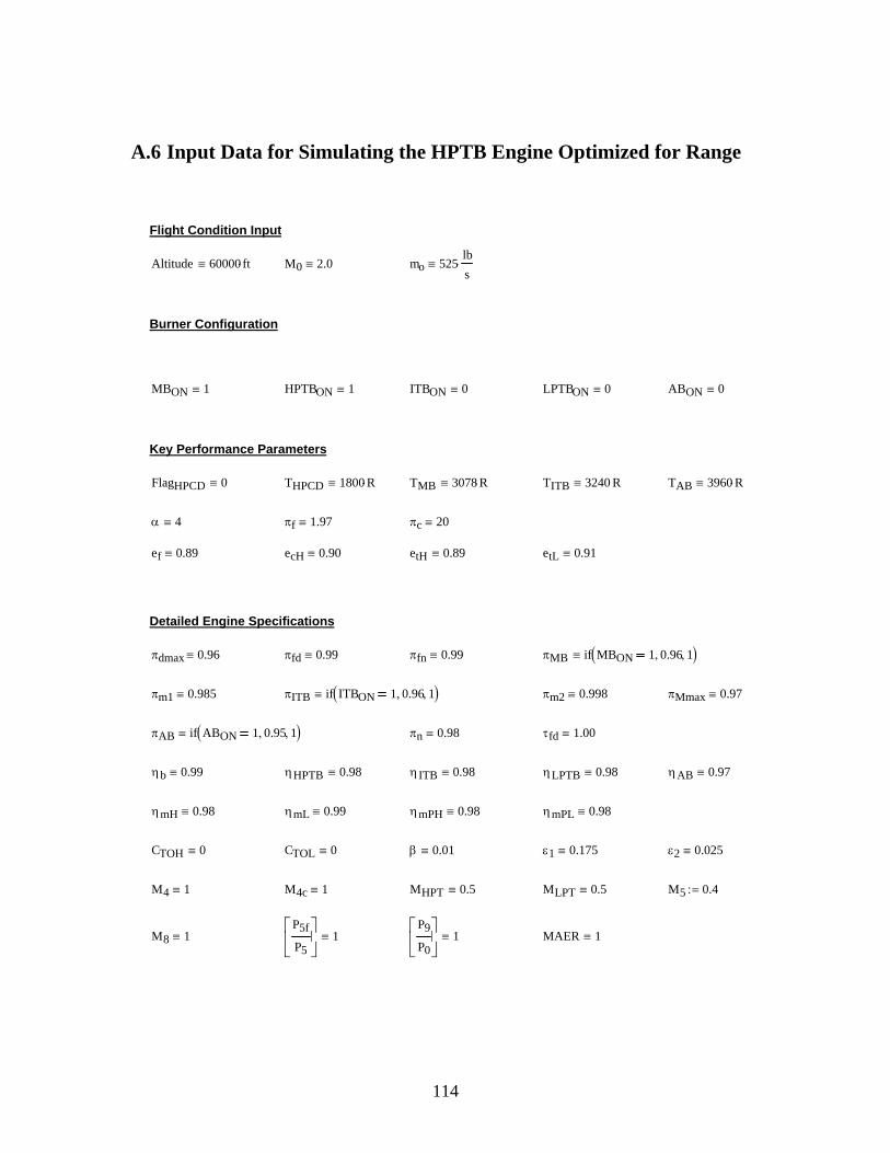
A.6 Input Data for Simulating the HPTB Engine Optimized for Range

πITB if ITBON 1 0.96, 1,( )≡ πm2 0.998≡ πMmax 0.97≡

πAB if ABON 1 0.95, 1,( )≡ πn 0.98≡ τfd 1.00≡

ηb 0.99≡ ηHPTB 0.98≡ ηITB 0.98≡ ηLPTB 0.98≡ ηAB 0.97≡

ηmH 0.98≡ ηmL 0.99≡ ηmPH 0.98≡ ηmPL 0.98≡

CTOH 0≡ CTOL 0≡ β 0.01≡ ε1 0.175≡ ε2 0.025≡

M4 1≡ M4c 1≡ MHPT 0.5≡ MLPT 0.5≡ M5 0.4:=

M8 1≡P5f

P5

⎡⎢⎣

⎤⎥⎦

1≡P9

P0

⎡⎢⎣

⎤⎥⎦

1≡ MAER 1≡

Flight Condition Input

Altitude 60000ft⋅≡ M0 2.0≡ mo 525lbs

⋅≡

Burner Configuration

MBON 1≡ HPTBON 1≡ ITBON 0≡ LPTBON 0≡ ABON 0≡

Key Performance Parameters

FlagHPCD 0≡ THPCD 1800 R⋅≡ TMB 3078 R⋅≡ TITB 3240 R⋅≡ TAB 3960 R⋅≡

α 4≡ πf 1.97≡ πc 20≡

ef 0.89≡ ecH 0.90≡ etH 0.89≡ etL 0.91≡

Detailed Engine Specifications

πdmax 0.96≡ πfd 0.99≡ πfn 0.99≡ πMB if MBON 1 0.96, 1,( )≡

πm1 0.985≡

114

A.7 Input Data for Simulating the HPTB Engine with Increased Cooling Optimized for Range

πITB if ITBON 1 0.96, 1,( )≡ πm2 0.987≡ πMmax 0.97≡

πAB if ABON 1 0.95, 1,( )≡ πn 0.98≡ τfd 1.00≡

ηb 0.99≡ ηHPTB 0.98≡ ηITB 0.98≡ ηLPTB 0.98≡ ηAB 0.97≡

ηmH 0.98≡ ηmL 0.99≡ ηmPH 0.98≡ ηmPL 0.98≡

CTOH 0≡ CTOL 0≡ β 0.01≡ ε1 0.19≡ ε2 0.16≡

M4 1≡ M4c 1≡ MHPT 0.5≡ MLPT 0.5≡ M5 0.4:=

M8 1≡P5f

P5

⎡⎢⎣

⎤⎥⎦

1≡P9

P0

⎡⎢⎣

⎤⎥⎦

1≡ MAER 1≡

Flight Condition Input

Altitude 60000ft⋅≡ M0 2.0≡ mo 525lbs

⋅≡

Burner Configuration

MBON 1≡ HPTBON 1≡ ITBON 0≡ LPTBON 0≡ ABON 0≡

Key Performance Parameters

FlagHPCD 0≡ THPCD 1800 R⋅≡ TMB 3078 R⋅≡ TITB 3240 R⋅≡ TAB 3960 R⋅≡

α 3.4≡ πf 1.88≡ πc 20≡

ef 0.89≡ ecH 0.90≡ etH 0.89≡ etL 0.91≡

Detailed Engine Specifications

πdmax 0.96≡ πfd 0.99≡ πfn 0.99≡ πMB if MBON 1 0.96, 1,( )≡

πm1 0.979≡

115

A.8 Input Data for Simulating the HPTB Engine Optimized for Size

πITB if ITBON 1 0.96, 1,( )≡ πm2 0.998≡ πMmax 0.97≡

πAB if ABON 1 0.95, 1,( )≡ πn 0.98≡ τfd 1.00≡

ηb 0.99≡ ηHPTB 0.98≡ ηITB 0.98≡ ηLPTB 0.98≡ ηAB 0.97≡

ηmH 0.98≡ ηmL 0.99≡ ηmPH 0.98≡ ηmPL 0.98≡

CTOH 0≡ CTOL 0≡ β 0.01≡ ε1 0.175≡ ε2 0.025≡

M4 1≡ M4c 1≡ MHPT 0.5≡ MLPT 0.5≡ M5 0.4:=

M8 1≡P5f

P5

⎡⎢⎣

⎤⎥⎦

1≡P9

P0

⎡⎢⎣

⎤⎥⎦

1≡ MAER 1≡

Flight Condition Input

Altitude 60000ft⋅≡ M0 2.0≡ mo 310lbs

⋅≡

Burner Configuration

MBON 1≡ HPTBON 1≡ ITBON 0≡ LPTBON 0≡ ABON 0≡

Key Performance Parameters

FlagHPCD 0≡ THPCD 1800 R⋅≡ TMB 3078 R⋅≡ TITB 3240 R⋅≡ TAB 3960 R⋅≡

α 1.7≡ πf 2.69≡ πc 20≡

ef 0.89≡ ecH 0.90≡ etH 0.89≡ etL 0.91≡

Detailed Engine Specifications

πdmax 0.96≡ πfd 0.99≡ πfn 0.99≡ πMB if MBON 1 0.96, 1,( )≡

πm1 0.985≡

116

A.9 Input Data for Simulating the HPTB Engine with Increased Cooling Optimized for Size

πITB if ITBON 1 0.96, 1,( )≡ πm2 0.987≡ πMmax 0.97≡

πAB if ABON 1 0.95, 1,( )≡ πn 0.98≡ τfd 1.00≡

ηb 0.99≡ ηHPTB 0.98≡ ηITB 0.98≡ ηLPTB 0.98≡ ηAB 0.97≡

ηmH 0.98≡ ηmL 0.99≡ ηmPH 0.98≡ ηmPL 0.98≡

CTOH 0≡ CTOL 0≡ β 0.01≡ ε1 0.19≡ ε2 0.16≡

M4 1≡ M4c 1≡ MHPT 0.5≡ MLPT 0.5≡ M5 0.4:=

M8 1≡P5f

P5

⎡⎢⎣

⎤⎥⎦

1≡P9

P0

⎡⎢⎣

⎤⎥⎦

1≡ MAER 1≡

Flight Condition Input

Altitude 60000ft⋅≡ M0 2.0≡ mo 349lbs

⋅≡

Burner Configuration

MBON 1≡ HPTBON 1≡ ITBON 0≡ LPTBON 0≡ ABON 0≡

Key Performance Parameters

FlagHPCD 0≡ THPCD 1800 R⋅≡ TMB 3078 R⋅≡ TITB 3240 R⋅≡ TAB 3960 R⋅≡

α 1.7≡ πf 2.44≡ πc 20≡

ef 0.89≡ ecH 0.90≡ etH 0.89≡ etL 0.91≡

Detailed Engine Specifications

πdmax 0.96≡ πfd 0.99≡ πfn 0.99≡ πMB if MBON 1 0.96, 1,( )≡

πm1 0.979≡

117

A.10 Input Data for Varying Cooling Flows in a Turburner

πITB if ITBON 1 0.96, 1,( )≡ πm2 0.998≡ πMmax 0.97≡

πAB if ABON 1 0.95, 1,( )≡ πn 0.98≡ τfd 1.00≡

ηb 0.99≡ ηHPTB 0.98≡ ηITB 0.98≡ ηLPTB 0.98≡ ηAB 0.97≡

ηmH 0.98≡ ηmL 0.99≡ ηmPH 0.98≡ ηmPL 0.98≡

CTOH 0≡ CTOL 0≡ β 0.01≡ ε1 0.175≡ ε2 0.025≡

M4 1≡ M4c 1≡ MHPT 0.5≡ MLPT 0.5≡ M5 0.4:=

M8 1≡P5f

P5

⎡⎢⎣

⎤⎥⎦

1≡P9

P0

⎡⎢⎣

⎤⎥⎦

1≡ MAER 1≡

Flight Condition Input

Altitude 60000ft⋅≡ M0 2.0≡ mo 1lbs

⋅≡

Burner Configuration

MBON 1≡ HPTBON 1≡ ITBON 0≡ LPTBON 0≡ ABON 0≡

Key Performance Parameters

FlagHPCD 0≡ THPCD 1800 R⋅≡ TMB 3078 R⋅≡ TITB 3240 R⋅≡ TAB 3960 R⋅≡

α 1≡ πf 3.91≡ πc 20≡

ef 0.89≡ ecH 0.90≡ etH 0.89≡ etL 0.91≡

Detailed Engine Specifications

πdmax 0.96≡ πfd 0.99≡ πfn 0.99≡ πMB if MBON 1 0.96, 1,( )≡

πm1 0.985≡

∗

∗ High-lighted parameters (in yellow) are varied during the calculations.

118

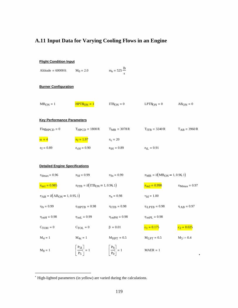
A.11 Input Data for Varying Cooling Flows in an Engine

πITB if ITBON 1 0.96, 1,( )≡ πm2 0.998≡ πMmax 0.97≡

πAB if ABON 1 0.95, 1,( )≡ πn 0.98≡ τfd 1.00≡

ηb 0.99≡ ηHPTB 0.98≡ ηITB 0.98≡ ηLPTB 0.98≡ ηAB 0.97≡

ηmH 0.98≡ ηmL 0.99≡ ηmPH 0.98≡ ηmPL 0.98≡

CTOH 0≡ CTOL 0≡ β 0.01≡ ε1 0.175≡ ε2 0.025≡

M4 1≡ M4c 1≡ MHPT 0.5≡ MLPT 0.5≡ M5 0.4:=

M8 1≡P5f

P5

⎡⎢⎣

⎤⎥⎦

1≡P9

P0

⎡⎢⎣

⎤⎥⎦

1≡ MAER 1≡

Flight Condition Input

Altitude 60000ft⋅≡ M0 2.0≡ mo 525lbs

⋅≡

Burner Configuration

MBON 1≡ HPTBON 1≡ ITBON 0≡ LPTBON 0≡ ABON 0≡

Key Performance Parameters

FlagHPCD 0≡ THPCD 1800 R⋅≡ TMB 3078 R⋅≡ TITB 3240 R⋅≡ TAB 3960 R⋅≡

α 4≡ πf 1.97≡ πc 20≡

ef 0.89≡ ecH 0.90≡ etH 0.89≡ etL 0.91≡

Detailed Engine Specifications

πdmax 0.96≡ πfd 0.99≡ πfn 0.99≡ πMB if MBON 1 0.96, 1,( )≡

πm1 0.985≡

∗

∗ High-lighted parameters (in yellow) are varied during the calculations.

119

Appendix B Engine Data Used for Validation Tests

The experimental engine data used in this research to validate the program developed are excerpted from the excellent work by St. Peter [31]. St. Peter extracted the actual engine data from various sources, mainly the Department of Defense, to complement his work on recounting the development of gas turbine engines in the United States. His book is highly inspirational to this author and provides insight into various developmental challenges of a gas turbine engine. This author highly recommends St. Peter’s book to the reader of this dissertation.

For ease of references, the engine data of F101 and TF34, used in this research for validation, are actually scanned and provided here. These data are shown in the next three pages, in the order of the disclaimer of data source, the data for F101, and then the data for TF34.

120

121

122

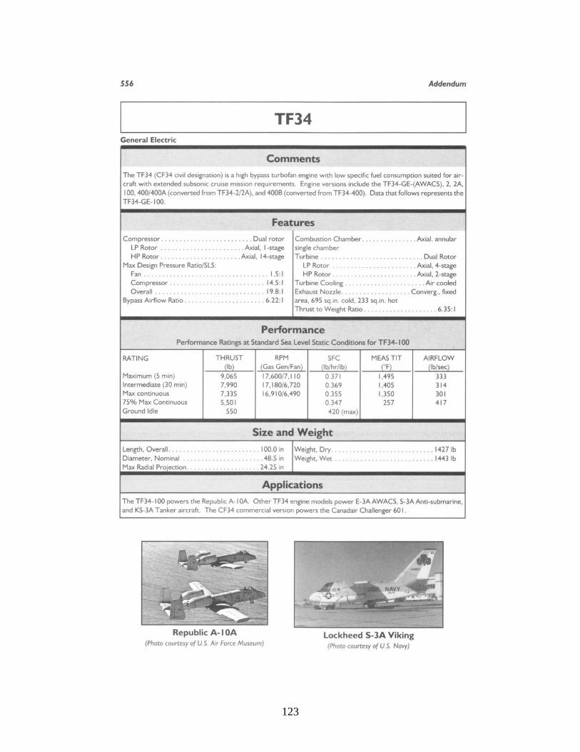
123

References

[1] Jane’s Information Group, Jane’s All-the-World’s Aircraft 2003-2004, Jane’s Information Group, Alexandria, VA, 2004.

[2] Jane’s Information Group, Jane’s Aero-Engines, Issue 9, Jane’s Information Group, Alexandria, VA, 2001.

[3] Bradley, M., et al., “Revolutionary Turbine Accelerator (RTA) Two-Stage-To-Orbit (TSTO) Vehicle Study”, 38th AIAA/ASME/SAE/ASEE Joint Propulsion Conference & Exhibit, Indianapolis, IN, AIAA-2002-3902, 2002.

[4] Ramohalli, K. N. R., “Isothermal Combustion for Improved Efficiencies”, 23rd AIAA/SAE/ASME/ASEE Joint Propulsion Conference, San Diego, CA, AIAA-87-1999, 1987.

[5] Sirignano, W. A., Delplanque, J. P., and Liu, F., “Selected Challenges in Jet and Rocket Engine Combustion Research”, 33rd AIAA/ASME/SAE/ASEE Joint Propulsion Conference & Exhibit, Seattle, WA, AIAA-97-2701, 1997.

[6] Liu, F. and Sirignano, W. A., “Turbojet and Turbofan Engine Performance Increases through Turbine Burners”, 38th Aerospace Sciences Meeting & Exhibit, Reno, NV, AIAA-2000-0741, 2000.

[7] Hill, Philip G., and Peterson, Carl R., Mechanics and Thermodynamics of Propulsion, 2nd Edition, Addison-Wesley Publishing Company, 1992.

[8] Andriani, R., et al., “Design Proposals for Constant Temperature Turbine Engine for Propulsion System”, 37th AIAA/ASME/SAE/ASEE Joint Propulsion Conference & Exhibit, Salt Lake City, UT, AIAA-2001-3750, 2001.

[9] Andriani, R. and Ghezzi, U., “Off-Design Analysis of Constant Temperature Turbine Jet Engine”, 38th AIAA/ASME/SAE/ASEE Joint Propulsion Conference & Exhibit, Indianapolis, IN, AIAA-2002-3766, 2002.

[10] Fang, X., Liu, F., and Sirignano, W. A., “Ignition and Flame Studies for an Accelerating Transonic Mixing Layer”, 38th Aerospace Sciences Meeting & Exhibit, Reno, NV, AIAA-2000-0437, 2000.

[11] Cai, J., Icoz, O., Liu, F., and Sirignano, W. A., “Ignition and Flame Studies for Turbulent Transonic Mixing in a Curved Duct Flow”, 39th AIAA Aerospace Sciences Meeting & Exhibit, Reno, NV, AIAA-2001-0189, 2001.

124

[12] Nagumo, T., Toda, K., and Yamamoto, M., “Three-Dimensional Computations of Hydrogen-Fueled Combustion within Turbine Blade Passage”, 39th AIAA Aerospace Sciences Meeting & Exhibit, Reno, NV, AIAA-2001-0632, 2001.

[13] Isvoranu, Dragos D., and Cizmas, Paul G. A., “Numerical Simulation of Combustion and Rotor-Stator Interaction in a Turbine Combustor”, International Journal of Rotating Machinery, 9, pp. 363-374, 2003.

[14] Rice, Matthew J., Simulation of Isothermal Combustion in Gas Turbines, Master of Sciences Thesis, 2004

[15] Siow, Y. K. and Yang, S. L., “Numerical Study and Design of Interstage Turbine Burner”, 38th AIAA/ASME/SAE/ASEE Joint Propulsion Conference & Exhibit, Indianapolis, IN, AIAA-2002-3727, 2002.

[16] Liew, K. H., et al., “A Complete Parametric Cycle Analysis of a Turbofan with Interstage Turbine Burner”, 41st AIAA Aerospace Sciences Meeting & Exhibit, Reno, NV, AIAA-2003-0685, 2003.

[17] Lewis, G. D., “Centrifugal-Force Effects on Combustion”, 14th Symposium (International) on Combustion, the Combustion Institute, pp. 413-419, 1973.

[18] Chomiak, J., “Dissipation Fluctuations and the Structure and Propagation of Turbulent Flames in Premixed Gases at High Reynolds Numbers”, 16th Symposium (International) on Combustion, The Combustion Institute, pp. 1665-1673, 1977.

[19] Yonezawa, Y., Toh, H., Goto, S., and Obata, M., “Development of the Jet-Swirl High Loading Combustor”, 26th AIAA/SAE/ASME/ASEE Joint Propulsion Conference, Orlando, FL, AIAA-90-2451, 1990.

[20] Sturgess, G. J., et al., “Ultra-Compact Combustion Technology Using High Swirl for Enhanced Burning Rate”, 38th AIAA/ASME/SAE/ASEE Joint Propulsion Conference & Exhibit, Indianapolis, IN, AIAA-2002-3725, 2002.

[21] Papamoschou, D. and Debiasi, M., “Conceptual Development of Quiet Turbofan Engines for Supersonic Aircraft”, Journal of Propulsion and Power, Vol. 19, No. 2, pp. 161-169, 2003

[22] McBride, B. J., Gordon, S., and Reno, A., “Coefficients for Calculating Thermodynamic and Transport Properties of Individual Species”, NASA-TM-4513, National Aeronautics and Space Administration, 1993.

[23] Coordinating Research Council, Inc., Handbook of Aviation Fuel Properties, Society of Automotive Engineers, Inc., 1984.

[24] Mattingly, Jack D., Heiser, William H., and Daley, Daniel H., Aircraft Engine Design, American Institute of Aeronautics and Astronautics, Inc., 1987.

125

[25] U.S. Department of Defense, “Model Specification for Engines, Aircraft, Turbojet”, Military Specification MIL-E-5008B, Washington, DC, Jan. 1959.

[26] Oates, G. C., The Aerothermodynamics of Gas Turbine and Rocket Propulsion, 3rd ed., American Institute of Aeronautics and Astronautics, Inc., 1997.

[27] Oates, G. C., “Performance Estimation for Turbofans with and without Mixers”, Journal of Propulsion and Power, Vol. 1, No. 3, pp. 252-256, 1985.

[28] Walsh, P. P. and Fletcher, P., Gas Turbine Performance, Blackwell Science Ltd and American Society of Mechanical Engineers, 1998.

[29] Pearson, H., “Mixing of Exhaust and Bypass Flow in a Bypass Engine”, Journal of Royal Aeronautical Society, 66, p. 528, 1962.

[30] Frost, T. H., “Practical Bypass Mixing Systems for Fan Jet Aero-Engines”, The Aeronautical Quarterly, May, pp. 141-160, 1966.

[31] St. Peter, James, The History of Aircraft Gas Turbine Engine Development in the United States…A Traditional of Excellence, International Gas Turbine Institute of the American Society of Mechanical Engineers, 1999.

[32] Lowrie, B. W., Denning, R. M., and Gupta, P. C., “The Next Generation Supersonic Transport Engine Critical Issues”, PNR90576, Rolls Royce plc, 1989.

[33] Rech, J. and Leyman, C. S., A Case Study by Aerospatiale and British Aerospace on the Concorde, Institute of Aeronautics and Astronautics, Inc., 1980.

[34] Horlock, J. H., Watson, D. T., and Jones, T. V., “Limitations on Gas Turbine Performance Imposed by Large Turbine Cooling Flows”, Journal of Engineering for Gas Turbine and Power, Vol. 123, pp. 487-494, 2001.

126

Vita

The author, Ya-Tien “Mac” Chiu, was born in Taipei, Taiwan on November 5, 1973. He grew up in the same city and entered the National Tsing-Hua University located in Hsin-chu in 1991. After obtaining his Bachelor of Science degree in Mechanical Engineering in 1995, he served in the Republic of China Air Force as an Air Traffic Controller for the next two years. In August 1997, he first came to United States in pursuit of advanced education at Virginia Polytechnic Institute & State University. He performed CFD simulations for the Navy Air Warfare Center for his Master of Science degree during 1998 and 1999. After obtaining his master degree, he continued toward the degree of Doctor of Philosophy till 2004 with research presented in this dissertation. He also acted as instructors as well as teaching assistants to improve his communication skills and to further his skills in teaching. After graduation, he expects to work as a research scientist in the turbomachinery industry.

127