A Parallel Lanczos Methodfor Symmetric Generalized Eigenvalue ProblemsyKesheng Wuzand Horst SimonzDecember, 1997AbstractLanczos algorithm is a very e�ective method for �nding extreme eigenvalues ofsymmetric matrices. It requires less arithmetic operations than similar algorithms,such as, the Arnoldi method. In this paper, we present our parallel version of theLanczos method for symmetric generalized eigenvalue problem, PLANSO. PLANSO isbased on a sequential package called LANSO which implements the Lanczos algorithmwith partial re-orthogonalization. It is portable to all parallel machines that supportMPI and easy to interface with most parallel computing packages. Through numericalexperiments, we demonstrate that it achieves similar parallel e�ciency as PARPACK,but uses considerably less time.The Lanczos algorithm is one of the most commonly used methods for �nding extremeeigenvalues of large sparse symmetric matrices [2, 3, 13, 15]. A number of sequential imple-mentations of this algorithm are freely available from various sources, for example, NETLIB(http://www.netlib.org/) and ACM TOMS (http://www.acm.org/toms/). These pro-grams have been successfully used in many scienti�c and engineering applications. However,a robust parallel Lanczos code is still missing. At this time, 1997, the only widely availableparallel package for large eigenvalue problems is PARPACK1, which implements the implic-itly restarted Arnoldi algorithm. The Arnoldi algorithm and the Lanczos algorithm can beapplied to many forms of eigenvalue problems. Applied on symmetric eigenvalue problems,these two algorithms are mathematically equivalent. However, the Lanczos algorithm ex-plicitly takes advantage of the symmetry of the matrix, and uses signi�cantly less arithmeticoperations than the Arnoldi algorithm. Thus, it is worthwhile to implement the Lanczosalgorithm for symmetric eigenvalue problems.yThis work was supported by the Director, O�ce of Energy Research, O�ce of Laboratory Policy andInfrastructure Management, of the U.S. Department of Energy under Contract No. DE-AC03-76SF00098.zLawrence Berkeley National Laboratory, NERSC, Berkeley, CA 94720. Email addresses: fkewu,simong-@nersc.gov.1PARPACK is a parallel version of ARPACK which implements a implicit restarted Arnoldi algorithm.The source code is available at http://www.caam.rice.edu/�kristyn/parpack home.html. Its sequentialcounterpart is documented in [18]. 1

LBNL-41284

Since there are a number of sequential implementations of the Lanczos algorithm, we de-cided to build our parallel Lanczos code based on an existing package. The major di�erencesbetween di�erent implementations of the symmetric Lanczos algorithm include: whetherand how to perform re-orthogonalization, whether to solve the generalized eigenvalue prob-lem, where to store the Lanczos vectors, what block size to use, and so on. The choiceon re-orthogonalization can have major impact on most aspects of the program. If no re-orthogonalization is performed, the Lanczos vectors may lose orthogonality after a numberof steps. In this case, the computed eigenvalues may have extra multiplicities. These extraeigenvalues are known as spurious eigenvalues. Identifying and eliminating spurious eigen-values may be a signi�cant amount of work. The time spent in computing the spuriouseigenvalues could potentially be used to compute other eigenvalues. The main advantageof not performing re-orthogonalization is that it can be implemented with a very smallamount of computer memory, since only two previous Lanczos vectors need to be saved[3, 4, 19, 20]. However, on many parallel computers, memory is not a limiting factor forthe majority of applications. For these applications, it is appropriate to save all Lanczosvectors, perform re-orthogonalization and eliminate the spurious eigenvalues. Among thevarious re-orthogonalization techniques [3, 12, 13, 17], it was shown that the !-recurrencecan predict the loss of orthogonality better than others, such as selective re-orthogonalization[17]. Given the same tolerance on orthogonality, partial re-orthogonalization scheme, whichuses !-recurrence, performs less re-orthogonalization. In [17], it was also shown that theLanczos algorithm can produce correct eigenvalues with the loss of orthogonality as largeas p�, where � is the unit round-o� error. The sequential Lanczos package we have chosento use, LANSO, implements the !-recurrence and performs re-orthogonalization only whenloss of orthogonality is larger than p�. This scheme reduces the re-orthogonalization to theminimal amount without sacri�cing the reliability of the solutions.The LANSO package was designed to solve symmetric generalized eigenvalue problems.It is more exible than a package that was designed just for symmetric simple eigenvalueproblems. It also lets users choose their own schemes of storing the Lanczos vectors. Thesecharacteristics make it a very good starting point to build a parallel Lanczos algorithm. Thebulk of this paper is devoted to evaluating the performance of our parallel Lanczos codeand comparing it with existing parallel eigenvalue code. We are also interested in de�ningpossible enhancements to the parallel Lanczos method by analyzing the overall performancerelative to its major components. For example, LANSO only expands the basis one vector ata time, while a block version could be more e�cient on parallel machines. The third goal ofthis paper is to evaluate the performance of the Lanczos code on di�erent parallel platforms.Two di�erent platforms, a tight-coupled MPP and cluster of SMPs, are used. MPP systemsare currently the most e�ective high performance computing systems. Clusters of SMPs arelow cost alternatives to the MPP systems. We want to ensure that our program is e�cienton both platforms.Given a sequential version of the Lanczos code, there are many ways to develop a parallelcode from it. The approach taken here turns the sequential code into a Single-Program-Multiple-Data (SPMD) program. The converted program can easily interface with mostexisting parallel sparse matrix packages such as AZTEC [10], BLOCKSOLVE [11], PETSc2

[1], P SPARSLIB2, and so on. The details on porting LANSO are discussed in section1 of this report. Section 2 describes how to use the parallel LANSO program, and theperformance of a few examples are shown in section 3 and 4. Section 3 shows the resultsfrom a massively parallel machine (MPP) and section 4 shows the results from a clusterof symmetric multiprocessors (SMP). A short summary is provided following the testingresults. The user interface of PLANSO is documented in the appendix of this report.Algorithm 1 Symmetric Lanczos iterations starting with a user-supplied starting vectorr0.1. Initialization. �0 = kr0k, q0 = 0.2. Iterate. For i = 1; 2; : : :,(a) qi = ri�1=�i�1,(b) p = Aqi,(c) �i = qTi p,(d) ri = p� �iqi � �i�1qi�1,(e) �i = krik.1 Parallelizing LANSOThe Lanczos algorithm for symmetric matrices, see algorithm 1, can be found in manystandard textbooks, e.g., [7, section 9.1.2], [13], and [16, section 6.6]. In this algorithm, themain operations are matrix-vector multiplication, SAXPY, dot-product, and computing the2-norm of r. The above algorithm builds an orthogonal basis Qi = [q1; : : : ; qi] and computesa tridiagonal matrix Ti as follows,Ti � QTi AQi = 0BBBBBBB@ �1 �1�1 �2 �2. . . . . . . . .�i�2 �i�1 �i�1�i�1 �i1CCCCCCCA :After any i steps of the Lanczos algorithm, the Rayleigh-Ritz projection can be used toextract an approximate solution to the original eigenvalue problem. Let (�; y) be an eigen-pair of Ti, i.e., Tiy = �y, then � is an approximate eigenvalue or a Ritz value of A, thecorresponding approximate eigenvector or Ritz vector is x = Qiy. In the Lanczos eigenvaluemethod, the accuracy of this approximate solution is known without explicitly computing theeigenvector x. Thus, we only need to compute x after we have found all desired eigenpairs.In practice, the Lanczos vectors may lose orthogonality when the above algorithm in carriedout in oating-point arithmetic. Occasionally, the Gram-Schmidt procedure is invoked to2The latest P SPARSLIB source code is available at http://www.cs.umn.edu/�saad/.3

explicitly orthogonalize a residual vector against all previous Lanczos vectors. The Gram-Schmidt procedure can be broken up into a series of dot-product and SAXPY operations.However, we will not break it down because it can be implemented more e�ciently than call-ing dot-product and SAXPY functions. All in all, the major computation steps in a Lanczosalgorithm are: matrix-vector multiplication, SAXPY, dot-product, norm computation, re-orthogonalization, solving the small eigenvalue problem, and computing the eigenvectors. Inmost cases, the oating-point operations involved in solving the small eigenvalue problem arenegligible compared to the rest of the algorithm. We replicate the operation of solving thissmall eigenvalue problem on each processor to simplify the task of parallelizing the Lanczosalgorithm.Algorithm 2 Lanczos iterations for generalized eigenvalue problem Kx = �Mx.1. Initialization. �0 = qrT0Mr0, q0 = 0.2. Iterate. For i = 1; 2; : : :,(a) qi = ri�1=�i�1,(b) p = M�1Kqi,(c) �i = qTi Mp,(d) ri = p� �iqi � �i�1qi�1,(e) �i = qrTi Mri.The eigenvalue package LANSO is maintained by professor Beresford Parlett of theUniversity of California at Berkeley. It implements the Lanczos algorithm with partialre-orthogonalization for symmetric generalized eigenvalue problem, Kx = �Mx, see Algo-rithm 2 [13]. The LANSO code does not directly access the sparse matrices involved in theeigenvalue problem, instead, it requires the user to provide routines with prescribed interfaceto perform the matrix-vector multiplications. This greatly simpli�es the work needed to par-allelize LANSO, since all operations to be parallelized are dense linear algebra operations.The communication operations required by these dense linear algebra functions are limited.This allows us to use any of the common communication libraries. In fact, all operationsthat require communication can be constructed as a series of inner-product options whichcan be implemented with only one global sum operation that adds up one number from eachPE and returns the result to all. Since many of the sparse linear algebra packages use MPIto exchange data, we have chosen to follow the precedence and use MPI as well.The dense linear algebra operations involved in the Lanczos iterations, dot-product,SAXPY and orthogonalization operations, can be e�ectively parallelized if the Lanczos vec-tors are uniformly and conformally mapped onto all PEs. In other words, if the matrixsize is n � n and p PEs are used, the same n=p elements of each Lanczos vector will resideon one PE. In this case, the SAXPY operation is perfectly parallel. So is the operation ofcomputing Ritz vectors after the small eigenvalue problem is solved. As long as the vectorsare conformally mapped and no element resides on more than one processor, a dot-productcan be computed with a local dot-product operation followed a global sum operation. When4

there are an equal number of elements on each processor, these parallel operations haveperfect load-balance.Since the LANSO package requires the user to provide matrix-vector multiplication rou-tines, the data mapping should allow the user to easily interface with other packages touse their matrix-vector multiplication routines or linear system solution routines. Manyof the sparse matrix packages for parallel machines have matrix-vector multiplication andlinear system solution routines which produce output vectors that are conformal to the in-put vectors, for example, AZTEC, BLOCKSOLVE, P SPARSLIB, PETSc. Thus, requiringthe Lanczos vectors to be mapped conformally makes the parallel Lanczos routine easy tointerface the parallel LANSO code with these packages.Using MPI, the parallel dot-product routine can be constructed by computing the partialsum on each PE and adding up the partial sums using MPI ALLREDUCE function. Whencomputing norm of a vector, one can scale the vector �rst so that its largest absolute valueis one. This increases the reliability of the norm computing routine. On distributed envi-ronments, this means that an extra global reduction is required to �nd the largest absolutevalue of the array and at least twice the oating-point multiplications are required comparedto the case without scaling. In the regular Lanczos algorithm, we need to compute the normof the following vectors: the initial guess, a random vector, or the result of matrix-vectormultiplication. Random vectors generated in LANSO have values in between -1 and 1. Thenorms of vectors generated in the matrix-vector multiplications are limited by the norm ofthe matrix, since the input vectors to matrix-vector multiplications are always normalized.The only possible source of badly scaled vector is the user-supplied initial guess. Since aneigenvector should be unitary, we expect the user to provide an initial guess that is wellscaled. If the user-supplied initial guess is badly scaled, i.e., the sum of the square of theelements is too large for the oating-point representation, a random vector is used as theinitial guess. Thus, if the norm of the operator (A, M�1K, or (K � �M)�1M) is not verylarge, say less than 10100 when the Lanczos vectors are stored as 64-bit IEEE oating-pointnumbers, there is no bene�t in scaling the vector when computing its norm. There is a slightchance that a shift-and-invert operator may have an exceedingly large norm. However, thisspecial case probably deserves separate treatment. Therefore we have decided not to performscaling when computing the norm of a vector.When the Lanczos routine has detected an invariant subspace, and still more eigenvaluesare wanted, it will continue with a random vector. We do not anticipate that the randomvectors are needed frequently, nor do we anticipate that the quality of the random numbergeneration will dominate the overall solution time. Thus we are satis�ed with the simplerandom number generator used in LANSO. The only change made is to have each PE generatea di�erent seed before the random number generator is used.In our current implementation, the small eigenvalue problem is replicated on each PE.The size of the small eigenvalue problem is equal to the number of Lanczos steps taken. Ifthe number of Lanczos steps required to solve the given eigenvalue problem is small, thanreplicating it is an acceptable option. If the number of steps is large, it might be moree�cient to let the processors solve this problem in collaboration. We believe the number ofLanczos steps will be relatively small in most cases, so we have chosen not to parallelize theoperation at this time. 5

For most of the dense linear algebra operations, LANSO only needs to know the localproblem size, i.e., the number of elements of a Lanczos vector on the current processor.There are two operations where the global problem size is needed. One, when computing theestimate of loss of orthogonality, we need to use �pn where n must be the global problemsize. The other use of global problem size is to ensure the maximum number of Lanczossteps do not exceed the global problem size.When converting LANSO to a parallel program, we also need to change how the programprints diagnostic messages. Most of the messages would be the same if printed from di�erentprocessors. In this case, only processor 0 will print them. If di�erent PE will print di�erentmessages, they will be printed with the PE number associated with the message.Overall, a fairly small number of changes are required to parallelize LANSO. Our ex-perience is representative of many parallelization e�orts involving Krylov-based projectionmethods for linear systems and eigenvalue problems [10, 11, 14].2 Using the parallel LANSOThe details of the user interface are described in the appendix of this report. Another goodsource of information is the documentation that comes with the source code. Here we providea brief introduction to basic elements needed in order to use the parallel LANSO code. Touse the program, the user should provide the following functions.1. The operator of the eigenvalue problem, OP and OPM. To solve a standard symmetriceigenvalue problem, Ax = �x, the function OP performs the matrix-vector multiplica-tion with A, the function OPM should simply copy its input vector to the output vector.To solve a symmetric generalized eigenvalue problem, Kx = �Mx, the function OPMshould be a matrix-vector multiplication routine that multiplies M , the function OPshould perform the matrix-vector multiplication with the matrix either in the standardform, M�1K, or the shift-and-invert form, (K � �M)�1M . As mentioned before, thematrix-vector multiplication routines should map the input and output vectors con-formally, i.e., if the ith (global index) element of the input vector is on processor j,the ith element of the output vector should be also on processor j. The local indexof ith element on processor j should be the same for both input and output vectors.The conformal mapping is used by most existing parallel sparse matrix computationpackages, e.g., AZTEC, BLOCKSOLVE, P SPARSLIB, PETSc.Allowing a user-supplied matrix-vector multiplication routine to be used makes it pos-sible for a user to select di�erent schemes to store the matrix and to use their favoritelinear system solver in the generalized eigenvalue case. For most applications, thereis usually a more speci�c sparse matrix storage format that is more convenient forthat particular application. On parallel machines, there is usually a custom parallelmatrix-vector multiplication that is e�cient for the particular application as well. Nooperations inside PLANSO depend on the global index of a vector element, thus as longas the matrix vector multiplications produce output that are conformal to the inputvector, PLANSO can function correctly and �nd the appropriate eigenvalues and theircorresponding eigenvectors. 6

2. A function to access Lanczos vectors, STORE. It is used by the program to store theLanczos vectors no longer needed for regular steps of Lanczos algorithm, see Algo-rithm 2. The Lanczos vectors may be needed again to compute the Ritz vectors orto perform re-orthogonalization. The users have the exibility of either storing theLanczos vectors in-core or out-of-core by simply modifying this single function.3. A parallel orthogonalization routine PPURGE. The user may decide whether or not toreplace this routine. It performs re-orthogonalization when the loss of orthogonalityhas become severe. The user may replace it to enhance the performance of the defaultre-orthogonalization procedure which performs the modi�ed Gram-Schmidt procedureand retrieves the old Lanczos vectors one after the other. A series of global sumoperations are needed to compute the dot-products between the old Lanczos vectorsand the new one. If the Lanczos vectors are stored in-core, the classic Gram-Schmidtprocedure is usually more e�cient on parallel machines. A version of PPURGE thatimplements the classic Gram-Schmidt procedure is presented with every example thatstores the Lanczos vectors in-core. Should the user decide to have a customized PPURGEfunction, the examples can be used as starting points.The size of workspace required by the parallel LANSO on each PE is completely de�nedby the local problem size and the maximum number of Lanczos steps allowed. If the localproblem size is Nloc and the maximum number of Lanczos steps desired is LANMAX, theworkspace size needs to be at least 5 � Nloc + 4 � LANMAX + max(Nloc; LANMAX + 1) + 1. Ifeigenvectors are needed, additional LANMAX� LANMAX elements are needed.With PLANSO, the user may choose to compute a few extreme eigenvalues from bothends of the spectrum or one end of the spectrum. The eigenvalue routine will stop when thedesired number of eigenvalues are found or the maximum allowed number of Lanczos stepsis reached. After the program returns, the approximate eigenvalues and their correspondingerror estimates are returned to the caller. The approximate eigenvectors may be written to a�le or the user may choose to compute the approximate eigenvectors outside of the LANSOprogram using the Lanczos vectors.3 Performance on MPPThis section demonstrates the e�ectiveness of the parallel LANSO code by examples. Inorder for a parallel program to be usable in a massively parallel environment like Cray T3E,it is important that the algorithm is scalable. There are two generally accepted approachesto measure scalability. One �xes the global problem size and the other �xes the local problemsize on each PE. In this section we will show both types of test cases.At the time of this test, the Cray T3E used was using operating system UNICOS/mkversion 1.5. The Fortran compiler was CF90 version 3.0. The C compiler was Cray's Ccompiler Version 6.0. The Fortran programs are compiled with aggressive optimization ag-Oaggress,scalar3,unroll2. The C functions are compiled with standard optimization ag -O. The peak oating-point operation rate was 900 MFLOPS, and the peak data ratewas 7200MB/sec for loading data from cache and 3600MB/sec for storing to cache.7

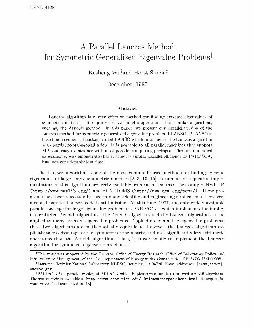
For �xed global problem size test cases, we have chosen to �nd the eigenvalues of twolarge sparse matrices in Harwell-Boeing format [6]. The �rst matrix is a structural model of aspace shuttle rocket booster from NASA Langley called NASASRB. It has 54,870 rows and2,677,324 nonzero elements. The matrix is stored in Harwell-Boeing format which storesonly half of the nonzero elements. The �le size is about 36MB. The second test matrixis CPC sti�ness matrix (CPC.K). It has 637,244 rows and 30,817,002 nonzero elements.The �le size is about 600MB. The matrix CPC.K is reordered using reverse Cuthill-McKeeordering before it was used in our tests. The reverse Cuthill-Mckee ordering is one of thecommon ordering schemes used to reduce the bandwidth of a sparse matrix [5]. It is ageneric algorithm to reduce the data communication required during sparse matrix-vectormultiplication. We did not use better reordering schemes because the reordered matricesshow reasonable performance in the tests. In addition, we only need the performance of thematrix-vector multiplication as a reference to measure the overall performance of PLANSO.3.1 Fixed size testsThe �rst test performed is to see scalability of the major components of the LANSO program.Figure 1 shows the oating-point performance per PE of matrix-vector multiplication, dot-product, SAXPY and orthogonalization. They are not directly measured from the LANSOroutine, but the test uses the same matrices and same size vectors as in LANSO. Theperformance of the orthogonalization is measured from orthogonalizing one vector against32 orthonormal vectors. Given the maximum data rate, the peak rate for SAXPY on 8-byte oating-point arrays is 450MFLOPS. We are able to achieve almost 85% of this peak ratewhen the arrays can �t into cache. The dot-product operation and norm computation have apeak rate of 900MFLOPS, but the best measured rate is about 11% of this peak rate. Thereare two main reasons for this. One is that the global reduction takes signi�cant amountof time in dot-product operation. The other reason is that most of the time the data isloaded from main memory which has a much slower rate than 3600MB/sec. The parallele�ciency for dot-product operation is the lowest among all major components of PLANSO.For the NASASRB test problem, the oating-point operation rate of dot-product operationand 2-norm computation on 32-PE partition is only about 40% of the rate on 1 PE. Whenmore PE is used, the performance degradation of dot-product is even more pronounced. Inthe CPC.K example, the performance of dot-product on 512 PE is only 25% of that of 16-PEcase.The e�ciencies shown in Figure 1 are measured as follows. In the NASASRB case, thee�ciency of using p-PE is the ratio of the performance on p-PE versus that of the 1-PE case.For example, the speed of the matrix-vector operation is 51.6MFLOPS per PE on 16 PEs,and 64.1MFLOPS on 1 PE. Thus the e�ciency of the matrix-vector operation on 16-PE is80%. The e�ciency of the CPC.K example is measured against the performance of 16-PEcase. The speed of the matrix-vector multiplication is 35.8MFLOPS per PE on 512 PEs and57.5 on 16-PE. Thus, the e�ciency of multiplying CPC.K on 512 PE is 62%.The orthogonalization operations run at about the same rate on di�erent size partitions.The performance of the orthogonalization procedure could be di�erent if the number oforthonormal vectors is di�erent. Typically, the performance increases as the number of8

1 2 4 8 16 320

100

200

300

400

Number of PEs

MF

LO

PS

pe

r P

E

MATVEC

Dot−product

2−NORM

SAXPY

ORTHO

1 2 4 8 16 320

0.2

0.4

0.6

0.8

1

Number of PEs

Eff

icie

ncy

NASASRB

MATVEC Dot−productORTHO

16 32 64 128 256 5120

100

200

300

400

Number of PEs

MF

LO

PS

pe

r P

E

MATVEC

Dot−product

2−NORM

SAXPY

ORTHO

16 32 64 128 256 5120

0.2

0.4

0.6

0.8

1

Number of PEs

Eff

icie

ncy

CPC.K

MATVEC Dot−productORTHO

Figure 1: Scalability of core operations of PLANSO on T3E with �xed global problem size.

9

orthonormal vectors increases. In the case tested, the number of orthonormal vectors is32. In many cases, the �rst re-orthogonalization occurs after forty or �fty steps of Lanczositerations. The performance of the orthogonalization operation measured could be regardedas typical. In both NASASRB and CPC.K cases the per PE performance of orthogonalizationoperation is fairly constant as the number of PE changes. Its oating-point operation rateis much higher than most other operations.The bulk of the oating-point operations of algorithm 1 is in applying the operator (A,M�1K, or (K � �M)�1M). LANSO routine requires the user to supply this operation. Thematrix-vector multiplication routine we use in this test is from the P SPARSLIB. It does athorough job of analyzing the communication pattern and only passes the minimum amountof data among the processors. It also takes advantage of MPI persistent communicationrequest and overlaps the communication and computation inside the matrix-vector multipli-cation routine. The intention of this test is to provide a reference point to measure how wellthe parallel LANSO works. The exact performance of matrix-vector multiplications, whichcould be highly problem-dependent, is not the main interest of this paper.On 1-PE, the sparse matrix-vector multiplication with NASASRB runs at about 64MFLOPS. The e�ciency of matrix-vector multiplication with NASASRB is above 80% whenless than 16 PEs are used. When the matrix is mapped onto 32 PEs, the distributed matrix-vector multiplication routine runs at about 38MFLOPS per PE which is nearly 60% of thesingle PE performance. This signi�cant performance decrease from 16-PE case to 32-PEcase can be partly explained by the di�erence in communication versus computation ratio.In both 16-PE and 32-PE cases, the number of bytes exchanged during matrix-vector mul-tiplication is about the same, however the amount of oating-point operation is essentiallyreduced by half on each PE. More importantly, the part of the arithmetic operation thatcan be overlapped with communication reduced very signi�cantly from 16-PE case to 32-PEcase. The communication latency can no longer be e�ectively hidden in 32-PE case.The e�ciency of the matrix-vector multiplication with CPC.K is better than 80% whenpartition size is less than 128. Going from a 128-PE partition to a 256-PE partition, the num-ber of neighbors a PE sends messages to changes from 4 to 8. This increases the likelihood ofcongestion during communication which slows down the communication. In addition, thereare a signi�cant number of PEs where there is very little overlapping between communicationand computation because of the decrease in the amount of arithmetic operations on eachPE. The e�ciency of the matrix-vector multiplication with CPC.K is about 60% on 256 PEand 512 PE of T3E. The e�ciency on 512-PE partition is slightly better than the 256-PEcase because there is more communication load imbalance in the 256-PE case. The aggre-gate performance of the matrix-vector multiplication on 512 PE is about 18 GigaFLOPS.This is a decent rate since the problem size on each PE is very small, about 1200, and theamount of data to be communicated is large, a total of 2500 8-byte words to a maximum of12 neighboring processors. Computing dot-product with 1200 numbers should only take 1or 2 microseconds on a PE of T3E, while the communication latency of MPI is on about 10microseconds. The communication time clearly dominates the arithmetic time in this case.In one Lanczos iteration, there are two SAXPY operations, one dot-product and onenorm computation in addition to the matrix-vector multiplication. The operations that areleast scalable are the dot-product and 2-norm computation. As the number of processors10

2 4 8 16 320

1

2

3

4

5

6

Number of PEs

Tim

e (

sec)

MATVEC Re−Ortho SAXPY/DOTTotal

Figure 2: Time to compute the �ve largest eigenvalues of NASASRB with di�erent numberof processors.increases, the dot-product and 2-norm computation could eventually dominate the overallperformance. However, if we maintain reasonable minimum local problem size, the dominantoperation should be the matrix-vector multiplication, i.e., step 2(b) of algorithm 1 and 2.Figure 2 shows the time used to �nd the �ve largest eigenvalues of NASASRB usingthe parallel LANSO with P SPARSLIB for matrix-vector multiplication. In this test, theLANSO routine with the interface for computing one side of extreme eigenvalues is used.The convergence tolerance was set to � = 10�8, i.e., an eigenvalue is considered convergedif the relative error in the computed eigenvalue is less than 10�8. It took 75 steps to �ndthe �ve largest eigenvalues. The total elapsed time and the time used by matrix-vectormultiplication and re-orthogonalization are shown. The matrix-vector multiplication timeobviously is the most signi�cant part of the total time. The overall e�ciency is better thanthe e�ciency of matrix-vector multiplication routine. In 32-PE case, the overall e�ciencyis about 72% for the NASASRB test problem, which is better than the e�ciency of matrix-vector multiplication (59%) and dot-product (55%), see Figure 3.To put the above performance numbers in prospective, we solved the same test prob-lem with PARPACK. The PARPACK code used in this test is version 2.1 dated 3/19/97.It implements the implicitly restarted Arnoldi method for eigenvalue problems of variouskinds. The one we use is for simple symmetric eigenvalue problems. If we don't restartthe Arnoldi method, it is mathematically equivalent to the Lanczos algorithm. The maindi�erence between the Lanczos algorithm and the Arnoldi algorithm is in the orthogonal-ization of Aqi against existing basis vectors. In theory, the Gram-Schmidt procedure is11

2 4 8 16 32

0.5

1

2

5

10

Number of PEs

Ela

pse T

ime (

sec)

2 4 8 16 325

10

15

20

25

30

35

40

Number of PEs

All−

PE

Tim

e (

sec)

2 4 8 16 320.6

0.7

0.8

0.9

1

Number of PEs

Effic

iency

PLANSO PARPACK(25)PARPACK(50)PARPACK(75)

2 4 8 16 320

2

4

6

8

10

12

Number of PEs

Speed−

up

Figure 3: Comparison between PLANSO and PARPACK on NASASRB test problem.

12

used to accomplish orthogonalization, i.e., Aqi � QiQTi Aqi where Qi = [q1; q2; : : : ; qi]. TheArnoldi method explicitly carries out this computation. The Lanczos algorithm as shown inalgorithm 1 takes advantage of the fact that most of the dot-products between qj and Aqiare zero because the matrix A is symmetric. In fact, only two of the dot-products are notzero. Thus the Lanczos algorithm uses less arithmetic operations than the Arnoldi method.In computer arithmetic, both PLANSO and PARPACK may repeat the orthogonalizationprocedure in order to maintain good orthogonality. When performing re-orthogonalization,both PARPACK and PLANSO explicitly carry out the Gram-Schmidt procedure since thereis no special property that could be used to reduce the amount of arithmetic operations. Atstep i, the re-orthogonalization operation of PLANSO is as expensive as the same operationin PARPACK. An important characteristic of PARPACK is that it limits the maximumamount of memory required by restarting the Arnoldi method. In the above test for parallelLANSO method, we allocated all unused memory on each processor to store the Lanczosvectors. For PARPACK we have chosen a few di�erent maximum basis sizes. In Figure 3,PARPACK(25), PARPACK(50), and PARPACK(75) are used. Their maximum basis sizesare 25, 50, and 75 respectively. The same convergence tolerance is used in PARPACK as inPLANSO. The three PARPACK schemes used 140, 95 and 75 matrix-vector multiplicationsrespectively to reach convergence. The various PARPACK schemes and PLANSO convergeto the same eigenvalues with roughly the same accuracy. The maximum basis size of 75is used because it is the basis size used by PLANSO to reach convergence. Since there isno restart in PARPACK(75), it is theoretically equivalent to PLANSO. The main di�erencebetween the two algorithms is the orthogonalization procedure.In Figure 3, the \Elapse Time" refers to the average wall-clock time required by each PEto �nd the �ve largest eigenvalues and their corresponding eigenvectors. The \All-PE Time"is the sum of the elapse time on all PEs. We have chosen to show this total time because itis how the computer center accounts for the usage of machine. The speed-up and e�ciencyare computed with 2-PE case as the baseline. Figure 3 shows that the e�ciencies of the fourmethods are about the same but the parallel LANSO program uses much less time. Theyhave similar parallel e�ciency because they both depend on the same basic computationalblocks for their operation. The time used by PARPACK is considerably more than that ofPLANSO. Part of the di�erence is because the restarted algorithms use more matrix-vectormultiplications. PLANSO still uses less time than PARPACK(75) because PLANSO usesmuch less time in orthogonalization. Given that the re-orthogonalization time shown inFigure 2 is only for 2 re-orthogonalizations, and PARPACK almost always performs Gram-Schmidt procedure twice for each matrix-vector multiplication, the time di�erences betweenPLANSO and PARPACK can be all attributed to the di�erence in orthogonalization. Forexample, in 2-PE case, 0.24 seconds is needed by PLANSO to perform 2 re-orthogonalization,PARPACK(75) performs 74 re-orthogonalization which could take up to 9 seconds if thetime per re-orthogonalization for PARPACK(75) is the same as PLANSO. Of course, onaverage each re-orthogonalization in PARPACK(75) orthogonalizes against less vectors thanin PLANSO. Therefore the extra time spent in re-orthogonalization is less than 9 seconds.However, it is clear that the extra re-orthogonalization in PARPACK takes a signi�cantamount of time.Figure 4 shows the time spent by PLANSO to �nd the �ve largest eigenvalues and the13

16 32 64 128 256 5120

0.5

1

1.5

2

2.5

3

3.5

4

4.5

Number of PEs

Tim

e (

sec)

MATVEC Re−Ortho SAXPY/DOTTotal

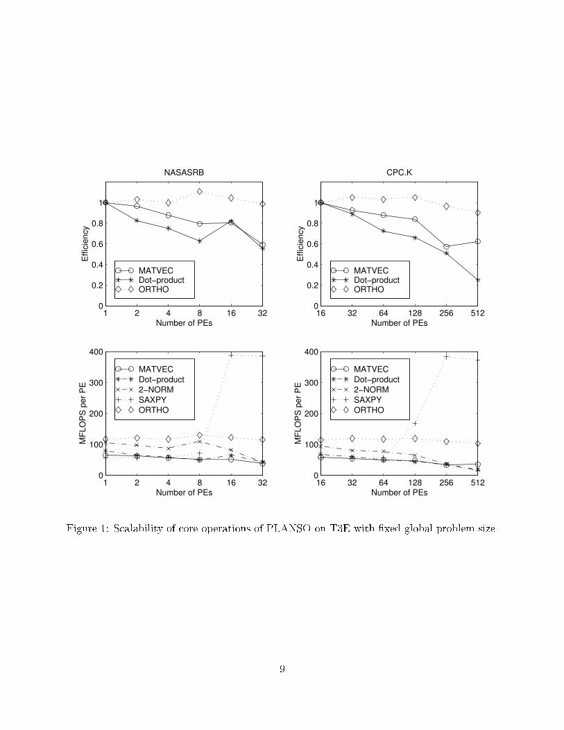
Figure 4: Time to compute the �ve largest eigenvalues of CPC.K with di�erent number ofprocessors.corresponding eigenvectors of CPC.K. In this case, only 40 Lanczos iterations are requiredto �nd the solution during which six re-orthogonalizations are performed. From Figure 1 weknow that the dot-product operation in this case is considerably less e�cient than in theNASASRB test case. In Figure 4 we can see that the time spent in dot-product, SAXPY,etc., can be considerably more than the time spent in matrix-vector multiplication as thenumber of processors increases. In the 512-PE case, out of the 0.34 seconds total time, only0.075 seconds are spent in matrix-vector multiplication, more than 70% of the total timeis used to perform dot-products. Obviously, the e�ciency of the overall parallel Lanczosroutine is low in this case, see Figure 5, because the dominate operation has low parallele�ciency. The e�ciency of PLANSO on 512-PE is 37%, which is above the e�ciency ofthe dot-product (25%), but below the e�ciency of the matrix-vector multiplication routine(62%).As in the NASASRB case, we also tested PARPACK on the CPC.K test problem. Thetiming results are shown in Figure 5. Similar to the NASASRB case, the time taken byPLANSO to �nd the �ve largest eigenvalues is less than that of PARPACK. Part of this isbecause more matrix-vector multiplications are used by the various version of PARPACK,PARPACK(10): 49, PARPACK(20): 43, PARPACK(40): 40. The number of matrix-vector multiplications used by PLANSO is 41. The time di�erence between PLANSO andPARPACK(40) is attributable to the di�erence in the orthogonalization process. When moreprocessors are used, the matrix-vector multiplication time becomes a small portion of thetotal time for both PLANSO and PARPACK. In the PARPACK program, almost all the rest14

16 32 64 128 256 5120.3

1

3

10

Number of PEs

Ela

pse

Tim

e (

se

c)

16 32 64 128 256 51250

100

150

200

250

Number of PEs

All−

PE

Tim

e (

se

c)

16 32 64 128 256 5120

0.2

0.4

0.6

0.8

1

Number of PEs

Eff

icie

ncy

PLANSO PARPACK(10)PARPACK(20)PARPACK(40)

16 32 64 128 256 5120

5

10

15

20

Number of PEs

Sp

ee

d−

up

Figure 5: Comparison between PLANSO and PARPACK on CPC.K test problem.

15

8 27 64 125 216 343 5120

20

40

60

80

100

Number of PEs

MF

LO

PS

pe

r P

E

8 27 64 125 216 343 5120

0.2

0.4

0.6

0.8

1

Number of PEs

Eff

icie

ncy

MATVEC−cube MATVEC−linearDot−product ORTHO

Figure 6: Per PE performances on T3E with �xed local problem size.of the time is spent in Gram-Schmidt orthogonalization which has good parallel e�ciency,see Figure 1. This explains the signi�cant rebound in parallel e�ciency of PARPACK as thenumber of processors becomes large.Overall, PLANSO can maintain above 80% e�ciency on the CPC.K test problem when itis mapped to 64 PEs or less. Similarly, 80% e�ciency can be maintained for the NASASRBtest problem if it is distributed to 16 or less PEs. Mapping CPC.K onto 64 PEs, the problemsize on each PE is about 10,000. Mapping NASASRB onto 16 PEs, the problem size on eachPE is about 3,400. These two examples give us two reference points on what we can expectthe parallel e�ciency to be when mapping a �xed size problem onto di�erent size partitionsof T3E. A moderate local problem size must be maintained in order to maintain reasonablecommunication to computation ratio, therefore to maintain good parallel e�ciency.3.2 Scaled test caseThe intuition on parallel e�ciency is that ideal e�ciency may be achieved if the communi-cation versus computation ratio is maintained constant, or if the problem size on each PEis maintained constant. This is what is shown in Figures 6 and 7. In this case, the parallelLANSO routine is used to �nd the �ve largest eigenvalues and corresponding eigenvectors of�nite di�erence discretization of the Laplacian operator on a 3-D domain. The local problemsize is maintained to be 32,768. As more processors are used the global problem size increasesproportionally. Two di�erent schemes are used to map the global problem onto each PE,one simply divides the matrix as row blocks (linear), the other divides the 3-D domain into sub-cubes and maps the problem on each sub-cube onto a processor. It is clear that the16

8 27 64 125 216 343 51260

65

70

75

80

85

90

Tota

l tim

e (

sec)

linear sub−cube

8 27 64 125 216 343 5120.9

0.95

1

1.05

1.1

Number of PEs

Effic

iency

Figure 7: Scaled performance of PLANSO on 3-D Laplacian test problem.linear mapping requires more data to be exchanged among the processors but each processorneeds to communicate with fewer neighboring processors. Because the linear mapping leadsto large messages being exchanged during matrix-vector multiplication, the matrix-vectormultiplication takes more time than in the sub-cube mapping case. The di�erences in thelocal matrix structure also contribute to the performance di�erence as well. A small partof the performance di�erence also comes from the fact that di�erent packages are used toperform the matrix-vector multiplications. The linear mapping case is done with AZTECand the sub-cube mapping case is done with BLOCKSOLVE95. The intention of doing thisis to show that the parallel LANSO can easily work with di�erent software packages.The performance of the major components of the parallel Lanczos routine is shownin Figure 6. Similar to Figure 1, the performance of the following operations are shown:matrix-vector multiplication, dot-product, SAXPY, and orthogonalization. The e�cienciesof matrix-vector multiplication, dot-product computation and orthogonalization are shownas well. In the bottom plot of Figure 6, the legends are the same as in the plot above. Thethree lines that do not appear in the top plot are:� dash-dot line with cross symbols denotes the performance of computing 2-norm,� dash-dot line with asterisk symbol denotes the performance of computing dot-product,� the dotted line with plus symbols denotes the performance of SAXPY.Most of the lines in Figure 6 are almost straight horizontal lines which indicates that the perPE performance is constant as the number of processors change. The only exception is the17

in-core out-of-core# of PE CGS (sec) MGS (sec) total (sec) I/O time (sec) rate (MB/s)2 4.39 4.75 10.94 5.63 18.14 2.30 2.50 6.82 3.29 29.38 1.27 1.40 5.39 2.70 35.516 0.69 0.77 6.56 3.38 28.532 0.43 0.46 7.60 3.80 25.3Table 1: Performance of an out-of-core versions of parallel LANSO.performance of dot-product and 2-norm computing routines. If the number of processors isnot a power of 2, than their e�ciency can reduce to below 80%.Since the largest eigenvalues of the Laplacian matrix change as matrix sizes change, wehave chosen to run PLANSO for a �xed number of iterations. The time shown in Figure 7 iscollected from running for 602 steps of Lanczos iterations. This number of steps is determinedby allowing the program to take up all the memory of each processing element on the T3E.The 602 Lanczos vectors take up about 160MB of memory which is the amount of memoryleft after the problem is setup on a PE with 256MB of physical memory. Going from 8PE to 512 PE, the matrix-vector multiplication slows down about 15% for both mappingschemes. The total time spent by LANSO is almost exactly the same. This is because thereis a reduction in time spent in re-orthogonalization as the problem size increases and thenumber of converged eigenvalues decreases. The amount of re-orthogonalization requiredin a Lanczos algorithm with partial re-orthogonalization is strongly related to the numberof eigenvalues converged [9, 17]. As more eigenvalues converge, more re-orthogonalizationis needed. As problem size increases, the eigenvalues of Laplacian operator require moreLanczos steps to compute. Thus, within the �rst 602 iterations, less eigenvalue will converge.In the 8-PE case, problem size 262,144, 46 eigenvalues converged within 602 iterations. Inthe 512-PE case, problem size 16,777,216, no eigenvalue converged within 602 iterations.Overall, in this test case, with 64-fold change in the number of processors, the parallele�ciency of PLANSO is better than 90%.3.3 Out-of-core caseTable 1 shows the time used by two versions of parallel LANSO to �nd the �ve largesteigenvalues of NASASRB, one stores the Lanczos vectors in-core, the other out-of-core. Thein-core version also has two di�erent orthogonalization schemes, one uses the classic Gram-Schmidt (CGS) procedure, the other uses the modi�ed Gram-Schmidt (MGS) procedure.The time shown is the average wall-clock time measured on di�erent processors. This testmatrix is small enough that the 75 Lanczos vectors can be store in the main memory of twoT3E processors. In the out-of-core version, each PE stores its own portion of the Lanczosvectors in an unformatted direct access �le using Cray's asynchronous memory cached I/O,cachea, library to interact with the disk system. A large bu�er is used to enhance the I/Operformance. Because the Lanczos vectors are slow to retrieve, we have chosen to use the18

1 4 8 12 160

0.5

1

1.5

2

2.5

Number of PEs

Eff

icie

ncy

MATVEC DOT−productORTHO

1 4 8 12 160

10

20

30

40

50

60

Number of PEs

MF

LO

PS

pe

r P

E

Figure 8: Per PE performance of major components of PLANSO.modi�ed Gram-Schmidt procedure to perform re-orthogonalization. This also increases thenumber of communications required during a re-orthogonalization. The in-core version ofPLANSO uses less time than the out-of-core version. The in-core version with CGS usesslightly less than the one with MGS orthogonalization procedure. The di�erence betweenthem could be larger if more re-orthogonalization were performed. From Table 1, we see thatthe I/O time dominates the total time used by the out-of-core LANSO. The I/O rate is tototal number of byte read/write versus the time used. As the number of processors increases,more I/O processors can be utilized to perform independent read/write operations. Thereare a number of factors that limit the I/O performance. For example, there are only a smallnumber of I/O processors, a disk can only support a �xed number of strides. Typically, thenumber of simultaneous read/write operations is small compared to the number of computingprocessors. This is true for many massively parallel machines.On a massively parallel machine like T3E, out-of-core storage for Lanczos vectors is oftennot necessary. The simple-minded scheme tested here is mainly to show that it is easyto construct an out-of-core version of PLANSO. Since the performance of the out-of-coreLanczos routine is poor, we should consider limiting the maximum memory usage so that allLanczos vectors can �t in-core.19

1 2 4 8 163

10

30

100

Number of PEs

Ela

pse T

ime (

sec)

1 4 8 12 16

50

100

150

200

Number of PEs

All−

PE

Tim

e (

sec)

1 4 8 12 160.5

0.6

0.7

0.8

0.9

1

Number of PEs

Effic

iency

PLANSO PARPACK(25)PARPACK(50)PARPACK(75)

1 4 8 12 16

2

4

6

8

10

12

14

16

Number of PEs

Speed−

up

Figure 9: Performance of PLANSO and PARPACK on a cluster of 2 8-PE SPARC Ultraworkstations.20

4 Performance on cluster of SMPClusters of symmetric multiprocessors (SMP) are used for many di�erent scienti�c and en-gineering applications because they are more economical than massively parallel machines(MPP). We are interested in knowing the performance characteristics of PLANSO on thesetypes of machines. The tests reported in this section are performed on a cluster of 2 8-PESPARC Ultra workstations. The SMP workstations are connected by multiple 622 Mbit/sATM networks using Sun ATM adaptor cards to support parallel programming. At the timeof this test, November 1997, the CPUs of the workstations are 167 Megahertz UltraSPARC Iprocessors with 16 KByte on-board cache and 512 KByte external cache. They were runninga beta version of the Sun HPC clustering software. The tests run here use each individualCPU as an independent processor. No e�ort is made to take advantage of the fact thatsome of them are actually connected on the same bus. We rely on the clustering softwareto handle the non-uniformity in data access. Data communication among the processors isdone using Sun's MPI library. The same Fortran programs used in the T3E test are usedin this test. The BLAS routine from Sun's high performance S3L library is used. All userprograms are compiled with -fast option for the best performance. For more informationabout the cluster, visit http://www.nersc.gov/research/COMPS.The test matrix is NASASRB. As in the MPP case, we show the per PE performance ofthe major components of PLANSO, see Figure 8, and the overall performance of PLANSOon the test problem, see Figure 9. The data shown in Figure 8 is not collected from inside theLanczos routine, but from special testing routines. For dot-product and SAXPY operations,only two vectors are involved. In this test, these vectors can �t into the secondary cachesof 2 or more PEs. This causes a noticeable performance di�erence going from the 1-PEcase to the 2-PE case. Otherwise, most performance curves in Figure 8 are fairly at asthe number of processors change. The exceptions are the lines for computing dot-productand 2-norm. When the number of PE is smaller than nine, all PEs involved are on onebus, the data exchange among them is signi�cantly faster than communicating between theworkstations. The performance of dot-product operation decreases slightly when the numberof PEs involved changes from nine to sixteen. However, the change between the 8-PE caseand the 9-PE case is much larger.Figure 9 shows a number of di�erent measures of the e�ectiveness of the parallel Lanczosroutine, and PARPACK with three di�erent basis sizes. Similar to �gure 3, we show thewall-clock time, the sum of time used by all PEs, the e�ciency and the speed-up of theparallel programs. Comparing the overall e�ciency of PLANSO with the matrix-vectormultiplication routine used, when the number of PEs is less than nine, the e�ciency of theLanczos routine is better than that of the matrix-vector multiplications routine. As morePEs are used, the dot-product operation eventually drags the overall performance down tobelow 80%. On 16 PEs, the speed-up of the Lanczos routine is about 12 (75% e�ciency) andthe speed-up of the matrix-vector multiplication routine is about 13 (81% e�ciency). Thisagain shows that PLANSO can achieve good parallel e�ciency when dot-product routinehas reasonable e�ciency.Comparing the performance of PLANSO with PARPACK, we see that both can achievevery similar parallel e�ciency and speed-up on the test problem. However, because the21

1 4 8 12 160

100

200

300

400

500

600

700

Number of PEs

Ela

pse

Tim

e (

se

c)

PLANSO PARPACK(25)PARPACK(50)PARPACK(75)

Figure 10: Time used by PLANSO on a cluster of 2 8-PE SPARC Ultra workstations.Lanczos routine uses signi�cantly less work in orthogonalization, it uses much less time tosolve the same problem.Figure 10 records the time measured in our tests. The two previous �gures, Figures 8and 9, use only the minimum time measured. The variance in wall-clock time is fairly small,< 5%, when all the processors are on one bus. However, when processors from both SMPare used, the variance can be fairly large. The longest time measured is about an order ofmagnitude larger than the shortest time measured in some cases. This reveals that it is noteasy to achieve consistent high performance on the cluster of SMPs. Some of the reasonsinclude: a parallel job is scheduled as a number of independent tasks on the processorsinvolved, interference from other users both on communication medium and CPU resource,and so on. These types of problems are common to most clusters of SMPs and clusters ofworkstations. There is a signi�cant amount of research on improving job scheduling and otherissues. Clusters of SMPs could eventually be able to consistently deliver the performance ofthe MPP systems.5 SummaryThis report presents our parallel version of LANSO (PLANSO) and measures its perfor-mance on two di�erent platforms. As we have shown in numerical tests, as long as thelocal problem size is not very small, say more than a few thousand, the parallel LANSO canmaintain the parallel e�ciency above that of the matrix-vector multiplication routine. Be-22

cause the Lanczos algorithm uses signi�cantly less arithmetic operations than other similaralgorithms, such as the Arnoldi algorithm, PLANSO solves symmetric eigenvalue problemsin less time than PARPACK. The main reasons are: PLANSO implements the Lanczos algo-rithm with partial re-orthogonalization which reduces the work spent on orthogonalizationto the minimum, and it uses less matrix-vector multiplications because it does not restart.The two platforms on which we performed our tests, the MPP system and Cray T3E,can deliver more consistent performance results. The best speed-up result from solving theNASASRB problem on the cluster of Sun's is very close to the result from the Cray T3Etests, 11.2 versus 11.5. However, the di�erence between the worst measured time and thebest measured time is very large on the cluster of SMPs.The dot-product operation is the one with the lowest parallel e�ciency in the tests pre-sented. This indicates to us that enhancing its e�ciency could signi�cantly enhance overalle�ciency. One commonly used scheme is a block version of the Lanczos algorithm. Otheralternatives include rearranging the algorithm so that the two dot-product computationscan be done with only one global reduction operation, and so on. These alternatives will beconsidered in the future.On some parallel environments, such as Cray T3E, the I/O performance does not growproportional to the number of processors used for computing. In this case, considerable e�ortmay be required to develop a scalable out-of-core Lanczos method. The simple out-of-corePLANSO tested does not scale well on T3E. If a large number of Lanczos steps are neededto compute a solution, PARPACK could be more e�ective because the user can limit themaximum memory usage by restarting the Arnoldi algorithm. The restarting scheme letsPARPACK use more matrix-vector multiplications but smaller amounts of memory to �ndthe solution. This is a common trade-o� that could bene�t the Lanczos algorithm as well.From the tests, we also identi�ed that the dot-production operation can be a bottleneckfor scalability of the parallel Lanczos algorithm. Reducing the cost of dot-product operationcould signi�cantly enhance the overall performance of the Lanczos algorithm.PLANSO can also be easily used with di�erent parallel sparse matrix packages. In thisreport we have shown examples of using PLANSO with P SPARSLIB, AZTEC and BLOCK-SOLVE. The example programs used in this report are also available with the distribution ofthe source code of PLANSO at http://www.nersc.gov/research/SIMON/planso.tar.gz.6 AcknowledgmentsThe MPP tests were performed on the Cray T3E at National Energy Research Scienti�cComputing Center (NERSC). The cluster of SMPs used was established by a joint researchproject between NERSC, UC Berkeley, Sun Microsystems, and the Berkeley Lab Informationand Computing Sciences Division (ICSD) and Materials Sciences Division (MSD).Appendix Interfaces of parallel LANSOThe interface to the main access points of the parallel LANSO package are similar to theirsequential counterparts. The two main entries are named PLANDR and PLANSO, they are the23

parallel counterparts of LANDR and LANSO of the LANSO package. The di�erence is that anew argument named MPICOM is attached to the end of the calling sequences, see below.SUBROUTINE PLANDR(N,LANMAX,MAXPRS,CONDM,ENDL,ENDR,EV,KAPPA,& J,NEIG,RITZ,BND,W,NW,IERR,MSGLVL,MPICOM)INTEGER N,LANMAX,MAXPRS,EV,J,NEIG,NW,IERR,MSGLVL,MPICOMREAL*8 CONDM,ENDL,ENDR,KAPPA,& RITZ(LANMAX),BND(LANMAX),W(NW)SUBROUTINE LANSO(N,LANMAX,MAXPRS,ENDL,ENDR,J,NEIG,RITZ,BND,& R,WRK,ALF,BET,ETA,OLDETA,NQ,IERR,MSGLVL,MPICOM)INTEGER N,LANMAX,MAXPRS,J,NEIG,NQ(4),IERR,MSGLVL,MPICOMREAL*8 ENDL,ENDR,R(5*N),WRK(*), ETA(LANMAX),OLDETA(LANMAX)& ALF(LANMAX),BET(LANMAX+1),RITZ(LANMAX),BND(LANMAX)The arguments are as follows,� N (INPUT) The local problem size.� LANMAX (INPUT) Maximum Lanczos steps. If the LANSO routine does not �nd MAXPRSnumber of eigenvalues, it will stop after LANMAX steps of Lanczos iterations.� MAXPRS (INPUT) Number of eigenvalues wanted.� CONDM (INPUT) Estimated e�ective condition number of operator M .� ENDL (INPUT) The left end of interval containing unwanted eigenvalues.� ENDR (INPUT) The right end of interval containing unwanted eigenvalues.� EV (INPUT) Eigenvector ag. Set EV to be less or equal to 0 to indicate that noeigenvector is wanted. Set it to a natural number to indicate that both eigenvalues andeigenvectors are wanted. When eigenvectors are wanted, they are written to FortranI/O unit number EV without formatting.� KAPPA (INPUT) Relative accuracy of the Ritz values. It is only used when eigenvectorsare computed, in which case an eigenpair is declared converged if the error estimate isless than �j�j. If eigenvector is not wanted, an eigenvalue is declared converged whenits error is less than 16�j�j, where � the machine's unit round-o� error. In fact, thesubroutine PLANSO always use this as convergence test. KAPPA is only used in subroutineRITVEC which computes Ritz vectors when the user requested the eigenvectors, EV > 0.� J (OUTPUT) Number of Lanczos steps taken.� NEIG (OUTPUT) Number of eigenvalues converged.� RITZ (OUTPUT) Computed Ritz values.� BND (OUTPUT) Error bounds of the computed Ritz values.24

� W (INPUT) Workspace. On input, the �rst N elements is assumed to contain the initialguess r0 for the Lanczos iterations.� NW (INPUT) Number of elements in W. It must be at least 5 � N + 4 � LANMAX +max(N; LANMAX + 1)+1 when no eigenvector is desired. Otherwise an additional LANMAX�LANMAX elements is needed.� IERR (OUTPUT) Error code from TQLB, a modi�ed version of TQL2 from EISPACK[8].� MSGLVL (INPUT) Message level. The larger it is, the more diagnostic message is printedby LANSO. Set it to zero or smaller to disable printing from LANSO, set it to 20 orlarger to enable all printing.� MPICOM (INPUT) MPI communicator used. All members of this MPI group will par-ticipate in the solution of the eigenvalue problem.The following items are in the argument list of PLANSO but not in the argument list of PLANDR.They are part of workspace W. PLANDR checks the size of W and splits it correctly before callingPLANSO. It also provides the extra functionality of computing the eigenvectors after returningfrom PLANSO. We encourage the user to use PLANDR rather than directly calling PLANSO.� R holds 5 vectors of length N.� NQ contains the pointers to the beginning of each vector in R.� ALF holds diagonal of the tridiagonal T , �i.� BET holds o�-diagonal of T , �i.� ETA holds orthogonality estimate of Lanczos vectors at step i.� OLDETA holds orthogonality estimate of Lanczos vectors at step i� 1.� WRK miscellaneous usage, size max(N; LANMAX + 1).As mentioned before, the matrix operations are performed through two �xed-interfacefunctions. They are as follows:SUBROUTINE OP(N,S,Q,P)SUBROUTINE OPM(N,Q,S)INTEGER NREAL*8 P(N), Q(N), S(N)The subroutine OPM computes s = Mq, where Q and S are local components of the inputvector q and output vector s. The subroutine OP computes p = M�1Kq, where s = Mqis passed along in case it is needed. The subroutine OP may alternatively compute p =(K � �M)�1Mq in order to compute eigenvalues near �. To �nd the eigenvalues of asymmetric matrix A, OPM simply copies Q to S, OP computes p = Aq.LANSO stores and retrieves old Lanczos vectors through the STORE function which isassumed to have the following interface. 25

SUBROUTINE STORE(N,ISW,J,S)INTEGER N,ISW,JREAL*8 S(N)The argument N is the local problem size, ISW is a switch that can take on one of the followingfour values: 1, 2, 3, or 4 which means store qj(1), retrieve qj(2), store Mqj(3), and retrieveMqj(4), argument J is the aforementioned index j, and local components of input/outputvector are stored in S. Through this routine, LANSO may store the Lanczos vectors in-core orout-of-core. Normally, storing the Lanczos vectors in-core means that they can be retrievedmuch faster than storing them out-of-core. However, since the Lanczos iteration may extendmany steps before the wanted eigenvalues are computed to satisfactory accuracy, it may notbe possible to store the Lanczos vectors in-core. The user is required to provide an e�ectiveroutine to store the Lanczos vectors.The partial re-orthogonalization scheme implemented in LANSO orthogonalizes the lasttwo Lanczos vectors against all previous Lanczos vectors when a signi�cant loss of orthogonal-ity is detected. It does so by retrieving each of the previous Lanczos vectors and orthogonalizethe two vectors against the one retrieved. If the norm of the vector after orthogonalization issmall, the orthogonalization may be repeated once. The parallel LANSO package providesa default re-orthogonalization that uses the STORE function to access each Lanczos vectorand perform a modi�ed Gram-Schmidt procedure. A faster orthogonalization routine canbe constructed by the user since the user knows where the Lanczos vectors are stored. Forexample, on parallel machines, if the Lanczos vectors are stored in-core, the user may use theclassic Grid-Schmidt procedure rather than modi�ed Grid-Schmidt procedure. This allowsthe global sum operations of all the inner-products to be performed at once, which reducesthe communication overhead in orthogonalization. The user may not have to replace thisroutine if the re-orthogonalization is rear and a relatively small percentage of total timeis spent in it. However, in many cases, re-orthogonalization occurs every 5 to 10 Lanczositerations near the end, the time spent in re-orthogonalization may be signi�cant part of theoverall computation. In these cases, the user should consider replacing the orthogonaliza-tion routine PPURGE to enhance the performance of the eigenvalue routine. Examples of themodi�ed PPURGE functions are provided along with various examples of using the parallelLANSO code.LANSO was designed to compute a few eigenvalues outside of a given range which issuitable to �nd eigenvalues near � using the shift-and-invert operator (K��M)�1M . Oftenone only wants a few smallest or largest eigenvalues and corresponding eigenvectors. Forthis purpose, an alternative interface to LANSO is provided.SUBROUTINE PLANDR2(N,LANMAX,MAXPRS,LOHI,CONDM,KAPPA,& J,NEIG,RITZ,BND,W,NW,IERR,MSGLVL,MPICOM)INTEGER N,LANMAX,MAXPRS,LOHI,J,NEIG,NW,IERR,MSGLVL,MPICOMREAL*8 CONDM,KAPPA,& RITZ(LANMAX),BND(LANMAX),W(NW)When LOHI is greater than 0, it computes MAXPRS largest eigenvalues, otherwise it attemptsto compute MAXPRS smallest eigenvalues. It does not attempt to compute eigenvectors, but26

instead it places �i and �i at the front of W before returns to caller. This allows easy accessto �i and �i which is needed to compute the eigenvectors. This version of LANSO alwaysuses KAPPA in convergence test in the same fashion as in ARPACK, i.e., an eigenvalue �i isconsidered converged if its error bound is less than �j�ij or ��2=3. This alternative interfacecan provide exactly the same functionality as PARPACK's routine for symmetric eigenvalueproblems.References[1] S. Balay, W. Gropp, L. C. McInnes, and B. Smith. PETSc 2.0 users man-ual. Technical Report ANL-95/11, Mathematics and Computer Science Divi-sion, Argonne National Laboratory, 1995. Lastest source code available at URLhttp://www.mcs.anl.gov/petsc.[2] F. Chatelin. Eigenvalues of Matrices. Wiley, 1993.[3] J. Cullum and R. A. Willoughby. Lanczos Algorithms for Large Symmetric EigenvalueComputations: Theory, volume 3 of Progress in Scienti�c Computing. Birkhauser,Boston, 1985.[4] J. Cullum and R. A. Willoughby. Lanczos Algorithms for Large Symmetric EigenvalueComputations: Programs, volume 4 of Progress in Scienti�c Computing. Birkhauser,Boston, 1985.[5] I. S. Du�, A. M. Erisman, and J. K. Reid. Direct Methods for Sparse matrices. OxfordUniversity Press, Oxford, OX2 6DP, 1986.[6] I. S. Du�, R. G. Grimes, and J. G. Lewis. Sparse matrix test problems. ACM Trans.Math. Soft., pages 1{14, 1989.[7] G. H. Golub and C. F. van Loan. Matrix Computations. The John Hopkins UniversityPress, Baltimore, MD 21211, thrid edition, 1996.[8] B. S. Grabow, J. M. Boyle, J. J. Dongarra, and C. B. Moler, editors. Matrix EigensystemRoutines | EISPACK Guide Extension. Number 51 in Lecture Notes in ComputerScience. Springer, New York, 2nd edition, 1977.[9] R. G. Grimes, J. G. Lewis, and H. D. Simon. A shifted block Lanczos algorithmfor solving sparse symmetric generalized eigenproblems. SIAM J. Matrix Anal. Appl.,15(1):228{272, 1994.[10] S. A. Hutchinson, J. N. Shadid, and R. S. Tuminaro. AZTEC user's guide. Tech-nical Report SAND95-1559, Massively parallel computing research laboratory, SandiaNational Laboratories, Albuquerque, NM, 1995.[11] M. T. Jones and P. E. Plassmann. Blocksolve95 users manual: scalable library softwarefor parallel solution of sparse linear systems. Technical Report ANL-95/48, Mathematicsand Computer Science Division, Argonne national alboratory, Argonne, IL, 1995.27

[12] B. N. Parlett and D. Scott. The Lanczos algorithm with selective orthogonalization.Math. Comp., 33:217{2388, 1979.[13] Beresford N. Parlett. The symmetric eigenvalue problem. Prentice-Hall, EnglewoodCli�s, NJ, 1980.[14] Y. Saad and K. Wu. Design of an iterative solution module for a parallel matrix library(P SPARSLIB). Applied Numerical Mathematics, 19:343{357, 1995. Was TR 94-59,Department of Computer Science, University of Minnesota.[15] Yousef Saad. Numerical Methods for Large Eigenvalue Problems. Manchester UniversityPress, 1993.[16] Yousef Saad. Iterative Methods for Sparse Linear Systems. PWS publishing, Boston,MA, 1996.[17] Horst D. Simon. The Lanczos algorithm for solving symmetric linear systems. PhDthesis, University of California, Berkeley, 1982.[18] D. Sorensen, R. Lehoucq, P. Vu, and C. Yang. ARPACK: an implementation ofthe Implicitly Restarted Arnoldi iteration that computes some of the eigenvalues andeigenvectors of a large sparse matrix. Available from ftp.caam.rice.edu, directorypub/people/sorensen/ARPACK, 1995.[19] L.-W. Wang and A. Zunger. Large scale electronic structure calculations using theLanczos method. Computational Materials Science, 2:326{340, 1994.[20] F. Webster and G.-C. Lo. Projective block Lanczos algorithm for dense, Hermitianeigensystems. J. Comput. Phys., pages 146{161, 1996.

28