a numerical study on the effect of length to diameter...

Australian Journal of Basic and Applied Sciences, 4(10): 4943-4957, 2010ISSN 1991-8178

A Numerical Study on the Effect of Length to Diameter Ratio and Stagnation Pointon the Performance of Counter Flow Ranque-hilsch Vortex Tubees

1Abdolreza Bramo, 1,2Nader Pourmahmoud

1Department of Mechanical Engineering, Urmia University, Urmia, Iran.

Abstract: In this numerical study, performance of Ranque-Hilsch vortex tubes, with a length todiameter ratios (L/D) of 8, 9.3, 10.5, 20.2, 30.7, and 35 with six straight nozzles, on the basis ofexperimental results were investigated. Also, this study has been done to understanding the effects ofstagnation point location on the performance of RHVT. CFD analysis is employed to achieve thehighest temperature separation and optimum length to diameter (L/D) ratio of the Ranque–Hilschvortex tubes. The temperature separation phenomenon in the vortex tube has been obtained by a 3Dcompressible turbulent CFD model. It was found that the best performance was obtained when theratio of vortex tube’s length to the diameter was 9.3 and also at this model the stagnation point wasfound the farthest from the inlet. The results showed that the closer distance to the hot end willprovide large amounts of temperature difference. The location of stagnation point calculated by thetwo methods and were compared for various lengths of vortex tubes. Moreover, it is found thatincreasing the cold mass fraction decreases the cold temperature difference and efficiency. Finally thecomputed results such as velocity and temperature variations calculated and discussed in more details.Presented results in this paper shown good agreement with experimental results.

Key words: Ranque-Hilsch vortex tube, Stagnation point, Length effects, CFD .

INTRODUCTION

Ranque–Hilsch vortex tube is a device with a simple geometry and without any intricacy, which canproduce temperature separation. When a vortex tube is injected with compressed air through some tangentialnozzles into its vortex chamber, a strong rotational flow field is established. This vortex in the inlet area causespressure distribution of the flow in radial direction. As a result a free vortex is produced as the peripheralwarm stream and a forced vortex as the inner cold stream. After energy separation in the vortex tube, the inletair stream was separated into two air streams: hot air stream and cold air stream, the hot air stream left thetube from one end and the cold air stream left from another end. Fig. 1(a) shows the schematic diagram ofa vortex tube and its flow pattern. Vortex tubes were discovered in 1932 by Ranque, (1933). later Hilsch,(1946) performed

NomenclaturesCFD Computational fluid dynamicsD Diameter of vortex tube (mm)dc Cold end diameter (mm)k Turbulence kinetic energy (m2 s-2)L Length of vortex tube (mm)m Mass flow rate (g s-1)r Radial distance from axis(mm)T Temperature (K)z Axial length from nozzle cross sectionDTch Temperature difference between cold and hot end(K)DTic Temperature difference between inlet and cold end(K)DThi Temperature difference between hot end and inlet(K)

Corresponding Author: Abdolreza Bramo, Department of Mechanical Engineering, Urmia University, Urmia,Iran.

Email: [email protected]

Aust. J. Basic & Appl. Sci., 4(10): 4943-4957, 2010

Greek Symbolsa Cold gas fraction.e Turbulence dissipation rate (m2 s-3)m Dynamic viscosity (kg m-1 s-1)mt Turbulent viscosity (kg m-1 s-1)r Density (kg m-3) s Stress (N m-2) t Shear stress (N m-2) tij Stress tensor components Subscriptsc Cold gas h Hot gasi Inlet in vortex tubethe detailed examination of the Ranque effect and conducted experiments by varying the inlet pressure and thegeometrical parameters of the tube. Since then, the vortex tube has been a subject of much interest. Harnettand Eckert, (1957) invoked turbulent eddies, Ahlborn and Gordon, (2000) described an embedded secondarycirculation and Stephan et al. (1983) proposed the formation of Gortler vortices on the inside wall of the vortextube that drive the fluid motion. Kurosaka, (1982) reported the temperature separation to be a result of acousticstreaming effect that transfer energy from the cold core to the hot outer annulus. Aljuwayhel et al. (2005)utilized a fluid dynamics model of the vortex tube to understand the process that drives the temperatureseparation phenomena. Skye et al. (2006) used a model similar to that of Aljuwayhel et al. (2005). Chang HSohn et al. (2006) conducted a visualization experiment using surface tracing method to investigation theinternal flow phenomena and to indicate the stagnation position in a vortex tube.Ameri et al. (2010) and Eismaet al. (2007) performed a numerical study to research the flow field and temperature separation phenomenon.Also some studies has been done to use vortex tube as a refrigeration system, instead of the conventionalrefrigeration systems. Alka Bani Agrawal; Vipin Shrivastava, (2010). and Jayaraman, Senthil Kumar, (2010).Volkan kirmaci, (2009) used Taguchi method to optimize the number of nozzle of vortex tube. While each of

Fig. 1: (a)Flow pattern and schematic diagram of vortex tube (b) Schematic of an ExairTM 708 slpm modelvortex tube

these explanations may capture certain aspects of vortex tube, none of these mechanisms altogether explainsthe vortex tube effect. Vortex tubes generally are used as a cooling system for Industrial purposes.

2. Numerical Modeling:The numerical simulation of the vortex tube has been created by using the FLUENTTM software package.

The models are three dimensional, steady state, compressible and employ the standard k-epsilon turbulencemodel. The RNG k-epsilon turbulence model and more advanced turbulence models such as the Reynolds stressequations were also investigated, but these models could not be made to converge for this simulation yet. Thecompressible turbulent flows in the vortex tube are governed by the conservation of mass, momentum andenergy equations. The mass and momentum conservation and the state equation are solved as follows:

4944


(1)j( ) ( ) 0

jt ux� ��

� � �

(2)( ) ( )i j i ij

j i

pt u u ux x� � ��

� � � ��

2.1. Turbulence Model:The flow field inside the vortex tube is fully turbulent. Thus the turbulence kinetic energy, k and its rate

of dissipation, � are obtained from the following transport equations:

(3)( ) ( )ii

k kt ux� ��

� ��

[( ) ]tMk b

j k j

k G G Yx x� ��

� ��

� �and

( ) ( ) [( ) ]ti

i j j

k kt ux x x

� � ��

� � � ��

� � � �

(4)2

1 3 2( )k bk kC G C G C

� � � �

Where, Gk represents the generation of turbulence kinetic energy due to the mean velocity gradients, Gb is thegeneration of turbulence kinetic energy due to buoyancy, YM represents the contribution of the fluctuatingdilatation in compressible turbulence to the overall dissipation rate, C1�, C2� and C3� are coefficients. �k and�� are the turbulent prandtl numbers for k and �, respectively. The turbulent viscosity, �t is computed bycombining k and � as follows:

(5)2

tkC �

��

Where, C� is a constant. The model constants C1�, C2�, C�, �k and �� have the following default values: C1�= 1.44, C2� = 1.92, C� = 0.09, �k = 1.0, �� = 1.3

Fig. 2: (a)Three-dimensional model of vortex tube with six straight nozzles provided with refinement in mesh(b) A part of sector that taken for analysis showing computational domain

3. Physical Modeling:The present CFD model was created based on the model which used by Skye et al., (2006). It is

noteworthy that, an ExairTM 708 slpm vortex tube was used by Skye et al., (2006) to collect all of theexperimental data which is shown in Fig.1 (b). The geometry summary of the vortex tube which used by Skyeet al., (2006) is given in Table 1.

In addition to the model which was used by Skye et al., (2006), to study the effects of length on theperformance of vortex tube, all geometrical properties of the Skye et al., (2006) model are kept constant, andonly with changing the length of the model, five other models with different lengths were created . So,following analysis is made for specific vortex tube with six numbers of straight nozzles and various L/D ratios.In this numerical simulation the radius of the vortex tubes fixed at 5.7 mm for all the models, and the lengthare set to 92, 106, 120, 230, 350, and 400 mm respectively. Since the nozzle consists of 6 straight slots, the

4945


Table 1: Geometry summary of the vortex tube which was used in experiment (ExairTM 708 slpm)Measurement ValueWorking tube length 106 mmNozzle height 0.97 mmNozzle width 1.41 mmNozzle total inlet area (An) 8.2 mm2

Cold exit diameter 6.2 mmCold exit area 30.3 mm2

Hot exit diameter 11 mmHot exit area 95 mm2

CFD model assumed to be a rotational periodic flow and only a sector of the flow domain with angle of 60°,needs to be considered which is shown in Fig2(b). The three-dimension model showing boundary regions isshown in Fig. 2(a) and (b). Thus, performance of vortex tubes, with a length to diameter ratio of 8, 9.3, 10.5,20.2, 30.7, and 35were investigated. The analysis has been done to achieve the optimum length to diameterratio (L/D), between six various lengths of vortex tubes.

3.1. Boundary Conditions for Analysis:Boundary conditions for the model were determined based on the experimental measurements by Skye et

al., (2006) for all case in this analysis. The inlet is modeled as a mass flow inlet; the total mass flow rate,stagnation temperature, were specified and fixed at 8.35 g sec�1, 294.2 K respectively. The static pressure atthe cold exit boundary was fixed at experimental measurements pressure. The static pressure at the hot exitboundary was adjusted to vary the cold fraction. A no-slip boundary condition is enforced on all walls of thevortex tube. Fig. 4 shows the reversed flow at cold exit, since the CFD model predicts that reversed flow willoccur at the cold exit at low cold gas fractions, then the backflow temperature value is set to 290 k.

RESULTS AND DISCUSSION

CFD analyses were carried out for a 11.4 mm diameter vortex tube with L/D of 8, 9.3, 10.5, 20.2, 30.7,and 35 shows the existence of an optimum length according to the boundary and operating conditions, thatmust be determined, to achieve the maximum efficiency of vortex tube. The results showed that, the bestperformance is obtained when the length to diameter ratio is 9.3(L=106 mm). Notice that this is the samemodel that was used by skye et al. (2006). The obtained results for optimum case (106mm) were comparedand validated with experimental and numerical results of skye et al. (2006) (Fig.3 and 4).

Also, the effects of stagnation point position, on the performance of vortex tubes were investigated .It wasconcluded that, the stagnation point position affects on the performance of vortex tubes significantly. Theresults verify that, the closer distance to the hot end will provide large amounts of temperature difference. Alsothe study results showed that stagnation point is the nearest to the hot end at optimum case of present study(L=106 mm), compared to the other models.

Discussion:

Fig. 4: Reversed flow through cold exit at low cold gas fraction

4946


Fig. 3: Comparison of cold temperature difference obtained at present CFD simulation and Skye et al., (2006)simulation and experiments

Fig. 4: Comparison of hot temperature difference obtained at present CFD simulation and Skye et al., (2006)simulation and experiments

Effect of Length to Diameter Ratio:As shown in Fig.3 and 4, the obtained temperature difference at present analysis for the optimum vortex

tube (L=106 mm), were compared with the experimental and computational results of Skye et al. (2006), thatboth models have similar geometry, inlet and boundary conditions. It must be said that the Skye et al. (2006) CFD model was developed using a two-dimensional, and the present CFD models are three dimensional. Asshown in Fig. 4 the hot exit temperature difference, �Th,i ,predicted by the our model is in good agreementwith the experimental results. Prediction of the cold exit temperature difference �Ti,c for optimum model ofpresent study is found to lie between the experimental and computational result of Skye et al. (2006) that isshown in Fig. 3. Compared to the present calculations k-� model predictions with computational results of skyeet al. (2006), clearly observed that the hot exit temperature difference �Th,i simulated at both models wereclose to the experimental results. Though both models get values less than experimentally results of cold exittemperature difference �Ti,c, but the predictions from the present model were found closer to experimentalresults. As seen in Fig. 3, the maximum temperature drop at cold exit of vortex tube is obtained at cold gasfraction of about 0.3 through the experiment and CFD simulation.

The magnitude of swirl velocity is one of most important factors that affect performance of vortex tube.The optimum length of present calculation (L=106mm) can produce maximum swirl generation of 428 m/s atinlet zone, and hot gas temperature of 363.2 K at 0.8 of cold gas fraction, and a minimum cold gastemperature of 250.24 K at about 0.3 cold gas fraction. The results of analysis for all vortex tube lengths thatwere investigated, are given in Table 2.

4947


Table 2: The results of CFD analysis for all vortex tubes lengths that investigated at a=0.3(maximum cooling effect)(L/D) L (mm) Vsm(m/s) Tcm (K) Thm (K) �T i,c (K) �T h,i (K) �Tch (K)8 92 390 254.77 310.56 39.48 16.36 55.849.3 106 428 250.24 311.5 43.96 17.3 61.2610.5 120 390 254.72 309.45 39.48 15.25 54.7320.2 230 387 254.9 310.7 39.3 16.5 55.830.7 350 388 255.05 310.33 39.15 16.13 55.2835 400 388 254.94 310.68 39.26 16.48 55.74 L/D: length to diameter ratio L: Length of tube Thm: Maximum temperature at hot endTcm: Minimum temperature at cold end Vsm: Maximum generated swirl velocity �Th,i: Temperature separation between inlet and hot end�Ti,c: Temperature separation between inlet and cold end�Tch: Temperature separation between cold and hot end

Fig. 5: Radial profiles of axial velocity at different axial locations for a=0.3 : (a)z/l=0.1 (b)z/l=0.4 (c)z/l=0.7

4948


Fig. 6: Radial profile of swirl velocity at different axial locations for a=0.3 : (a)z/l=0.1 (b)z/l=0.4 (c)z/l=0.7

Fig. 5 shows the radial profiles of the axial velocity at different axial locations (z/l = 0.1, 0.4 and 0.7)at specified cold gas fraction of 0.3 (a=0.3), for various length of vortex tubes. It was observed that themaximum value of the axial velocity decreased with increasing axial distance from the inlet zone. For optimumvortex tube (L=106mm) at axial locations of z/l=0.1, 0.4 and 0.7 the maximum axial velocity was found 83,63 and 57 m s�1 respectively, therefore a maximum value of 83 m/s is seen at the tube axis near the inlet zone(z/l=0.1).

Fig. 6 shows the radial profiles for the swirl velocity (tangential velocity) at different axial locations(z/l=0.1, 0.4 and 0.7). Comparing the velocity components, it is observed that swirl velocity has the highestvalue and decreases in amplitude towards the hot end exit. The radial profile of the swirl velocity indicatesa free vortex near the wall and the values become negligibly small at the core, which is in conformity withthe observations of Kurosaka, (1982), Gutsol, (1997). Also the axial and swirl velocity profiles obtained atdifferent axial locations of the vortex tube are in good conformity with observations of Gutsol, (1997) andBehera, (2005). According to variations of the swirl velocity which is shown in Fig. 6, in near of the inletzone (z/l=0.1), compared to other models the highest swirl velocity belongs to model with L=106mm, but withincreasing the distance from inlet zone towards the hot end, the swirl velocity magnitude decrease in allmodels.

4949


Fig. 7: Flow pattern sections for optimum RHVT: (a) near cold exit end (b) in mid region along the axialdirection (c) near hot exit end

The flow patterns for optimum vortex tube of present investigation (L=106mm) at sectional lengths nearthe cold and hot exits and in mid region of vortex tube are shown in Fig. 7. The core and peripheral flow canbe clearly seen at near cold end and mid region but at near hot end shows only the presence of peripheral flowtowards the hot end

Fig. 8: Streamlines inside of vortex tube colored by total temperature.

Fig. 9: Contours of total temperature at: cold exit, z/l=0.1,z/l=0.4,z/l=0.7, hot exit.

The total temperature distribution from CFD analysis along the length of tube, for the optimum vortex tubewith length to diameter ratio of 9.3 (L=106mm) is displayed in Fig. 9and 11. Clearly can be seen thatperipheral flow is warm and core flow is cold, furthermore increasing of temperature is seen in radial direction.

4950


The optimum length of this study, for a cold gas fraction of about 0.3, gives the maximum hot gas temperatureof 311.5 K and minimum cold gas temperature of 250.24 K .Also, the three dimensional path lines of flowinside the vortex tube and rotational flow pattern is presented in Fig. 9.

Fig. 10: Radial profiles of total temperature at different axial locations for a=0.3(maximum cooling effect):(a) z/l=0.1 (b) z/l=0.4 (c) z/l=0.7.

Radial profiles of the total temperature at various axial location (z/l = 0.1, 0.4 and 0.7) for different lengthof vortex tube are presented in Fig.10. The maximum total temperature was observed to exist near theperiphery of the tube wall in all vortex tubes. At the tube wall the total temperature is found to decrease, thisis due to the no slip boundary condition at the tube wall. The predicted temperature profiles are a result ofthe kinetic energy distribution in the vortex tube. The fluid at the core of the vortex tube has very low kineticenergy due to the minimum swirl fluid velocity at the central zone of the tube. From the swirl velocity profilesFig. 6 it was observed that the swirl velocity had almost negligible value at the core of the vortex tube.Comparing the total temperature and the swirl velocity profiles (Fig. 6and 10) show that the low temperaturezone in the core coincides with the negligible swirl velocity zone. The total temperature profiles (Fig.10) showsan increase of the temperature values towards the periphery. As seen in Fig.10 (a) and(c), the model withL=106mm shows minimum cold gas temperature at cold exit and maximum hot gas temperature at hot exit.

Fig. 11: Temperature distribution in axial direction of optimum vortex tube in sections

Fig. 12 shows the CFD analysis data on temperature difference between hot and cold end (?Tch) fordifferent L/D ratios. It can be noted that the peak value in ?Tch is obtained for L/D ratio of 9.3(L=106mm)that investigated by skye et al. (2006) experimentally and present numerical study. Fig. 13 shows thetemperature difference at cold exit end for various lengths of vortex tube,which were investigated . Comparingthe various lengths of vortex tube it is observed that the model with length of 106 mm has the maximumtemperature separation about 43.96 K, at cold exit.

4951


Fig. 12: Temperature difference between hot and cold gas for different L/D ratios

Fig. 13: Temperature difference at cold exit for different lengths of vortex tubes

5.2. Stagnation Point Effect;The results of present study shows that the performance of vortex tubes related to stagnation point location

and the location of the stagnation point is related to the geometric design of the vortex tube, and also studyabout length effect required to exploration of the stagnation point location along the tube to achieve theoptimum length and highest energy separation. The results shows that increase in the length of tube, improvethe temperature separation up to the condition that stagnation point is within the length of tube

Fig. 14: Schematic flow pattern of Ranque–Hilsch tube

CFD analysis were carried out for a 11.4 mm diameter vortex tube with L/D of 9.3, 10.5, 20.2, 30.7, and35 with six straight nozzles, based on the experimental measurements of Skye et al, (2006) to determine thestagnation point position along the tube and to study the influence of stagnation point position on thetemperature separation in the vortex tube. The stagnation point position within the vortex tube can bedetermined by two ways: according to maximum wall temperature and on the basis of velocity profile along

4952


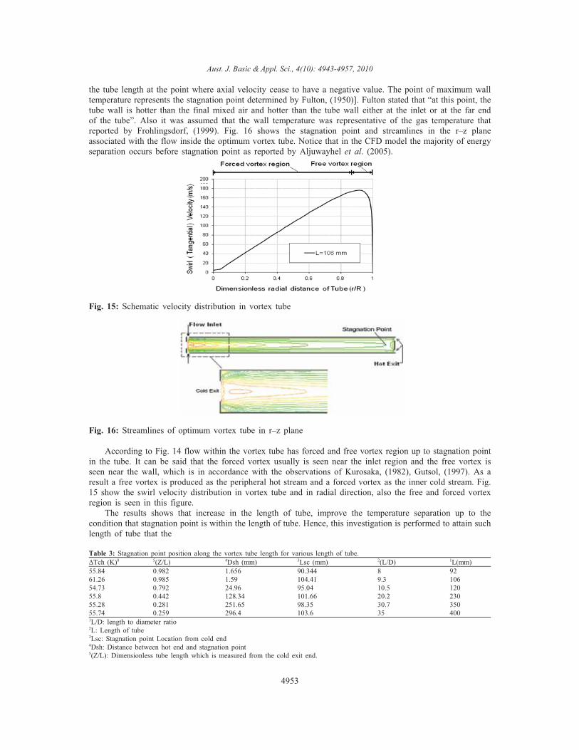
the tube length at the point where axial velocity cease to have a negative value. The point of maximum walltemperature represents the stagnation point determined by Fulton, (1950)]. Fulton stated that “at this point, thetube wall is hotter than the final mixed air and hotter than the tube wall either at the inlet or at the far endof the tube”. Also it was assumed that the wall temperature was representative of the gas temperature thatreported by Frohlingsdorf, (1999). Fig. 16 shows the stagnation point and streamlines in the r–z planeassociated with the flow inside the optimum vortex tube. Notice that in the CFD model the majority of energyseparation occurs before stagnation point as reported by Aljuwayhel et al. (2005).

Fig. 15: Schematic velocity distribution in vortex tube

Fig. 16: Streamlines of optimum vortex tube in r–z plane

According to Fig. 14 flow within the vortex tube has forced and free vortex region up to stagnation pointin the tube. It can be said that the forced vortex usually is seen near the inlet region and the free vortex isseen near the wall, which is in accordance with the observations of Kurosaka, (1982), Gutsol, (1997). As aresult a free vortex is produced as the peripheral hot stream and a forced vortex as the inner cold stream. Fig.15 show the swirl velocity distribution in vortex tube and in radial direction, also the free and forced vortexregion is seen in this figure.

The results shows that increase in the length of tube, improve the temperature separation up to thecondition that stagnation point is within the length of tube. Hence, this investigation is performed to attain suchlength of tube that the

Table 3: Stagnation point position along the vortex tube length for various length of tube.�Tch (K)8 5(Z/L) 4Dsh (mm) 3Lsc (mm) 2(L/D) 1L(mm)55.84 0.982 1.656 90.344 8 92 61.26 0.985 1.59 104.41 9.3 106 54.73 0.792 24.96 95.04 10.5 120 55.8 0.442 128.34 101.66 20.2 230 55.28 0.281 251.65 98.35 30.7 35055.74 0.259 296.4 103.6 35 4001L/D: length to diameter ratio 2L: Length of tube 3Lsc: Stagnation point Location from cold end 4Dsh: Distance between hot end and stagnation point 5(Z/L): Dimensionless tube length which is measured from the cold exit end.

4953


stagnation point is inside of tube. In this our study the vortex tube with L = 106 mm (L/D =9.3) presentedthe highest temperature separation between all the other models. Also the results of present investigation thatgiven in table. 3 shows the distance between stagnation point and hot end at vortex tube with length of 106mm (L/D =9.3) is lowest compared to all other models. Since the vortex tube with length of 106mm presentedthe highest temperature separation compared to other models, then as a result of this study can be said thedistance of between hot end and stagnation point is an important factor that affect the performance of vortextubes. Thus, less distance between hot end and stagnation point causes more temperature separation.

Fig. 17: Variation of axial velocity along the center line of the vortex tube :( a) L=92mm (b) L=106mm (c)L=120mm (d) L=230mm (e) L=350mm (f) L=400mm

The variations of axial velocity along the center line of the vortex tube for six different lengths of tubesthat were investigated are shown in Fig.17, where the Z/L represented the dimensionless length of vortex tube.As seen in Fig.17 at an axial distance between cold and hot end the velocity magnitude comes to zero, whichthis point shows the stagnation point position. According to Fig.17 it can be seen that in the vortex tubes withlengths of L=230,350and400mm the point that axial velocity comes to zero (stagnation point) is further fromhot end compared to vortex tube with L =92,106and120 mm. Fig.17 shows that the nearest stagnation pointto the hot end belongs to vortex tube with L=106 mm(optimum case of present study).The results of analysiswhich are given in table.3 shows that the nearest stagnation point to the hot end gives the highest temperaturedifference which is an important point to get the best performance of vortex tubes. Also it can be seen thatwith increasing the length of vortex tube the stagnation point moves towards the cold exit end.

The variations of total temperature along the wall of the vortex tube for different lengths of vortex tubethat were investigated are given in Fig.18. The point of maximum temperature in Fig. 18 represents thestagnation point that described by Fulton et al (1950). As seen from the Fig.18 the point of maximum walltemperature (stagnation point) of vortex tubes with lengths of 92,106and120 mm is closer to the hot endcompared to three other lengths of vortex tube, and also notice that the obtained temperature difference in thesemodels is greater than the other models. The results of present study about the position of stagnation point andits influence on the performance of vortex tube clearly confirms observation of Behera et al. (2005) whichstated that “temperature difference between hot and cold gas flow can be maximized by increasing the lengthto diameter ratio of vortex tube such that stagnation point is farthest from the nozzle inlet and within the tube”this is significantly important factor to obtain the highest performance in a vortex tube.

4954


Fig. 18: the variations of wall temperature along the vortex tube length: (a) L=92 mm (b) L=106 mm (c)L=120mm (d) L=230 mm (e) L=350 mm (f) L=400 mm

Table 4: Comparison of the stagnation point location using two methods1L(mm) 2(L/D) 3Twmax

4(Z/L)w5(Z/L)v

6Diff%92 8 309.159 0.812286 0.982 17.2106 9.3 310.119 0.834784 0.985 15.2120 10.5 308.104 0.669506 0.792 15.5230 20.2 309.517 0.38092 0.442 13.8350 30.7 309.118 0.242601 0.281 13.6400 35 309.485 0.223537 0.259 13.61L: Length of tube 2L/D: length to diameter ratio 3T wmax: Maximum wall temperature4(Z/L) w: Dimensionless distance of stagnation point based on measurement of wall temperature which is measured from the cold exit end. 5(Z/L) v: Dimensionless distance of stagnation point based on variation of axial velocity which is measured from the cold exit end6Diff (%): Difference between two measurement methods of stagnation point location

The obtained results by two methods to determine the position of the stagnation point are given andcompared in table. 4. As seen in table.4 the average differnce between obtained values of these two methodsis about 14.8%. Comparison of two methods shows the obtained results by both methods presents similar resultabout the effects of stagnation position, so that, in the both methods, the farthest stagnation point from theinlet, presents the highest temperature differnence.The optimum model of this study (vortex tube with L=106mm) has the farthest stagnation point from the inlet at both methods. To obtain the large amounts oftemperature separation in a vortex tube we recommended that the stagnation point must be in a minimumdistance from the hot outlet.

Conclusion:A numerical investigation is performed to examine the performance of six vortex tubes which have an

inner diameter of 11.4 mm and L/D ratio of 8, 9.3, 10.5, 20.2, 30.7 and 35. The results showed that, the bestperformance is obtained when the length to diameter ratio is 9.3(L=106 mm).The obtained results werecompared with experimental and numerical results of Skye et al. (2006). Comparison of present numericalmodel and Skye et al. (2006) experiments, shows the obtained temperature difference at hot and cold exit,predicted by the present CFD analysis is in good agreement with the experimental results of Skye et al. (2006)and is closer to the experimental results compared to the Skye et al. (2006) CFD model. The results showedthat increasing the length to diameter ratio beyond 9.3 has no effect on the performance of vortex tube. Bythe optimum length of this research it is possible to get a temperature difference between hot and cold streams

4955


as high as 61.26 K. The maximum cold temperature difference was obtained at 0.3 of cold gas fraction. It wasconcluded that to use vortex tube as a cooling system lower cold gas fraction is required.

Also, the effects of stagnation point position, on the performance of vortex tubes were investigated. Theanalysis showed that the temperature difference between hot and cold gas flow can be improved by increasingthe length of vortex tube such that stagnation point is farthest from the nozzle inlet and within the tube. Inthis study between the lengths of tubes that were investigated, in the optimum case of present study (vortextube with length of 106mm) the stagnation point was found the farthest from the inlet. It is observed that inthe long length of vortex tubes the stagnation point is far from the hot end and this affects the vortex tubesperformance negatively.

Both methods showed reasonable results and comparison of two methods shows the obtained results byboth methods presents similar result, which the farthest stagnation point from the inlet, presents the highesttemperature difference. So, to attain the large amounts of temperature separation in a vortex tube werecommended that the stagnation point must be in a minimum distance from the hot outlet.

REFERENCES

Ahlborn, B., J. Gordon, 2000. The vortex tube as a classical thermodynamic refrigeration cycle. J. Appl.Phys., 88: 3645-653.

Alka Bani Agrawal; Vipin Shrivastava, 2010. Retrofitting of vapour compression refrigeration trainer byan eco-friendly refrigerant. Indian J. Sci. Technol., 3(4).

Aljuwayhel, N.F., G.F. Nellis, S.A. Klein, 2005. Parametric and internal study of the vortex tube usinga CFD model. Int. J. Refrig., 28: 442-450.

Behera, U., P.J. Paul, S. Kasthurirengan, R. Karunanithi, S.N. Ram, K. Dinesh, S. Jacob, 2005. CFDanalysis and experimental investigations towards optimizing the parameters of ranque-hilsch vortex tube. Int.J. Heat Mass Transfer, 48: 1961-1973.

Chang Hyun Sohn; Chang-Soo Kim; Ui-Hyun Jung; B. H. L Lakshmana Gowda. 2006. Experimental andNumerical Studies in a Vortex Tube LINK"http://www.springerlink.com/content/1738-494x/"\o"LinktotheJournalofthisArticle"Journal of Mechanical Science and Technology, 20(3): 418-425, DOI:10.1007/BF02917525.

Exair Corporation. Vortex tubes and spot cooling products. Available at [http://www.exair.com]Eisma; s.Promvonge, 2007. Numerical investigations of the thermal separation in a Ranque-Hilsch vortex

tube. Int J Heat Mass Transfer, 50: 821-32.Fulton, CD., 1950. Ranque’s tube. J Refrig Eng., 5: 473-9.Frohlingsdorf, W., H. Unger, 1999. Numerical investigations of the compressible flow and the energy

separation in the ranque-hilsch vortex tube. Int. J. Heat Mass Transfer, 42: 415-422.Gutsol, A.F., 1997. The ranque effect, Phys. Uspekhi,, 40: 639-658.Hilsc, R., 1946. Die expansion von gasen im zentrifugalfeld als kälteproze. Z. Naturforschung 1: 208-214Harnett, J., E. Eckert, 1957. Experimental study of the velocity and temperature distribution in a high

velocity vortex-type flow. Trans. ASME, 79: 751-758.Jayaraman, B., P. Senthil Kumar, 2010. Design, optimisation and performance analysis of orifice pulse tube

cryogenic refrigerators. Indian J. Sci. Technol., 3(4).Kurosaka, M., 1982. Acoustic streaming in swirling flows. J. Fluid Mech., 124: 139-172.Mohammad Ameri; Behrooz Behnia., 2010. The study of key design parameters effects on the vortex tube

performance .Journal of Thermal Science, Volume 18, Number 4, 370-376, DOI: 10.1007/s11630-009-0370-4.Ranque, G.J., 1933. Experiences sur la détente giratoire avec simultanes d’un echappement d’air chaud

et d’un enchappement d’air froid. J. Phys. Radium, 4: 112-114.Skye, H.M., G.F. Nellis, S.A. Klein, 2006. Comparison of CFD analysis to empirical data in a commercial

vortex tube. Int. J. Refrig., 29: 71-80.Stephan, K., S. Lin, M. Durst, F. Huang, D. Seher, 1983. An investigation of energy separation in a vortex

tube. Int. J. Heat Mass Transfer, 26: 341-348.Volkan kirmaci, 2009. Optimization of counter flow Ranque-Hilsch vortex tube performance using Taguchi

method”, International Journal of Refrigeration, 32: 1487-1494.

4956

a numerical study on the effect of length to diameter...

Documents