a numerical study on special truss moment frames a … · araştırılmıştır. sonlu eleman...

A NUMERICAL STUDY ON SPECIAL TRUSS MOMENT FRAMES

A THESIS SUBMITTED TO THE GRADUATE SCHOOL OF NATURAL AND APPLIED SCIENCES

OF MIDDLE EAST TECHNICAL UNIVERSITY

BY

HARUN DENİZ ÖLMEZ

IN PARTIAL FULFILLMENT OF THE REQUIREMENTS

FOR THE DEGREE OF MASTER OF SCIENCE

IN CIVIL ENGINEERING

DECEMBER 2009

Approval of the thesis:

A NUMERICAL STUDY ON SPECIAL TRUSS MOMENT FRAMES submitted by HARUN DENİZ ÖLMEZ in partial fulfillment of the requirements for the degree of Master of Science in Civil Engineering Department, Middle East Technical University by, Prof. Dr. Canan Özgen ____________________ Dean, Graduate School of Natural and Applied Sciences Prof. Dr. Güney Özcebe ____________________ Head of Department, Civil Engineering Assoc. Prof. Dr. Cem Topkaya ____________________ Supervisor, Civil Engineering Dept., METU Examining Committee Members: Prof. Dr. Mehmet Utku ____________________ Civil Engineering Dept., METU Assoc. Prof. Dr. Cem Topkaya ____________________ Civil Engineering Dept., METU Asst. Prof. Dr. Ayşegül Askan Gündoğan ____________________ Civil Engineering Dept., METU Asst. Prof. Dr. Afşin Sarıtaş ____________________ Civil Engineering Dept., METU Asst. Prof. Dr. Eray Baran ____________________ Civil Engineering Dept., Atılım University

Date: 29.12.2009

iii

I hereby declare that all information in this document has been obtained and presented in accordance with academic rules and ethical conduct. I also declare that, as required by these rules and conduct, I have fully cited and referenced all material and results that are not original to this work.

Name, Last name : Harun Deniz, Ölmez Signature :

iv

ABSTRACT

A NUMERICAL STUDY ON SPECIAL TRUSS MOMENT FRAMES

Ölmez, Harun Deniz

M.Sc., Department of Civil Engineering Supervisor: Assoc. Prof. Dr. Cem Topkaya

December 2009, 92 pages

A three-phase numerical study was undertaken to address some design issues related

with special truss moment frames (STMFs). In the first phase, the design approaches

for distribution of shear strength among stories were examined. Multistory STMFs

sized based on elastic and inelastic behavior were evaluated from a performance

point of view. A set of time history analysis was conducted to investigate

performance parameters such as the interstory drift ratio and the plastic rotation at

chord member ends. The results of the analysis reveal that the maximum interstory

drifts are not significantly influenced by the adopted design philosophy while

considerable differences are observed for plastic rotations. In the second phase, the

expected shear strength at vierendeel openings was studied through three

dimensional finite element modeling. The results from finite element analysis reveal

that the expected shear strength formulation presented in the AISC Seismic

Provisions for Structural Steel Buildings is overly conservative. Based on the

analysis results, an expected shear strength formula was developed and is presented

herein. In the third phase, the effects of the load share and slenderness of X-

diagonals in the special segment on the performance of the system were evaluated.

Lateral drift, curvature at chord member ends, axial strain at X-diagonals and base

shear were the investigated parameters obtained from a set of time history analysis.

The results illustrate that as the load share of X-diagonals increases, the deformations

decreases. Moreover, the slenderness of X-diagonals is not significantly effective on

the system performance.

Keywords: Structural Steel, Truss, Moment Frame, Finite Element

v

ÖZ

MOMENT AKTARAN KAFES KİRİŞ SİSTEMLERİ ÜZERİNE BİR NÜMERİK

ÇALIŞMA

Ölmez, Harun Deniz Yüksek Lisans, İnşaat Mühendisliği Bölümü

Tez Yöneticisi: Doç. Dr. Cem Topkaya

Aralık 2009, 92 sayfa

Moment aktaran kafes kiriş sistemleri (STMF) ile ilgili bazı dizayn konularını ele

almak için üç fazlı bir nümerik çalışmaya başlanmıştır. Birinci fazda, katlar

arasındaki kesme dayanımının dağılımı için dizayn yaklaşımları incelenmiştir.

Elastik ve inelastik davranışa göre boyutlandırılan çok katlı STMF sistemler

performans açısından değerlendirilmiştir. Katlar arası ötelenme oranı ve başlık

elemanları sonlarındaki plastik dönme gibi performans parametrelerini incelemek

için bir takım zaman tanım analizleri yapılmıştır. Analiz sonuçları maksimum katlar

arası ötelenmelerin uygulanan dizayn felsefesinden önemli derecede etkilenmediğini

gösterirken, plastik dönmeler için önemli farklar gözlenir. İkinci fazda, üç boyutlu

sonlu eleman modellemesi ile vierendeel açıklığında beklenen kesme dayanımı

araştırılmıştır. Sonlu eleman analizlerinden elde edilen sonuçlar, AISC Çelik Yapılar

için Sismik Şartname de bulunan beklenen kesme mukavemeti formülünün aşırı

derecede güvenli tarafta kaldığını göstermektedir. Analiz sonuçlarına dayanılarak, bir

beklenen kesme dayanımı formülü geliştirilmiş ve burada sunulmuştur. Üçüncü

fazda, özel segmentteki X-diyagonallerin narinliğinin ve yük paylaşımının, sistemin

performansı üzerindeki etkileri değerlendirilmiştir. Yatay ötelenme, başlık elemanı

sonlarındaki eğrilik, X-diyagonallerdeki eksenel birim uzama ve taban kesme

kuvveti, bir takım zaman tanım analizlerinden elde edilen ve incelenen

parametrelerdir. Sonuçlar, X-diyagonallerin yük paylaşımının artması ile

deformasyonlarda azalma olduğunu göstermektedir. Ayrıca, X-diyagonallerin

narinliğinin sistemin performansı üzerinde önemli bir etkisi yoktur.

Anahtar Kelimeler: Çelik Yapı, Kafes, Moment Aktaran Çerçeve, Sonlu Eleman

vi

To My Family and Gülnur

vii

ACKNOWLEDGEMENTS

I wish to express my deepest gratitude to my supervisor Assoc. Prof. Dr. Cem

Topkaya for his invaluable support, guidance and insights throughout my research.

I wish to express my gratitude to my family, my love Gülnur and my friends for their

understanding and invaluable support throughout my study.

This study was supported by a contract from the Scientific & Technological

Research Council of Turkey (TÜBİTAK - 105M242). Also, the scolarship provided

by TÜBİTAK during my graduate study is highly acknowledged.

viii

TABLE OF CONTENTS

ABSTRACT ................................................................................................................ iv

ÖZ ................................................................................................................................ v

ACKNOWLEDGEMENTS ....................................................................................... vii

TABLE OF CONTENTS .......................................................................................... viii

LIST OF TABLES ....................................................................................................... x

LIST OF FIGURES .................................................................................................... xi

CHAPTER

1 INTRODUCTION ................................................................................................ 1

1.1 Description of Special Truss Moment Frames (STMFs) .............................. 1

1.2 Past Research on STMFs ............................................................................... 4

1.3 Scope of the Thesis ...................................................................................... 11

2 MODELING ASSUMPTIONS AND VERIFICATION OF OPENSEES AND

ANSYS SOFTWARE ................................................................................................ 12

2.1 Details of the Experimental Setup ............................................................... 12

2.2 Numerical Modeling Details – OPENSEES................................................ 13

2.2.1 Analysis Results ................................................................................... 15

2.3 Numerical Modeling Details – ANSYS ...................................................... 19

3 AN EVALUATION OF STRENGTH DISTRIBUTION IN STMFs ................. 21

3.1 Methodology and Design of STMFs ........................................................... 23

3.2 Static Pushover Analysis and Natural Periods ............................................ 29

3.3 Time-History Analysis ................................................................................ 36

3.3.1 Results of Time-History Analysis ........................................................ 38

3.3.1.1 Comparison with Pushover Analysis ............................................ 38

3.3.1.2 Comparison of Different Designs ................................................. 43

4 EVALUATION OF THE EXPECTED VERTICAL SHEAR STRENGTH

FORMULATIONS .................................................................................................... 54

4.1 The Expected Vertical Shear Strength Formulations .................................. 54

ix

4.2 Details of the Numerical Modeling ............................................................. 57

4.3 Evaluation of the Formulation Proposed by Chao and Goel (2008a) ......... 59

4.4 The Proposed Formulation and Verification with the Analysis Results ..... 61

5 AN EVALUATION OF SHEAR CONTRIBUTION BY X-DIAGONALS FOR

STMF SYSTEMS ...................................................................................................... 75

5.1 Methodology and Design of the Systems .................................................... 75

5.2 Static Pushover Analysis and Natural Periods ............................................ 79

5.3 Time-History Analysis ................................................................................ 83

5.3.1 Results of Time-History Analysis ........................................................ 83

6 CONCLUSIONS ................................................................................................. 88

REFERENCES ........................................................................................................... 91

x

LIST OF TABLES

TABLES

Table 2.1: Section Properties of the Members ........................................................... 12

Table 2.2: Element Types of the Members ................................................................ 14

Table 3.1: Members outside the Special Segment ..................................................... 25

Table 3.2: Chord Member Sections ........................................................................... 28

Table 3.3: Natural Periods of STMF Systems ........................................................... 35

Table 3.4: Details of Selected Ground Motion Records ............................................ 37

Table 4.1: The Chord and Diagonal Sections Considered ......................................... 58

Table 4.2: The Elastic Stiffness of the Chord Member for 2m Ls ............................. 60

Table 4.3: The Elastic Stiffness of the Chord Member for 2.5m Ls .......................... 60

Table 4.4: The Elastic Stiffness of the Chord Member for 3m Ls ............................. 61

Table 4.5: Comparison of Results for 2m Ls and A36 Type of Steel ........................ 65

Table 4.6: Comparison of Results for 2.5m Ls and A36 Type of Steel ..................... 66

Table 4.7: Comparison of Results for 3m Ls and A36 Type of Steel ........................ 67

Table 4.8: Comparison of Results for 2m Ls and A572-Gr50 Type of Steel ............. 68

Table 4.9: Comparison of Results for 2.5m Ls and A572-Gr50 Type of Steel .......... 69

Table 4.10: Comparison of Results for 3m Ls and A572-Gr50 Type of Steel ........... 70

Table 4.11: Statistical Values for All Cases .............................................................. 74

Table 5.1: The Members outside the Special Segment .............................................. 77

Table 5.2: The Members inside the Special Segment ................................................ 78

Table 5.3: Natural Period and Mass of the STMF Systems ....................................... 82

Table 5.4: The Average Values of the Results of Time History Analysis ................. 84

xi

LIST OF FIGURES

FIGURES

Figure 1.1: Typical Special Truss Moment Frames ..................................................... 1

Figure 1.2: Yielding Mechanism for STMFs ............................................................... 2

Figure 1.3: STMF with Piping and Duct Work ........................................................... 3

Figure 1.4: A Real Application of STMF .................................................................... 3

Figure 1.5: A Typical Load-Displacement Response for an STMF with Single

Diagonals (Goel and Itani, 1994a) ............................................................................... 5

Figure 1.6: A Typical Load-Displacement Response for an STMF with X-type

Diagonals (Goel and Itani, 1994b) ............................................................................... 5

Figure 1.7: A Typical Load-Displacement Response for an STMF with Vierendeel

Segment (Basha and Goel, 1994) ................................................................................. 6

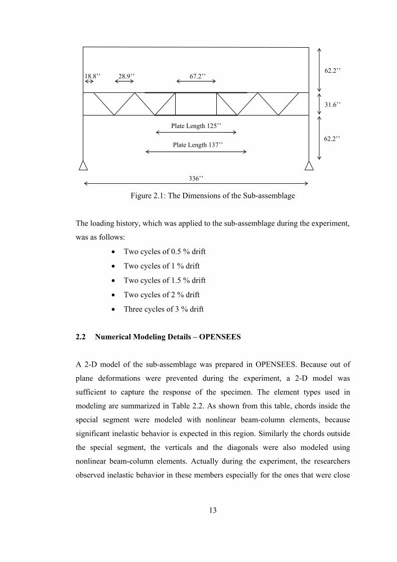
Figure 2.1: The Dimensions of the Sub-assemblage .................................................. 13

Figure 2.2: Comparison of the Experimental Result with the Analytical Result

Obtained for 1% Hardening ....................................................................................... 16


Obtained for 5% Hardening ....................................................................................... 16


Obtained for 10% Hardening ..................................................................................... 17

Figure 2.5: Details of Plastic Hinge Location ............................................................ 18

Figure 2.6: Comparison of Experimental Result with Numerical Result Obtained for

Reduced Special Segment Length .............................................................................. 18

Figure 2.7: Typical Finite Element Mesh .................................................................. 19

Figure 2.8: Comparison of Experimental Result with Finite Element Analysis Result

.................................................................................................................................... 20

Figure 3.1: Geometrical Properties of the STMFs ..................................................... 23

Figure 3.2: Free Body Diagram – Same Strength in All Stories ................................ 24

Figure 3.3: Free Body Diagram – Shear Distribution from Elastic Analysis ............ 26

xii

Figure 3.4: Distribution of Shear Strength among the Stories (6 Story STMF) ........ 27

Figure 3.5: Distribution of Shear Strength among the Stories (9 Story STMF) ........ 27

Figure 3.6: Distribution of Shear Strength among the Stories (12 Story STMF) ...... 28

Figure 3.7: Pushover Analysis Results for 6 Story STMF – Top Loading ................ 29

Figure 3.8: Pushover Analysis Results for 6 Story STMF – Equal Lateral Loading .....

.................................................................................................................................... 30

Figure 3.9: Pushover Analysis Results for 6 Story STMF – Inverted Triangular

Loading ...................................................................................................................... 30

Figure 3.10: Pushover Analysis Results for 6 Story STMF – CGL Loading ............ 31

Figure 3.11: Pushover Analysis Results for 9 Story STMF – Top Loading .............. 31

Figure 3.12: Pushover Analysis Results for 9 Story STMF – Equal Lateral Loading ...

.................................................................................................................................... 32


Loading ...................................................................................................................... 32

Figure 3.14: Pushover Analysis Results for 9 Story STMF – CGL Loading ............ 33

Figure 3.15: Pushover Analysis Results for 12 Story STMF – Top Loading ............ 33

Figure 3.16: Pushover Analysis Results for 12 Story STMF – Equal Lateral Loading

.................................................................................................................................... 34


Loading ...................................................................................................................... 34

Figure 3.18: Pushover Analysis Results for 12 Story STMF – CGL Loading .......... 35

Figure 3.19: Response Spectra for the Selected Earthquake Records ....................... 36

Figure 3.20: Comparison of Pushover and Time-History Analysis Results for 6 Story

STMF-PD ................................................................................................................... 38


STMF-ED-IT ............................................................................................................. 39


STMF-ED-CGL ......................................................................................................... 39


STMF-PD ................................................................................................................... 40

xiii


STMF-ED-IT ............................................................................................................. 40


STMF-ED-CGL ......................................................................................................... 41

Figure 3.26: Comparison of Pushover and Time-History Analysis Results for 12

Story STMF-PD ......................................................................................................... 41


Story STMF-ED-IT .................................................................................................... 42


Story STMF-ED-CGL ................................................................................................ 42

Figure 3.29: Response of 6 Story STMF-PD ............................................................. 43

Figure 3.30: Response of 6 Story STMF-ED-IT ........................................................ 44

Figure 3.31: Response of 6 Story STMF- ED-CGL .................................................. 44

Figure 3.32: Response of 9 Story STMF-PD ............................................................. 45

Figure 3.33: Response of 9 Story STMF-ED-IT ........................................................ 45

Figure 3.34: Response of 9 Story STMF-ED-CGL ................................................... 46

Figure 3.35: Response of 12 Story STMF-PD ........................................................... 46

Figure 3.36: Response of 12 Story STMF-ED-IT ...................................................... 47

Figure 3.37: Response of 12 Story STMF-ED-CGL ................................................. 47

Figure 3.38: Comparisons of Different Designs – 6 Story Systems .......................... 48

Figure 3.39: Comparisons of Different Designs – 9 Story Systems .......................... 49

Figure 3.40: Comparisons of Different Designs – 12 Story Systems ........................ 49

Figure 3.41: Ratio of Response Quantities – 6 Story Systems .................................. 50

Figure 3.42: Ratio of Response Quantities – 9 Story Systems .................................. 51

Figure 3.43: Ratio of Response Quantities – 12 Story Systems ................................ 51

Figure 4.1: Dimensions of the Numerical Model ...................................................... 57

Figure 4.2: The Normalized Moment Values versus Lateral Drift for A572-Gr50

Type of Steel .............................................................................................................. 62

Figure 4.3: The Normalized Moment Values versus Lateral Drift for A36 Type of

Steel ............................................................................................................................ 62

xiv

Figure 4.4: Ratio of Predicted to the Results of Analysis for Systems with A36 Type

of Steel – 2m Ls .......................................................................................................... 71


of Steel – 2.5m Ls ....................................................................................................... 71


of Steel – 3m Ls .......................................................................................................... 72

Figure 4.7: Ratio of Predicted to the Results of Analysis for Systems with A572-

Gr50 Type of Steel – 2m Ls ....................................................................................... 72


Gr50 Type of Steel – 2.5m Ls .................................................................................... 73


Gr50 Type of Steel – 3m Ls ....................................................................................... 73

Figure 5.1: Geometrical Properties of the Systems .................................................... 76

Figure 5.2: Pushover Analysis Results for Systems Having X-Diagonals with Zero

Slenderness ................................................................................................................. 80

Figure 5.3: Pushover Analysis Results for Systems Having X-Diagonals with Infinite

Slenderness ................................................................................................................. 80

Figure 5.4: Cyclic Pushover Analysis Results for Systems Having X-Diagonals with

Zero Slenderness ........................................................................................................ 81


Infinite Slenderness .................................................................................................... 82

Figure 5.6: Average Normalized Curvature Values for Different Design Types ...... 84

Figure 5.7: Average Normalized Axial Strain Values for Different Design Types ... 85

Figure 5.8: Average Base Shear Values for Different Design Types ........................ 85

Figure 5.9: Average Lateral Drift Values for Different Design Types ...................... 86

1

CHAPTER 1

1INTRODUCTION

1.1 Description of Special Truss Moment Frames (STMFs)

Special Truss Moment Frames (STMFs) can be used as a seismic load resisting

system in buildings. STMFs can be thought of as a combination of moment resisting

frames and eccentrically braced frames. In a typical STMF, girders are composed of

trusses which have a weak special segment near the mid-span as shown in Figure 1.1.

Figure 1.1: Typical Special Truss Moment Frames

2

The truss consists of top and bottom chord members, verticals, and diagonals. Like

the eccentrically braced frames, a weak link called the special segment, is present in

all STMFs. This weak region can be in the form of a vierendeel segment or a

vierendeel with X-braces. The idea is that when earthquake forces act on the

structure, high shear forces will develop at the mid-span of the truss leading to

yielding in this region. For the vierendeel type systems plastic hinges form at the top

and bottom chord ends. On the other hand, for vierendeel with X-braces, the braces

yield under tension and buckle under compression, while plastic hinges form at the

chord ends. A typical yielding mechanism for STMFs is given in Figure 1.2.

Figure 1.2: Yielding Mechanism for STMFs

There are various advantages of using STMF systems which can be summarized as

follows:

• These systems require simple details for moment connections.

• These systems are more economical than solid web beam frames

• Being lighter the truss girders can be used for longer spans.

• These systems have greater overall structural stiffness due to deeper girders

• Web openings can be used for piping and duct work as shown in Figure 1.3.

3

Figure 1.3: STMF with Piping and Duct Work

There are design provisions for STMFs presented in the AISC Seismic Provisions for

Steel Buildings. Unfortunately, no code provisions exist in Eurocodes. The

development of STMFs is attributable to Professor Goel at The University of

Michigan and his colleagues. The STMF system is relatively new and quite a few

buildings in the United States utilize this type of framing as shown in Figure 1.4.

Figure 1.4: A Real Application of STMF

The following sections outline the research work conducted to date in chronological

order to demonstrate the development of these systems.

4

1.2 Past Research on STMFs

Goel and Itani (1994a)

This is the first paper published on STMFs. The authors aimed to develop an open-

web truss-moment frame in this research. A prototype building was selected and

designed according to 1988 UBC requirements. Based on the design, a total of three

full-scale half-span truss column sub-assemblages were tested under large reversed

cyclic displacements. The truss girders had single diagonal members. Under cyclic

loading these single diagonals buckled and yielded. Because there was a single

diagonal at each panel, the load carrying capacity decreased significantly after

buckling. Representative load displacement diagram is given in Figure 1.5.

Apart from the experimental studies, the authors also conducted numerical analysis

to investigate the earthquake performance of single diagonal systems. The authors

concluded that the hysteretic behavior under cyclic loading is very poor because of

buckling and early fracture of truss web members. In addition, the inelastic dynamic

response analysis showed that such systems respond poorly to severe ground motions

with large story drifts and excessive inelastic deformations of truss web members

and columns.

Goel and Itani (1994b)

In a companion paper, the authors investigated the potential of using an X-diagonal

system for STMFs. After observing the poor behavior of single diagonals the authors

decided to use an X-type system. This way when one of the diagonals buckles under

compression the other diagonal is under tension and should be capable of carrying

the shear forces. A one story sub-assemblage consisting of a full-span truss and two

columns at the ends was tested. Two sub-assemblages were tested and the difference

was the applied displacement protocol. In general, the specimens showed stable

behavior. A representative load displacement behavior is given in Figure 1.6.

The authors conducted time-history analysis to investigate the performance of truss

girders with X-type diagonals. The findings of this research showed that the

5

proposed system can be an excellent and efficient seismic resistant framing system

for certain classes of building structures.

Figure 1.5: A Typical Load-Displacement Response for an STMF with Single Diagonals (Goel and Itani, 1994a)

Figure 1.6: A Typical Load-Displacement Response for an STMF with X-type Diagonals (Goel and Itani, 1994b)

Basha and

The autho

energy. Th

on using d

space. In t

of the spe

a set of nu

In the exp

A represen

was condu

one-bay su

the sub-as

displacem

was tested

revealed th

1.7.

Figure 1

d Goel (199

ors investig

he previous

diagonals in

this study, a

cial segmen

umerical ana

perimental p

ntative floo

ucted accord

ub-assembl

ssemblage w

ment historie

d under the

hat the sub-

.7: A Typic

94)

gated the po

s research w

n the special

a vierendee

nt. The wor

alysis.

program ST

or plan was

ding to 199

lage of a typ

was first te

es were app

presence o

-assemblage

cal Load-DiSegme

6

otential use

work by Go

l segment. T

el panel was

rk consisted

TMFs with a

selected for

1 UBC prov

pical story

ested witho

plied. Afterw

of point load

e provide st

splacement ent (Basha a

e of a viere

oel and Itan

These diago

s proposed

d of an expe

and without

r a 4-story b

visions. Ba

was experi

ut the appl

wards the s

ds that simu

table hyster

Response fand Goel, 1

endeel segm

ni (1994a, 1

onals may r

as an altern

erimental pr

t gravity loa

building an

sed on the d

mented. As

lication of

ame kind o

ulate gravit

retic behavi

for an STM994)

ment for dis

994b) conc

restrict the a

native confi

rogram follo

ading were

nd the STMF

designed se

s mentioned

gravity loa

of a sub-ass

ty loading.

ior as shown

MF with Vier

ssipating

centrated

available

iguration

owed by

studied.

F design

ctions, a

d before,

ds. Two

emblage

All tests

n in Fig.

rendeel

7

A detailed investigation of the specimen behavior is presented in Chapter 2.

Therefore, the specimen details are presented later.

The authors concluded that the responses of the sub-assemblages under lateral loads

alone as well as under combined gravity and lateral loads were full and stable with

no pinching and degradation. A set of modeling recommendations were presented

for systems with a vierendeel segment. The dynamic response from numerical

studies was excellent.

Goel, Rai, and Basha (1998)

In this research report the authors present guidelines for the design of STMFs. The

limit state design philosophy applied to STMFs was presented. The special segment

of the STMF is expected to yield and dissipate energy, while the rest of the system

remains elastic. Only yielding at the column bases is permitted. In this guide several

rules based on limit state design were given to proportion the truss members that are

outside the special segment. Design of STMFs with vierendeel segment and with X-

bracing was explained by making use of examples. Both hand calculations and

computer analysis were given. After presenting the design of the STMFs authors

presented some analytical results on these representative designs. Basically, pushover

analysis and nonlinear time history analysis were conducted to investigate the

performance of these systems. The report concluded with a short set of design

recommendations that was adopted by the 1997 UBC specification.

Parra-Montesinos, Goel, and Kim (2006)

In this research the authors studied the performance of steel double-channel built-up

chords of STMF. Rather than experimenting the whole system, the researchers

concentrated on the chord members. Back-to-back channel sections may be used to

increase the base shear capacity for STMF with a vierendeel segment. In this

experimental program, six cantilever double-channel members were subjected to

reverse cyclic loading to observe their performance. The main parameters were the

stitch spacing and lateral bracing for the channel members. The authors concluded

that the current AISC requirements for stitch spacing and lateral bracing are not

8

adequate to ensure large rotation capacity in double channel built-up members. A

new equation was proposed based on the test results.

Chao and Goel (2008a)

The primary goal of the researchers was to propose a modified expression for the

expected shear strength of the special segment. Members outside of the special

segment were proportioned using capacity design principles and the applied loads

were derived based on the shear strength of the special segment. Over the years, Goel

and his colleagues developed expressions for the expected shear strength and their

developments lead to the code provisions. These expressions take into account the

formation of plastic hinges at the chord ends, yielding of diagonals in tension,

buckling of diagonals in compression, flexibility of chord members and etc. Chao

and Goel identified that the expected shear strength expression presented in the AISC

specification may lead to overdesign of the members if the moment of inertia of the

member is large. In order to develop a modified expression, the authors conducted a

set of nonlinear static and dynamic analyses. Based on the analyses results the

authors concluded that the AISC equation significantly overestimates the expected

shear strength. Based on the findings of the numerical analysis a more refined

expression was developed.

Chao and Goel (2008b)

In this research, the authors developed a performance based plastic design

methodology for STMFs. Before this research work, the STMFs were designed using

elastic analysis methods. The use of elastic analysis to proportion the members lead

to nonuniform distributions of story drifts and yielding in special segments along the

height of the structure. In order to achieve a more uniform yielding and story drifts

the authors developed a design methodology. The performance based plastic design

approach is based on energy theorems and does not require the use of a response

modification factor. The procedure is performance based, therefore, the target drift

has to be known or determined in advance. The authors derived an expression for a

modified base shear, based on energy concepts. The modified base shear is

dependent on the target drift, preselected yield mechanism, and code-specified elastic

9

design spectral value for a given hazard level. The modified base shear actually

corresponds to the base shear at the structural collapse level. Therefore, this base

shear value can be directly used in the plastic design of the structure. The code

specified base shear value is generally less than the modified base shear, and

corresponds to the level at the first significant yield. The procedure uses a lateral load

profile that was developed by Chao, Goel, and Lee (2007). This lateral load profile

was developed based on different steel structural systems such as moment frames,

concentrically braced frames, eccentrically braced frame, and STMFs.

The authors verified the proposed performance based design approach by a 9-story

STMF subjected to SAC ground motions. The analysis results revealed that the

design based on the proposed methodology resulted in uniform interstory drifts. In

addition, the maximum amount of drift was less than the target value.

AISC Code Provisions for STMFs

AISC Seismic Provisions for Structural Steel Buildings (2005) provide a few rules

for the design of STMFs. The span length and depth of the truss is limited to 20m

and 1.8m, respectively. Columns and truss segment outside the special segment

should be designed to remain elastic during a seismic event. The length of the special

segment should be between 0.1 to 0.5 times the truss span length. The length to depth

ratio of the special segment should be kept between 1.5 and 0.67. The special

segment can contain vierendeel panels or X-braced panels. For X-braced panels the

bracing can be from flat bars that are connected at the intersection of braces.

The shear strength of the special segment shall be calculated as the sum of the

available shear strength of the chord members through flexure, and the shear strength

corresponding to the available tensile strength and 0.3 times the available

compressive strength of the diagonal members, when they are used. The shear

strength (Vn) can be calculated as follows according to the AISC definition:

αsin)3.0(4

ncnts

ncn PP

LM

V ++= Equation (1.1)

10

Where;

Mnc: nominal flexural strength of a chord member of the special segment

Ls: length of the special segment

Pnt: nominal tensile strength of a diagonal member of the special segment

Pnc: nominal compressive strength of a diagonal member of the special segment

α: angle of diagonal members with the horizontal.

For special segments with X-bracing, the top and bottom chord members shall

provide at least 25 percent of the required vertical shear strength.

Strength of non-special segment members shall be determined from capacity design.

The AISC Specification provides the following equation for calculating the expected

shear strength of the special segment (Vne):

αsin)3.0()(

075.075.3

3 ncntys

s

s

ncyne PPR

LLL

EIL

MRV ++

−+= Equation (1.2)

Where;

EI: flexural elastic stiffness of a chord member of the special segment

L: span length of the truss

Ry: ratio of the expected yield stress to the specified minimum yield stress.

Once the expected strength of the special segment is calculated from Equation 1.2,

then forces on the columns and truss members outside the special segment can be

calculated using this maximum amount of shear produced. The Equation 1.2 takes

into account the increased moments at the chord member ends due to the strain

hardening. In addition, the material overstrength is accounted for using the Ry factor.

Recent research conducted by Chao and Goel (2008a) showed that Equation 1.2

provides overestimates of the expected shear strength. Authors proposed an

alternative equation for replacement of the code equation.

11

AISC Specification mandates that the chord members and diagonal web members

within the special segment must be seismically compact. In addition, lateral bracing

should be provided at both ends of the top and bottom chord members.

1.3 Scope of the Thesis

The thesis work consists of a three phase numerical study on STMFs. In the first

phase the design philosophy for multistory STMFs were evaluated. The distribution

of shear strength among the stories was studied through dynamic time-history

analyses. In the second phase, the expected shear strength formulations for

vierendeel segment were evaluated. The expected shear strength was studied through

detailed three dimensional finite element models of one story STMFs. In the third

phase the effect of load share between chord members and X-diagonals were studied

taking into account different diagonal slenderness values. Time-history analyses

were conducted to evaluate the response of single story systems in phase three.

The numerical analyses for phase 1 and 3 were conducted using OPENSEES while

the finite element calculations were performed using ANSYS. In Chapter 2, the

numerical models were verified against the experimental results. The details of the

studies and results of phases 1, 2, and 3 are given in Chapters 3, 4, and 5,

respectively. Finally, the conclusions are presented in Chapter 6.

12

CHAPTER 2

2MODELING ASSUMPTIONS AND VERIFICATION OF OPENSEES AND ANSYS SOFTWARE

The verification of software was conducted by utilizing the experimental results

presented by Basha and Goel (1994). Only STMFs with a vierendeel segment is

treated herein.

2.1 Details of the Experimental Setup

Basha and Goel (1994) conducted quasi-static experiments on a sub-assemblage as

shown in Figure 2.1. In this setup, lateral loading was applied to one of the columns

using a hydraulic actuator. A link beam with pinned ends was connected to the

column tops to transfer this lateral load to both columns. The specimen consisted of a

truss member with a vierendeel segment. The sizes of the members are summarized

in Table 2.1. All angles were A572 steel with a nominal yield strength of 50 ksi. The

measured yield strength from coupon tests ranged between 60 to 63 ksi. All

sandwich plates were A36 steel with a nominal yield strength of 36 ksi. The

measured yield strength from coupon tests was 48 ksi. The sandwich plates were

welded between the angles and were extended beyond the special segment to provide

the development length of the built-up section.

Table 2.1: Section Properties of the Members

Member Section Fy ksi

Chords within the Special Segment 2L 3x3x1/2 PL 2-1/4x1

50 36

Chords outside the Special Segment 2L 3x3x1/2 50 Diagonals 2L 2-1/2x2-1/2x1/4 50 Verticals 2L 1-1/2x1-1/2x1/4 50

13

Figure 2.1: The Dimensions of the Sub-assemblage

The loading history, which was applied to the sub-assemblage during the experiment,

was as follows:

• Two cycles of 0.5 % drift

• Two cycles of 1 % drift

• Two cycles of 1.5 % drift

• Two cycles of 2 % drift

• Three cycles of 3 % drift

2.2 Numerical Modeling Details – OPENSEES

A 2-D model of the sub-assemblage was prepared in OPENSEES. Because out of

plane deformations were prevented during the experiment, a 2-D model was

sufficient to capture the response of the specimen. The element types used in

modeling are summarized in Table 2.2. As shown from this table, chords inside the

special segment were modeled with nonlinear beam-column elements, because

significant inelastic behavior is expected in this region. Similarly the chords outside

the special segment, the verticals and the diagonals were also modeled using

nonlinear beam-column elements. Actually during the experiment, the researchers

observed inelastic behavior in these members especially for the ones that were close

62.2’’

62.2’’

31.6’’

18.8’’ 28.9’’ 67.2’’

336’’

Plate Length 137’’

Plate Length 125’’

14

to the special segment. Actual yield strengths and the dimensions presented in

Figure 2.1 were used in modeling. The link beam was modeled using a truss element

and columns were modeled using elastic beam-column elements.

Table 2.2: Element Types of the Members

All cross sections were modeled using fiber elements. The nonlinear material

behavior of steel was modeled using a built-in material model named “steel02”. This

material model is well suited for cyclic behavior of steel and accounts for the

Bauschinger effect.

In the previous analytical studies conducted by Basha and Goel (1994), researchers

used a lumped plasticity element to model the special segment chord members. This

element requires the moment versus rotation behavior of plastic hinges at the

member ends. Basha and Goel (1994) stated that the customary moment rotation

relationships used for moment resisting frames are not suitable for modeling the

STMFs. The key point here is the selection of a post yield slope to represent the

strain hardening effects. In general a post yield slope of 5% is used for representing

the moment rotation response for typical members in moment resisting frames.

Basha and Goel (1994) have identified that using a 5% slope is inadequate for

modeling the STMFs. Because the special segment lengths are rather short in these

kinds of systems, the curvature and rotation demands are significantly different. By

using a trial and error procedure, Basha and Goel (1994) concluded that using a 10%

post yield slope is sufficient for modeling purposes.

Member Element Chords within the Special Segment nonlinearBeamColumn Element Chords outside the Special Segment nonlinearBeamColumn Element

Diagonals nonlinearBeamColumn Element

Verticals nonlinearBeamColumn Element

Columns elasticBeamColumn Element

Link Beam truss Element

15

The modeling technique adopted in this thesis is different than the one of Basha and

Goel (1994). The nonlinear beam-column element, used in modeling the chord

members, was combined with fiber sections to model the cross section behavior. The

element requires inputting a material stress-strain law to convert the stresses to stress

resultants. Therefore, an explicit moment-rotation behavior is not needed in these

kinds of elements. The strain hardening behavior is treated at the material level by

changing the hardening modulus value.

In order to calibrate the numerical model with the experimental results, three

different hardening modulus values were considered in this study. These modulus

values represent 1%, 5%, and 10% of the elastic modulus of steel.

2.2.1 Analysis Results

The load displacement responses obtained using the OPENSEES software, were

compared with the experimental results in Figures 2.2, 2.3, and 2.4. According to the

comparisons, numerical modeling with a hardening modulus of 5% of the elastic

modulus gives the best result among the three. The maximum amount of lateral load

measured during testing was 58 kips. The maximum amount of lateral load from

numerical analysis was 56.5 kips using a 5% post yield slope. Moreover, in all cases

the elastic stiffness from the simulations was 20 kips/in which is identical to the

experimentally observed value.

Although using a hardening modulus of 5% of the initial elastic modulus gives

promising results, this assumption is not consistent with real observations on material

behavior. Usually the hardening modulus from cyclic material tests ranges between

0.5 and 1 percent of the initial elastic modulus. Therefore, using 5% of the initial

modulus is unrealistic and can have adverse effects on the analysis results. In fact

preliminary analysis using a 5 percent slope showed significant amount of hardening

for these systems. Because of these reasons, additional verification studies were

conducted in this thesis to better simulate the system by using realistic hardening

values.

16

Figure 2.2: Comparison of the Experimental Result with the Analytical Result Obtained for 1% Hardening


-80

-60

-40

-20

0

20

40

60

80

-4 -3 -2 -1 0 1 2 3 4

Lat

eral

Loa

d, k

ips

Lateral Drift, %

Experiment OPENSEES

-80

-60

-40

-20

0

20

40

60

80

-4 -3 -2 -1 0 1 2 3 4

Lat

eral

Loa

d, k

ips

Lateral Drift, %

Experiment OPENSEES

17


A careful examination of the truss geometry as depicted by Basha and Goel (1994)

indicated that the length of the special segment is 67.2 inches. This value

corresponds to the distance between the centerlines of the two verticals that were

placed at both ends of the chord members. A more accurate computer model should

consider the clear distance between the verticals. In addition, during the formulation

of the beam-column elements the integration is carried at the ends and these are the

locations where the plastic hinges occur. In reality, however, plastic hinges penetrate

into the member and can form further away from the ends. Usually the plastic hinges

can form at a distance between half of the member depth to a full member depth.

Taking these into account, a revised length equal to 61.2 inches was used in the

computer modeling. As shown in Figure 2.5, this length was obtained by considering

the clear distance between the verticals (i.e. subtracting the depth of verticals for the

centerline distance value) and assuming that the plastic hinges will form at a distance

equal to half of the chord member depth.

-80

-60

-40

-20

0

20

40

60

80

-4 -3 -2 -1 0 1 2 3 4

Lat

eral

Loa

d, k

ips

Lateral Drift, %

Experiment OPENSEES

18

Figure 2.5: Details of Plastic Hinge Location

The same analysis was conducted using this reduced length for the special segment

and utilizing a hardening modulus equal to 1 percent of the initial elastic modulus.

The result is presented in Figure 2.6.

Figure 2.6: Comparison of Experimental Result with Numerical Result Obtained for

Reduced Special Segment Length

-80

-60

-40

-20

0

20

40

60

80

-4 -3 -2 -1 0 1 2 3 4

Lat

eral

Loa

d, k

ips

Lateral Drift, %

Experiment OPENSEES

Top Chord

Vertical

dvertical

dchord/2

Plastic Hinge

19

According to the revised result it is evident that considering a reduced length with

more realistic material properties was sufficient to capture the response. The use of a

hardening modulus equivalent to 1 percent of the initial elastic modulus will be

further justified in the following section on finite element analysis.

2.3 Numerical Modeling Details – ANSYS

A full three dimensional model of the specimen was prepared in ANSYS. All

elements were modeled using 8-node shell elements (shell93). The link beam was

modeled with truss elements (link8). Bilinear kinematic hardening with a slope of 1

percent of the initial elastic slope was utilized in the model. The same displacement

history utilized in testing was applied to the model. The chord member ends were

finely meshed to adequately model the inelastic behavior in these regions. A typical

finite element mesh is given in Figure 2.7.

Figure 2.7: Typical Finite Element Mesh

20

The finite element model of the specimen was modeled using 192 nodes and 132

shell elements. The chord members were meshed into two in coarsely meshed

regions and into six in finely meshed regions.

The comparison of load displacement response from the experimental result and

numerical result is given in Figure 2.8. It is evident from the comparison that the

finite element simulation is satisfactory in predicting the response of the specimen.

Figure 2.8: Comparison of Experimental Result with Finite Element Analysis Result

Simulations utilizing OPENSEES and ANSYS revealed that the specimen behavior

can be predicted with reasonable level of accuracy using these software. Further

numerical studies presented in this thesis employed the numerical details adopted in

this chapter.

-80

-60

-40

-20

0

20

40

60

80

-4 -3 -2 -1 0 1 2 3 4

Lat

eral

Loa

d, k

ips

Lateral Drift, %

Experiment ANSYS

21

CHAPTER 3

3AN EVALUATION OF STRENGTH DISTRIBUTION IN STMFs

Design of STMF systems presents a variety of challenges especially for earthquake

loads. Engineers frequently utilize equivalent static load procedures to take into

account the inertia forces produced during an earthquake. Regardless of the

specification used and its recommended lateral load distribution, the problem of

designing for strength at each story level arises. Engineers have options for the

distribution of shear strength of special segment among the stories. First studies

(Goel and Itani (1994b)) on design of STMFs recommended the use of same truss at

all story levels leading to an equal distribution of shear strength among the stories.

Some earlier studies suggested that the truss members can be sized based on the

elastic shear force distribution. Recently, Chao and Goel (2008b) recommended that

a special lateral force distribution developed by Chao, Goel, and Lee (2007) should

be used in the design of STMF systems and the sizing should be based on the elastic

shear forces produced by this lateral load distribution.

The lateral load distribution proposed by Chao, Goel, and Lee (2007) is calculated as

follows:

( ) 0 , 11 ==−= ++ nniii niwhenFF βββ

2.075.0

1

−

⎟⎟⎟⎟⎟

⎠

⎞

⎜⎜⎜⎜⎜

⎝

⎛

=

∑=

T

n

jjj

nnn

hw

hwVF Equation (3.1)

22

2.075.0 −

⎟⎟⎟⎟⎟

⎠

⎞

⎜⎜⎜⎜⎜

⎝

⎛

==∑=

T

nn

n

ijjj

n

ii hw

hw

VV

β Equation (3.2)

Where;

βi: shear distribution factor at level i

Vi, Vn: story shear forces at level i and at the top (nth level), respectively

wj: seismic weight at level j

hj: height of level j from the ground

wn: seismic weight of the structure at the top level

hn: height of roof level from the ground

T: fundamental natural period

Fi, Fn: lateral forces applied at level i and top level n, respectively

V: design base shear.

This lateral load distribution takes into account the higher amounts of forces

produced at top stories during an earthquake. Chao and Goel (2008b) proposed a

performance based design methodology for STMFs that is based on this lateral load

distribution and a target interstory drift level. These researchers concluded that the

lateral drift and plastic rotation demands tend to be uniform if the proposed design

methodology is adopted.

The aim of the study presented in this chapter is to explore the seismic behavior of

STMFs designed using different lateral load distributions and special segment

strength variations among the stories. The main objective of the study is to quantify

the consequences of using same truss designs in all stories. This design philosophy is

useful because it expedites the design and manufacturing of STMFs. Only a single

type of truss needs to be designed and manufactured in this case. If a design based on

elastic analysis is considered then several different truss designs should be conducted

and the manufacturing should accommodate these different designs.

23

3.1 Methodology and Design of STMFs

In order to compare different designs and load distributions 6, 9, and 12 story STMFs

with a vierendeel segment were considered. A single story portion of a typical STMF

is given in Figure 3.1. As shown in this figure, a column height of 2.5m, a truss depth

of 1m, a span length of 10m, and a special segment length of 2m were considered.

Figure 3.1: Geometrical Properties of the STMFs

In order to make a fair comparison between the designs, same sections were used for

the members outside the special segment, in all cases. All members outside the

special segment were modeled to behave elastically during the analysis and plastic

behavior was constrained to the chord members in special segment. If the engineer

chooses to utilize same section members in all stories then the strength is equally

distributed along the height of the STMF as shown in Figure 3.2. In this type of a

design, the distribution of lateral forces only has an influence on the sum of the shear

strengths in all stories.

10m

2m

1m

2.5m

Special Segment

24

The relationship between the required strength of the special segment (Vss) and the

base shear (Vlateral) can be expressed as:

nLHV

V eqlateralss = Equation (3.3)

Where;

Heq: equivalent height of the applied lateral load

n: number of stories.

Figure 3.2: Free Body Diagram – Same Strength in All Stories

Vss

L/2

Heq

Vlateral

Vlateral/2 Vlateral/2

L/2

Vss

Vss

Vss

Vss

Vss

L/2

Heq

Vlateral


L/2

Vss

Vss

Vss

Vss

25

In the present study two C10x15.3 channel section chord members with a yield

strength of 350 MPa were considered for the truss with same strength sections in all

stories. The rest of the truss system was designed based on the strength of the special

segment. The panel length for all trusses was 1m. The sections used for the members

outside the special segment are given in Table 3.1.

Table 3.1: Members outside the Special Segment Member Section

Chord outside the Special Segment 2MC18x58 Diagonals 2L5x5x1/2 Verticals 2L4x4x7/16 Columns W36x652

The sum of shear strengths of the special segments with 2C10x15.3 sections are

equal to 2184kN, 3276kN, 4368kN for 6, 9, and 12 story STMFs, respectively.

These strength values were kept constant and distributed according to the elastic load

share of each story produced by a particular lateral load distribution. As shown in

Figure 3.3, the distribution of the shear forces on the special segments varies if the

design is based on elastic analysis. In order to keep the shear strength values the

same, the following condition was applied:

∑=n

ississ VnV Equation (3.4)

Where;

Vssi: shear on special segment at the ith level

Based on the elastic distribution of forces and the total shear strength requirement,

the shear forces on special segments were determined. By considering these forces

the chord members of the special segment were designed for lateral forces that

correspond to inverted triangular distribution and Chao, Goel, and Lee (2007)

distribution which is referred as CGL distribution hereafter.

26

Figure 3.3: Free Body Diagram – Shear Distribution from Elastic Analysis

The design, where all trusses along the building height were the same, is termed as

plastic design (PD). The design, where the trusses were designed based on elastic

force distribution, is termed as elastic design (ED). There are two types of elastic

design that was conducted namely, design based on inverted triangular distribution

(ED-IT) and design based on CGL distribution (ED-CGL).

The required strength normalized by the total shear strength of all segments are

plotted as a function of story number in Figures 3.4, 3.5, and 3.6 for 6, 9, and 12

story STMFs, respectively. The designed sections for each analysis or loading case

are given in Table 3.2.

Vss5

L/2

Heq

Vlateral


L/2

Vss4

Vss3

Vss2

Vss1

Vss5

L/2

Heq

Vlateral


L/2

Vss4

Vss3

Vss2

Vss1

27

Figure 3.4: Distribution of Shear Strength among the Stories (6 Story STMF)


0

1

2

3

4

5

6

7

0 0.05 0.1 0.15 0.2 0.25

Stor

y N

umbe

r

Special Segment Shear Strength / Total Shear Strength

IT CGL PD ED-IT ED-CGL

0

1

2

3

4

5

6

7

8

9

10

0 0.05 0.1 0.15 0.2

Stor

y N

umbe

r



28


Table 3.2: Chord Member Sections Six Story Nine Story Twelve Story

Story Number

Inverted Triangular CGL Inverted

Triangular CGL Inverted Triangular CGL

1 2C10x25 2C10x25 2C10x25 2C10x25 2C10x25 2C10x25 2 2C10x25 2C10x20 2C10x25 2C10x25 2C10x25 2C10x25 3 2C10x20 2C10x20 2C10x25 2C10x20 2C10x25 2C10x25 4 2C10x15.3 2C10x15.3 2C10x25 2C10x20 2C10x25 2C10x20 5 2C9x13.4 2C9x13.4 2C10x20 2C10x20 2C10x25 2C10x20 6 2C7x9.8 2C7x12.2 2C10x15.3 2C10x15.3 2C10x20 2C10x20 7 2C9x13.4 2C9x15 2C9x20 2C9x20 8 2C8x11.5 2C8x13.7 2C9x20 2C10x15.3 9 2C6x8.2 2C7x9.8 2C9x13.4 2C8x18.7

10 2C7x14.7 2C9x13.4 11 2C7x9.8 2C8x11.5 12 2C5x6.7 2C6x10.5

For dynamic analysis purposes it was assumed that the mass at every story is 125

tons. For all cases the members outside the special segment were kept the same in

order not to introduce other variables.

0

2

4

6

8

10

12

14

0 0.02 0.04 0.06 0.08 0.1 0.12 0.14

Stor

y N

umbe

r



29

3.2 Static Pushover Analysis and Natural Periods

In order to make sure that the different truss designs give similar base shear values, a

set of pushover analysis were conducted on the STMF systems. Basically four

different lateral load procedures were applied to obtain pushover responses. These

four load profiles include a point load at the topmost story, equal lateral load, CGL

load distribution, and inverted triangular load distribution. For all analyses a

hardening modulus of 1 GPa was considered. Figures 3.7 through 3.18 present the

findings of the pushover analysis results. As can be seen from these figures, the

responses of the three different designs are similar. Essentially for all loading types

the trusses designed using an elastic inverted triangular distribution and the CGL

distribution display very similar responses. The response of the truss designed based

on equal strength in all stories concept deviates slightly from the response of other

two for equal lateral and inverted triangular loadings.

Figure 3.7: Pushover Analysis Results for 6 Story STMF – Top Loading

0

200

400

600

800

1000

1200

1400

1600

0 0.5 1 1.5 2 2.5

Bas

e Sh

ear,

kN

Top Story Lateral Drift, %

PD ED-IT ED-CGL

30


Figure 3.9: Pushover Analysis Results for 6 Story STMF – Inverted Triangular Loading

0

500

1000

1500

2000

2500

3000

0 0.5 1 1.5 2 2.5

Bas

e Sh

ear,

kN


PD ED-IT ED-CGL

0

500

1000

1500

2000

2500

0 0.5 1 1.5 2 2.5

Bas

e Sh

ear,

kN


PD ED-IT ED-CGL

31

Figure 3.10: Pushover Analysis Results for 6 Story STMF – CGL Loading


0

500

1000

1500

2000

2500

0 0.5 1 1.5 2 2.5

Bas

e Sh

ear,

kN


PD ED-IT ED-CGL

0

200

400

600

800

1000

1200

1400

1600

0 0.5 1 1.5 2 2.5

Bas

e Sh

ear,

kN


PD ED-IT ED-CGL

32



Loading

0

500

1000

1500

2000

2500

3000

0 0.5 1 1.5 2 2.5

Bas

e Sh

ear,

kN


PD ED-IT ED-CGL

0

500

1000

1500

2000

2500

0 0.5 1 1.5 2 2.5

Bas

e Sh

ear,

kN


PD ED-IT ED-CGL

33



0

500

1000

1500

2000

2500

0 0.5 1 1.5 2 2.5

Bas

e Sh

ear,

kN


PD ED-IT ED-CGL

0

200

400

600

800

1000

1200

1400

1600

0 0.5 1 1.5 2 2.5

Bas

e Sh

ear,

kN


PD ED-IT ED-CGL

34



Loading

0

500

1000

1500

2000

2500

3000

0 0.5 1 1.5 2 2.5

Bas

e Sh

ear,

kN


PD ED-IT ED-CGL

0

500

1000

1500

2000

2500

0 0.5 1 1.5 2 2.5

Bas

e Sh

ear,

kN


PD ED-IT ED-CGL

35


Apart from pushover analysis, an eigenvalue analysis was conducted for each STMF

to obtain the natural periods of the systems. Natural periods for the first three modes

of vibration are given in Table 3.3. As shown in this table for a particular number of

story, the fundamental natural periods of STMFs designed using different methods

are close to each other.

Table 3.3: Natural Periods of STMF Systems

Number of Story

Period (sec) 1st Mode 2nd Mode 3rd Mode

Plastic Design

Elastic Design

(IT)

Elastic Design (CGL)

Plastic Design

Elastic Design

(IT)


Plastic Design

Elastic Design

(IT)


6 1.16 1.15 1.15 0.28 0.29 0.29 0.11 0.12 0.12 9 1.71 1.69 1.69 0.47 0.49 0.48 0.21 0.22 0.22

12 2.29 2.26 2.26 0.67 0.71 0.69 0.32 0.34 0.33

0

500

1000

1500

2000

2500

0 0.5 1 1.5 2 2.5

Bas

e Sh

ear,

kN


PD ED-IT ED-CGL

36

3.3 Time-History Analysis

A set of time-history analysis was conducted to study the behavior of STMFs under

earthquake loading. All structures were subjected to a suite of ground motions that

are listed in Table 3.4. These ground motions have a wide range of intensity and in

general, force the STMF behavior into the inelastic range. Earthquake records with

varying intensity were expected to produce different levels of drift demands so that

the behavior of STMFs at various drift levels can be examined. For all structures a

design base acceleration (DBA) was calculated by dividing the base shear at

structural yield level to the total reactive mass. The 2% damped response spectra of

the selected earthquakes and design base accelerations (DBAs) for 6, 9, and 12 story

systems are given in Figure 3.19.

Figure 3.19: Response Spectra for the Selected Earthquake Records

0

1

2

3

4

5

6

7

8

0 0.5 1 1.5 2 2.5 3

Sa, g

Period, sec.

2% Damped Response Spectragm1gm2gm3gm4gm5gm6gm7gm8gm9gm10gm11gm12gm13gm14gm15gm16gm17gm18gm19gm20DBA

37

Table 3.4: Details of Selected Ground Motion Records

GM # Earthquake Country Date Station Location Site

Geology Mw PGA (g)

1 Imperial Valley USA 15.10.1979 El Centro Array #1,

Borchard Ranch Alluvium 6.5 0.141

2 Morgan Hill USA 24.04.1984 Gilroy Array #2

(Hwy 101 & Bolsa Rd)

Alluvium 6.1 0.157

3 Northridge USA 17.01.1994 Downey County Maint. Bldg. Alluvium 6.7 0.223

4 Imperial Valley USA 15.10.1979 Meloland Overpass Alluvium 6.5 0.314

5 Northridge USA 17.01.1994 Saticoy Alluvium 6.7 0.368

6 Whittier Narrows USA 01.10.1987 Cedar Hill Nursery,

Tarzana Alluvium / Siltstone 6.1 0.405

7 Loma Prieta USA 18.10.1989 Capitola Fire Station Alluvium 7.0 0.472

8 Northridge USA 17.01.1994 Rinaldi Receiving Station Alluvium 6.7 0.480

9 Northridge USA 17.01.1994 Katherine Rd, Simi Valley Alluvium 6.7 0.513

10 Imperial Valley USA 15.10.1979 El Centro Array #5,

James Road Alluvium 6.5 0.550

11 Chi Chi Taiwan 20.09.1999 CHY028 USGS(C) 7.6 0.653

12 Cape Mendocino USA 25.04.1992 Petrolia, General

Store Alluvium 7.0 0.662

13 Kobe Japan 16.01.1995 Takarazu USGS (D) 6.9 0.693 14 Kobe Japan 16.01.1995 Takarazu USGS (D) 6.9 0.694

15 Northridge USA 17.01.1994 Katherine Rd, Simi Valley Alluvium 6.7 0.727

16 Düzce Turkey 12.11.1999 Bolu USGS(C) 7.1 0.754

17 Northridge USA 17.01.1994 Sepulveda VA Hospital Alluvium 6.7 0.939

18 Tabas Iran 16.09.1978 Tabas Stiff Soil _ 1.065 19 Morgan Hill USA 24.04.1984 Coyote Lake Dam Rock 6.1 1.298

20 Northridge USA 17.01.1994 Tarzana Cedar Hill Nursery Alluvium 6.7 1.778

All 9 STMF systems were subjected to the ground motions listed in Table 3.4. A

stiffness proportional damping equal to 2 percent of the critical damping was

considered in all analysis. During a typical analysis drifts at story levels, curvatures

at the chords of special segments, and the base shears were recorded. The curvature

values were converted to plastic rotations after analysis. The curvature-plastic

rotation relationship was derived by considering simple loading cases. A plastic

hinge length of 5 percent of the length of the member was obtained from Gauss-

Lobatto quadrature for five number of integration points. Taking into account this

38

plastic hinge length, a relationship between curvatures and plastic rotations can be

easily developed.

3.3.1 Results of Time-History Analysis

3.3.1.1 Comparison with Pushover Analysis

Time-history analysis results give useful information about the lateral loading profile

during a seismic event. In general many modes contribute to the response of a system

under dynamic loading. In this part of the study the time-history analysis results are

correlated with the pushover analysis results that were presented earlier. Basically,

the maximum absolute base shear and the maximum absolute top story drift were

considered for each 20 time-history analysis and these values are plotted against the

pushover curves obtained using different lateral load profile assumptions. The plots

are given in Figures 3.20 through 3.28.


STMF-PD

0

500

1000

1500

2000

2500

3000

3500

0 0.5 1 1.5 2 2.5

Bas

e Sh

ear,

kN


Top Triangular Equal Lateral CGL Dynamic

39


STMF-ED-IT


STMF-ED-CGL

0

500

1000

1500

2000

2500

3000

3500

0 0.5 1 1.5 2 2.5

Bas

e Sh

ear,

kN



0

500

1000

1500

2000

2500

3000

3500

0 0.5 1 1.5 2 2.5

Bas

e Sh

ear,

kN



40


STMF-PD


STMF-ED-IT

0

500

1000

1500

2000

2500

3000

0 0.5 1 1.5 2 2.5

Bas

e Sh

ear,

kN



0

500

1000

1500

2000

2500

3000

3500

0 0.5 1 1.5 2 2.5

Bas

e Sh

ear,

kN



41


STMF-ED-CGL


Story STMF-PD

0

500

1000

1500

2000

2500

3000

0 0.5 1 1.5 2 2.5

Bas

e Sh

ear,

kN



0

500

1000

1500

2000

2500

3000

0 0.5 1 1.5 2 2.5

Bas

e Sh

ear,

kN



42


Story STMF-ED-IT


Story STMF-ED-CGL

0

500

1000

1500

2000

2500

3000

3500

0 0.5 1 1.5 2 2.5

Bas

e Sh

ear,

kN



0

500

1000

1500

2000

2500

3000

3500

0 0.5 1 1.5 2 2.5

Bas

e Sh

ear,

kN



43

It is evident from these figures that most of the earthquake records result in an

inelastic activity in the systems. STMF systems remained elastic under the action of

a few of the ground motions. The comparisons with pushover analysis reveal that the

base shear versus top story drift can best be predicted using the equal lateral load

distribution. This observation is valid for all types of designs and all heights

considered.

3.3.1.2 Comparison of Different Designs

In this section the trusses designed based on three different approaches are compared

in terms of their performance. As mentioned earlier, two measures are used to

conduct the comparisons among the different designs. The maximum interstory drift

at all stories and the maximum amount of plastic rotation at the chord member ends

were recorded. For each STMF and 20 time-history analysis the results for these

quantities are given in Figures 3.29 through 3.37.

Figure 3.29: Response of 6 Story STMF-PD

0

1

2

3

4

5

6

7

0 1 2 3

Stor

y N

umbe

r

Maximum Interstory Drift, %

gm1gm2gm3gm4gm5gm6gm7gm8gm9gm10gm11gm12gm13gm14gm15gm16gm17gm18gm19gm20Mean

0

1

2

3

4

5

6

7

0 0.05 0.1

Stor

y N

umbe

r

Maximum Plastic Hinge Rotation, rad.


44

Figure 3.30: Response of 6 Story STMF-ED-IT

Figure 3.31: Response of 6 Story STMF- ED-CGL

0

1

2

3

4

5

6

7

0 1 2 3

Stor

y N

umbe

r



0

1

2

3

4

5

6

7

0 0.05 0.1

Stor

y N

umbe

r



0

1

2

3

4

5

6

7

0 1 2 3

Stor

y N

umbe

r



0

1

2

3

4

5

6

7

0 0.05 0.1

Stor

y N

umbe

r



45



0

1

2

3

4

5

6

7

8

9

10

0 1 2 3

Stor

y N

umbe

r



0

1

2

3

4

5

6

7

8

9

10

0 0.05 0.1

Stor

y N

umbe

r



0

1

2

3

4

5

6

7

8

9

10

0 1 2 3

Stor

y N

umbe

r



0

1

2

3

4

5

6

7

8

9

10

0 0.05 0.1

Stor

y N

umbe

r



46

Figure 3.34: Response of 9 Story STMF-ED-CGL


0

1

2

3

4

5

6

7

8

9

10

0 1 2 3

Stor

y N

umbe

r



0

1

2

3

4

5

6

7

8

9

10

0 0.05 0.1

Stor

y N

umbe

r



0123456789

10111213

0 1 2 3

Stor

y N

umbe

r



0123456789

10111213

0 0.05 0.1

Stor

y N

umbe

r



47


Figure 3.37: Response of 12 Story STMF-ED-CGL

0123456789

10111213

0 1 2 3

Stor

y N

umbe

r



0123456789

10111213

0 0.05 0.1 0.15

Stor

y N

umbe

r



0123456789

10111213

0 1 2 3

Stor

y N

umbe

r



0123456789

10111213

0 0.05 0.1

Stor

y N

umbe

r



48

The mean of the maximum quantities at every story was considered for comparison

purposes. For all systems, the mean interstory drift and the mean plastic rotation are

given in Figures 3.38 through 3.40 for the three different types of designs.

Figure 3.38: Comparisons of Different Designs – 6 Story Systems

0

1

2

3

4

5

6

7

0 0.5 1 1.5

Stor

y N

umbe

r

Mean Interstory Drift, %

PD ED-IT ED-CGL

0

1

2

3

4

5

6

7

0 0.01 0.02 0.03 0.04 0.05

Stor

y N

umbe

r

Mean Plastic Rotation, rad.

PD ED-IT ED-CGL

49



0

1

2

3

4

5

6

7

8

9

10

0 0.5 1 1.5

Stor

y N

umbe

r


PD ED-IT ED-CGL

0

1

2

3

4

5

6

7

8

9

10

0 0.01 0.02 0.03 0.04 0.05

Stor

y N

umbe

rMean Plastic Rotation, rad.

PD ED-IT ED-CGL

0123456789

10111213

0 0.5 1 1.5

Stor

y N

umbe

r


PD ED-IT ED-CGL

0123456789

10111213

0 0.02 0.04 0.06

Stor

y N

umbe

r

Mean Plastic Rotation, rad.

PD ED-IT ED-CGL

50

In order to observe the level of change in the response quantities, normalized

measures were used. Primarily, the response values for trusses designed based on PD

and CGL were normalized by the response values of the truss designed based on IT.

The ratios for interstory drifts and plastic rotations are given in Figures 3.41 through

3.43.

Figure 3.41: Ratio of Response Quantities – 6 Story Systems

0

1

2

3

4

5

6

7

0 0.5 1 1.5

Stor

y N

umbe

r

Ratio of Interstory Drift

CGL/IT PD/IT

0

1

2

3

4

5

6

7

0 0.5 1 1.5 2

Stor

y N

umbe

r

Ratio of Plastic Rotation

CGL/IT PD/IT

51



0

1

2

3

4

5

6

7

8

9

10

0 0.5 1 1.5

Stor

y N

umbe

r


CGL/IT PD/IT

0

1

2

3

4

5

6

7

8

9

10

0 0.5 1 1.5

Stor

y N

umbe

rRatio of Plastic Rotation

CGL/IT PD/IT

0123456789

10111213

0 0.5 1 1.5

Stor

y N

umbe

r


CGL/IT PD/IT

0123456789

10111213

0 0.5 1 1.5 2

Stor

y N

umbe

r

Ratio of Plastic Rotation

CGL/IT PD/IT

52

These comparison graphs revealed that there are no significant changes in both

response quantities between ED-IT and ED-CGL. Utilizing CGL distribution

resulted in a 15 percent decrease in the lateral drifts at top stories. The drift levels for

the bottom stories remained essentially the same. This is natural because both ED-IT

and ED-CGL resulted in the same member sizes in these stories. When plastic

rotations are considered, there is a reduction of 20 percent at top stories when ED-

CGL is utilized. However, in some stories close to the base, increase in the plastic

rotations on the order of 20 percent was observed. Therefore, the ED-CGL resulted

in improvements at some levels and deterioration in others.

When the results for PD are considered, it can be observed that utilizing PD results in

a minimal increase on the order of 7 percent in the lateral drifts at bottom stories. PD

results in a decrease in drifts on the order of 45 percent at the top stories. Utilizing

PD does not result in a significant increase in drift levels as expected. Naturally,

utilization of the same type of truss resulted in an uneven distribution of lateral drifts

along the height of the structure.

Contrary to the lateral drifts the plastic rotations increased by 40 percent at the

bottom stories, as a result of PD. Reductions in plastic rotations as high as 75 percent

were also observed at topmost stories. From a performance perspective utilizing PD

does not have any detrimental effects as long as an increase in plastic rotations by 40

percent is tolerable. While plastic rotations increase at bottom stories PD has the

beneficial effect of reducing the amount of rotations significantly at the top stories.

In general, the increase and the reduction in percentage values of quantities are

dependent on the number of story of STMF systems.

In conclusion, utilizing ED-IT and ED-CGL resulted in similar responses and no

significant benefits of ED-CGL were observed. Because the use of ED-CGL is based

on predicting the natural period before the design is finalized, it is more convenient

to use ED-IT instead. The potential of utilizing PD is demonstrated. PD is a viable

option that results in higher and lower plastic rotations at the bottom and top stories,

53

respectively. Future studies should explore the differences in results between ED-IT

and PD in terms of final weight and cost of the systems.

54

CHAPTER 4

4EVALUATION OF THE EXPECTED VERTICAL SHEAR STRENGTH FORMULATIONS

4.1 The Expected Vertical Shear Strength Formulations

The design of STMF starts with the design of special segment. Since the inelastic

activity is restrained in the special segment, shear strength at the fully yielded and

strain hardened state should be known to design the members outside the special

segment. This shear strength was named as, the expected vertical shear strength, Vne.

The expected vertical shear strength of the special segment, Vne, is given in the AISC

Seismic Specification (2005) as:

αsin)3.0()(

075.075.3

3 ncntys

s

s

ncyne PPR

LLL

EIL

MRV ++

−+= Equation (4.1)

Where;

Ry: ratio of the expected yield stress to the specified minimum yield stress

Mnc: nominal flexural strength of the chord members of the special segment

EI: flexural elastic stiffness of a chord member of the special segment

L: span length of the truss

Ls: length of the special segment center-to-center support

Pnt: nominal axial tension strength of diagonal members of the special segment

Pnc: nominal axial compression strength of diagonal members of the special segment

α: angle of diagonal members with the horizontal.

55

The first two terms of Equation 4.1 are for the STMF systems with a vierendeel

special segment. During the derivation of this formulation, Basha and Goel (1994)

neglected the contribution of rotation in special segment member ends in finding the

member end moments. This assumption leads to an overestimation of the elastic

stiffness of the chord members. Afterwards, Chao and Goel (2008a) proposed a

modification to Equation 4.1. They used the average of the two extreme cases for the

elastic stiffness of the chord member in the special segment. If the chord member has

fixed end conditions at two ends, then the elastic stiffness will be as follows:

sLEIkM 6

==θ

Equation (4.2)

Where;

θ: relative vertical displacement at the chord ends divided by the length of the

special segment.

If the chord member of the special segment is pinned at their ends, then the elastic

stiffness of the chord member is equal to zero. By averaging the values for two

extreme cases, Chao and Goel (2008a) proposed to use an elastic stiffness value as

follows:

sLEIk 3

= Equation (4.3)

By using the elastic stiffness of the chord member of the special segment as in

Equation 4.3, the maximum elastic rotation can be expressed as follows:

EILM sp

e 3=θ Equation (4.4)

56

Chao and Goel (2008a) obtained the maximum rotation of the chord member of the

special segment by using a geometrical relation as:

⎟⎠⎞

⎜⎝⎛ Δ=

hLL

suθ Equation (4.5)

Where;

Δ/h: story drift.

Hence, the plastic rotation of the chord member was obtained as:

EILM

hLL sp

seup 3

−⎟⎠⎞

⎜⎝⎛ Δ=−= θθθ Equation (4.6)

Finally, Chao and Goel (2008a) developed the expression for maximum moment as:

( ) ⎟⎠⎞

⎜⎝⎛ Δ⎟⎟

⎠

⎞

⎜⎜

⎝

⎛−=+= +

hLLEIMRkMMs

ncypp 2max 31 ηηθη Equation (4.7)

Where;

η: ratio of the post yield slope to the elastic slope of the assumed bilinear moment-

rotation model of the chord member.

Chao and Goel (2008a) proposed to use Δ/h=0.03 and η=10% and obtained Vne, as:

3036.06.3

ss

ncyne L

LEIL

MRV += Equation (4.8)

57

4.2 Details of the Numerical Modeling

To be able to evaluate the expected vertical shear strength formulations, a set of three

dimensional finite element analyses was conducted. As shown in Figure 4.1, a one

story and single bay frame was considered. The length of the special segment, the

yield strength and the design of the truss were the parameters investigated.

Figure 4.1: Dimensions of the Numerical Model

The section of the columns was W40x324 and the section of the link beam was

W12x50 in all cases. These sections were not changed in order not to introduce any

other parameters to the study. To explore the effect of the special segment length on

the expected vertical shear strength of the special segment, the special segment

length was taken as 2m, 2.5m, and 3m. Longer lengths were not considered because

lengths in excess of 3m are impractical. Thirty five double channel sections were

considered for the chord members of the truss along the span and same sections were

used for the verticals as proposed by Chao and Goel (2008a). All the diagonals were

Ls

1m

10m

0.25m

3.96m

58

designed by using the expected vertical shear strength formulation proposed by Chao

and Goel (2008a). The sections considered are tabulated in Table 4.1.

Table 4.1: The Chord and Diagonal Sections Considered

System Number Chord Section Diagonal Section 1 2C15x50 2L8x8x1 2 2C15x33.9 2L8x8x1 3 2C12x30 2L6x6x3/4 4 2C12x25 2L6x6x5/8 5 2C10x30 2L6x6x9/16 6 2C10x20 2L6x6x7/16 7 2C9x20 2L5x5x3/8 8 2C9x13.4 2L4x4x3/8 9 2C8x13.7 2L6x6x5/16

10 2C7x14.7 2L3-1/2x3-1/2x5/16 11 2C7x9.8 2L3-1/2x3-1/2x1/4 12 2C6x13 2L3x3x1/4 13 2C6x8.2 2L2x2x5/16 14 2C4x4.5 2L2x2x3/16 15 2C3x3.5 2L2x2x1/8 16 2MC18x58 2L8x8x1-1/8 17 2MC18x45.8 2L8x8x1-1/8 18 2MC13x50 2L8x8x1 19 2MC13x35 2L6x6x1 20 2MC12x50 2L8x8x7/8 21 2MC12x40 2L6x6x1 22 2MC12x31 2L6x6x7/8 23 2MC10x41.1 2L8x8x1/2 24 2MC10x28.5 2L6x6x5/8 25 2MC10x22 2L6x6x1/2 26 2MC10x6.5 2L3x3x1/4 27 2MC9x23.9 2L6x6x3/8 28 2MC8x22.8 2L4x4x1/2 29 2MC8x20 2L4x4x7/16 30 2MC8x8.5 2L3-1/2x3-1/2x1/4 31 2MC7x22.7 2L4x4x7/16 32 2MC6x18 2L3x3x3/8 33 2MC6x16.3 2L3x3x5/16 34 2MC6x6.5 2L2x2x3/8 35 2MC3x7.1 2L2x2x1/8

To be able to explore the extreme cases, A36 and A572-Gr50 steel grades were

studied. The yield strengths of these materials are 248 MPa and 345 MPa,

respectively.

59

The expected shear strength formulations presented by earlier researchers are based

on a target story drift of 3 percent. To be able to make a fair assessment, pushover

analyses were conducted using ANSYS and structures were subjected to 3 percent

lateral drift. All elements were modeled as 8-node shell elements (shell 93) and the

link beam was modeled with truss element (link 8). Bilinear kinematic hardening

with a slope of 1 percent of the initial elastic slope was utilized in the models. The

modeling details were similar to the ones adopted in Chapter 2.

The lateral drifts applied from the top of the models were 2%, 2.5%, and 3%. All the

systems were analyzed for 2m, 2.5m and 3m special segment lengths and 248 MPa

and 345 MPa yield strengths. A total of 210 analyses were completed.

The base shear values were monitored for all analysis. The vertical shear values of

the special segment were obtained by using the following relation:

LHVV baseansys ×= Equation (4.9)

Where;

Vansys: the vertical shear value of the special segment obtained from analysis

Vbase: base shear obtained from analysis

H: height of the model

L: span length of the model.

4.3 Evaluation of the Formulation Proposed by Chao and Goel (2008a)

In order to evaluate the formulation of the expected vertical shear strength of the

special segment proposed by Chao and Goel (2008a), their assumption for the elastic

stiffness of the chord member was considered first. They assumed that the elastic

stiffness (ke) of the chord member is the average of the two extreme cases, as in

Equation 4.3.

60

To be able to calculate the elastic stiffness of the chord member in the special

segment, the moment and the rotation values should be obtained. The moment at the

end of the chord member in the special segment was calculated as:

4sansys LV

M×

= Equation (4.10)

The rotation of the chord member in the special segment was obtained as:

s

s

LLL

h)( −

×Δ

=θ Equation (4.11)

After finding the moment and rotation values, the elastic stiffness of the chord

member was calculated for six different systems and for 2m, 2.5m, and 3m lengths of

the special segment. The results are illustrated in Tables 4.2 through 4.4.

Table 4.2: The Elastic Stiffness of the Chord Member for 2m Ls

System Number EI/Ls kNm ke kNm ke/( EI/Ls)

1 33623 14904 0.44 3 13482 9567 0.71 5 8572 8510 0.99

12 1440 2832 1.97 16 56177 17608 0.31 33 2164 3439 1.59

Table 4.3: The Elastic Stiffness of the Chord Member for 2.5m Ls


1 26898 23117 0.86 3 10786 14230 1.32 5 6858 12230 1.78

12 1152 3647 3.17 16 44941 27887 0.62 33 1731 4533 2.62

61

Table 4.4: The Elastic Stiffness of the Chord Member for 3m Ls


1 22415 32571 1.45 3 8988 19162 2.13 5 5715 15881 2.78

12 960 4283 4.46 16 37451 40299 1.08 33 1443 5463 3.79

As can be seen from the results, the assumption proposed by Chao and Goel (2008a)

is not appropriate for all cases. As the length of the special segment decreases and

the depth of the section increases, the end conditions of the chord member in the

special segment is closer to the pinned case, since the stiffness of the special panel is

much larger than the stiffness of the neighboring panels. Therefore, the formulation

for the expected vertical shear strength of the special segment proposed by Chao and

Goel (2008a) overestimates the result for smaller lengths of special segment and

deeper sections. The comparison of the formulations with the analysis results will be

presented in the following section.

4.4 The Proposed Formulation and Verification with the Analysis Results

Since the formulations proposed by the researchers are dependent on the elastic

stiffness of the system and the end conditions of the chord in the special segment can

not be predicted as discussed in the previous section, the proposed formulation can

not be based on the elastic stiffness of the chord member in the special segment.

Therefore, a curve fitting procedure was applied to the results of the finite element

analysis. The moment values of the chord members in the special segment obtained

from the analysis were normalized with the plastic moment values (Mp) for both

A572-Gr50 and A36 type of steel, as shown in Figure 4.2 and Figure 4.3.

62

Figure 4.2: The Normalized Moment Values versus Lateral Drift for A572-Gr50

Type of Steel

Figure 4.3: The Normalized Moment Values versus Lateral Drift for A36 Type of

Steel

0

0.2

0.4

0.6

0.8

1

1.2

1.4

1.6

0 0.5 1 1.5 2 2.5 3 3.5

M/M

p

Lateral Drift, %

0

0.2

0.4

0.6

0.8

1

1.2

1.4

1.6

0 0.5 1 1.5 2 2.5 3 3.5

M/M

p

Lateral Drift, %

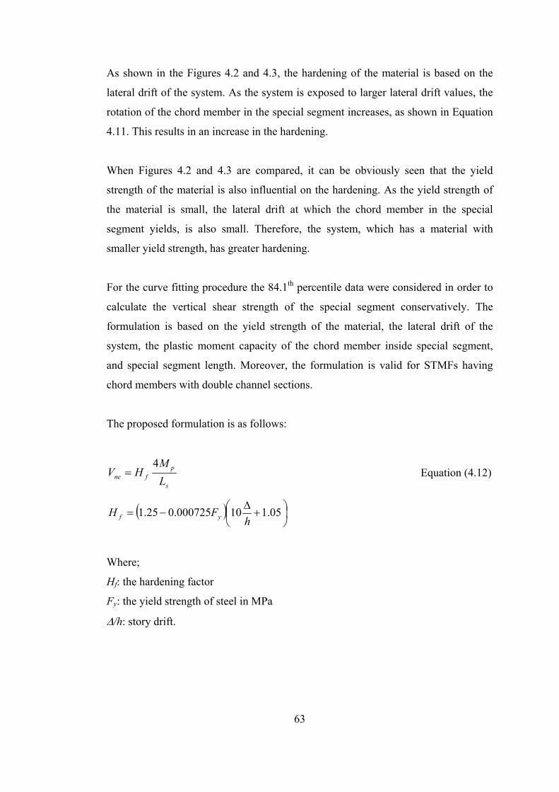
63

As shown in the Figures 4.2 and 4.3, the hardening of the material is based on the

lateral drift of the system. As the system is exposed to larger lateral drift values, the

rotation of the chord member in the special segment increases, as shown in Equation

4.11. This results in an increase in the hardening.

When Figures 4.2 and 4.3 are compared, it can be obviously seen that the yield

strength of the material is also influential on the hardening. As the yield strength of

the material is small, the lateral drift at which the chord member in the special

segment yields, is also small. Therefore, the system, which has a material with

smaller yield strength, has greater hardening.

For the curve fitting procedure the 84.1th percentile data were considered in order to

calculate the vertical shear strength of the special segment conservatively. The

formulation is based on the yield strength of the material, the lateral drift of the

system, the plastic moment capacity of the chord member inside special segment,

and special segment length. Moreover, the formulation is valid for STMFs having

chord members with double channel sections.

The proposed formulation is as follows:

s

pfne L

MHV

4= Equation (4.12)

( ) ⎟⎠⎞

⎜⎝⎛ +

Δ−= 05.110000725.025.1

hFH yf

Where;

Hf: the hardening factor

Fy: the yield strength of steel in MPa

Δ/h: story drift.

64

The formulation in the AISC Seismic Specification (2005) was named as Vne1, the

formulation proposed by Chao and Goel (2008a) was named as Vne2, the proposed

formulation indicated in Equation 4.12 was named as Vne3, and the results obtained

from finite element analysis was named as Vansys in the Tables 4.5 through 4.10.

Since story drift was used as 3% in past formulations, the same value was used in

Equation 4.12 to calculate the expected vertical shear strength of the special segment.

The expected vertical shear strength of the special segment obtained by the

formulations are compared with the analysis results obtained for 3% story drift in the

following tables. The graphical illustrations of these tables are given in Figures 4.4

through 4.9. The statistical quantities including all cases are tabulated in Table 4.11.

65

Table 4.5: Comparison of Results for 2m Ls and A36 Type of Steel

System Vne1 kN Vne2 kN Vne3 kN Vansys kN Vne1/Vansys

(Ratio 1)

Vne2/Vansys

(Ratio 2)

Vne3/Vansys

(Ratio 3)

1 6088.24 4029.08 1609.87 1637.56 3.72 2.46 0.98 2 4707.21 3103.27 1193.89 1176.97 4.00 2.64 1.01 3 2537.91 1708.34 794.36 824.93 3.08 2.07 0.96 4 2246.09 1509.09 690.95 707.94 3.17 2.13 0.98 5 1693.07 1162.46 627.50 658.28 2.57 1.77 0.95 6 1280.87 875.05 455.93 471.14 2.72 1.86 0.97 7 1018.03 703.62 397.18 411.86 2.47 1.71 0.96 8 788.91 542.53 296.12 298.14 2.65 1.82 0.99 9 618.44 431.47 258.52 262.95 2.35 1.64 0.98

10 488.27 346.50 229.14 233.65 2.09 1.48 0.98 11 374.32 264.07 168.98 168.45 2.22 1.57 1.00 12 327.16 236.33 171.33 173.12 1.89 1.37 0.99 13 242.24 173.68 121.27 120.45 2.01 1.44 1.01 14 77.90 58.38 49.82 47.10 1.65 1.24 1.06 15 38.51 29.92 29.14 26.82 1.44 1.12 1.09 16 9881.63 6452.82 2242.07 2169.29 4.56 2.97 1.03 17 8423.61 5489.06 1861.34 1764.27 4.77 3.11 1.06 18 4847.26 3242.21 1428.91 1451.79 3.34 2.23 0.98 19 3855.15 2568.43 1092.83 1070.86 3.60 2.40 1.02 20 4219.91 2842.19 1327.85 1338.99 3.15 2.12 0.99 21 3648.75 2451.17 1121.03 1112.48 3.28 2.20 1.01 22 3127.25 2094.34 933.02 897.56 3.48 2.33 1.04 23 2559.38 1751.43 923.62 923.80 2.77 1.90 1.00 24 2030.53 1383.05 705.05 688.84 2.95 2.01 1.02 25 1637.88 1113.97 561.69 542.31 3.02 2.05 1.04 26 375.87 257.92 138.66 148.16 2.54 1.74 0.94 27 1403.06 965.38 528.79 516.45 2.72 1.87 1.02 28 1087.79 757.55 448.88 439.06 2.48 1.73 1.02 29 929.26 647.61 385.43 382.44 2.43 1.69 1.01 30 396.88 276.29 163.34 166.83 2.38 1.66 0.98 31 841.88 595.18 385.43 376.05 2.24 1.58 1.02 32 549.23 393.78 274.97 262.50 2.09 1.50 1.05 33 483.21 347.03 244.42 234.26 2.06 1.48 1.04 34 202.60 145.06 100.59 99.01 2.05 1.47 1.02 35 68.12 53.17 52.64 48.37 1.41 1.10 1.09

66

Table 4.6: Comparison of Results for 2.5m Ls and A36 Type of Steel


(Ratio 1)

Vne2/Vansys

(Ratio 2)

Vne3/Vansys

(Ratio 3)

1 3256.70 2351.76 1287.90 1301.41 2.50 1.81 0.99 2 2507.41 1803.11 955.11 947.63 2.65 1.90 1.01 3 1383.17 1017.21 635.49 642.87 2.15 1.58 0.99 4 1221.62 896.64 552.76 554.98 2.20 1.62 1.00 5 943.00 707.78 502.00 506.70 1.86 1.40 0.99 6 709.51 529.84 364.75 364.66 1.95 1.45 1.00 7 571.14 431.52 317.74 317.29 1.80 1.36 1.00 8 440.18 330.91 236.90 231.47 1.90 1.43 1.02 9 350.54 267.30 206.82 202.30 1.73 1.32 1.02

10 281.96 218.53 183.31 178.80 1.58 1.22 1.03 11 214.77 165.53 135.18 129.94 1.65 1.27 1.04 12 192.62 151.74 137.06 132.20 1.46 1.15 1.04 13 141.46 110.68 97.02 92.58 1.53 1.20 1.05 14 47.74 38.83 39.86 36.24 1.32 1.07 1.10 15 24.54 20.55 23.31 20.60 1.19 1.00 1.13 16 5208.82 3706.16 1793.65 1781.81 2.92 2.08 1.01 17 4429.90 3144.39 1489.07 1460.08 3.03 2.15 1.02 18 2623.45 1916.41 1143.13 1144.53 2.29 1.67 1.00 19 2077.44 1511.13 874.27 856.19 2.43 1.76 1.02 20 2301.33 1693.47 1062.28 1052.16 2.19 1.61 1.01 21 1984.22 1456.16 896.83 879.54 2.26 1.66 1.02 22 1694.85 1239.72 746.42 718.30 2.36 1.73 1.04 23 1420.32 1062.46 738.90 722.58 1.97 1.47 1.02 24 1121.08 834.64 564.04 542.68 2.07 1.54 1.04 25 902.84 671.14 449.35 429.04 2.10 1.56 1.05 26 209.21 156.94 110.93 112.90 1.85 1.39 0.98 27 783.29 589.16 423.03 404.96 1.93 1.45 1.04 28 615.37 468.41 359.11 341.82 1.80 1.37 1.05 29 526.09 400.74 308.34 296.63 1.77 1.35 1.04 30 224.42 170.77 130.67 128.39 1.75 1.33 1.02 31 484.15 373.89 308.34 291.64 1.66 1.28 1.06 32 320.74 250.96 219.98 204.03 1.57 1.23 1.08 33 282.70 221.54 195.53 181.73 1.56 1.22 1.08 34 118.14 92.32 80.47 76.02 1.55 1.21 1.06 35 43.63 36.67 42.12 37.14 1.17 0.99 1.13

67

Table 4.7: Comparison of Results for 3m Ls and A36 Type of Steel


(Ratio 1)

Vne2/Vansys

(Ratio 2)

Vne3/Vansys

(Ratio 3)

1 2004.10 1565.30 1073.25 1060.02 1.89 1.48 1.01 2 1536.07 1194.99 795.93 778.04 1.97 1.54 1.02 3 868.02 689.48 529.57 519.69 1.67 1.33 1.02 4 765.02 606.58 460.63 449.90 1.70 1.35 1.02 5 604.86 489.23 418.33 407.10 1.49 1.20 1.03 6 452.63 364.49 303.96 294.18 1.54 1.24 1.03 7 368.95 300.13 264.79 255.27 1.45 1.18 1.04 8 282.83 229.08 197.41 187.30 1.51 1.22 1.05 9 228.69 187.50 172.35 162.90 1.40 1.15 1.06

10 187.18 155.54 152.76 143.54 1.30 1.08 1.06 11 141.73 117.24 112.65 104.90 1.35 1.12 1.07 12 130.12 109.56 114.22 106.04 1.23 1.03 1.08 13 94.87 79.44 80.85 74.62 1.27 1.06 1.08 14 33.37 28.80 33.22 29.30 1.14 0.98 1.13 15 17.69 15.59 19.43 16.62 1.06 0.94 1.17 16 3154.73 2429.33 1494.71 1470.48 2.15 1.65 1.02 17 2676.06 2055.91 1240.89 1213.61 2.21 1.69 1.02 18 1634.52 1290.39 952.60 930.35 1.76 1.39 1.02 19 1288.44 1013.20 728.55 701.43 1.84 1.44 1.04 20 1445.15 1148.54 885.23 854.69 1.69 1.34 1.04 21 1242.39 984.96 747.36 716.73 1.73 1.37 1.04 22 1057.47 835.85 622.01 589.41 1.79 1.42 1.06 23 907.76 732.08 615.75 585.53 1.55 1.25 1.05 24 712.86 572.49 470.04 441.88 1.61 1.30 1.06 25 573.15 459.68 374.46 350.27 1.64 1.31 1.07 26 134.11 108.42 92.44 90.15 1.49 1.20 1.03 27 503.57 408.06 352.53 329.19 1.53 1.24 1.07 28 400.71 328.04 299.26 277.19 1.45 1.18 1.08 29 342.83 280.83 256.95 240.05 1.43 1.17 1.07 30 146.08 119.56 108.89 103.42 1.41 1.16 1.05 31 320.18 265.29 256.95 236.03 1.36 1.12 1.09 32 215.10 180.13 183.31 165.47 1.30 1.09 1.11 33 189.90 159.23 162.95 147.10 1.29 1.08 1.11 34 79.12 66.19 67.06 61.27 1.29 1.08 1.09 35 31.58 27.90 35.10 30.03 1.05 0.93 1.17

68

Table 4.8: Comparison of Results for 2m Ls and A572-Gr50 Type of Steel


(Ratio 1)

Vne2/Vansys

(Ratio 2)

Vne3/Vansys

(Ratio 3)

1 6494.56 4419.15 2089.65 2092.32 3.10 2.11 1.00 2 5008.54 3392.55 1549.70 1518.62 3.30 2.23 1.02 3 2738.40 1900.81 1031.10 1060.50 2.58 1.79 0.97 4 2420.48 1676.51 896.87 912.51 2.65 1.84 0.98 5 1851.45 1314.50 814.51 849.43 2.18 1.55 0.96 6 1395.95 985.52 591.81 608.92 2.29 1.62 0.97 7 1118.28 799.85 515.55 533.85 2.09 1.50 0.97 8 863.65 614.28 384.37 386.64 2.23 1.59 0.99 9 683.69 494.11 335.56 341.92 2.00 1.45 0.98

10 546.11 402.02 297.43 304.62 1.79 1.32 0.98 11 416.97 305.02 219.34 219.86 1.90 1.39 1.00 12 370.40 277.84 222.39 226.40 1.64 1.23 0.98 13 272.85 203.06 157.41 157.71 1.73 1.29 1.00 14 90.48 70.45 64.67 62.23 1.45 1.13 1.04 15 45.87 36.98 37.83 35.57 1.29 1.04 1.06 16 10447.51 6996.07 2910.26 2786.88 3.75 2.51 1.04 17 8893.40 5940.06 2416.07 2283.82 3.89 2.60 1.06 18 5207.91 3588.43 1854.76 1859.90 2.80 1.93 1.00 19 4130.98 2833.22 1418.52 1383.25 2.99 2.05 1.03 20 4555.05 3163.92 1723.58 1717.91 2.65 1.84 1.00 21 3931.69 2722.80 1455.13 1433.08 2.74 1.90 1.02 22 3362.74 2320.41 1211.08 1163.59 2.89 1.99 1.04 23 2792.50 1975.22 1198.88 1194.23 2.34 1.65 1.00 24 2208.49 1553.89 915.18 893.31 2.47 1.74 1.02 25 1779.65 1250.06 729.09 705.26 2.52 1.77 1.03 26 410.87 291.52 179.98 191.35 2.15 1.52 0.94 27 1536.52 1093.51 686.38 671.03 2.29 1.63 1.02 28 1201.09 866.32 582.66 571.17 2.10 1.52 1.02 29 1026.54 741.00 500.30 497.43 2.06 1.49 1.01 30 438.10 315.87 212.02 216.92 2.02 1.46 0.98 31 939.16 688.57 500.30 491.04 1.91 1.40 1.02 32 618.63 460.41 356.92 344.26 1.80 1.34 1.04 33 544.90 406.25 317.26 307.21 1.77 1.32 1.03 34 227.99 169.44 130.57 129.62 1.76 1.31 1.01 35 81.41 65.93 68.33 64.06 1.27 1.03 1.07

69

Table 4.9: Comparison of Results for 2.5m Ls and A572-Gr50 Type of Steel


(Ratio 1)

Vne2/Vansys

(Ratio 2)

Vne3/Vansys

(Ratio 3)

1 3581.76 2663.82 1671.72 1676.09 2.14 1.59 1.00 2 2748.48 2034.53 1239.76 1228.61 2.24 1.66 1.01 3 1543.57 1171.19 824.88 835.19 1.85 1.40 0.99 4 1361.14 1030.57 717.50 721.67 1.89 1.43 0.99 5 1069.70 829.41 651.61 660.84 1.62 1.26 0.99 6 801.57 618.22 473.45 476.37 1.68 1.30 0.99 7 651.34 508.51 412.44 415.31 1.57 1.22 0.99 8 499.97 388.31 307.50 303.37 1.65 1.28 1.01 9 402.74 317.41 268.45 265.76 1.52 1.19 1.01

10 328.23 262.94 237.95 235.19 1.40 1.12 1.01 11 248.89 198.28 175.47 171.24 1.45 1.16 1.02 12 227.21 184.95 177.91 174.33 1.30 1.06 1.02 13 165.95 134.19 125.93 122.30 1.36 1.10 1.03 14 57.80 48.49 51.74 48.23 1.20 1.01 1.07 15 30.42 26.20 30.26 27.48 1.11 0.95 1.10 16 5661.53 4140.76 2328.21 2289.34 2.47 1.81 1.02 17 4805.74 3505.19 1932.85 1890.10 2.54 1.85 1.02 18 2911.96 2193.39 1483.81 1481.15 1.97 1.48 1.00 19 2298.10 1722.96 1134.82 1112.56 2.07 1.55 1.02 20 2569.44 1950.86 1378.87 1364.92 1.88 1.43 1.01 21 2210.58 1673.46 1164.11 1143.13 1.93 1.46 1.02 22 1883.24 1420.58 968.87 936.76 2.01 1.52 1.03 23 1606.82 1241.50 959.11 942.75 1.70 1.32 1.02 24 1263.45 971.30 732.14 709.27 1.78 1.37 1.03 25 1016.25 780.02 583.27 561.43 1.81 1.39 1.04 26 237.21 183.81 143.99 147.29 1.61 1.25 0.98 27 890.06 691.66 549.11 530.65 1.68 1.30 1.03 28 706.00 555.43 466.13 449.22 1.57 1.24 1.04 29 603.92 475.45 400.24 389.81 1.55 1.22 1.03 30 257.40 202.43 169.61 168.66 1.53 1.20 1.01 31 561.97 448.60 400.24 384.27 1.46 1.17 1.04 32 376.26 304.26 285.54 269.75 1.39 1.13 1.06 33 332.05 268.92 253.81 240.20 1.38 1.12 1.06 34 138.45 111.82 104.45 100.46 1.38 1.11 1.04 35 54.26 46.88 54.67 49.51 1.10 0.95 1.10

70

Table 4.10: Comparison of Results for 3m Ls and A572-Gr50 Type of Steel


(Ratio 1)

Vne2/Vansys

(Ratio 2)

Vne3/Vansys

(Ratio 3)

1 2274.98 1825.34 1393.10 1378.46 1.65 1.32 1.01 2 1736.96 1387.84 1033.13 1014.64 1.71 1.37 1.02 3 1001.68 817.80 687.40 680.78 1.47 1.20 1.01 4 881.28 718.19 597.92 589.77 1.49 1.22 1.01 5 710.45 590.59 543.01 535.29 1.33 1.10 1.01 6 529.35 438.13 394.54 387.12 1.37 1.13 1.02 7 435.78 364.29 343.70 336.52 1.29 1.08 1.02 8 332.66 276.92 256.25 247.29 1.35 1.12 1.04 9 272.19 229.26 223.71 215.37 1.26 1.06 1.04

10 225.73 192.56 198.29 190.02 1.19 1.01 1.04 11 170.16 144.53 146.22 139.10 1.22 1.04 1.05 12 158.95 137.23 148.26 140.70 1.13 0.98 1.05 13 115.27 99.03 104.94 99.14 1.16 1.00 1.06 14 41.75 36.84 43.12 39.15 1.07 0.94 1.10 15 22.59 20.30 25.22 22.26 1.01 0.91 1.13 16 3531.99 2791.49 1940.18 1902.63 1.86 1.47 1.02 17 2989.25 2356.58 1610.71 1575.76 1.90 1.50 1.02 18 1874.95 1521.20 1236.51 1214.70 1.54 1.25 1.02 19 1472.33 1189.72 945.68 917.88 1.60 1.30 1.03 20 1668.58 1363.04 1149.06 1118.40 1.49 1.22 1.03 21 1431.02 1166.05 970.09 939.18 1.52 1.24 1.03 22 1214.46 986.56 807.39 773.47 1.57 1.28 1.04 23 1063.17 881.27 799.25 769.58 1.38 1.15 1.04 24 831.49 686.38 610.12 582.04 1.43 1.18 1.05 25 667.67 550.41 486.06 461.61 1.45 1.19 1.05 26 157.44 130.82 119.99 118.63 1.33 1.10 1.01 27 592.55 493.48 457.59 434.58 1.36 1.14 1.05 28 476.24 400.55 388.44 366.77 1.30 1.09 1.06 29 407.69 343.09 333.53 317.54 1.28 1.08 1.05 30 173.57 145.94 141.34 136.74 1.27 1.07 1.03 31 385.03 327.55 333.53 312.78 1.23 1.05 1.07 32 261.36 224.54 237.95 220.00 1.19 1.02 1.08 33 231.03 198.71 211.51 195.51 1.18 1.02 1.08 34 96.05 82.44 87.04 81.42 1.18 1.01 1.07 35 40.44 36.41 45.56 40.20 1.01 0.91 1.13

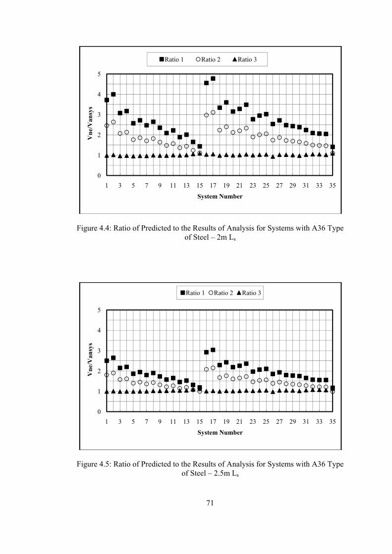
71

Figure 4.4: Ratio of Predicted to the Results of Analysis for Systems with A36 Type of Steel – 2m Ls

Figure 4.5: Ratio of Predicted to the Results of Analysis for Systems with A36 Type of Steel – 2.5m Ls

0

1

2

3

4

5

1 3 5 7 9 11 13 15 17 19 21 23 25 27 29 31 33 35

Vne

/Van

sys

System Number

Ratio 1 Ratio 2 Ratio 3

0

1

2

3

4

5

1 3 5 7 9 11 13 15 17 19 21 23 25 27 29 31 33 35

Vne

/Van

sys

System Number


72

Figure 4.6: Ratio of Predicted to the Results of Analysis for Systems with A36 Type of Steel – 3m Ls

Figure 4.7: Ratio of Predicted to the Results of Analysis for Systems with A572-Gr50 Type of Steel – 2m Ls

0

1

2

3

4

5

1 3 5 7 9 11 13 15 17 19 21 23 25 27 29 31 33 35

Vne

/Van

sys

System Number


0

1

2

3

4

5

1 3 5 7 9 11 13 15 17 19 21 23 25 27 29 31 33 35

Vne

/Van

sys

System Number


73

Figure 4.8: Ratio of Predicted to the Results of Analysis for Systems with A572-Gr50 Type of Steel – 2.5m Ls

Figure 4.9: Ratio of Predicted to the Results of Analysis for Systems with A572-Gr50 Type of Steel – 3m Ls

0

1

2

3

4

5

1 3 5 7 9 11 13 15 17 19 21 23 25 27 29 31 33 35

Vne

/Van

sys

System Number


0

1

2

3

4

5

1 3 5 7 9 11 13 15 17 19 21 23 25 27 29 31 33 35

Vne

/Van

sys

System Number


74

Table 4.11: Statistical Values for All Cases Statistical Quantity Vne1/Vansys Vne2/Vansys Vne3/Vansys

Maximum 4.77 3.11 1.17 Minimum 1.01 0.91 0.94 Average 1.92 1.44 1.03

Standard Deviation 0.68 0.39 0.04

The formulation in the AISC Seismic Specification (2005) significantly

overestimated the results. However, the updated version of this formulation, which

was proposed by Chao and Goel (2008a), estimated the results better, as can be

observed from the Tables 4.5 through 4.10. As the length of the special segment

increases and the moment of inertia of the chord section decreases, the result of the

formulation proposed by Chao and Goel (2008a) is closer to the result of the finite

element analysis. As the length of the special segment increases and the moment of

inertia of the section decreases, the stiffness of the chord member in the special

segment decreases. Therefore, the stiffness of the chord member in the special

segment is significantly lower than the stiffness of the neighboring chord members.

As a result of this, the end conditions of the chord member in the special segment

approaches to the fixed-end case and the elastic stiffness assumption of Chao and

Goel (2008a), as discussed in the first section, is appropriate. However, for smaller

lengths of the special segment and chord sections with higher moment of inertia, the

proposed formulation by Chao and Goel (2008a) significantly overestimated the

results.

The proposed formulation in this chapter, Equation 4.12, showed a good agreement

with the analysis results, as shown from the Figure 4.4 through 4.9. This proposed

formulation is only 6 percent unconservative, as shown from the Table 4.11. This

value is tolerable for design purposes. Moreover, the accuracy of the proposed

formulation is the best when compared with the other formulations, as indicated in

Table 4.11.

75

CHAPTER 5

5AN EVALUATION OF SHEAR CONTRIBUTION BY X-DIAGONALS FOR STMF SYSTEMS

The special segments in STMF systems can include X-braces. The design of the

special segments with X-bracing is similar to the design of vierendeel segments.

First of all, the required shear strength of the special segment is determined by

considering all possible load combinations. The AISC Seismic Specification (2005)

mandates that the shear resistance of the X-diagonals be limited to 75 percent of the

total shear resistance. In other words, at least 25 percent of the shear force should be

resisted by the chord members.

Unlike the provisions for braced frames there are no specific brace slenderness

requirements for the X-braces in STMF systems. In fact the use of flat bars as X-

bracing is recommended in the AISC Seismic Specification (2005). Therefore,

engineers can choose very slender members that have low energy dissipating

capacity.

In this chapter, the shear contribution of the X-diagonals to the total required shear

strength, named as the load share, as well as the influence of brace slenderness are

evaluated from a performance-based point of view.

5.1 Methodology and Design of the Systems

To be able to compare X-diagonals with different load shares, five different systems

were considered. The load shares of these systems were 10%, 25%, 50%, 75%, and

90%. Moreover, for each load share of the X-diagonals, the diagonal elements in the

special segment were designed by using two extreme values of slenderness, which

76

were zero and infinity. For the systems having X-diagonals with zero slenderness,

the diagonals can develop their yield strength capacity under compression. For the

systems having X-diagonals with infinite slenderness, the diagonals have no

compression strength. The extreme slenderness values were considered to study the

effects of the slenderness of the X-diagonals on the performance of the whole

system.

The model studied is a one story frame, which has a span length of 10m, a panel

length of 1m, a special segment consisted of two panels and a height of 3.5m, as

shown in Figure 5.1.

Figure 5.1: Geometrical Properties of the Systems

The member sections outside the special segment were the same in order not to

introduce any other parameters to the study. All the members outside the special

segment were modeled with elastic elements, as given in Table 5.1.

The members inside the special segment, namely the chord members and the X-

diagonals, were selected by considering the load share and the slenderness of the X-

diagonals. The shear strength of the special segment was taken as 360 kN and kept

10m

2m

1m

2.5m

Special Segment

77

constant for each case to be able to make a fair comparison between the different

systems. The cross-section types, material properties, and element types for each

case are given in Table 5.2.

Table 5.1: The Members outside the Special Segment

A bilinear kinematic hardening with 1 percent of the initial elastic modulus of the

material, as verified in Chapter 2, was used for the modeling material behavior of the

chords. However, for the material of the diagonals of the special segment, elastic

perfectly plastic material was used. The diagonals with zero slenderness were

modeled with ordinary two node truss elements. For diagonals with infinite

slenderness, tension-only truss elements were utilized. It should be mentioned that

certain amount of inaccuracy is introduced by modeling the braces as tension-only

elements. Basically, from a strength point of view these elements are capable of

representing the loss of strength under compressive forces. However, from a stiffness

point of view the loss of stiffness due to buckling is not adequately addressed. In

earlier stages of research, the braces were modeled with beam-column elements as

recommended by Uriz, Fillipou, and Mahin (2008). The recommended formulation

failed to capture the response of the braces under earthquake excitation. Therefore,

an alternative modeling technique was adopted in this study.

Load Share %

Slenderness of X-Diagonals

inside the S.S. Element Section Element Model

For All Load

Shares

For All Slenderness

Values

Columns W14x370 Elastic Beam-Column Chords outside

the S.S. 2MC12x35 Elastic Beam-Column

Diagonals outside the S.S. 2L5x5x5/16 Truss

Verticals 2L3x3x1/2 Truss

78

Table 5.2: The Members inside the Special Segment

Load Share

%


inside the S.S. Element Section Zx mm3 A mm2 Element

Model Fy

MPa

10

Zero

Chords inside the

S.S. 2C10x15.3 5.21x105 2890.32

Nonlinear Beam-

Column 310

Diagonals inside the

S.S - - 72.73 Truss 310

Infinity

Chords inside the

S.S. 2C10x15.3 5.21x105 2890.32

Nonlinear Beam-

Column 310


S.S - - 145.46 Truss 310

25

Zero

Chords inside the

S.S. 2C9x13.4 4.13x105 5083.86

Nonlinear Beam-

Column 335


S.S - - 181.83 Truss 335

Infinity

Chords inside the

S.S. 2C9x13.4 4.13x105 5083.86

Nonlinear Beam-

Column 335


S.S - - 363.66 Truss 335

50

Zero

Chords inside the

S.S. 2C7x12.2 2.77x105 4645.15

Nonlinear Beam-

Column 350


S.S - - 363.66 Truss 350

Infinity

Chords inside the

S.S. 2C7x12.2 2.77x105 4645.15

Nonlinear Beam-

Column 350


S.S - - 727.32 Truss 350

75

Zero

Chords inside the

S.S. 2C5x9 1.44x105 3406.45

Nonlinear Beam-

Column 360


S.S - - 545.48 Truss 360

Infinity

Chords inside the

S.S. 2C5x9 1.44x105 3406.45

Nonlinear Beam-

Column 360


S.S - - 1090.96 Truss 360

79

Table 5.2 (continued)

5.2 Static Pushover Analysis and Natural Periods

A set of pushover analysis was conducted to verify the designs in terms of a strength

point of view. The idea was to prove that the systems selected essentially provide the

same amount of lateral strength at a lateral drift of 3%. The pushover characteristic

of the systems having the X-diagonal members inside the special segment with zero

slenderness and infinite slenderness are given in Figure 5.2 and Figure 5.3,

respectively.

As shown from the Figures 5.2 and 5.3, the capacities of the models are close to each

other and reach to 1100 kN at 3 percent lateral drift. Moreover, as the load share of

X-diagonals increase, the stiffness of the system also increases. This is natural

because as the load share increases, the behavior shifts from a moment frame

behavior to a braced frame behavior.

Load Share

%


inside the S.S. Element Section Zx mm3 A mm2 Element

Model Fy

MPa

90

Zero

Chords inside the

S.S. 2C3x6 0.57x105 2270.96

Nonlinear Beam-

Column 370


S.S - - 654.58 Truss 370

Infinity

Chords inside the

S.S. 2C3x6 0.57x105 2270.96

Nonlinear Beam-

Column 370


S.S - - 1309.16 Truss 370

80

Figure 5.2: Pushover Analysis Results for Systems Having X-Diagonals with Zero

Slenderness

Figure 5.3: Pushover Analysis Results for Systems Having X-Diagonals with Infinite

Slenderness

0100200300400500600700800900

100011001200

0 0.5 1 1.5 2 2.5 3 3.5

Bas

e Sh

ear,

kN

Lateral Drift, %

10% 25% 50% 75% 90%

0100200300400500600700800900

100011001200

0 0.5 1 1.5 2 2.5 3 3.5

Bas

e Sh

ear,

kN

Lateral Drift, %

10% 25% 50% 75% 90%

81

The responses of the systems for cyclic pushover analysis are needed to evaluate the

effect of different slenderness values on the strength of the systems. The results of

the cyclic pushover analysis are given in Figure 5.4 and Figure 5.5, for the systems

having X-diagonals with zero slenderness and with infinite slenderness, respectively.

For systems having X-diagonals with zero slenderness, there is no degradation in the

strength and stiffness, as shown in Figure 5.4. However, for systems having X-

diagonals with infinite slenderness, the pinching of system takes place, as shown in

Figure 5.5. The degree of pinching significantly increases, when the load share of X-

diagonals increases, as expected, since the X-diagonal members in the special

segment do not carry compressive forces.

Apart from pushover analysis, an eigenvalue analysis was conducted for each STMF

to obtain the natural period of the systems. The natural period and the mass

properties of the systems are given in Table 5.3.


Zero Slenderness

-1500

-1000

-500

0

500

1000

1500

-4 -3 -2 -1 0 1 2 3 4

Bas

e Sh

ear,

kN

Lateral Drift, %

10% 25% 50% 75% 90%

82

Figure 5.5: Cyclic Pushover Analysis Results for Systems Having X-Diagonals with Infinite Slenderness

Table 5.3: Natural Period and Mass of the STMF Systems

Load Share % Slenderness of X-Diagonals inside the S.S. Mass ton T sec

10 Zero 125 0.376

Infinity 125 0.363

25 Zero 125 0.360

Infinity 125 0.344

50 Zero 125 0.346

Infinity 125 0.333

75 Zero 125 0.339

Infinity 125 0.328

90 Zero 125 0.336

Infinity 125 0.327

-1500

-1000

-500

0

500

1000

1500

-4 -3 -2 -1 0 1 2 3 4

Bas

e Sh

ear,

kN

Lateral Drift, %

10% 25% 50% 75% 90%

83

As shown in Table 5.3, as the load share of the X-diagonals increases, the natural

period decreases, in other words, the stiffness of the system increases. For a

particular load share, the natural period of the system having X-diagonals with

infinite slenderness is slightly lower than the natural period of the system having X-

diagonals with zero slenderness, as shown in Table 5.3. This is because the area of

X-diagonals with infinite slenderness needs to be twice the area of its counterpart to

keep the same level of strength. Therefore, the stiffness of the systems having X-

diagonals with infinite slenderness is greater than the other one, in other words, these

systems have a lower natural periods than the others. However, in a general sense,

the natural periods of the systems are close to each other.

5.3 Time-History Analysis

A set of time-history analysis were conducted to study the behavior of systems under

earthquake loading. All structures were subjected to a suite of ground motions listed

in Table 3.4, except the twentieth ground motion. The twentieth ground motion was

excluded from the set because it produced numerical instabilities in the solution

process. A stiffness proportional damping equal to 2 percent of the critical damping

was considered in all analysis.

During a typical analysis, story drift, curvatures at the chords of the special segment,

the base shear, and the axial strain at the X-diagonals were recorded.

5.3.1 Results of Time-History Analysis

In order to compare the performance of the systems, the average values of the

recorded maximum responses obtained from the analysis of nineteen different

ground motions were considered. In Table 5.4, the average values of the results of

time-history analysis are tabulated. In this table, curvature at the chords of the special

segment and axial strain at the X-diagonals are normalized with the plastic curvature

and yield axial strain, respectively. These normalizations were used for expressing

the curvatures and the axial strains in terms of demands and provided a fair

84

comparison tool between different designs. Moreover, the graphical illustrations of

the time-history analysis results are given in Figures 5.6 through 5.9.

Table 5.4: The Average Values of the Results of Time History Analysis

Figure 5.6: Average Normalized Curvature Values for Different Design Types

0

5

10

15

20

25

30

35

40

45

0 20 40 60 80 100

Ave

rage

Nor

mal

ized

Cur

vatu

re

Load Share of X-Diagonals, %

Zero Slenderness Infinite Slenderness

Load Share 10% 25% 50% 75% 90%

Slenderness 0 ∞ 0 ∞ 0 ∞ 0 ∞ 0 ∞

(k/kp)average 40.5 36.6 30.0 31.0 18.8 20.7 10.9 13.6 4.5 7.1

(ε/εy)average 19.3 18.0 16.2 16.5 13.8 14.6 11.9 13.5 10.5 13.1

(Vb)average kN 931 931 939 946 969 988 981 1035 1007 1042

(Δ/h)average % 1.40 1.34 1.32 1.34 1.25 1.30 1.17 1.27 1.12 1.28

85

Figure 5.7: Average Normalized Axial Strain Values for Different Design Types

Figure 5.8: Average Base Shear Values for Different Design Types

0

4

8

12

16

20

0 20 40 60 80 100

Ave

rage

Nor

mal

ized

A

xial

Str

ain



0

150

300

450

600

750

900

1050

1200

0 20 40 60 80 100

Ave

rage

Bas

e Sh

ear,

kN



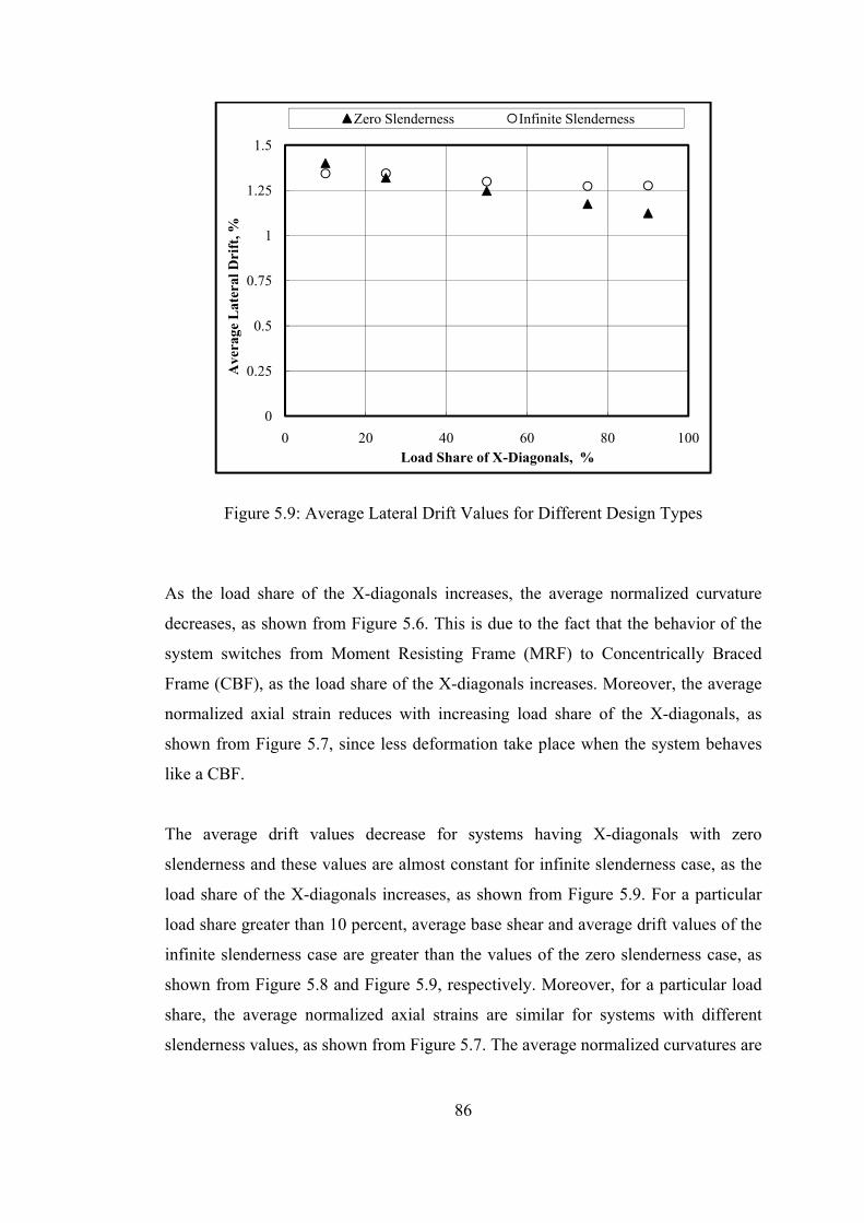
86

Figure 5.9: Average Lateral Drift Values for Different Design Types

As the load share of the X-diagonals increases, the average normalized curvature

decreases, as shown from Figure 5.6. This is due to the fact that the behavior of the

system switches from Moment Resisting Frame (MRF) to Concentrically Braced

Frame (CBF), as the load share of the X-diagonals increases. Moreover, the average

normalized axial strain reduces with increasing load share of the X-diagonals, as

shown from Figure 5.7, since less deformation take place when the system behaves

like a CBF.

The average drift values decrease for systems having X-diagonals with zero

slenderness and these values are almost constant for infinite slenderness case, as the

load share of the X-diagonals increases, as shown from Figure 5.9. For a particular

load share greater than 10 percent, average base shear and average drift values of the

infinite slenderness case are greater than the values of the zero slenderness case, as

shown from Figure 5.8 and Figure 5.9, respectively. Moreover, for a particular load

share, the average normalized axial strains are similar for systems with different

slenderness values, as shown from Figure 5.7. The average normalized curvatures are

0

0.25

0.5

0.75

1

1.25

1.5

0 20 40 60 80 100

Ave

rage

Lat

eral

Dri

ft, %



87

similar for systems with different slenderness values for a particular load distribution

up to 90 percent load share, as shown from Figure 5.6.

To conclude, the amount of the load share of the X-diagonals has a significant effect

on the behavior of the system. If this amount increases then the system behavior

switches from MRF to CBF. However, although two theoretically extreme

slenderness values were used, the slenderness value of the X-diagonals does not have

any significant effects on the seismic performance of the system.

88

CHAPTER 6

6CONCLUSIONS

The thesis work consisted of a three phase of numerical study on STMF systems. The

numerical analyses of phase 1 and 3 was conducted using OPENSEES, while 3-D

finite element analyses of phase 2 was performed using ANSYS.

For the first phase of the study, the seismic behavior of STMF system with a

vierendeel special segment designed using three different methodologies was

explored. Six, nine, and twelve story frames were designed using plastic and elastic

design methods. Elastic design of frames was conducted using IT (inverted

triangular) and CGL (proposed by Chao, Goel, and Lee (2008b)) lateral load

distributions. The results of static pushover analysis and time-history analysis were

utilized in order to compare the strength and the seismic performance of the systems.

For the second phase of the study, the expected vertical shear strength formulations

were evaluated using three dimensional finite element analysis results. A single story

STMF system with vierendeel special segment was considered. The parameters were

the chord section in the special segment and the length of the special segment. For

thirty five double channel sections and three different lengths of special segment,

pushover analyses up to 3 percent lateral drift were conducted. The earlier

formulations and the formulation developed in this phase, Equation 4.12, were

compared with the finite element analysis results.

For the third phase of the study, single story STMF systems with X-diagonal special

segment were evaluated in terms of the shear contribution and the slenderness of the

89

X-diagonals. To accomplish this, the frames were designed considering five different

load shares of X-diagonals. For each load share, X-diagonals were designed with

zero and infinite slenderness values. In order to compare the strength and the seismic

performance of the frames, static pushover and time-history analyses were

conducted.

The following can be concluded from the first phase of the study:

• For all types of design and all heights, the maximum base shear and

maximum top story drift relation obtained from time-history analysis results

can be best predicted using the static pushover analysis with the equal lateral

load distribution.

• For ED-IT and ED-CGL, there were no significant changes in plastic

rotations and story drifts. The ED-CGL improved the behavior at some levels

and deteriorated in others. Since the use of the ED-CGL is based on

predicting the natural period of the system before the design is finalized, the

ED-IT is more useful.

• Utilizing PD increased the lateral drifts at bottom stories, however, decreased

the lateral drifts at the top stories. While the use of PD increased the plastic

rotations at bottom stories, significantly reduced them at the top stories. As

long as the increases in the lateral drift and in the plastic rotation at bottom

stories are tolerable, using PD is a viable option.

The following can be concluded from the second phase of the study:

• The elastic stiffness of the chord member in the special segment assumption

proposed by Chao and Goel (2008a) was not appropriate for all lengths of

special segment and chord sections.

• The expected vertical shear strength of the special segment formulation in the

AISC Seismic Specification (2005) was found to be overly conservative.

• The expected vertical shear strength formulation developed by Chao and

Goel (2008a) is better than the AISC formulation, however, overestimated the

90

results of the finite element analysis for smaller special segment lengths and

chord sections with higher moment of inertia.

• The proposed formulation in this phase of the study, Equation 4.12, was

derived for STMFs having double channel chord members. This formulation

showed a good agreement with the analysis results and was only 6 percent

unconservative.

The following can be concluded from the third phase of the study:

• As the load share of the X-diagonals increased, the average drift values

decreased for systems having X-diagonals with zero slenderness and these

values were almost constant for infinite slenderness case. Moreover, with

increasing load share of the X-diagonals, average base shear values increased

and average normalized curvature and axial strain values decreased.

• As the load share of X-diagonals increased, the behavior of the system

switched from MRF to CBF. Therefore, fewer deformations took place.

• The slenderness of the X-diagonals in the special segment did not have any

significant effects on the seismic response of the system.

Future Research Needs

• The final steel weight of the STMF systems with a vierendeel opening

designed using ED-IT and PD can be compared for economical point of view.

• The expected vertical shear strength at vierendeel opening formulation can be

examined for multistory STMFs and more experimental research is needed to

further verify the accuracy of it.

• The effects of the slenderness and the load share of the X-diagonals on the

behavior of multistory systems can be evaluated.

• The existing and newly developed provisions for STMFs can take place in

Eurocodes.

91

REFERENCES

AISC, 2005. Seismic Provisions for Structural Steel Buildings, ANSI/AISC 341-05, American Institute of Steel Construction, Chicago, Ill. ANSYS. Version 8.1 on-line user’s manual; 2006. Aslani, H.O. (1998). Special truss moment frames under combined gravity and lateral loads. Dissertation, The University of Michigan, Ann Arbor, MI. Basha, H.S., and Goel, S.C. (1994). Seismic resistant truss moment frames with ductile vierendeel segment. Report No. UMCEE 94-29, Department of Civil and Environmental Engineering, The University of Michigan, Ann Arbor, MI. Chao, S., and Goel, S.C. (2006). Performance based plastic design of special truss moment frames. Report No. UMCEE 06-03, Department of Civil and Environmental Engineering, The University of Michigan, Ann Arbor, MI. Chao, S., and Goel, S.C. (2008a). A modified equation for expected maximum shear strength of the special segment for design of special truss moment frames. Engineering Journal; 45(2): 117-125. Chao, S., and Goel, S.C. (2008b). Performance-based plastic design of special truss moment frames. Engineering Journal; 45(2): 127-150. Chao, S., Goel, S.C., and Lee, S.S. (2007). A seismic design lateral force distribution based on inelastic state of structures. Earthquake Spectra; 23(3): 547-569. Goel, S.C., and Itani, A.M. (1994a). Seismic behavior of open-web truss-moment frames. Journal of Structural Engineering; 120(6): 1763-1780. Goel, S.C., and Itani, A.M. (1994b). Seismic-resistant special truss-moment frames. Journal of Structural Engineering; 120(6): 1781-1797. Goel S.C., Leelataviwat S., and Stojadinovic B. (1997). Steel moment frames with ductile girder web openings. AISC Engineering Journal; Fourth Quarter: 115-125. Goel, S.C., Rai, D.C., and Basha, H.S. (1998). Special truss moment frames design guide. Report No. UMCEE 98-44, Department of Civil and Environmental Engineering, The University of Michigan, Ann Arbor, MI.

92

Ireland, R.C. (1997). Special truss moment frames in low to moderate seismic regions with wind. Dissertation, The University of Michigan, Ann Arbor, MI. OPENSEES. Version 2.0 user command-language manual; 2009. Parra-Montesinos, G.J., Goel, S.C., and Kim, K.Y. (2006). Behavior of steel double-channel built-up chords of special truss moment frames under reversed cyclic loading. Journal of Structural Engineering; 132(9): 1343-1351. Uriz, P., Filippou, F.C., and Mahin, S.A. (2008). Model for cyclic inelastic buckling of steel braces. Journal of Structural Engineering; 134(4): 619-628.

a numerical study on special truss moment frames a … · araştırılmıştır. sonlu eleman...

Documents