a numerical study of the equilibrium and nonequillbrlum ...manzanar/pubs/manzanares_pub022.pdf ·...

J. Phys. Chem. 1992, 96, 9983-9991 9983

(17) Yates, J. T.. Jr.; Duncan, T. M.; Worley, S. D.; Vaughan, R. W. J.

(18) Yates, J. T., Jr.; Duncan, T. M.; Vaughan, R. W. J. Chem. Phys.

(19) Solymosi, F.; Sirkiny, J. J . Appl. Surf. Sci. 1979, 3, 68. (20) Sotymosi, F.; Erdahelyi, A.; Kwis, M. J. Coral. 1980, 65, 428. (21) Antonicwicz, P. R.; Cavanagh, R. R.; Yaks, J. T., Jr. J. Chem. Phys.

(22) Cavanagh, R. R.; Yates, J. T., Jr. J . Chem. Phys. 1981, 74, 4150. (23) Rice, C. A,; Worley, S. D.; Curtis, C. W.; Guin, J. A.; Tarrer, A. R.

(24) Yatcs, J. T., Jr.; Cavanagh, R. R. J . C o r d 1982, 74,97. (25) Yates, J. T., Jr.; Kolasinski, K. J. Chem. Phys. 1983, 79, 1026. (26) Robbins, J. L. J. Phys. Chem. 1986.90, 3381. (27) Duncan, T. M.; Root, T. W. J. Phys. Chem. 1988,92, 4426. (28) Thayer, A. M.; Duncan, T. M. J. Phys. Chem. 1989,93,6763. (29) van’t Blik, H. F. J.; van Zon, J. 9. A. D.; Huizinga, T.; Vis, J. C.;

Koningsberger, D. C.; Prins, R. J. Phys. Chem. 1983,87, 2264. (30) van’t Blik, H. F. J.; van Zon, J. B. A. D.; Huizinga, T.; Vis, J. C.;

Koningsberger, D. C.; Prins, R. J. Am. Chem. Soc. 1985, 107, 3139. (31) Solymmi, F.; Pasztor, M. J. Phys. Chem. 1985,89,4789. (32) Solymosi, F.; Pasztor, M. J. Phys. Chem. 1986, 90, 5312.

Chem. Phys. 1979, 70, 1219.

1979, 71, 3908.

1980, 73, 3456.

J. Chem. Phys. 1981, 74, 6487.

(33) Ballinger, T. H.; Yates, J. T., Jr. J . Phys. Chcm. 1991, 95, 1694. (34) Basu, P.; Panayotov, D.; Yates, J. T., Jr. J . Phys. Chem. 1987, 91,

(35) Basu, P.; Panayotov, D.; Yates, J. T., Jr. J. Am. Chem. Soc. 1988, 3133.

110. 2074. (36) Zaki, M. I.; Kunzmann, G.; Gates, B. C.; KnBzinger, H. J . Phys.

(37) Paul, D. K.; Ballinger, T. H.; Yates, J. T., Jr. J. Phys. Chem. 1990, Chem. 1987, 91, 1486.

94, 4617. (38) Zaki, M. I.; Ballinger, T. H.; Yates, J. T., Jr. J . Phys. Chem. 1991,

(39) Ballinger, T. H.; Yates, J. T., Jr. J . Am. Chem. Soc., accepted for

(40) Basu, P.; Ballinger, T. H.; Yates, J. T., Jr. Reo. Sei. Insrrum. 1988,

95, 4028.

publication.

59. 1321. (41) Muha, R. J.; Gates, S. M.; Yates, J. T., Jr.; Basu, P. Rev. Sei.

(42) Hanley, L.; Guo, X.; Yates, J. T., Jr. J . Chem. Phys. 1989,91,7220. (43) Miller, F. A.; Golob, H. R. Spectrochim. Acto 1964, 20, 1517. (44) Muettertia, E. L. Chem. Soc. Rev. 1983,12, 283. (45) Crabtree, R. H. Chem. Rev. 1985,85, 245. (46) Halpern, J. Inorg. Chim. Acro 1985, 100, 41.

Instrum. 1985, 56, 613.

A Numerical Study of the Equilibrium and Nonequillbrlum Diffuse Double Layer in Electrochemical Cells

W. D. Murphy? J. A. Manzanares,t** S. Maf6,t.s and H. Reiw*** Science Center Division, Rockwell International, Thousand Oaks, California 91 360, and Department of Chemistry. University of California, Los Angeles. California 90024 (Received: July 6, 1992; In Final Form: September 1. 1992)

A numerical solution of the Nernst-Planck and Poisson equations is presented. The equations are discretized in a finite difference scheme using the method of l ies on variable spatial and temporal grids. A Gear’s stiffly stable p red ic tmec to r integration procedure which automatically adjusts the order of the predictor and corrector equations (and the step size) to ensure the accuracy of the results is incorporated. Some advantages of our approach over more classical ones are discussed. The numerical solution is applied to the study of the equilibrium and nonequilibrium diffuse electrical double layer (EDL) at the metal electrode/electrolyte solution interface. The prescription of this layer is similar to that used in the classical Gouy-Chapman theory. Electrode kinetics are described by the Butler-Volmer equation. Concentration, faradaic and displacement electric current densities, and electric potential profdea as functions of time a- the cell thickness, and partiahly in the EDL regions at the metal electrode/solution interfaces, are obtained. Two physical problems are studied: (i) the formation of the equilibrium EDL, and (ii) the transient response of the system to an electrical perturbation. Thew examplea illustrate the potential applications of the numerical method.

Numerical techniques for the solution of transport problems in electrochemistry have contributed significantly to the analysis of many complex processes which are difficult to deal with using more conventional approaches. Though other techniques like the boundary element method are experiencing an increasing popu- larity,’ fmite differences2J has been one of the most widely used in electrochemistry since the pioneering work by Feldberg!.s The need for numerical solutions appears in a multitude of problems of practical interest, e.g., transport phenomena described by diffusional type or second-order parabolic PDEs (partial differential equations) subjected to temporal boundary conditions,*J diffusion-migration situations involving the coupled, nonlinear Nemst-Planck and Poisson equations,b10 convective diffusion problems in electrochemical ce l l~ ,~J etc. Modern numerical solutions to the Nemst-Planck and Poisson

equations in electrochemical cells including electrical double layer (EDL) effects seem to be lacking.’ We present, here, a numerical solution of these equations for a system consisting of three ions

To whom correspondence should be addressed. Rockwell International.

‘Permanent add=: Department of Thermodynamics, University of Va- lencia, 46100 Burjasot, Spain.

8 University of California.

having different charges and undergoing transport in an electrochemical cell. Transport is assumed to occur in one dimension. Special attention is paid to the evolution of the diffuse EDL. This layer is considered to consist of point ions in a continuous dielectric solvent with local potential of mean force taken to be the electrical potential, i.e., the system is prescribed in a manner similar to that employed in the classical Gouy-Chapman theory.’* Electrode kinetia are described by a Butler-Volmer-type equation that takes into account the structure of the nonequilibrium EDL.12 The numerical solution gives concentration, faradaic and displacement electric currents, the electric potential profiles as functions of time across the cell thickness, and, particularly in the EDL regions, at the metal electrode/solution interfaces.

The numerical technique used is of the finite difference type, and incorporates the Gear’s stiffly stable predictorcorrector method. The equations are discretized using the method of lines on a variable spatial grid because large gradients are present in the EDL region. The time grid is automatically generated by the procedure in order to satisfy a prescribed error tolerance. These characteristia result in a stable and accurate numerical integration of the Nernst-Planck and Poisson equations.

We have considered two problems of well-known complexity: (1) the formation of the equilibrium EDL at the electrode/solution interface, and (2) the electrical relaxation that occurs when an exponentially-shaped external potential perturbation is applied

0022-3654/92/2096-9983$03.00/0 Q 1992 American Chemical Society

9984 The Journul of Physical Chemistry, Vol. 96, No. 24, 1992 Murphy et al.

to the system. These examples illustrate two possible applications of the numerical solution, namely the study of steady state and equilibrium problems, and the analysis of the tramient responre to an electrical perturbation. To further test the procedure, we have derived solutions for the steady-state equations in some simplified cases and compared them to the exact numerical solutions.

The system of Nernst-Planck and Poisson equations is mul- tidisciplinary, in the sense that it appears in many fields of science and technology where charge transport occurs. Thus, some of the ideas and results discussed here find application in semicon- d u c t o r ~ , ~ ~ synthetic and biological charged membranes,14 and colloids.

Formulation of the Problem As indicated earlier we will focus on a particular problem

involving the Nemst-Planck and Poisson equations. In this problem we deal with the following three one-dimensional Nernst-Planck equations

and the three continuity equations aJi aci

i = 1 , 2 , 3 - =-- ax at'

as well as the Poisson equation

(3)

where Ji, Di, ci, zi denote flux, diffusion coefficient, concentration, and charge number (zl = 2, z2 = -1, z3 = 3) of the ith species, respectively, while x and t stand for the position coordinate and the time, and e for the dielectric permittivity. $ is the electric potential, R the gas constant, T the absolute temperature, and F the Faraday constant. Equation 1 is a simplified form of the flux equation applicable to dilute solutions and derivable by use of the principle of detailed balance. It may also be derived in a somewhat more systematic manner by means of the thermodynamics of irreversible processes. Its origin and limitations can be found elsewhere.I6 For the purposes of the numerical solution it is convenient to express the above equations in dimensionless form. This can be accomplished with the following transformations

[ = x/X (4)

r tD/X2 ( 5 )

u = c,/c, v = c2/c, w = c3/c (6) 4 = $F/RT (7)

where all of the Di have been assumed to be q u a l and repre- sentable by D and c and X are suitable scaling factors having the dimensions of 0o"tratiOn and length, respectively. In particular, X = (cRT/Pc)'/~ is the Debye length characteristic of the electrolyte solution.16 We also introduce a faradaic electric current density H (in dimensionless form) by the definition

n = (W, - 52 + 353)X/DC (8)

Substitution of eqs 4-8 into eqs 1-3 gives

$4 - = -2u + v - 3w = - p at2

(9 )

electrode solution electrode + 3

- e

+ 2

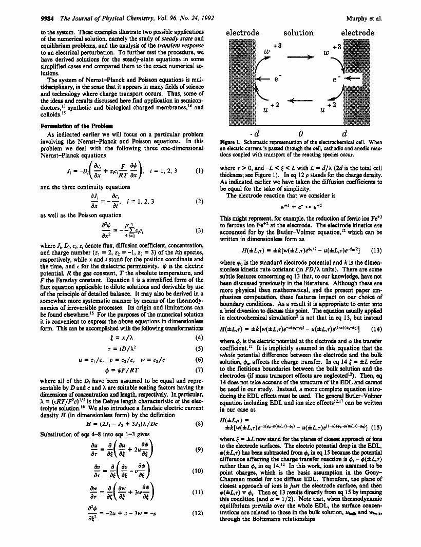
- d 0 d Figure 1. Schematic representation of the electrochemical cell. When an electric current is passed through the cell, cathodic and anodic reactions coupled with transport of the reacting species occur.

where 7 > 0, and -L < C L with L = d/X (2d is the total cell thickness; see Figure 1). In eq 12 p stands for the charge density. As indicated earlier we have taken the diffusion coefficients to be equal for the sake of simplicity.

The electrode reaction that we consider is w+3 + e- +w u+2

This might represent, for example, the reduction of ferric ion Fe+3 to ferrous ion Fe+2 at the electrode. The electrode kinetics are accounted for by the Butler-Volmer equation,12 which can be written in dimensionless form as

H(fL,7) = fk[w(fL,~)&/~ - u(fL,~)e-h/~] (13)

where & is the standard electrode potential and k is the dimensionless kinetic rate constant (in FD/X units). There are some subtle features concerning eq 13 that, to our knowledge, have not been discussed previously in the literature. Although these are more physical than mathematical, and the present paper em- phasizes computation, these features impact on our choice of boundary conditions. As a result it is appropriate to enter into a brief diversion to 4i9cuss this point. The equation usually applied in electrochemical simulation2 is not that in eq 13, but instead

H(fL,7) = fk[w(fL,.r)e-a(4**) - u(fL,~)e('-~)(~**)] (14)

where 4e is the electric potential at the electrode and a the W c r coefficient.'* It is implicitly assumed in this equation that the whole potential difference between the electrode and the bulk solution, de, affects the charge transfer. In eq 14 f = f L refer to the fictitious boundaries between the bulk solution and the electrodes (if mass transport effects are neglected'*). Then, eq 14 does not take account of the structure of the EDL and cannot be used in our study. Instead, a more complete equation intro- ducing the EDL effects must be used. The general Butler-Volmcr equation including EDL and ion size effects12.17 can be written in our case as H(fL,7) =

where 4 5 f L now stand for the planes of closest approach of ions to the electrode surfaces. The electric potential drop in the EDL, &L,T) has been subtracted from in q 15 bearuse the potsntial difference affecting the charge transfer reaction is - ~(&L,T) rather than 4e in eq 14.12 In this work, ions are assumed to be point charges, which is the basic assumption in the Gouy- Chapman model for the diffuse EDL. Therefore, the plane of closest approach of ions is just the electrode surface, and then ~ ( & L , T ) 5 #e. Then eq 13 mults directly from eq 15 by impoainS this condition (and a = 1/2). Note that, when thermodynamic equilibrium prevails over the whole EDL, the surface concentrations are related to those in the bulk solution, u m and m, through the Boltzmann relationships

fk[w(fL,r)e-U("-Q(f"~)~h) - ~(fL,~)e(l-a)("l"(fL")dO)] (1 5)

Diffuse Double Layer in Electrochemical Cells

u(*L) = ubulke-24(*L) (16a)

w(*L) = WbU,ke-34(*L) ( 16b) Introduction of q s 16 into eq 13 for H = 0, leads to the

(17)

well-known expression of the Nernst electrode potential Wbulk

ubulk = 4(fL) = 4o + In -

It should be mentioned that eqs 13 and 17 do not account for the equilibrium EDL structure in a corrected rate con~tant",'~ but rather consider the nonequilibrium characteristics through u, v, and 4.

On the other hand, it is worth calling attention to the fact that other treatments6*'s9 have replaced eq 3 by the equation for the ouerall electric current density I, which takes the following dimensionless form

It can be shown that eq 18 is included implicitly in the system formed by the transport equations and the Poisson eq~at ion. '~ Indeed, multiplying eqs 9-1 1 by their corresponding charge number zi and summing them, the continuity equation for charge transport results

a aH -(2u - v + 3w) + - = 0 a7 at

and can be rewritten by using eq 12 as

Now, if we identify the quantity within parentheses as the overall current density I(T), eq 18 immediately follows. The first term in eq 18 is the conduction current while the second corresponds to the displacement current. On the other hand, integration of the Poisson equation from the midpoint of the cell 5 = 0 to the position of the right electrode, t: = L, yields

where u(L,T) is the surface charge density on the electrode at ,$ = L. Note that this charge has the same absolute value as that stored in the EDL close to that electrode. From eq 21, we then have that

where eqs 18 and 20 have been employed. Equation 22 gives the variation of the charge on the electrode with time in terms of the difference between either the conduction or the displacement currents at points [ = L and [ = 0. Equations 18 and 22 play a central role in the analysis of the two physical problems discussed below.

The next step is to specify the initial and boundary conditions for eqs 9-12. We will consider the two cases discussed in the Introduction separately.

1. Formation of the EDL at the Electrode/Solution Interface. This situation corresponds to the evolution of the system, under open circuit conditions, I = 0, from an everywhere electroneutral, nonequilibrium initial state to the final equilibrium state, Le., to the development of the equilibrium diffuse EDL. The initial conditions are given by

U(€,O) = 7/2, V(€,O) = 1, W(&O) = (1 - y)/3, 0 I f I L (23)

&,O) = 0, 0 I I L (24) and correspond to an initially homogeneous electroneutral solution, such that the constant y is twice the ratio of the initial value of u to that of v. The boundary conditions can be written as

The value of H(L,T) in eqs 27,29, and 30 is that given in eq 13. Equations 23-30 specify all the physical conditions to be imposed on the solution of eqs 9-12. In particular, eqs 25 follow from the even symmetry of the problem. Note that this symmetry makes it unnecessary to solve the transport equations in the spatial region -L I [ < 0. Equation 26 merely defines the origin of the electric potential. The two expressions in eq 26 are completely equivalent because of eq 24. However, the differential condition is preferred, since it is more easily introduced into the integration procedure. On the other hand, eqs 27-29 indicate that the ions of charges z1 = 2 and 23 = 3 are those which react at the electrode. Finally, eq 30 is the boundary condition for Poisson's equation at ( = L, and can be obtained from eqs 21-22 and the boundary condition for 4 in eq 25. Note that u(L,O) = 0, since the electrode is supposed to have no charge at the initial state. It should be emphasized that eq 30 provides a time-dependent, integral boundary condition for 4, This condition describes how the initially neutral electrode is being charged due to the electrode reactions. This charging process stops when the resulting charge separation gives rise to the final Nemst potential difference between the electrode and the solution.

In the Appendix at the end of this paper we present a formal method of integration for the steady-state equations describing the equilibrium EDL. Later in the Results section we compare the final equilibrium values of our numerical solution to those obtained by this method.

2. Exponentially-Shaped Potential Perturbation. This case involves the modification of the equilibrium EDL obtained in the above section by means of an externally applied electric potential perturbation. Electrical relaxation techniques find application in many fields of electrochemistry.20 The initial state is an equilibrium one while the final steady state is not since in that state an electric current passes through the cell. This current I is not known a priori.

The initial conditions for concentrations and electric potential are just the final equilibrium profiles obtained in case 1. The profiles in the region -L I [ I 0 can be readily reproduced by symmetry. On the other hand, the boundary conditions at [ = i L are still given by eqs 27-29 and 13. For the potential, the new boundary conditions are

(31) where 4(*L,O) is the equilibrium (Nernst) electrode potential obtained in case 1. Here v is the amplitude of the electric potential perturbation and l /b is the dimensionless characteristic time for the establishment of this perturbation. The value of v does not present a limitation in this numerical approach other than those that arise from the accuracy of the Gouy-Chapman description of the physical situation. Note, also, that the passage of an electric current breaks the symmetry of the problem with respect to the point C = 0, so that eqs 25 are no longer valid. Furthermore, eq 26 is not imposed.

~ ( * L , T ) = 4(iL,O) r r ) ( I - e+)

9986 The Journal of Physical Chemistry, Vol. 96, No. 24, 1992 Murphy et al.

Integration Procedure Equations 9-13 and 23-30 are discretized using the method

of lines2'-24 on a variable ti grid in order to monitor the EDL that develops at the right boundary .$ = L. Let the interval [O,L] be divided into a sequence of NPT points such that

0 = €1 < 5 2 < e.. < [ N n = L

and define hi = - ti. Using centered differences, we write

where i(i = u(&,T), u i q 2 ( U i i l + ui)/2, and L 1 / 2 = (ti*l + ti)/2. Similar difference expressions can be written for the other spatial derivatives in eqs 9-12. The boundary conditions 25 and 26 or 13 and 27-30 are discretized using one sided differencing. For example, at & p ~ , eq 9 becomes (see also eq 27)

Note that at = 0, both a Dirichlet condition (+(O,T) = 0, eq 26) and a Neumann condition ((&/ag)(O,r) = 0, eq 25) are prescribed in case 1 when only one is necessary. The Neumann condition alone sometimes leads to instabilities that do not occur when the Dirichlet condition is applied. We make use of both conditions by employing the Neumann condition in the discretization of eqs 9-1 1 and adding the dummy equation d&l/d7 = 0 (eq 26). In order to include eq 30, we add one last ODE (ordinary differential equation) to our system in the form

with the initial condition

a4 --(LO) = 0 a€ (35)

obtained by differentiating eq 24. Define the solution vector y as

YT = (ulr U l r WI, 41, u2, u2, w29 42, * * v UNIT, UNPTI W"I 4NPT,

(&/at)NPT) (36)

where T denotes the transpose operator and (a+/dt)NPT = (a4/8[)(L,T). The number of components of vector y (or number of equations to be solved) is NEQ = 4NPT + 1.

Using expressions similar to eqs 32-36 to discretize eqs 9-13 and 23-30 in the spatial variable 5 (applying the method of lines), we obtain the differential-algebraic system

dY d7 A- =f(Y,7) (37)

where A is the singular diagonal matrix A = diag (1, 1, 1, 1, 1, 1, 1, 0, .... 1, 1, 1, 0, 1) (38)

The zeros in eq 38 occur because the Poisson equation 12 has no time derivative and, consequently, yields an algebraic rather than a differential system in eq 37. The fourth 1 in eq 38 comes from the dummy eq 26 and the last 1 from eq 34. The initial condition for eqs 37 and 38 comes from eqs 23, 24, and 35.

The system 37, 38 is stiff:5 but standard stiff integrators are not applicable because A is singular. Instead, we make use of the software package MODIx which contains Gear's stiffly stable difference operators25 of order 1-5 and can solve the above system even when A is singular. LSODI is a variable order and variable

step size integrator which monitors the error growth by comparing the differences between predictor and corrector equations with the truncation errors for various orders. This integrator uses the numerically generated Jacobian @flay) to form a pseudo-New- ton's method to converge the corrector equation. Newton-like iterative methods rather than simple ones are required because of the stiffness of the system. The algorithm makes use of the fact that this Jacobian matrix is banded with a half-bandwidth equal to 7. In general, when other multiionic system are studied, the bandwidth is equd to 2NPDE - 1, where NPDE is the number of PDEs. The actual pseudo-Newton's method uses the mn- singular matrix A - Ar&(af/ay), where AT is the step size and & (1 I k I 5 ) is a constant related to the kth order of the corrector equation.2s

The values for (dy/dr)(O) (required by LSODI) are obtained from m(O),O) for all non-4 components, and the following equations

a4 -(€,O) = 0 (39) a7

I( dT am)(L,O) at = H(L,O)

Equation 39 is obtained by integrating eq 18 with respect to and noting that H([,O) = 0 for 0 I t I L. Equation 40 results from the fact that eq 34 is valid when L is replaced by 5. See eq 18 and note that Z(0) = 0 for both cases 1 and 2.

The main advantage of this approach over a more classical procedure is that the step size AT and the order of the numerical method (first to fifth) are automatically adjusted to guarantee that a relative and/or absolute error tolerance is satisfied. This is especially important in regions of large gradients (EDLs) or when large values of AT are required to reach the steady state.

The integral boundary condition 30 is handled in a natural way with this software package as the differential equation 34, and the latter is integrated using the same order of difference scheme as the other equations in eq 37. This approach yields a much more stable algorithm than the one that would result if eq 30 were integrated using the trapezoidal rule or some other fixed quadrature formula.

Another important factor is the fact that the system of PDEs 9-13 and 23-30 is stiff because of the presence of a boundary layer at = L. Therefore, any numerical algorithm must deal with this fact and will require a relatively fine grid at the right boundary. Employing a stiff integrator such as the one in LSODI naturally handles the stiffness in the PDEs as well as in the ODES that result when the method of lines is used.

Although LSODI can make use of an analytically computed Jacobian, the numerically generated code is less likely to have human calculus errors and only requires about 20% more CPU time. The Jacobian is only reevaluated when the previous J w b m fails to iterate the corrector equation to convergence.

For the nonsymmetric problem (case 2), we introduce the following two dummy equations

d#,/ds = bq exp(-br), 41(0) = @(-L,-) (41)

dONm/dT = -h eXP(-h), h n ( 0 ) = @&-) (42) The discretization for the nonsymmetric problem on the interval [-L,L] is similar to the symmetric case. However, the initial condition for the nonsymmetric case is the final steady-state solution, @&a), of the symmetric case on [O,L] extended using symmetry to reproduce the final profiles on the interval [-L,L], Le., @(-&a) = a(€,-), for 0 I I L. In a similar way, define U(&-), V([,-), and W([,-). Then the initial conditions for case 2 are

u(f,O) = U(F,m) (43) U ( E , O ) = V(C,-) (44) w(h0) = W(€,m) (45) d(t.0) = @(€,-) (46)

Diffuse Double Layer in Electrochemical Cells The Journal of Physical Chemistry, Vol. 96, No. 24, 1992 9987

TABLE I: Symmetric Case 1 with NPT = 126 (CPU Time 11.65 s) T NSTEP N F NJ NQ AT

1 29 269 14 2 0.181

104 73 531 21 1 0.260 X lo5 1 06 71 567 29 1 0.260 X IO'

102 57 433 22 2 0.121 x 102

TABLE Ik Nmymmetric Case 2 with NPT = 251 (CPU "e 15.72 s)

T NSTEP N F NJ NQ AT

10 5 55 3 1 0.670 X 10' 1 02 10 95 5 1 0.397 X lo2 103 25 179 9 2 0.135 X 10' l@ 48 273 13 4 0.101 X IO4

for -L 5 E I L. The values of (dy/dT)(O) (required by LSODI) for case 2 are numerically generated from the time evolution of U, V, W, and a.

The spatial grid used in the code is completely arbitrary, but the following was used for the symmetric problem on the interval [ O J I :

( i ) i f L r 100:

(L - 1O)(i - 1)/20 L - 10 + i -21 L - 5 + ( i - 26)DO

if i = 1, 2, ..., 21 if i = 22,23, ..., 26 si =

if i = 27,28, ..., 126 I (ii) if L e 100:

4L(i-1)/125 i f i = 1 , 2 , ..., 26 s i = [ Ll0.8 + ( i - 26)/500] if i = 27,28, ..., 126

For case 2, the grid is the same as above and is symmetrical about = 0. Thus,for thiscase,NFT = 251 and NEQ = 4NPT = 1004

(note that eq 34 is not used). In order to illustrate the effectiveness of the integrator, we list

some computational results for the symmetric (Table I) and the nonsymme%ric problem (Table 11) for the case L = 10, k = 1, and 7 = 0.2. In addition, for the nonsymmetric case b = 0.001 and q = 1. The relative and/or absolute error tolerance was set to lo-'. Here, NSTEP denotes the total number of time steps and A7 is the present step size. NF is the total number of function evaluations, Le., calls to evaluatefi.7) in eq 37. NJ is the total number of Jacobian evaluations, and NQ is the present order of the finite difference scheme (1 5 NQ I 5 ) . Every numerical Jacobian requires 15 calls to the function routinefi,r) because the Jacobian matrix (af/ay) has 15 nonzero diagonals. If we had provided an analytic Jacobian instead of a numerical one, the number of function evaluations would be only NF - 15NJ. Thus, 273 in Table I1 would be 78 = 273 - 1 5 1 3 and 567 in Table I would be 132 = 567 - 15.29. CPU in Tables I and I1 denotes the CPU time in seconds to perform the computations in the tables on the VAX 6410 in double precision. The reason that the nonsymmetric case requires so many fewer time steps than the symmetric one is because the former was started with a much smoother solution. With nonsmooth initial conditions, the integrator must take small step sizes until the profiles have "diffused out". Notice how large the step size is as the solutions approach the steady state.

ReSUltS As stated previously, two physical problems are considered in

this paper: (1) the formation of the equilibrium EDL on the electrode surface, and (2) the transient response of the EDL to an electrical perturbation. These problems were chosen because they illustrate clearly some of the possible applications of the numerical solution.

1. Formah of tbe EDL at the Electrode/Solution Interface. Equations 23 and 24 give the initial, flat band conditions of the system. They correspond to an initially homogeneous electroneutral solution. The initial electrode charge is zero. Figure 2 shows the evolution of the electric potential profile from the initial

1 .o

i3 9 a

0.5

0.0 YY95.0 9997.5 10000.0

5 Figure 2. Electric potential profiles for times T = lO", n = 0 , 2 , 6 . The plot wrresponds to case 1 for y = 0.2, = 0, and k = 1. Note that only a small part of a cell of thickness 2L = 2 X lo4 is represented.

0.3

0.2

0.1

0.0 5.0 7.5 10.0

5 Figure 3. Electric potential profiles for times T = IO", n = -1, 0, 1, 3. The plot corresponds to case 1 for y = 0.2, I#+, = 0, and k = 1. Note that only part of a cell of thickness 2L = 20 is represented.

value given in eq 24 to the final equilibrium profile (the Nemst potential'*). The corresponding cell thickness, 2L = 2 X lo4, is much greater than the thickness of the EDL, which is typically only a few X's, Le., a few dimensionless units. Note that only the small part of the cell where the EDL effects are not negligible is represented. The final value for +(L), b(L) = 0.98, is reached in about lo6 time units and agrees with that computed from the approximate solution given in the Appendix. The total computation took a CPU time of some 15 s on a VAX 6410 computer using double precision arithmetic.


0.0 - b Q

-0.5

5.0 7.5 10.0 5

Figure 4. Volume charge density profiles for times 7 = lo", n = -1, 0, 1, 3 and the same conditions given in Figure 3.

0.1 0

0.08

0.06

0.04

0.02

0.00 5.0 7.5 10.0

4 Figure 5. Conduction current density profiles for times T = lo", n = -1, 0, 1, 2 and the same conditions given in Figure 3.

Figures 3-5 give the time evolution of electric potential, volume charge density, and conduction (faradaic) current for a cell of thickness 2L = 20 under the conditions established in the figure captions. Because of the smaller thickness of the cell, the steady state. (the equilibrium one in this case) is now reached at T = 102. The final value for &L) cannot be compared to the approximate analytical expressions derived in the Appendix since they do not apply to this case. Note that the EDL effects extend over an important part of the cell. In fact, the concentrations in the bulk of the cell (the neighborhood of = 0) can differ significantly from those in the initial state of the system due to the electrode charging process described by eqs 21 and 22. For smaller values of L, the charge density p can even take nonzero values at t: = 0. These questions are usually referred to as 'overlapping" effects

c 3 t n 4 I / I

3 c U

1.0 -

t i

0.5

5.0 7.5 10.0 4

Figure 6. Steady-state ion concentration profiles for the same conditions given in Figure 3.

between the EDLs. Note that because of the symmetry of the problem an EDL identical to that considered in Figures 3-5 exists at the interface 4 = 4. This is not exhibited in the figures. The charge density evolution in Figure 4 largely resembles that of the electric potential. In fact, it is the process of charge separation between solution and electrode which gives rise to the electric potential drop. The charge has a negative sign (that of the nonreacting ion), and its magnitude is exactly the same as the positive charge on the electrode. Therefore, the whole EDL is electrically neutral. On the other hand, Figure 5 shows the decrease with time of the conduction current across the cell to reach the final null value for 7 = le. Although the uuerall current I is zero under open circuit conditions, conduction and displacement currents assume nonzero values during the charging process; see eq 18. Finally, Figure 6 shows the equilibrium profiles achieved for the ion concentrations across the cell. Important deviations from electroneutrality can be observed in the spatial zone adjacent to the electrode, as is e~pected.2~ They arise from negative ion accumulation and positive ion depletions in the EDL. For 0 < 4 < 8 approximately, the solution is locally electroneutral.

It is also interesting to note that Figures 2-6 have been obtained for k = 1 (see eq 13). This is indeed a high value for the kinetic rate constant. For much smaller values of k, the electrode can offer mistance to the charging process, and thus the times required for the EDL to attain its equilibrium state can differ significantly from those above. This is the regime of interfacial rather than d@'iusional control and has been commented upon in previous electrochemical simulation^.^

Brumleve and Buck' considered the time evolution of the ion concentration profiles at a charged interface and found typical times much smaller than those obtained here. However, they studied an instantaneous charge step and ignored the time for electrode charging. Therefore, in their case, the time constant of the process is simply that due to the redistribution of ions over the EDL (an electrical relaxation time of 7 = l)," and their mults cannot be compared with those in Figures 2-6.

2. Expopnntwly-Shaped Potential Perturbation. The initial conditions for concentrations and electric potential are now the equilibrium profiles obtained above. The potential perturbation is that of eq 3 1. Figure 7 shows the evolution of the electric potential with time across a cell of thickness 2L = 20. The


I " " " " . L , , "

0

0.00

-0.75 10 r -1 0 0

b F'igwe 7. Electric potential profiles for times 7 = 10: n = 0 ,2 ,3 ,4 . The plot corresponds to case 2 for 7 = 0.2, I$,, = 0, k = 1, b = and r)

= 1. A cell thickness 2L = 20 is considered. The maximum value of I$ for 7 = lO'is &(-L) = 1.31.

characteristic perturbation potential is 7 = 1.0, while the initial equilibrium electrode potential is tj(L,O) = 0.3. However, the effects of the perturbation are not important up to a time I = l /b = lo3, 1/6 being the characteristic perturbation time. The steady state is reached at I -N lo4 >> l/b. This state is characterized by a constant electric current, I 0.003, through the cell. Note that because of the small cell thickness, a very low ohmic drop in the bulk of the cell can sustain this current. The formation of the EDL and further perturbation of the system until the attainment of the final steady state required a total CPU time of some 28 s. Figures 8 and 9 give the charge density and steady-state concentration profiles, respectively, for the situation in Figure 7. Note that the imposed electrode potentials cause the EDL charge to have different signs at the interfaces = fl;. As expected, time evolution of the charge density closely resembles that of the electric potential. The space charge region extends over a thicker zone in the left interface than in the right. This is readily explained. The space charge near the left electrode is negative and arises from the accumulation of the ion of charge -1. Conversely, the positive space charge near the right electrode originates from the accumulation of the ions of charges 2 and 3. Since the thicknesses of the space charge regions decrease with the charges of the accumulated ions,I6 thicker nonelectroneutral regions would be expected near the left electrode than near the right. Finally, Figure 9 shows the steady-state concentration profiles across the cell thickness. These give substance to the observed values for p in Figure 8. The concentration values for u have increased while those of w have decreased with respect to their initial values (see eq 23). Both concentrations attain similar values in the steady state due to the electrode reactions. It is also seen that the concentration gradients of u and w have different signs. This can be anticipated since the fluxes of the two positive ions have opposite signs, while the total potential gradient has a definite sign across the cell thickness.

Discussion We have presented a numerical solution for a boundary value

problem involving the Nemst-Planck and Poisson equations. These appear not only in electrodiffusion problems of electrochemistry but also in many other fields of science and technology.

The Journal of Physical Chemistry, Vol. 96, No. 24, 1992 9989

1.5

0.0

-1.5

-3.0 - 10 - 5 , 5 10

4 Figure 8. Volume charge density profiles for times 7 = 1 0 : n = 0, 2, 3, 4 and the conditions in Figure 7. Only the regions -10 < 5 < -5 and 5 < C < 10 are represented. The extreme values of p for 7 = 10' are p(L) = 1.85 and p(-L) = -4.64.

1 .o

0.5 1 1

0.0 4 -1 0 -5 0 5 10

5 Figure 9. Steady-state ion concentration profiles for the same conditions given in Figure 7. The v plot attains a maximum value of v(-L) = 4.66.

On the other hand, it is clear that the simple physical model that we considered does not include all the effects involved in the descriptions of many real systems. In particular, the diffuse EDL model neglects both ion size and adsorption effectsi2 and represents an oversimplified picture. Ignoring ion size overestimates the ionic concentrations near the electrode surfaces, and, therefore, this model cannot be employed in cases where the differences of potential between the electrode and the bulk solution are high.


TABLE IIk Exact Nimwk.d Solution and Approximate Solution (Case 2 in Awendix) Vduea for Y = 0.38, b,, = 0. rad L = 10

numerical solution approximate solution 40) 0.1962 40) 0.9984 W ( 0 ) 0.2020 u 0.05557 &(L) 0.02951

0.1962 0.9985 0.2020 0.05603 0.02910

Moreover, the Results section is intended mainly to emphasize the characteristics of the numerical procedure rather than to simulate any particular experimental cell. (A detailed study of the steady-state space charge effects in symmetric cells can be found in the seminal work by In fact, the orders of magnitude of some of the parameters that we have used, e.g., L = 10 and lo4, are not typical of standard electrochemical cells. However, L = 10 corresponds to ooerlapping EDLs, a case of interest not only for practical purposes (e.g., for the stability of colloid particles2* or for the crossed filaments technique to test the Gouy-Chapman theory by measuring the force between two electrodes when their EDLs overlapz9) but is also of interest from the point of view of theory, since the complex effects that arise because of overlapping make the numerical solution necessary. On the other hand, L = 104 corresponds to the usual case in which the cell thickness is already much greater than that of the double layer so that no special changes are expected when for instance L = lo6. Furthermore, the numerical solution can also be of interest in other practical situations where the EDL plays a central role. It is worth noting that high concentrations of supporting electrolyte are usually employed in electrode kinetics experiments in order to minimize EDL effects. This helps to reduce the potential drop across the EDL. However, when the charge on the reactants is greater than unity (as it happens to be in our case), the EDL corrections are important even with high supporting electrolyte concentrations.l8

As already stated in the Introduction, modern numerical solutions to the Nernst-Planck and Poisson equations in electrochemical cells including EDL effects are not common. As far as we know, the most similar algorithm (regarding the purposes for which it was developed) is that presented by Brumleve and Buck.7 Indeed, the two procedures have some similar characteristics. Both can be applied to multiionic systems and contain refinements in time and distance scaling. (Note that although we have studied a system of three ions with equal diffusion coefficients, our procedure has no intrinsic limitation neither in the number of species present nor in the values of their diffusion coefficients.) However, some differences can be established between the two methods. First, the integration procedure in ref 7 is of the Newton-Raphson type while that presented here in- cludes Gear’s stiffly stable difference operators with a pseudo- Newton-Raphson iterative algorithm used to converge the implicit corrector equation. Second, the equation system is somewhat different, especially in regard to the boundary conditions. Potential cannot be controlled in ref 7 because the electric field is used as the independent variable. Here, the use of the electric potential as an independent variable makes it possible to control both the electric current and the drop of electric potential. However, in our procedure the former case requires the use of the integral boundary conditions while it is easily implemented in ref 7. Finally, we have used the suggestion in ref 7 concerning the use of a time step procedure which determines its own step size. The numerical solution of ref 7 has, however, many outstanding characteristics. In particular, it can accommodate not only steady-state and transient responses but also impedancefrequency responses and has found application in a large number of different physical si tuati~ns.’~~J~

In closing, we call attention to the fact that the main features of the proposed numerical integration method make it especially suitable for the study of transport procases through spatial regions where large gradients in the physical variables occur. For instance, this is the case with ion transport through inhomogeneous materials like bipolar3’ and asymmetric membranes.32

Acknowledgment. We would like to thank again Dr. Alan Hindmarsh of the Lawrence Livermore National Laboratory for providing us with his ODE integrator LSODI as well as many others from ODEqACK in the early 1980s. Financial support from the Conselleria de Cultura, Educacid i Cihcia de la Gen- eralitat Valenciana (Spain) and the National Science Foundation (NSF 4-443835-HR-21116) for two of the authors (S.M. and J.A.M.) is gratefully acknowledged.

Appendix We present here the equations which describe the equilibrium

EDL and solve them in two limiting cases. The results obtained are compared to those of our numerical solution. Most of the theoretical treatments of the equilibrium EDL consider only the case of a binary electrolyte in a cell of thickness much greater than that of the EDL. Studies on overlapping EDLs are not very us~a1,2’*~* and some of them cannot be applied here, because in our case the effects of overlap cause modification of the total ion concentrations in the cell (due to the formation of the EDL). The work in this Appendix not only allows us to check our numerical solution but also provides some approximate solutions which can be of theoretical interest. (In a classical paper in the electrochemical literature, obtained approximate solutions for the cases of both the linearized and nonlinearized Gouy-Chapman conditions.)

In equilibrium, the ion concentrations are related to the local electric potential + ( F ) through the Boltzmann relationships

u(F,=) = u(E,=) = u(O)e+, w({,=) = w(O)b3@ (All

where we have assumed that 4(0) = 0. The resulting Poisson- Boltzmann equation is

d26/dF2 = - 2 ~ ( O ) e - ~ @ + u(0)d - 3 ~ ( O ) e - ~ @ (A2) which must be solved in the region 0 < f < L, using the boundary conditions

d4 -(O) = 0 (A31 d l

Equation A3 results from the symmetry of the cell while eq A4 corresponds to the equilibrium Nernst electrode potential.

In solving eq A2, a problem arises in connection with the values of the ion concentrations at 6 = 0. If the cell thickness were large compared to that of the EDL, we could assume that the values in the bulk are not significantly different from those in the initial state of the system. However, the following conditions must be used for the general case:

(445) L

u,,oL + u = s, u(O)e$ df

where u , ~ , uTs0 (and w , , ~ = ( - 2 ~ , , ~ + uTmO)/3) refer to the initial concentrations given in eqs 23. Here, eq AS accounts for the change in the total amount of the reacting species due to the electrode reaction, Le., to the formation of the EDL, and eqs A6 and A7 are the conservation laws for the nonreacting species and the charge, respectively. Two limiting cases will now be considered in order to facilitate the solution of the system formed by eqs

1. CenThiclrnessMucbCrerrterTbpntheThidmess dtheEDL As we have already mentioned, in this case the concentrations u(O), u(O), and w(0) can be approximated by u,,o, uTE0, and w,=o. The local electric potential can now be obtained easily by integrating the Poisson-Boltrmann eq A2. The fmt integral of eq A2 obtained by multiplying both sides of this equation by d 4 / 4 and integrating from 0 to 4 is

A2-A7.


. I

(‘48)

The second integral can be evaluated by taking square roots on both sides of eq A8 and integrating from 4 to L

sgn (W)) 2112 L - t =

d4 J(:r[u(o)(e-2+ - 1 ) + u(o)(& - 1) + W(o)(e-3+ - 1)11/2

(A9)

Quation A9 can now be used to calculate the full potential profile by means of standard numerical quadrature techniques. Note, however, that when t = 0 the integral becomes improper. We have found that the resulting I$([) values obtained from the approximate solution in eq A4 coincide with those of the numerical solution in Figure 2 for 7 = lo6 (steady state) and y = 0.2 (i.e., for L = lo4, the assumption d >> X seems to be justified).

2. S d Valua of the Ekctric Potential, 141 << 1. When the Nernst potential is so small that the Poisson-Boltzmann equation can be linearized, it is possible to solve the system A2-A7, even for the case of a cell thickness of the order of that of the EDL. Now the concentrations u(O), ~(0). and 4 0 ) are not equal to their respective initial values and the effects of overlap are no longer negligible. The linearized Poisson-Boltzmann equation can be integrated easily to give

where

ko2 = -240) + ~(0) - 3 ~ ( 0 )

k I 2 = 4u(O) + u(0) + 9w(O)

(Al l )

(A121

Introduction of eq A10 into the linearized forms of eqs A5-A7 yields

urro + ko2 sinh (k lL) u(0) = (A13) k lL - 2(ko/kl)2[sinh (k lL) - klL]

U,=Okl L u(0) = (A141

~ ( 0 ) = ~ ( 0 ) ( 1 + (ko/kl)2[coSh ( k , L ) - 11) (A15)

(A161

where eq A15 comes from the boundary condition in eq A4. The system formed by eqs A1 1-A16 can now be solved for u(O), u(O), w(O), and u. First, some guesses are made for the initial values of u(O), u(O), and w(0) (they may be close to the u,=~, urr0, and w,,~, respectively). These guessed values can then be used to evaluate kl through eq A12. However, the system is so sensitive

k l L + (ko/kl)2[sinh (k lL) - klL]

u = ( k 2 / k l ) sinh (k lL)

The Journal of Physical Chemistry, Vol. 96, No. 24, 1992 9991

to the value of ko that the use of eq A1 1 to evaluate ko is not recommended. The choice of ko as the iteration parameter is much more convenient. Thus, after a first guess for k,,, m e new values for u(O), u(O), and w(0) are obtained. These are used to evaluate kl as well as to suggest the new value for ko in order to satisfy eq A l l . Finally, eq A10 yields #([). Table I11 shows the results of this approximate solution as well as those from the exact numerical solution for the case y = 0.38, Qo = 0, and L = 10. As expected, good agreement is found for this particular case because the highest value involved in the arguments of the exponentials is 34(L) = 0.087.

Refereaces and Notes (1) Ramachandran, P. A. Int. J . Numer. Methods Eng. 1990, 29, 1021. (2) Britz, D. Digital Simulation in Electrochemistry; Springer-Verlag:

Berlin, 1988. (3) Marques da Silva, B.; Avaca, L. A.; Gonzalez, E. R. J. ElecrroanaI.

Chem. 1989,269, 1. (4) Feldberg, S. W.; Auerbach, C. In Electroanalytical Chemistry-A

Series of Advances; Bard, A. J., Ed.; Marcel Dekker: New York, 1969; Vol.

(5) Feldberg, S. W. J. Electroanal. Chem. 1969, 3, 199. (6) Cohen, H.; Cooley, J. W. Biophys. J . 1965, 5, 145. (7) Brumleve, T. R.; Buck, R. P. J . Electroanal. Chem. 1978, 90, 1. (8) Lackey, J. H.; Home, F. H. J . Phys. Chem. 1981, 85, 2504. (9) Garrido, J.; Man, S.; Pellicer, J. J. Membr. Sci. 1985, 24, 7. (10) MaE, S.; Pellicer, J.; Aguilella, V. M. J. Compur. Phys. 1988, 75,

(1 1) Lcvich, V. G. Physicochemical Hydrodynamics; Rentice-Hall: New

(12) Bockris, J. OM.; Reddy, A. K. N. Modern Electrochemistry; Plenum:

(1 3) McKelvey, J. P. Solid State and Semiconductor Physics; Krieger:

(14) Lakshminarayanaiah, N. Equations of Membrane Biophysics; Aca-

(1 5) Proktein, R. F. Physicochemical Hydrodynamics; Butterworth:

(16) Buck, R. P. J. Membr. Sci. 1984, 17, 1. (17) Frumkin, A. N. Z . Phys. Chem. 1933,164, 121. (18) Sarangapni, S.; Yeager, E. In Comprehensive Treatise of Electro-

chemistry; Yeager, E., et al., Eds.; Plenum: New York, 1984; Vol. 9, p 1. (19) Man, S.; Manzanares, J. A.; Pellicer, J. J. Electroanal. Chem. 1988,

241, 57. (20) Epelboin, I.; Gabrielli, C.; Keddam, M. In Comprehensive Treatise

of Electrochemistry; Yeager, E., et al., Eds.; Plenum: New York, 1984; Vol. 9, p 61.

(21) Reiss, H.; Murphy, W. D. J. Phys. Chem. 1985.89, 2596. (22) Murphy, W. D.; Rabeony, H. M.; Reiss, H. J. Phys. Chem. 1988, 92,

7007. (23) Sokel, R.; Hughes, R. C. J. Appl. Phys. 1982,53, 7414. (24) Kraut, E. A.; Murphy, W. D. Proceedings of the Third International

Conference on the Numerical Analysis of Semiconductor Devices and Inte- grated Circuits (NASECODE III); Miller, J. J. H., Ed.; Boole Press: Dublin, 1983; p 150.

(25) Cear, C. W. Numerical Initial Value Problems in Ordinary Dvfer- entia1 Equations; Prentice-Hall: Old Tappan, NJ, 1971.

(26) Hindmarsh, A. C. ACM SIGNUM Newslerr. 1980, 15 (Dec.), 10. (27) Buck, R. P. J. Electroanal. Chem. 1973,46, 1. (28) Verwey, E. J. W.; Overbeek, J. Th. G. Theory of the Stability of

Lyophobic Colloids; Elsevier: New York, 1948. (29) Martynov, G. A.; Salem, R. R. Electrical Double Luyer at a Met-

al-dilute Electrolyte Solution Interface; Springer-Verlag: Berlin, 1983; p 14. (30) Man, S.; Pellicer, J.; Aguilella, V. Ma. J. Phys. Chem. 1986, 90,6045. (31) Man, S.; Manzanares, J. A.; Ramirez, P. Phys. Rev. A 1990, 42,

6245. (32) Manzanares, J. A.; Man, S.; Pellicer, J. J . Phys. Chem. 1991, 95,

5620.

3, p 199.

1.

Jersey, 1962.

New York, 1970.

Malabar, FL, 1982.

demic: New York, 1984.

Stoneham, MA, 1989.

a numerical study of the equilibrium and nonequillbrlum ...manzanar/pubs/manzanares_pub022.pdf ·...

Documents