a numerical comparison of symmetric and asymmetric · pdf fileasymmetrical tunnel geometry...
TRANSCRIPT


A Numerical Comparison of Symmetric and Asymmetric Supersonic
Wind Tunnels
by
Kylen D. Clark
B.S., University of Toledo, 2013
A thesis submitted to the
Faculty of Graduate School of the
University of Cincinnati
in partial fulfillment of
the requirements for the degree of
Master of Science
Department of Aerospace Engineering and Engineering Mechanics
of the College of Engineering and Applied Science
Committee Chair: Paul D. Orkwis
Date: October 21, 2015
ii
Abstract
Supersonic wind tunnels are a vital aspect to the aerospace industry. Both the design and
testing processes of different aerospace components often include and depend upon utilization of
supersonic test facilities. Engine inlets, wing shapes, and body aerodynamics, to name a few, are
aspects of aircraft that are frequently subjected to supersonic conditions in use, and thus often
require supersonic wind tunnel testing. There is a need for reliable and repeatable supersonic test
facilities in order to help create these vital components. The option of building and using
asymmetric supersonic converging-diverging nozzles may be appealing due in part to lower
construction costs. There is a need, however, to investigate the differences, if any, in the flow
characteristics and performance of asymmetric type supersonic wind tunnels in comparison to
symmetric due to the fact that asymmetric configurations of CD nozzle are not as common. A
computational fluid dynamics (CFD) study has been conducted on an existing University of
Michigan (UM) asymmetric supersonic wind tunnel geometry in order to study the effects of
asymmetry on supersonic wind tunnel performance. Simulations were made on both the existing
asymmetrical tunnel geometry and two axisymmetric reflections (of differing aspect ratio) of that
original tunnel geometry. The Reynolds Averaged Navier Stokes equations are solved via
NASA’s OVERFLOW code to model flow through these configurations. In this way,
information has been gleaned on the effects of asymmetry on supersonic wind tunnel
performance. Shock boundary layer interactions are paid particular attention since the test
section integrity is greatly dependent upon these interactions. Boundary layer and overall flow
characteristics are studied.
The RANS study presented in this document shows that the UM asymmetric wind
tunnel/nozzle configuration is not as well suited to producing uniform test section flow as that of

iii
a symmetric configuration, specifically one that has been scaled to have equal aspect ratio.
Comparisons of numerous parameters, such as flow angles, pressure (both static and stagnation),
entropy, boundary layers and displacement thickness, vorticity, etc. paint a picture that shows the
symmetric equal aspect ratio configuration to be decidedly better at producing desirable test
section flow. It has been shown that virtually all parameters of interest are both more consistent
and have lower deviation from ideal conditions for the symmetric equal area configuration.

iv

v
Acknowledgements
For Jess, whose love and support made this endeavor possible.
For my sisters, Denaya, Deneika, and Caitria, who provided me with advice, wisdom, and set an
example for me to which I can only hope to measure up.
For my parents, Kyle and Janet, who encouraged me to look toward the skies.
Special thanks to Dr. Paul Orkwis, Dr. Mark Turner, and Dr. Shaaban Abdallah for their
expertise in this field.
Special thanks to Sean Duncan and Nathan Wukie for their assistance in and knowledge of
OVERFLOW, Pointwise, Tecplot, and all things CFD.

vi
Table of Contents
Abstract ......................................................................................................................................................... ii
Acknowledgements ....................................................................................................................................... v
Table of Contents ......................................................................................................................................... vi
List of Figures ............................................................................................................................................... ix
List of Tables ................................................................................................................................................ xi
Nomenclature ............................................................................................................................................. xii
1. Introduction .............................................................................................................................................. 1
Shock Wave Boundary Layer Interactions ................................................................................................ 2
The Importance of SWBLIs ........................................................................................................................ 4
CFD and Shock Wave Boundary Layer Interactions .................................................................................. 5
Motivation for Research ........................................................................................................................... 6
Overview ................................................................................................................................................... 7
2. Previous Research ..................................................................................................................................... 8
SWBLI Workshops ..................................................................................................................................... 8
Corner Flows ........................................................................................................................................... 13
Data Validation ....................................................................................................................................... 15
Physical Wind Tunnel .............................................................................................................................. 17
Mitigation of Negative SWBLI Effects ..................................................................................................... 18
Bleed Air .............................................................................................................................................. 18
Vortex Generators............................................................................................................................... 22
Why Mitigation Matters/SWBLI Modeling Tie-In ............................................................................... 27
Design of Wind Tunnels, a Historical Perspective ................................................................................... 28
Review of Asymmetric Wind Tunnels/Nozzles ....................................................................................... 37
Implications for Current Research .......................................................................................................... 45
3. Methodology ........................................................................................................................................... 47
Navier Stokes .......................................................................................................................................... 47
CFD Theory and Variations...................................................................................................................... 50
Direct Numerical Simulation ............................................................................................................... 51
Large Eddy Simulation ......................................................................................................................... 51
Reynolds Averaged Navier Stokes....................................................................................................... 52
Turbulence Models ............................................................................................................................. 54

vii
Grids and/or Meshes .......................................................................................................................... 55
Boundary Conditions ........................................................................................................................... 58
Summary of OVERFLOW Code ................................................................................................................ 58
OVERFLOW Grid Embedding Technique ............................................................................................. 59
Pertinent OVERFLOW Turbulence Model ........................................................................................... 60
OVERFLOW and Grids ......................................................................................................................... 62
OVERFLOW and Boundary Conditions ................................................................................................ 63
4. Numerical Procedures and Considerations ............................................................................................. 64
CFD Simulations ...................................................................................................................................... 64
Three Wind Tunnel Configurations ..................................................................................................... 64
Developed Grids .................................................................................................................................. 65
Flow Input Conditions ......................................................................................................................... 67
OVERFLOW Simulations ...................................................................................................................... 67
Non-Dimensional Data ........................................................................................................................ 69
Data Analysis ....................................................................................................................................... 70
Boundary Layer and Displacement Thickness ..................................................................................... 72
Blockage .............................................................................................................................................. 72
Root Mean Square Deviation .............................................................................................................. 74
Residuals ............................................................................................................................................. 75
5. Results and Discussion ............................................................................................................................ 76
Convergence ........................................................................................................................................... 76
X-Axis Planes ........................................................................................................................................... 78
Line Plot Comparisons............................................................................................................................. 82
Axial Normal Flow Angle ..................................................................................................................... 82
Axial Transverse Flow Angle................................................................................................................ 85
Stagnation Pressure ............................................................................................................................ 87
Static Pressure ..................................................................................................................................... 91
Entropy ................................................................................................................................................ 93
Mach Number ..................................................................................................................................... 95
Averages ................................................................................................................................................ 101
Boundary Layer Thickness ..................................................................................................................... 105
Displacement Thickness ........................................................................................................................ 108
Blockage ................................................................................................................................................ 111

viii
Velocity Vectors and Vorticity ............................................................................................................... 114
6. Conclusions and Recommendations ..................................................................................................... 122
Summary and Conclusions .................................................................................................................... 122
Recommendations ................................................................................................................................ 123
7. Bibliography .......................................................................................................................................... 125
Appendices ................................................................................................................................................ 129
Appendix A: Supplemental Tables ........................................................................................................ 129
Appendix B: Supplemental Figures ....................................................................................................... 137

ix
List of Figures Figure 1: Illustration of SWBLI Unit Problem (Benek, [3]) ............................................................................ 9
Figure 2: Diagram of Corner Flow Separation with Recirculation Zones (Babinsky, Titchner, [11]) .......... 14
Figure 3: Side View of Experimental Wind Tunnel, Sidewall Removed (Lapsa, [13]) ................................. 17
Figure 4: Boundary Layer Mitigation with Suction. .................................................................................... 20
Figure 5: P-59 Internal Boundary Layer Diverter (Surber and Tinnaple, [18]) ............................................ 22
Figure 6: Illustration of VG Air Jets on BL Velocity (Szwaba, et al. [19]) ..................................................... 23
Figure 7: Diagram of Mixed Compression Inlet (Babinsky, et al. [20]) ....................................................... 24
Figure 8: Microramp Configuration (Babinsky, et al. [20]) ......................................................................... 25
Figure 9: Microramp Schlieren Photo and Surface Oil-Flow Visualization (Babinsky, et al.[20]) ............... 26
Figure 10: Low Momentum Region Dissipating (Babinsky, et al. [20]) ....................................................... 27
Figure 11: Flow Direction through Angle Changes (Puckett, [23]) ............................................................. 30
Figure 12: Intersecting Waves (Puckett, [23]) ............................................................................................ 31
Figure 13: Intersection of a Wave and Wall (Puckett, [23]) ........................................................................ 31
Figure 14: Illustration of Maximum Expansion Design (Puckett [23]) ........................................................ 32
Figure 15: Less Than Maximum Expansion (Puckett, [23]) ......................................................................... 33
Figure 16: Anderson's Minimum Length Nozzle (Anderson, [20]) .............................................................. 35
Figure 17: Boundary Layer Effective Walls (Puckett, [23]) ......................................................................... 36
Figure 18: a) Flexible Walled Variable Mach Number Nozzle and b) Plug Type Variable Mach Number
Nozzle (Allen, [25]) ...................................................................................................................................... 39
Figure 19: Allen's Asymmetric Nozzle (Allen, [25]) ..................................................................................... 40
Figure 20: Diagram of Possible Nozzle Configurations (Burbank and Byrne, [29]) ..................................... 44
Figure 21: Three Types of CFD Grids (Zikanov, [30]) ................................................................................... 56
Figure 22: Illustration of Grid Spacing Constraints (Zikanov, [30]) ............................................................. 57
Figure 23: Comparison of the Three Tunnel Configurations....................................................................... 65
Figure 24: Structured Grids, Cases 1-3 ........................................................................................................ 66
Figure 25: X-axis Plane Locations ................................................................................................................ 68
Figure 26: Residual Plots Showing Convergence ........................................................................................ 78
Figure 27: Contours of (Density Gradient Magnitude (Scale 0.0-0.65) along Z = 0 Centerline .................. 79
Figure 28: Contour Planes of Density Gradient Magnitude, scale 0.0-0.65 ................................................ 81
Figure 29: Axial Normal Flow Angle Line Plots (degrees) for All Axial Stations .......................................... 83
Figure 30: Axial-Normal Flow Angle Root Mean Square Deviation ............................................................ 84
Figure 31: Axial Transverse Flow Angle (degrees) ...................................................................................... 86
Figure 32: Axial-Transverse Flow Angle Root Mean Square Deviation ....................................................... 87
Figure 33: Stagnation Pressure Line Plots for all Axial Stations .................................................................. 90
Figure 34: Stagnation Pressure Root Mean Square Deviation .................................................................... 91
Figure 35: Static Pressure Line Plots for All Axial Stations a) Case 1, b) Case 2, c) Case 3.......................... 92
Figure 36: Static Pressure Root Mean Square Deviation ............................................................................ 93
Figure 37: Entropy Line Plots for All Axial Stations ..................................................................................... 94
Figure 38: Entropy Root Mean Square Deviation ....................................................................................... 95
Figure 39: Mach Number Line Plots for all Axial Planes at Z = 0 ................................................................. 98
Figure 40: Mach Number Root Mean Square Deviation ............................................................................. 99
Figure 41Mach Number Line Plots for X = 0, 4, 8, 12, and 16 Planes at Z = 0.5625 ................................. 100

x
Figure 42: Stagnation Pressure Mass Weighted Average ......................................................................... 102
Figure 43: Stagnation Pressure Mass Weighted Flow Average ................................................................ 103
Figure 44: Diagram of Boundary Layer Calculation Points ....................................................................... 106
Figure 45: Boundary Layer Comparison .................................................................................................... 108
Figure 46: Lower Wall Displacement Thickness at Z = 0 (inches) ............................................................. 110
Figure 47: Example of Blockage Area Approximation Scheme (Case 3 at x = 12) .................................... 112
Figure 48: Blockage Area Downstream of Test Section (in2) .................................................................... 113
Figure 49: Blockage Downstream of Test Section (Percentage of Total Area) ......................................... 114
Figure 50: Comparison of Velocity Vectors ............................................................................................... 115
Figure 51: V and W Velocity Vectors at x = 0 ............................................................................................ 116
Figure 52: Secondary Flow Streamlines .................................................................................................... 117
Figure 53: Axial Streamline Comparison .................................................................................................. 120
Figure 54: Root Mean Square Deviation of Axial Vorticity ....................................................................... 121
Figure 55: V and W Velocity Vectors at x = 4 ............................................................................................ 137
Figure 56: V and W Velocity Vectors at x = 8 ............................................................................................ 138

xi
List of Tables Table 1: SWBLI Workshop Goals ([3], Benek) ............................................................................................... 9
Table 2: Puckett's CD Nozzle Design Steps (Puckett, [23]) ......................................................................... 34
Table 3: Wind Tunnel Inlet Conditions ........................................................................................................ 69
Table 4: Reference Conditions .................................................................................................................... 70
Table 5: Percent Change of Stagnation Pressure Mass Weighted Average wrt. Case 1 ........................... 104
Table 6: Percent Change of Stagnation Pressure Mass Weighted Flow Average wrt. Case 1 .................. 104
Table 7: Axial-Normal Flow Angle Root Mean Square Deviation ............................................................. 129
Table 8: Axial Transverse Flow Angle Root Mean Square Deviation ........................................................ 129
Table 9: Stagnation Pressure Root Mean Square Deviation ..................................................................... 130
Table 10: Static Pressure Root Mean Square Deviation ........................................................................... 130
Table 11: Entropy Root Mean Square Deviation ...................................................................................... 130
Table 12: Mach Number Root Mean Square Deviation ............................................................................ 131
Table 13: Stagnation Pressure Mass Weighted Average .......................................................................... 131
Table 14: Stagnation Pressure Mass Weighted Flow Average.................................................................. 132
Table 15: Boundary Layer Results by Location ......................................................................................... 133
Table 16: Lower Wall Displacement Thickness at Z = 0 (inches) ............................................................... 134
Table 17: Blockage Data ............................................................................................................................ 135
Table 18: Axial Vorticity Root Mean Square Deviation ............................................................................. 136

xii
Nomenclature
Acronyms Description
CD Converging-Diverging
CFD Computational Fluid Dynamics
DDES Delayed Detached Eddy Simulation
DES Detached Eddy Simulation
DNS Direct Numerical Simulation
IUSTI Institut Universitaire des Systèmes Thermiques Industriels
k-ω K-Omega Turbulence Model
LDA Laser Doppler Anemometry
LDV Laser Doppler Velocimetry
LES Large Eddy Simulation
NS Navier Stokes
PIV Particle Image Velocimetry
RANS Reynolds Averaged Navier Stokes
RMSD Root Mean Square Deviation
SBLI Shock Boundary Layer Interaction
SPIV Stereo Particle Image Velocimetry
SST Shear Stress Transport
SWBLI Shock Wave Boundary Layer Interaction
UM University of Michigan

xiii
Variables Description
A Cross Sectional Area
Ablock Blockage Area
B Blockage Factor
c Microramp Side Length
E Navier Stokes Vector Component
e Total Energy per Unit Mass, RMSD Error Function
F Navier Stokes Vector Component
f Favre Ensemble Average
G Navier Stokes Vector Component
fx,y,z Component of Body Force per Unit Mass
h Microramp Height, Enthalpy
Hi Boundary Layer Incompressible Shape Factor
k Kinetic Energy, Turbulence Mixing Energy
M Mach Number
Mass Flow Rate
n Number of Reflected Waves, Number of Samples
P Static Pressure
Pt Stagnation Pressure
Mass Average Stagnation Pressure
PrT Turbulent Prandtl Number
Q Heat Transfer Vector
q Heat Flux

xiv
R Molecular Constant
s Microramp Spanwise Spacing
Ŝ Strain-Rate Tensor
T Total Stress Tensor
Tt Total Temperature
t Time
u Streamwise Velocity Component
u Streamwise Velocity Component at Edge of Boundary Layer
v Velocity Component
W Wave, Width
w Velocity Component
X Streamwise Distance with respect to Body
x Cartesian Coordinate
Xω Round Jet Parameter
y Cartesian Coordinate, RMSD Simulated Result
yref RMSD Reference Value
z Cartesian Coordinate
Greek Characters Description
α Microramp Wedge Half Angle, k-ω Closure Coefficient
β k-ω Turbulence Model Constant
β* k-ω Closure Coefficient
βo k-ω Turbulence Closure Coefficient

xv
γ Ratio of Specific Heats
δ*
Displacement Thickness
ε Dissipation of Turbulent Kinetic Energy
θ Flow Angle
θa Flow Inclination Angle
θmax Maximum Prandtl-Meyer Angle
ρ Desnity
ρe Desnity at Edge of Boundary Layer
σ k-ω Closure Coefficient
σd k-ω Closure Coefficient
σdo k-ω Closure Constant
τ Shear Stress, Viscous Stress Tensor
υ Kinematic Viscosity
ω Turbulence Dissipation, Dissipation of Turbulence Kinetic Energy
Per Unit Turbulence

1
1. Introduction
Wind tunnel test facilities are an ever-present fixture in the world of aerospace
engineering. Aircraft and spacecraft alike depend on accurate, practical testing in wind tunnels
during design in order to ensure flight condition requirements will be met. Test facilities
themselves are often a challenge to design, with supersonic wind tunnels requiring extra attention
to be paid to certain aspects of the geometry and flow characteristics.
The option of designing a shockless asymmetric supersonic converging-diverging (CD)
wind tunnel may be attractive, due to the reduced material required, size, and
construction/maintenance costs, but it must be proven that asymmetric nozzles have test section
flow conditions that are equally satisfactory or better than that of a symmetrically equivalent
configuration. Focus should be paid to any amount of variation in flow angles, pressure (both
stagnation and static) profiles, and a number of other flow characteristics.
There are a number of concepts that must first be understood in order to demonstrate the
differences in performance between asymmetric and axisymmetric supersonic wind tunnels.
Perhaps one of the most core concepts involved with any sort of viscous supersonic flow is that
of shock wave boundary layer interactions (SWBLIs). For it is these interactions, in part, that
help to determine important test section flow characteristics since boundary layer development
plays a large part in establishing overall flow characteristics. Drawing conclusions as to whether
asymmetric tunnels are an adequate substitute for axisymmetrically configured tunnels will
involve examination of the test section core flow and the corresponding boundary layers.
The presence of boundary layers in fluid flow has been of interest to engineers for
millennia. A boundary layer is a region adjacent to the surface over which fluid is flowing and
where the fluid velocity changes from the free stream value to zero velocity at the object surface.

2
Growth and development of boundary layers occur due to the “no slip” condition; that is, fluid
velocity relative to an object must be equal to zero at the object’s surface. Shear stress begins to
slow the particles down as fluid particles next to an object’s surface pass the leading edge of the
object. As particles travel downstream, shear stress continues to slow the particle velocities. A
chain reaction begins as these particles slow, whereby slower moving particles begin to apply
shear stresses on fluid particles farther from the object surface, further slowing the outer
particles’ velocities. It is common for boundary layers to increase in thickness in the downstream
direction as more of the fluid is affected by shear stresses imparted by the object surface and
from within the boundary layer itself. [1]
A deeper understanding of how SWBLIs behave and the differences between supersonic
wind tunnel configurations will be garnered by conducting a CFD analysis that focuses on the
differences in test section core flow and boundary layer characteristics. This will allow for an
improved understanding of the fundamental flow characteristics within each type of tunnel
configuration.
Shock Wave Boundary Layer Interactions
Of particular interest to the presented research is not only how boundary layers develop
and behave, but how shock waves and boundary layers interact. These SWBLIs are an important
part of supersonic and hypersonic wind tunnels and must be clearly understood to better design
both supersonic test facilities and the aircraft components subjected to supersonic speeds. Corner
flows often arise in circumstances where SWBLIs have too large an effect on a system, leading
to boundary layer thickening and sometimes separations. Understanding SWBLIs and the effects

3
of corner flows (discussed in greater detail in Chapter 2) are of particular interest in the design
process of supersonic applications.
A SWBLI arises where a boundary layer and shock wave converge. Shock waves and
boundary layers are present in virtually every instance of supersonic flow. Perhaps the most
common occurrences of SWBLIs are when externally generated shock waves impinge upon a
surface on which a boundary layer is present. Less common, however, are SWBLIs that occur if
the slope of the body surface changes in such a way that a sharp compression near the surface of
the flow results (such as a ramp on the body surface). Such a compression generally results in a
shock wave that originates within the boundary layer for supersonic flow. In transonic flows,
shock waves form at the downstream edge of the embedded supersonic region, resulting in a
SWBLI close to the body surface [2]. SWBLIs are not limited to the few examples outlined here.
Inherent within any SWBLI is that the shock will impart a relatively intense adverse
pressure gradient onto the existing boundary layer. This causes the boundary layer to thicken,
and in more severe cases can result in the separation of the boundary layer flow [2]. Both
boundary layer thickening and separation cause an increase in viscous dissipation within the flow
frequently lead to flow unsteadiness [2]. This means a decrease in stagnation pressure and an
increase in entropy will be experienced, neither of which is desired. Clearly, neither of these
scenarios is ideal; the consequences of unchecked SWBLIs can range from mild to severely
detrimental, depending on flow characteristics and properties of the flow.
For example, consequences resulting from SWBLIs can cause increased drag and flow
unsteadiness on transonic wings or increase blade losses in gas turbine engines. Furthermore,
engines with supersonic inlets might require systems that alleviate the detriments of SWBLIs by
placing boundary layer mitigation systems at the inlet. These mitigation systems often reduce

4
intake efficiency and add weight to the aircraft. Intense localized heating can occur when
SWBLIs are present in hypersonic flight at high Mach numbers, which can be severe enough to
damage critical engine components. Scramjets too are affected by SWBLIs; SWBLIs that are
found in scramjet intakes and internal flow areas have been found to substantially limit the range
through which these engines can successfully operate. [2]
The Importance of SWBLIs
The effects that SWBLIs have on aircraft cannot be understated. Boundary layers
experience a strong adverse pressure gradient from the shock and the shock propagates through
the layered viscous-inviscid flow structure when SWBLIs occur. The levels of turbulence are
increased if the freestream flow is turbulent (or if flow is tripped to become turbulent), which in
turn intensifies the viscous dissipation of the flow. Increased viscous dissipation can lead to
significant increases in drag on wing surfaces or drops in efficiency, for external and internal
flow, respectively. The induced adverse pressure gradient changes the shape of the boundary
layer, thickening it and possibly causing flow separation if shocks are strong enough. [2]
Flowfields may experience intense vortices and/or more complex shock patterns if shocks
are strong enough to cause boundary layer separation. Moreover, separation of this nature can
lead to large scale unsteadiness which can further lead to wing buffeting, buzzing in intakes, side
loads becoming present in nozzles, etc. These factors are detrimental to the performance of the
aircraft, and can even result in structural damage when sufficiently severe.[2]
It should be noted, however, that there can be some advantages to SWBLIs. The
increased fluctuation levels that occur can lead to greater air-fuel mixing in scramjet combustion
chambers. SWBLIs can also help to dissipate undesirable flows, such as wing trailing vortices.

5
Furthermore, SWBLIs in which separation occurs lead to smearing or splitting of the shock
system, which can in turn help to reduce the wave drag associated with the shock [2]. However,
the considerations herein will contend with the negative effects of SWBLIs.
CFD and Shock Wave Boundary Layer Interactions
It is common practice to numerically simulate SWBLIs (as well as many other aspects of
fluid flow). Not only is this cheaper than relying strictly upon experimental and/or wind tunnel
testing, but CFD is able to reveal insights and behaviors of fluid flow that might not be readily
apparent when using experimental methods. Furthermore, CFD is able to remove or negate such
things as small experimental test setup imperfections, variations in test setup fluid conditions,
etc. CFD not only offers a broad range of customizable methods with which fluid flow and the
interactions therein may be studied, but continues to grow in accuracy and reliability as more
CFD work is performed and studied.
Later sections of this document will detail the methodology of the CFD methods
pertinent to the subjects herein (such as the Navier Stokes equations and Reynolds averaged
Navier Stokes CFD), as well as the inner workings of the specific CFD code used to perform said
simulations. The underlying theories and reasoning will be discussed and explained.
One difficult aspect of simulating SWBLIs that makes doing so is the lack of a “perfect”
way to describe turbulent flows. SWBLI research focusing on how to model turbulence has been
occurring since at least the 1940s [2]. There will be a more detailed discussion about turbulent
flows (in part a general discussion, but mainly focusing on the aspects most pertinent to the study
at hand) later in this document. Hand in hand with how turbulence is to be treated is the way the
flow in general is to be modeled. Flow can be modeled either two or three dimensionally, and the

6
way in which dimensionality is modeled can result in quite different products. Even in nominally
two dimensional flows, there is often a three dimensional element that can arise when separation
of the flow is present [2]. This makes the understanding of SWBLIs all the more important, so as
to best tailor the simulations to the requirements of the flow system at hand.
Progress is continually being made in the areas of understanding and modeling of flows
in which SWBLIs are present. Some of the most promising steps forward include CFD work that
is rigorously validated with experimentally collected verification data. The three common types
of CFD will be discussed in later chapters, as well as a discussion about the importance of
validating CFD data and the methods therein.
Studying the differences of test section flow performance between asymmetric and
symmetric supersonic wind tunnels will allow for a better understanding of which configuration
has the best free stream flow. It is important for engineers to have a knowledge of how SWBLIs
affect performance since these interactions are such a significant factor in defining overall flow
characteristics. This understanding offers engineers the ability to design and use wind tunnel
facilities that have test section flows as minimally affected by SWBLIs as possible, leading to as
accurate and dependable tests as possible.
Motivation for Research
The research within this document aims to study the differences, if any, in the flow field
characteristics inside a supersonic converging-diverging asymmetric wind tunnel and two similar
“symmetrically equivalent” configurations in order to determine if asymmetric wind tunnels
generate test section conditions that are as desirable as that of the symmetric kind. Inherent
within this goal is the comparison of the behavior between SWBLIs in a given asymmetric wind

7
tunnel with those found in “equivalent” tunnels of symmetric geometry. Differences in boundary
layer behavior in turn affect the test section core flow, the primary interest of any wind tunnel.
Understanding the performances of and differences between these two types of geometric
configuration will assist in identifying areas of concern found within the asymmetric tunnel.
Extending from this, if any detrimental concerns arise, it is possible the simulations contained
herein will offer insight into correcting the negative effects of asymmetry.
Overview
This document is separated into several remaining chapters. Chapter 2 contains a
literature review of pertinent concepts and ideas behind shock wave boundary layer interactions
including lessons that were learned at two AIAA SWBLI workshops, details on corner flow
interaction, details on the physical asymmetric tunnel in question, mitigation of SWBLI effects
and why these methods are important, and a historic perspective on the symmetric and
asymmetric wind tunnels. Chapter 3 contains the methodology behind the employed
computational fluid dynamics including the Navier Stokes equations, details on the CFD
methods and codes used, pertinent turbulence models, etc. Chapter 4 contains details on the three
configurations used for simulation, the specific CFD simulations carried out, etc. Chapter 5 deals
with simulation results and discussion, followed by conclusions in Chapter 6.
8
2. Previous Research
A literature review was conducted to provide a deeper understanding of the underlying
concepts, previous pertinent research, and current industry practices used involving SWBLIs.
Materials relating to SWBLIs, mitigation of SWBLI effects, CFD and how it can be applied to
the SWBLI problems, validation of CFD simulations, etc. were reviewed and summarized in this
section. The literature review helped to glean insight into the current state of SWBLI research,
and the ways in which both symmetric and asymmetric wind tunnels are designed. Lessons
learned from SWBLI workshops, how CFD and SWBLIs are handled, the three common
methods of mitigating negative SWBLI effects, and the theory behind supersonic nozzles (both
symmetric and asymmetric) are presented.
SWBLI Workshops
The American Institute of Aeronautics and Astronautics has hosted several SWBLI
workshops where industrial and academic researchers shared findings and discussed the state of
modern SWBLI research in the interest of furthering the understanding of SWBLIs. From these
workshops, several important lessons have been learned and are summarized below. Benek [3]
compiled a review of the workshop’s objectives, experiments and results. As stated by Benek,
[3] the workshop chose to deal with the SWBLI unit problem [4] of an incident oblique shock
wave that interacts with a turbulent, fully developed boundary layer, which is illustrated in
Figure 1 below. With this unit problem in mind, the workshop had five objectives to assess,
summarized below in Table 1.

9
Figure 1: Illustration of SWBLI Unit Problem (Benek, [3])
Table 1: SWBLI Workshop Goals ([3], Benek)
1 Assess state of the art computational methods
2 Provide an impartial forum for evaluating codes and modeling techniques
3 Identify areas requiring research and development
4 Obtain experience in designing and implementing validation quality experiments.
5 Assess validation metrics
One of the main lessons learned from the workshop [3] experiments is that corner flows
are an integral part of the SWBLI unit problem. SWBLIs tend to demonstrate three dimensional
characteristics due to the interactions of side wall shock waves with side wall boundary layers
and bottom wall/corner boundary layers. These layers are particularly prone to separation due to
corner flows typically having thicker boundary layers than those found along sidewalls. Shocks
impose an adverse pressure gradient onto thick corner flow boundary layers, thickening
increases, pushing flow away from tunnel walls toward the centerline plane. This manifests itself
in three dimensions, especially if separation occurs [3]. Corner flow must be simulated with as
high accuracy as possible, although this is not always easily achieved. This concept solidifies
what Babinsky [2] stated about the importance of considering even nominally two dimensional
flows in three dimensions, especially in instances where separation occurs or is likely to occur.

10
Workshop participants [3] used RANS, LES, and hybrid RANS/LES models with several
different turbulence models. LES modeling is expected to result in more accurate simulations
than those of RANS models. Benek [3] explains that this is because large eddy simulations
calculate large scale turbulent structures directly. RANS, conversely, use time averaged effects
of turbulence on the mean flow. In this fashion, LES may be more accurate, but has the
drawback of requiring significantly more computational power. The workshop participants
learned that RANS/LES hybrid methods resulted in simulations very similar to RANS only
models. The workshop noted that for the purposes outlined in the workshop objectives, that pure
RANS simulations were close in accuracy to hybrid models and much more computationally
efficient.
The workshop also noted the importance of CFD data validation, stating that
experimentally gathered CFD data validation sets must include measurements throughout the test
sections, not only in the areas of particular interest. This is of prime concern, since it has been
shown that small variations in geometry can greatly affect CFD results for supersonic flows.
Furthermore, estimates of computational uncertainties are desirable in order to evaluate the
confidence levels for a given data set. The participants concluded that validation metrics, which
may include uncertainty levels for both experimental and computational data, can yield
quantifiable information on how well CFD models are validated [3].
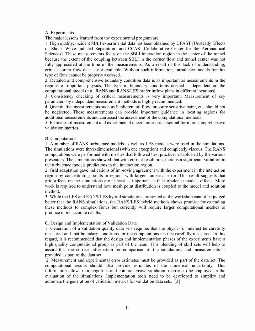
Benek [3], summarizes the major lessons learned from the SWBLI workshop in three
pertinent areas: experiments, computations, and the design and implementation of validation
data. His summary of important findings is quoted below:
11
A. Experiments
The major lessons learned from the experimental program are:
1. High quality, incident SBLI experimental data has been obtained by UFAST [Unsteady Effects
of Shock Wave Induced Separation] and CCAS [Collaborative Center for the Aeronautical
Sciences]. These measurements focus on the SBLI interaction region in the center of the tunnel
because the extent of the coupling between SBLI in the corner flow and tunnel center was not
fully appreciated at the time of the measurements. As a result of this lack of understanding,
critical corner flow data is not available. Without such information, turbulence models for this
type of flow cannot be properly assessed.
2. Detailed and comprehensive boundary condition data is as important as measurements in the
regions of important physics. The type of boundary conditions needed is dependent on the
computational model (e.g., RANS and RANS/LES prefer inflow plans in different locations).
3. Consistency checking of critical measurements is very important. Measurement of key
parameters by independent measurement methods is highly recommended.
4. Quantitative measurements such as Schlieren, oil flow, pressure sensitive paint, etc. should not
be neglected. These measurements can provide important guidance in locating regions for
additional measurements and can assist the assessment of the computational methods.
5. Estimates of measurement and experimental uncertainties are essential for more comprehensive
validation metrics.
B. Computations
1. A number of RANS turbulence models as well as LES models were used in the simulations.
The simulations were three-dimensional (with one exception) and completely viscous. The RANS
computations were performed with meshes that followed best practices established by the various
presenters. The simulations showed that with current resolution, there is a significant variation in
the turbulence models predictions in the interaction region.
2. Grid adaptation gave indications of improving agreement with the experiment in the interaction
region by concentrating points in regions with larger numerical error. This result suggests that
grid affects on the simulations are at least as important as the turbulence models effects. More
work is required to understand how mesh point distribution is coupled to the model and solution
method.
3. While the LES and RANS/LES hybrid simulations presented at the workshop cannot be judged
better that the RANS simulations, the RANS/LES hybrid methods shows promise for extending
these methods to complex flows but currently will require larger computational meshes to
produce more accurate results.
C. Design and Implementation of Validation Data
1. Generation of a validation quality data sets requires that the physics of interest be carefully
measured and that boundary conditions for the computations also be carefully measured. In this
regard, it is recommended that the design and implementation phases of the experiments have a
high quality computational group as part of the team. This blending of skill sets will help to
assure that the correct information for comparison of the simulations and measurements is
provided as part of the data set.
2. Measurement and experimental error estimates must be provided as part of the data set. The
computational results should also provide estimates of the numerical uncertainty. This
information allows more rigorous and comprehensive validation metrics to be employed in the
evaluation of the simulations. Implementation tools need to be developed to simplify and
automate the generation of validation metrics for validation data sets. [3]
12
Another SWBLI workshop was held at the 48th
AIAA Aerospace Sciences Meeting in
2012. Participants in the workshop submitted CFD simulations to four experimentally measured
SWBLIs. Debonis, et al. [5] characterized the CFD predictions, including uncertainty analysis of
the experimental data, the definition of an error metric, and the application of the error metric to
the CFD solutions. For the purposes of the workshop, the SWBLI considered is comprised of an
oblique shock that impinges on a turbulent wall boundary layer, imparting a sudden adverse
pressure gradient onto the boundary layer. As described previously, the abrupt change in
pressure environment causes the boundary layer to thicken up to and possibly including
separation. Experimental data was taken from wind tunnels at the Institut Universitaire des
Systèmes Thermiques Industriels (IUSTI of Marseille, France) and from the University of
Michigan and then modeled by workshop participants with various CFD methods. Last, CFD
results were compared to stereo PIV and LDV experimental data. Furthermore, it is noted that
some of the experimental data used a statistical estimation method {[6], [7], [8]} in order to
estimate uncertainty levels within data.
CFD solutions to the given SWBLI problems were computed using RANS, hybrid
RANS/LES, LES, and DNS simulations. The latter two of which are scale resolving Navier-
Stokes methods [5]. Scale resolving CFD methods are based upon the filtering of finite spatial
regions, resolving portions of turbulence larger than the filter size, and modeling those that are
smaller [9]. These methods can account for things that RANS cannot, such as unsteady heat
loading in unsteady mixing zones and some acoustics applications while also having higher
accuracy than RANS in free shear flows [9] Furthermore, both structured and unstructured grids
were employed. An error metric, E(f), was defined to evaluate simulations and was defined as

13
the difference between CFD and experimental solutions. Further details on this error metric can
be found in DeBonis, et al.’s article [5].
Participants [5] noted several conclusions from the exercises carried out in the workshop.
No single method was identified as being superior over the other methods. There was, however,
an observed opportunity for improvement in the modeling processes. It was noted that RANS
simulations seemed to arrive at the best predictions of turbulent stresses. Furthermore, similar
levels of error were observed for solutions that used both structured and unstructured grids,
suggesting there is little practical difference between grid types. Participants were able to show
that the accuracy of the different modeling methods was not necessarily consistent between
variables of interest; the best predictor of one variable does not mean it will predict other
variables with the same level of success. Debonis et al. [5] states that the turbulence model used
in simulations seemed to have the strongest effect on the accuracy of RANS simulations. Scale
resolving methods (LES, DNS) resulted in similar error levels as RANS, but were better suited to
predicting normal stress levels. As a general conclusion, the participants agreed that additional
research into CFD simulations of SWBLIs is required, and in order to carry out this research,
high quality experimental data that includes effects of sidewalls and corner flow interactions is
required.
Corner Flows
In keeping with SWBLIs, it is important to note that incident oblique shocks cause the
pressure on the boundary layer to change, resulting in thickening of the boundary layer, and
possibly separation, as stated in the sections above. It is impossible to model these flows two
dimensionally, however, since thickening and separation cause fluid flow to move away from

14
sidewalls and toward the centerline plane [10]. Currently, there is a push in the industry for the
development of three dimensional inlet design methodologies that take consideration of the three
dimensionality of high speed flows more fully than the methods currently in use. The complex
flow regimes that result from flows such as boundary layer thickening and corner flow separation
must first be understood in order to successfully achieve this goal [10]. Corner flows pose a
particular problem insofar as there is an oblique shock interacting with a boundary layer, as well
as the two boundary layers of the corner geometry that must interact with one another.
Figure 2: Diagram of Corner Flow Separation with Recirculation Zones (Babinsky, Titchner, [11])
Figure 2 is a diagram depicting a top down view of a test section using a ramp to expand
the test section. In this diagram, it can be seen how the dark grey boundary layer thickens
dramatically upon encountering the expansion ramp and that two recirculation zones then
originate. Flow reattachment occurs after great length of the tunnel is covered. [11]. This may be
a dramatic example of corner flow separation, however, it illustrates the drastic affects that
corner flows can have on overall performance. This is due to the merging of floor and sidewall
boundary layers, which further weakens the flow and makes corner flows especially susceptible

15
to separation. Any weakening of or separation in the flow will cause the stagnation pressure near
surfaces to decrease. This is an undesirable effect for use in wind tunnels, as any variation in
flow properties should be as minimal as possible to keep flow conditions uniform. The length of
the unattached zone, too, is of paramount importance and should be accounted for in this case.
These undesirable facets of corner flows must be simulated with accuracy and consistency if the
next generation of three dimensional supersonic inlets is to come to fruition.
Debonis et al. [5] describe proceedings from a SWBLI workshop in which error in CFD
predictions arose as the strength of shocks increased. That is, as the angle of the shock generator
the workshop participants modeled increased, the error in simulations did too. Furthermore,
Hirsch, [12] states that CFD simulations tend to underpredict the size of the SWBLI region.
Related to the underprediction of the SWBLI regions are the axial location where shocks interact
with the boundary layers, with the simulations generally showing the shocks hitting the walls at a
later axial position than experimentally recorded data [12].
Having a wind tunnel with the most predictable, reliable test section flow can certainly
help to alleviate some of the negative effects that might arise when testing geometry in which
corner flows are present. Understanding how corner flows behave and the ways in which
boundary layers interact with the environment must be taken into account in these sorts of
applications.
Data Validation
An important aspect of studying CFD methods and uses is how to characterize data from
simulations; is the simulation accurate and does it agree with real world applications (such as
experimental scenarios)? CFD data must be validated in order for it to be put to good use and to
answer these questions confidently.
16
As Benek reported from the findings of the AIAA Shock Boundary Layer Interaction
Prediction Workshop [3], an important lesson learned from the SWBLI workshop is in regards to
the design and employment of experimental procedures geared toward collecting data sets for
use in CFD data validation. A typical experimental procedure is generally focused on a particular
region of interest, which is both logical and efficient for experimental uses. Validation data sets
must include measurements of regions that are not typical areas of focus in order to fully
describe the characteristics within an experimental test. Every region in a test section may not
always be of primary interest, and as such may not lend much information to experimental tests.
However, these regions are instrumental for use in validating numerical simulations [3]. In this
fashion, validation data sets can provide CFD analysts a standard with which to determine the
predictive power of numerical models.
As with the creation of any standard industry model for practice, the validation sets must
be subject to consistency checks by measuring desired properties with numerous and alternative
data collection methods. Estimates of measurement uncertainties for both the experimental and
numerical simulations must be taken into consideration when comparing CFD to experimental
data. Debonis, et al. [5] describe how PIV and LDV measurements can be used in conjunction
with an error metric/uncertainty analysis in order to show the validity of CFD data. Numerical
simulations must match validation data as closely as possible to make the best CFD-to-
experimental comparisons [3].
Periodic activities, such as those at the various SWBLI workshops, give engineers the
opportunity to explore these aspects of data validation; the more understanding of how CFD
corresponds to experimental data, the more trust can be laid in future numerical simulations.
Indeed, the Air Force Collaborative Center for Aeronautical Sciences has compiled a database of

17
experimental measurements for use in assessing CFD simulations, as mentioned by Eagle,
Driscoll, and Benek [10].
The fact that past simulations have been carried out and compared with data validation
sets for similar RANS type CFD tests for the specific University of Michigan asymmetric wind
tunnel in question throughout this document lends credence to the methodology used in these
proceedings.
Physical Wind Tunnel
The wind tunnel that simulations in this document are based upon is an existing
supersonic wind tunnel at the University of Michigan. This tunnel, shown in the Figure 3 below,
is an asymmetric, converging-diverging, “suck down” wind tunnel. The suck down setup allows
for constant stagnation temperatures/pressures, and Mach numbers throughout a test run [13].
Figure 3: Side View of Experimental Wind Tunnel, Sidewall Removed (Lapsa, [13])
18
The tunnel has optical access on three sides of the test section, which allows for various
diagnostics to be run, such as SPIV, etc. According to Lapsa [13] the asymmetric wind tunnel
allows for two advantages to be present in the test section. First, having the bottom plane of the
test section effectively acting as a flat plate, a compressible boundary layer is formed with
decreased pressure gradient effects, resulting in velocity profiles similar to a zero pressure
gradient profile. Second, the nozzle may be reconfigured to reach several different desired Mach
numbers. The test section in question measures 2.25 wide by 2.75 inches tall [13] and 36 inches
long [14]. The converging portion of the nozzle is 12.088 inches long. The beginning of the test
section location (discussed in greater detail in Chapter 4) is 28.292 inches downstream of the
throat and 40.38 inches downstream of the nozzle inlet [15]. The throat height is 1.887 inches.
For the purposes of this document and the studies therein, the experimental Mach number
through the test section in question is 1.8.
Mitigation of Negative SWBLI Effects
Inherent with SWBLIs is the desire to mitigate the adverse effects imposed by the
interactions. Loss of efficiency, boundary layer separation, boundary layer thickening, etc. are
but a few of the adverse effects present with SWBLIs. Over the years, several different
techniques have been developed to mitigate the adverse characteristics that arise with the
presence of SWBLIs. The methods used in several of these techniques will be outlined below.
Bleed Air
Reducing the size of the boundary layer before it is exposed to any sort of shock waves is
one method that is used to reduce the effects of SWBLIs. Making the boundary layer of a system

19
thinner will reduce the effect that the low energy of the boundary layer has on the rest of the
system. As Hazen [16] states, suction may be applied to the boundary layer, through porous
surfaces or a series of slots. This causes some of the slower moving boundary layer to be bled
out, reducing the overall thickness of the boundary layer which further results in more stability
near surfaces. This can help to delay the transition to turbulent flow in cases where transitional
flow is present.
This method may be applied to both internal and external structures in a similar fashion.
Figure 4 shows the same airfoil before and after suction was used on the outer surface. Figure 4a
shows a mostly turbulent boundary layer along the majority of the length of the upper wing
surface. Figure 4b shows that using suction reduces the boundary layer, which now remains
laminar over the upper wing surface. Suction/bleed air can also help to keep boundary layers
over surfaces from separating at high angles of attack. With the use of suction on an airfoil it is
possible to keep flow attached to the surface at points well beyond typical stall angles [16].
Hazen [16] also demonstrates how this method affects momentum in the flow. Without
the use of suction, wakes are broad, which is indicative of high amounts of drag. Adding suction,
however, causes wake sizes to decrease along with thinning of the boundary layers. Smaller
wakes translate to less drag from momentum losses affecting flows over surfaces. The number of
bleed air slots and/or porous surface configuration depends on flow characteristics, location,
amount of suction needed, etc. Clearly, much time and study is necessary to tailor use of this
method for a particular application and is an important field unto itself.

20
a)
b)
Figure 4: Boundary Layer Mitigation with Suction.
a) No suction, turbulent boundary layer along wing surface. b) Suction used. Boundary layer remains laminar along wing surface. (Haxen, [16])
Specifically, according to Harloff and Smith [17] boundary layer bleed is used in
supersonic inlets to avoid boundary layer separation caused by the adverse pressure gradient
involved with SWBLIs that result in total pressure loss along the subsonic diffuser. The amount
of bleed air required for certain circumstances can be determined based on a boundary layer
incompressible shape factor, Hi. Computer simulations to further evaluate bleed configurations in

21
supersonic inlets take advantage of classical supersonic nozzle equations, Darcy’s law for porous
plates, and the specification of the local sonic flow coefficient as a constant [17].
Included with bleed or suction air systems, however, is an inherent loss of performance.
As is outlined by Anderson, et al. [4], bleed air does not typically rejoin the main inlet flow,
meaning the mass flow captured during the bleeding process is lost. Rather, it is often vented into
the atmosphere through exit holes, causing a further increase in drag. A larger nacelle may be
needed on engine inlets as compensation for lost mass flow, which increases both drag and
weight of the aircraft. Additionally, boundary layer bleed is generally vented into the
atmosphere, resulting in yet even more reduction in aerodynamic performance.
There have been bleed type boundary layer mitigation systems since the inception of high
speed aircraft. As shown in Figure 5, the Bell P-59 incorporated a simple slot, through which low
momentum flow from the fuselage boundary layer flow would be kept from entering the engine
inlet. Similar such devices can be seen historically on many different aircraft, such as the
Lockheed F-80, Northrup F-89, the Convair F-106, etc., and are still used on modern day
supersonic aircraft [18].

22
Figure 5: P-59 Internal Boundary Layer Diverter (Surber and Tinnaple, [18])
As aircraft design progressed, however, bleed slots, such as those used on the P-59, began
to be used in conjunction with other boundary layer mitigation systems, such as vortex
generators. [18].
Vortex Generators
Instances when SWBLIs cause separation in the boundary layer can result in shock
oscillations throughout internal flows. To control the amount of separation experienced in
situations such as these, there have been methods developed that employ the use of vortex
generators. These systems introduce streamwise vortices into the flow that are injected by air jets
[19]. Typical jet configurations are inclined at an angle 45º normal to the flow plane and oriented
at 90º in the plane parallel to the flow. These vortices affect the static pressure downstream of the
shocks, which helps to reduce the amount of separation in the boundary layer. Jets cause the
velocity downstream of shocks to increase relative to jet-free flows, which corresponds to a

23
decrease in static pressure. A lower pressure generally helps to decrease the amount of separation
in the boundary layer [19]. This in turn decreases the effects caused by adverse pressure gradient
in the direction of the flow. Furthermore, these vortices allow for higher momentum fluid to
enter the lower sub-layers of the boundary layer, helping to negate the low momentum fluid
found near surfaces, further reducing separation [19].
Vortex generators are a viable way to deal with alleviating problems that arise due to low
momentum flow since boundary layers are comprised of relatively low momentum flow in the
areas near surfaces. Vortex generators help to increase the energy found within boundary layers
by mixing high momentum fluid from outer flow with the relatively low momentum flow found
closer to the surface [16]. Higher momentum means higher velocities closer to surfaces, which
means thinner boundary layers and more uniform flow [19]. Figure 6 below shows a comparison
of non-dimensionalized velocity profiles with and without vortex generating air jets. This clearly
depicts how the presence of jets helps to increase boundary layer velocity.
Figure 6: Illustration of VG Air Jets on BL Velocity (Szwaba, et al. [19])
24
Microramps
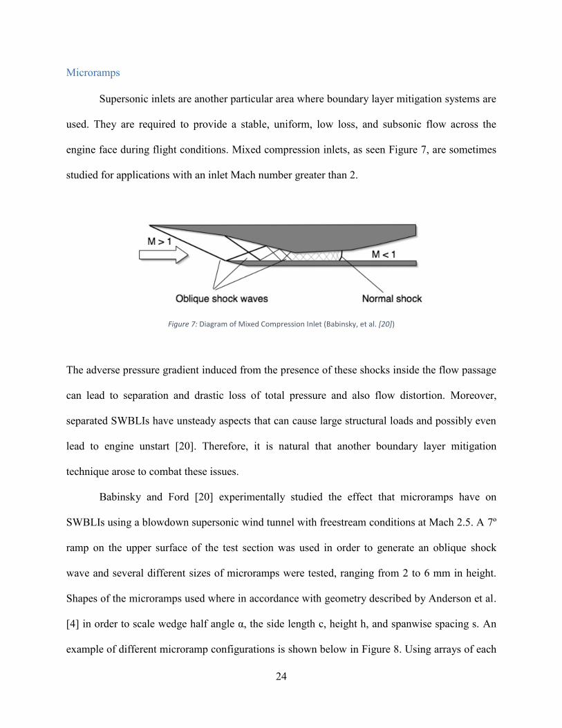
Supersonic inlets are another particular area where boundary layer mitigation systems are
used. They are required to provide a stable, uniform, low loss, and subsonic flow across the
engine face during flight conditions. Mixed compression inlets, as seen Figure 7, are sometimes
studied for applications with an inlet Mach number greater than 2.
Figure 7: Diagram of Mixed Compression Inlet (Babinsky, et al. [20])
The adverse pressure gradient induced from the presence of these shocks inside the flow passage
can lead to separation and drastic loss of total pressure and also flow distortion. Moreover,
separated SWBLIs have unsteady aspects that can cause large structural loads and possibly even
lead to engine unstart [20]. Therefore, it is natural that another boundary layer mitigation
technique arose to combat these issues.
Babinsky and Ford [20] experimentally studied the effect that microramps have on
SWBLIs using a blowdown supersonic wind tunnel with freestream conditions at Mach 2.5. A 7º
ramp on the upper surface of the test section was used in order to generate an oblique shock
wave and several different sizes of microramps were tested, ranging from 2 to 6 mm in height.
Shapes of the microramps used where in accordance with geometry described by Anderson et al.
[4] in order to scale wedge half angle α, the side length c, height h, and spanwise spacing s. An
example of different microramp configurations is shown below in Figure 8. Using arrays of each

25
sized microramps Babinsky et al. [20] used laser Doppler anemometry (LDA) to record fluid
velocities along the tunnel test section.
Figure 8: Microramp Configuration (Babinsky, et al. [20])
Babinsky et al. [20] were able to demonstrate that the size of the microramps used did not
have an effect on fundamental flow characteristics; each configuration/size tested resulted in
essentially the same flow characteristics of oblique shocks beginning at the leading and trailing
edges of the ramp, as shown in Figure 9. An important conclusion the authors reached is that
each of the arrays tested was able to decrease the influence the adverse pressure gradient had on
downstream flow, as shown by decreases in pressure when compared to vortex generator free
configurations. Together, the lessened effects of the adverse pressure gradient and decrease in
pressure suggests a reduction in the amount of separation caused by SWBLI effects has occurred
[20].

26
Figure 9: Microramp Schlieren Photo and Surface Oil-Flow Visualization (Babinsky, et al.[20])
This process can be illustrated visually, as shown in Figure 10. The ramps cause vortices
to appear near the boundary layer, which help to increase movement of high momentum fluid
near the low momentum boundary layer area. As these different momentum fluids interact with
one another, higher momentum is imparted onto the boundary layer from the vortices, dissipating
the affects that the low momentum boundary layer has as the fluid moves downstream [20].
This concept is similar to that of bleed holes in that a similar curvature is created in the
flow. Vortex generators cause a system of higher momentum regions to propagate through the
flow while interacting with lower momentum fluid close to surfaces. This interaction causes
mixing between the two levels of momentum making the higher momentum fluid to “curve”
toward surfaces, effectively decreasing boundary layer thickness. Bleed holes create a similar
curvature of higher momentum flow toward surfaces by bleeding some low momentum fluid
away and enhancing mixing with what remains.

27
Figure 10: Low Momentum Region Dissipating (Babinsky, et al. [20])
Why Mitigation Matters/SWBLI Modeling Tie-In
It is important for engineers to understand the impacts that SWBLI mitigation techniques
have on both SWBLIs and the effects on overall aircraft performance. A deep understanding of
the ways in which SWBLIs are mitigated allows for continued improvements on existing and
future aircraft. Hand in hand with this are the ways in which supersonic applications are tested; a
better understanding of the concepts discussed above will allow for better implementation and
use of test facilities. Also inherent within this continual process of improvement is the CFD work
that will be conducted. Experimental and numerical methods must be used together to improve
one another; understanding the physical effects that SWBLI mitigation techniques have on
aircraft performance will enable all the more accurate CFD models which will corroborate and
enhance physical and experimentally tested models.
Ramp
Vortex
Low
Momentum
Region

28
Design of Supersonic Wind Tunnels, a Historical Perspective
Supersonic nozzles and wind tunnels have been in use for over a century. As summarized
by Anderson [21], the first supersonic nozzle was made by de Laval in the late 1800’s, with the
first supersonic wind tunnel (Mach 1.5) following in 1905 (built by Prandtl for studying the
movement of sawdust through sawmills), and the first practical supersonic wind tunnel was made
by Busemann in the mid 1930’s. With a history of this length it is only fitting that the design of
these tunnels and nozzles was very different in the early years. Due to computational limitations,
early supersonic applications were often carried out with the assumption that the flow was two
dimensional and that the fluid was inviscid. Modern methods have moved beyond these
assumptions, but early forms of supersonic nozzle design used these simplifications for ease of
calculations. Several such method of design will be considered below.
As described by Anderson [22], supersonic converging diverging nozzles are comprised
of a converging section upstream in which the flow is accelerated to sonic speed. The narrowest
part of the converging section, the throat, is the location at which the speed of sound is achieved.
A “sonic line” is typically noted as being located at the throat. Sonic lines are slightly curved due
to the multidimensionality of subsonic flow that is converging but are often depicted as being a
straight vertical line. The nozzle contour begins to diverge following the throat and downstream
of the sonic line. The diverging section experiences further increases in fluid velocity and
expansion waves are generated that begin to propagate downstream. The expansion waves reflect
off opposing walls and must be “straightened” by the nozzle walls to bring the flow back to
parallel with the centerline.
Puckett [23] describes an early method of supersonic nozzle design based upon Prandtl
and Busemann’s 1929 method of characteristics in his paper Supersonic Nozzle Design (1946).

29
The method of characteristics is applied to incompressible, inviscid fluid in two dimensions
using two dimensional flow fields through which supersonic velocity is represented
approximately by quadrilaterals of constant velocity and pressure and separated by lines that
represent waves in the flow. Increasing the number of these quadrilateral areas will increase the
accuracy of calculations. Equations of fluid motion are used in this method to graphically
determine how flow characteristics change through geometry across different waves.
Conservation of mass and Newton’s Second Law are used to determine local speeds of sound,
Mach angles, etc. and Prandtl-Meyer conditions are utilized to arrive at fluid properties in each
region of interest. In this manner, the method of characteristics may be applied in order to
compute nozzle wall shapes in order to arrive at uniform and parallel flow velocity across wind
tunnel test sections.
The specific equations that govern the method of characteristics may be found in
Puckett’s text [23] but will only be conceptually summarized in this document. In supersonic
flow, when the moving fluid encounters a change in geometry there will be a corresponding
expansion or compression wave that accompanies. Essentially, conservation of mass, Newton’s
Second Law, and energy equations are applied to known flow inlet conditions at locations
beginning with a change in flow angle. The relationship between the change in speed and change
in flow direction/angle may be determined as these equations are applied (and assuming that
flow crossing waves is isentropic) the. It is possible to calculate flow properties through
consecutive changes in geometry, as shown Figure 11 below [23], by recalling how Mach
number is used in the Prandtl-Meyer function. Waves can be seen originating at the point each
angle change begins.

30
Figure 11: Flow Direction through Angle Changes (Puckett, [23])
The basic way supersonic nozzles have historically been designed, by calculating flow
properties along angle changes and across waves with the number of straight sections between
waves being sufficiently large enough to approximate a curve, has remained an industry
standard. With this in mind, there are two scenarios that must be acknowledged and understood
in order to adequately design a nozzle: the intersection of two waves and the intersection of a
wave and wall. As Puckett describes, for two waves that intersect as shown in Figure 12, it
should be noted that the wave W1 was produced by an initial deflection of dθ1 and will go on to
produce a deflection of dθ1 after it passes W2. The same deflection relation is found with W2 and
dθ2, as well. When this method was developed, extensive sets of tables were employed such that
calculating flow properties from region to region (such as M1 to M4 below) could be done at a
readily computed speed by using the method of characteristics [23].

31
Figure 12: Intersecting Waves (Puckett, [23])
The intersection of walls and waves produces a reflection of said wave that must be
propagated in a direction parallel to the bounding wall. Accounting for waves in this manner is
known as “cancelling” and as shown in Figure 13. Cancelling is used to help return flow parallel
to the nozzle centerline after the expansion zone. This helps to ensure uniform flow in the test
section [23].
Figure 13: Intersection of a Wave and Wall (Puckett, [23])
Puckett [23] describes two general methods for achieving desired supersonic nozzle
operating conditions. The first method is known as maximum expansion design, wherein the
initial shape of the expansion section is arbitrary up to the point where the maximum expansion
angle occurs. Figure 14 below illustrates this concept (from the nozzle centerline up). In this

32
example, the short, straight line sections past the throat are arbitrarily increased by 2° each up
until the arbitrary maximum angle of 8° is reached. Past this, the nozzle profile must begin to
turn the flow back toward parallel with the centerline, which is achieved by decreasing the
inclination of the outer wall by 2° successively at each instance where a reflection wave hits the
wall. The value of 2° is used to “cancel” the effect of the original 2° successive deflections found
in the expansion zone. This is repeated until the flow is uniform and parallel to the centerline
[23]. It should be noted that both the waves and wave reflections expand the flow, while the
wave reflections are used in such a way to straighten the expanded flow back to parallel/uniform
flow.
Figure 14: Illustration of Maximum Expansion Design (Puckett [23])
Following this, the method of characteristics described above is used to calculate flow
properties from region to region. Furthermore, it is noted that the maximum allowable expansion
angle for a supersonic nozzle is equal to one half of the Prandtl-Meyer angle that corresponds to
the final Mach number. The method of characteristics may be used in reverse with the Prandtl-
Meyer angle to determine the shape of the expansion zone and remaining nozzle profile for use
in real world scenarios the desired final Mach number is usually known [23].

33
Puckett’s second design method is known as less than maximum. This method uses an
expansion angle less than the maximum that is governed by the Prandtl-Meyer angle for a given
ending Mach number. However, using a less steep angle will require more nozzle length to reach
the same level of expansion to arrive at the desired Mach number. As Figure 15 shows, the final
Mach number is the same as in Figure 14, but the nozzle profile is quite different. [23]
The maximum expansion method results in the shorter nozzles than the less than
maximum method, but sometimes results in less uniform flows. Less than maximum nozzles
have more uniform flows but are more susceptible to boundary layer losses due greater lengths.
Thus it is reasonable to use an angle that is slightly less than the maximum permitted by the
Prandtl-Meyer relation [23].
Figure 15: Less Than Maximum Expansion (Puckett, [23])
In summary of Puckett’s nozzle design procedure, the five following steps are listed (and
can be found in [23]). Following these procedures should ensure that flow is sufficiently
expanded and turned back to parallel for a given scenario. There should be characteristic lines of
constant magnitude at all locations after the point at which flow returns to parallel, signifying
parallel/uniform flow has been reached.

34
Table 2: Puckett's CD Nozzle Design Steps (Puckett, [23])
1 Determine the speed index of the desired design Mach number (using values found on a
functions of expanding flow table)
2 Determine the maximum permissible expansion angle using the equation ,
and choose an expansion angle equal to or less than this.
3 Choose an expansion curve from the throat to θa
and divide this into suitable straight
segments, where the disturbance wave strength might be 1 or 2º depending upon the
desired accuracy.
4
Construct the expansion waves produced by this section and their
intersections/reflections from the center line. If θa is less than θmax, determine the
necessary number of reflections from the wall using the number of reflected waves
equation,
.
5 Construct the section canceling all expansion waves and producing a parallel flow.
For the purposes at hand, the fifth step is perhaps the most crucial, for it is this step that
ensures the flow returns to parallel. Without accuracy at Step 5, uniform flow will not be attained
in the test section and the integrity of the flow may not be adequate enough to yield accurate
work.
Anderson [22] describes yet another method of designing supersonic nozzles, wherein the
length is kept short for design purposes, called minimum length nozzles. This configuration
employs an expansion section that emanates from a sharp corner throat at which a Prandtl-Meyer
wave is centered upon [22]. The method of characteristics is employed for calculating the
contour details. The resulting length of the nozzle is such that it corresponds to the minimum
possible length for which a shock free, isentropic nozzle can be obtained. Designing a contour
that is not adequately long will result in shocks occurring in the nozzle section of the contour
[22].

35
This type of nozzle is well suited for applications where length is of paramount concern,
such as rocket nozzles, and for non-equilibrium flow used in rapid expansion configurations
[22]. Anderson’s method differs from Puckett’s [23] insofar as the final results of Puckett’s two
methods arrive at configurations of greater length and have a more gradual expansion section.
These methods take do not take fluid viscosity into account, thus the solutions arrived at
will be approximations. It was convention in Puckett’s time to treat the core of the flow through
supersonic nozzles as inviscid, with a thin viscous boundary layer lining the walls of the nozzle.
The boundary layer is slower than core flow and thickens as it moves downstream. Puckett
describes how engineers at the time treated the boundary layers as “effective walls” which are
governed by the displacement thickness of the boundary layer [23]. Displacement thickness is a
function of the axial position and is useful in keeping the mass flow rate the same between a
designed nozzle configuration and that which arises due to the effective walls [24]. To keep mass
flow rates the same, the displacement thickness is used to re-compute the design parameters in
Figure 16: Anderson's Minimum Length Nozzle (Anderson, [20])

36
order to calculate how much the flow must be displaced to achieve the same mass flow rate
through the effective walls as in the designed physical boundaries [23].
In this manner, the fluid was treated as a perfect, inviscid flow passing between the
boundary layer-created effective walls rather than the physical contour walls. Figure 17
illustrates the effective wall assumption as governed by the displacement thickness. Engineers
would increase the size of the physical walls relative to the displacement thickness such that the
effective walls would be close to the designed profile necessary to achieve desired mass flow
rate conditions in order to counter the narrowing effect produced by the boundary layer.
Typically, the top and bottom physical walls were diverged at rates close to 0.007-0.010 inches
per inch of length in Puckett’s time. This roughly accounted for boundary layer thickening
and/or displacement thickness effects in the downstream direction [23].
Figure 17: Boundary Layer Effective Walls (Puckett, [23])
The essence of how supersonic nozzles and wind tunnels are designed has remained the
same through the years. The advent of computers has meant that a much greater level of
accuracy is possible in current design than in decades past. The method of characteristics is still
used but the days of hand calculations and reference tables are gone. The resolution with which
modern computers are able to make the same calculations has increased dramatically, and will

37
likely continue to do so. CFD further allows for the automatic coupling of both inviscid and
viscous solutions methodologies, enabling the method of characteristics to be used in
conjunction with displacement thickness, resulting in much more accurate results than in the
past.
Review of Asymmetric Wind Tunnels/Nozzles
Asymmetric wind tunnels are sometimes an attractive alternative to the conventional
symmetric kind, especially where cost and mechanical simplicity are of concern. The following
section will detail certain aspects regarding the design of asymmetric supersonic CD nozzles,
including the theory, advantages/disadvantages, and methods of design.
Similar to axisymmetric supersonic CD nozzles, asymmetric CD nozzles have a
converging section upstream where flow is accelerated to sonic velocity at the throat. This is
followed by a diverging section for flow to further expand and increase velocity. The methods
shown in the preceding section for use with axisymmetric supersonic CD nozzles, however, are
not as well suited to asymmetric nozzle configurations, which may utilize fairly different upper
and lower wall contour profiles. Several methods that have been tailored exactly for these types
of scenarios and nozzle configurations are outlined below.
Although not as common as symmetric nozzles, there has been interest in asymmetric
nozzles and wind tunnels for decades; adjustable asymmetric supersonic nozzles have existed
since at least the early 1950’s [25] and have been used for various applications since. Liepman
[26] describes asymmetric tunnels as being more mechanically simple than axisymmetric. For
example, continuous variation in Mach number is easily attained with sliding block
configurations (discussed further below) which can be programmed to change Mach number

38
with time for use in simulating different flight cycles and operating conditions. Continuous wall
curvature found in some asymmetric nozzles can help to lessen the difficulties related to points
of inflection and test section junctures that are present in traditional nozzle configurations.
However, at least in the early days of Liepman, asymmetry in nozzle configuration tended to
mean that nozzle length would be approximately twice that of traditional nozzles.
Allen was an early pioneer in asymmetric supersonic nozzle work and described in 1948
[25] the development of an asymmetric supersonic wind tunnel with adjustable, non-flexible
walls. In any wind tunnel it is important to have sufficiently small velocity gradients normal and
parallel to the test section flow in order to attain accurate results. This requires the ability to
adjust test section airspeed whether for a sub or supersonic applications. This is easily
accomplished by increasing the speed of the driving fan/compressor in subsonic applications.
Since fluid speed beyond the throat in supersonic tunnels is dependent on the ratio of the axial
position to the throat area and the pressure ratio P/Po at these locations, adjusting the speed of the
test section fluid must be accomplished by changing the shape of the nozzle, rather than
increasing the speed of driving fluid. The desire to have flow that meets these requirements at a
varying range of Mach numbers led Allen to develop a new type of tunnel, as the previous
methods for achieving variable Mach numbers (discussed in detail below) were deemed too
cumbersome and unrealistic for continued use.
Allen describes several methods for attaining variable Mach numbers [25], each with
differing drawbacks, which have been used to change flow characteristics in asymmetric
supersonic wind tunnels: interchangeable nozzle shapes, flexible walled variable geometry
nozzles, and plug type nozzles. Interchangeable nozzle shapes are cumbersome and limited by
the number of nozzle configurations available, but have the advantage of being mechanically

39
simple. Flexible walled variable (see Figure 18a) nozzles use thin walls that can be adjusted
using a series of jacks which tune the nozzle shape to desired levels. However, these jacks
require a large number of mechanical components that are subject to high stresses and flow
leakage, which requires extensive safety measures to be taken. Plug type nozzles (see Figure
18b) use a “trumpet shaped duct” with a plug that is inserted that that creates two small throats.
The plug can be moved axially to change flow speeds in the test section. However, a viscous
wake trails the plug and propagates through test section, making model placement difficult, and
it became doubtful that boundary layer correction (porous suction removal, etc.) would be
sufficient to correct this [25].
a)
b)
Figure 18: a) Flexible Walled Variable Mach Number Nozzle and b) Plug Type Variable Mach Number Nozzle (Allen, [25])

40
Allen’s [25] proposed third solution is an asymmetric nozzle, like the one depicted in
Figure 19, which is composed of a fixed upper wall and a horizontally translatable lower wall
which is used to change throat position and area. It strives to make up for the shortcomings of
mechanical complexity and undesirable flow conditions found in the methods above. It was
shown that asymmetric nozzles of this kind can successfully produce viable test section flows at
Mach numbers between 1.1 and 2.0. However, pressure gradients were found to exist in the test
sections at Mach numbers higher than 2.0.
Figure 19: Allen's Asymmetric Nozzle (Allen, [25])
Allen [25] describes how early iterations similar to Figure 19 were arrived at by simply
cambering the contours of already existing axisymmetric nozzles which were known to be
satisfactory at a desired operating condition. As this work progressed, the method of
characteristics was utilized to see how changes in shape would improve the desired flow.
Schlieren photographs were used to observe flow within the test section, and it was found that
41
shortening the overall length of the asymmetric configuration made the flow more likely to be
unsatisfactory [25].
Clearly, the early developments made by Allen were not suitably efficient or accurate
enough for wide scale implementation as a common method of design. Syvertson and Savin [27]
demonstrated two methods for use in designing asymmetric supersonic wind tunnels for use with
varying Mach numbers that were more straightforward than Allen’s method. The goal of
Syvertson and Savin’s research was to use what Allen [25] had developed and have more
consistent, uniform test section pressure characteristics. Two such methods were developed for
use in Allen-style asymmetric nozzles: one for use with Mach numbers below 3.0, and the other
for Mach numbers above 3.0.
The first such method, for use approximately at or below Mach 3, determines
downstream portions of tunnel walls necessary for uniform exit flow first, followed by
calculating the flow field characteristics that must occur between these wall portions for uniform
exit flow to exist, and finally calculates the portions of the upstream walls’ shapes to facilitate
the flow fields in the downstream portions of the tunnel. Detailed appendices and a greater
description of this process may be found in Syvertson and Savin’s 1951 publication [27]. Using
these three steps in conjunction with Prandtl and Buseman’s [28] method of characteristics,
Syvertson and Savin have shown that exit flow can be made nearly uniform through a range of
Mach numbers that vary from slightly below to slightly above the desired design Mach number.
This non-iterative approach can be used to theoretically create uniform exit flow for use in an
asymmetric supersonic wind tunnel at two different Mach numbers [27]. It is further stated that
in order to minimize irregularities in the flow when running at off design conditions that the
position of the minimum section between the walls should traverse continuously upstream along

42
the upper and lower contours as the exit Mach increases. To do this, neither wall should contain
inflection points, have finite curvature radii, and local radius of curvature must always be lower
than that of the upper wall (to guarantee only one minimum exists). Characteristic nets are used
in order to determine the shape at desired conditions (see Syvertson and Savin [27] for a more
detailed description of characteristic nets and the uses thereof).
For Mach numbers approximately greater than 3, Syvertson and Savin employ a design
method that utilizes an averaging process which results in asymmetric nozzles that have nearly
uniform test section and exit flow. This approach, described in detail in Syvertson and Savin’s
1951 publication [27], is similar to the under 3 Mach design process described above, except that
the flow is made to not reach Prandtl-Meyer flow at the same point along the nozzle. Rather, the
shape of the upper wall is changed to provide for more uniform exit flow, and the characteristic
net is recalculated. Then, an arithmetic mean of the resulting contour extremes is taken to
determine contour shape. Resulting test section and exit flow conditions should be nearly
uniform. This process may require several iterations before arrival at the desired results [27].
Syvertson and Savin were therefore able to demonstrate two methods, non-iterative and
iterative, respectively, for generating theoretically uniform exit flow over a small range of
desired Mach numbers by way of curving nozzle contours. The way in which these contours
were used in conjunction with the method of characteristics means that an inclined or curved
sonic line is present during calculations though Syvertson and Savin [27] do not consider this an
“essential feature” of the design process.
Liepman [26] discusses another method which can be used to design two dimensional
asymmetric supersonic nozzles (similar to the types of asymmetric nozzles described by Allen
[25]). Until Liepman’s developments were demonstrated, the main way of designing asymmetric

43
nozzles was by way of implementing the method of characteristics graphically, like those
developed by Allen [25] and Syvertson and Savin [27]. Liepman states that since graphical
methods are not accurate enough to result in sufficiently high quality flow through test sections
that an analytic approach must be found. This analytic method is based upon symmetrical nozzle
design, and has the advantage of not needing to make any assumptions with respect to the sonic
line (as the graphical approaches do). However, Liepman’s analytic method still requires an
iterative process (although substantially shorter than the graphical methods). [26]
Specifically, Liepman’s analytical method [26] is built upon the derivation of the basic
equations for irrotational and steady flow of an isentropic, compressible fluid as it moves
through an asymmetric nozzle contour that has been divided into a subsonic region, supersonic
expansion/reflection region, a supersonic simple wave region, and the test section. Liepman’s
derivations are lengthy and may be found in detail in his 1953 Air Force document [26]. Upon
proving the derivations therein, Liepman showed an analytical approach to design was possible.
Liepman goes on to recommend that boundary layer corrections should be implemented in order
to ensure that expansion waves and the effective walls of the tunnel interact in such a way that
the desired angular relations remain valid.
Burbank and Byrne [29] demonstrated a method of designing an asymmetric, fixed
geometry nozzle with variable Mach number in 1953. This work began with a nozzle
configuration similar to that described by Allen [25]; upper and lower blocks are used to create a
non-flexible nozzle contour where one block may be translated in a direction parallel to the test
section flow in order to change the contour between the nozzle blocks, thus changing flow
characteristics in the test section. Burbank and Byrne’s method utilizes a characteristic net not
unlike those described in earlier sections, but with the design condition that the sonic line coming
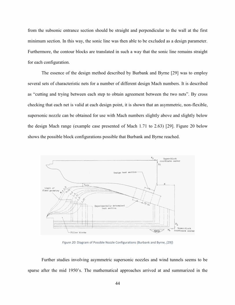
44
from the subsonic entrance section should be straight and perpendicular to the wall at the first
minimum section. In this way, the sonic line was then able to be excluded as a design parameter.
Furthermore, the contour blocks are translated in such a way that the sonic line remains straight
for each configuration.
The essence of the design method described by Burbank and Byrne [29] was to employ
several sets of characteristic nets for a number of different design Mach numbers. It is described
as “cutting and trying between each step to obtain agreement between the two nets”. By cross
checking that each net is valid at each design point, it is shown that an asymmetric, non-flexible,
supersonic nozzle can be obtained for use with Mach numbers slightly above and slightly below
the design Mach range (example case presented of Mach 1.71 to 2.63) [29]. Figure 20 below
shows the possible block configurations possible that Burbank and Byrne reached.
Figure 20: Diagram of Possible Nozzle Configurations (Burbank and Byrne, [29])
Further studies involving asymmetric supersonic nozzles and wind tunnels seems to be
sparse after the mid 1950’s. The mathematical approaches arrived at and summarized in the

45
section above remain sound to this day, however, the computational resolution possible for the
design process has increased greatly. No longer are hand calculations or tables required to arrive
at accurate and reliable configurations; with the technology present today, it is possible to design
asymmetric nozzles and wind tunnels for use in supersonic applications with a much greater
degree of accuracy than in the early years of design.
Implications for Current Research
The methods described above shed light onto why non-uniform flow might arise in an
asymmetric supersonic wind tunnel. Symmetric configuration design methodology takes the
displacement thickness of the system into consideration. This ensures that the mass flow rates of
the system are in accordance with what is necessary to achieve the desired flow characteristics
and likely achieve uniform flow. The University of Michigan asymmetric wind tunnel
considered here, however, has a lower wall that remains parallel to the x-axis for the whole span
of the tunnel. This means that the displacement thickness is not taken into account, which calls
the reliability of the test section flow into question. Minute differences in flow characteristics
resulting from unaccounted displacement thickness can affect the integrity of the flow.
Moreover, cancelling effects may not be achieved due to the smaller effective walls induced by
the boundary layer.
The upper wall of the UM tunnel may still be adjusted for boundary layer and
displacement thickness effects, but if the lower wall is to remain parallel to the x-axis it cannot
be adjusted. If it is desired to reconfigure the lower plane to account for displacement thickness,
a new lower wall would have to diverge away from the x-axis by a certain amount in order to
fully compensate for displacement thickness effects. The resultant lower plane would angle away
46
from the tunnel’s centerline, with the angle increasing as axial position increases due to the fact
that displacement thickness is dependent on axial position, getting thicker as position increases.
Any sort of deviation away from parallel in the lower wall would make it impossible for the flow
to return to parallel, instead resulting in flow that continually has flow angle changes. As it is
currently configured, the UM tunnel keeps the parallel lower plane, meaning that the
displacement thickness acts as a non-parallel effective boundary that grows in thickness along
the tunnel, resulting in flow that is always turned slightly away from parallel.

47
3. Methodology
Newton’s second law and the laws of conservation of mass and energy are the base upon
which computational fluid dynamics is built. The Navier-Stokes equations were developed using
these fundamental aspects of fluid motion and strive to express how the velocity, density, and
temperature of fluids in motion behave with respect to time.
Navier Stokes
It should be noted that the equations presented herein are displayed in differential form,
meaning it is assumed that the fluid in question exists in a continuum. However, the
computational capabilities in today’s CFD industry do not facilitate that application of the
Navier-Stokes equations to every single point in space found in the continuum. Rather, CFD uses
the Navier-Stokes equations to obtain numerical solutions for discrete points. The equations
below are in vector form as seen in Anderson et al.’s text [30] in terms of compressible flow
without external heat and/or body forces for Cartesian Coordinates.
(1)
(2)
(3)

48
(4)
(5)
(6)
(7)
49
Equation (1) shows the collection of all the necessary partial differential equations
displayed together in vector form. The U array shows the variables that CFD initially computes.
E, F, and G are the directional components of the equation sets. The first equation in E, F, and G
represents the conservation of mass equations. The second, third and fourth equations of E, F,
and G represent the separate components of Newton’s Second Law (the momentum equation).
The last equation found in E, F, and G represents the energy equation. When computed together,
this set of equations represents the partial differential equations necessary to compute the Navier
Stokes equations in a vector form. Equation (6) represents the different possible shear stresses
necessary to complete E, F, and G [31].
Equation (7) is the equation of state, which is used in order to close the system of
governing equations by connecting the variable P, ρ, and T [32]. Equation (7) shows the ideal
gas law, perhaps the simplest and most frequently used equation of state for such applications
[32].
Taking a particle approach to applying the Navier-Stokes equations is not
computationally feasible for most practical applications. Thus, each single particle of matter in a
control volume cannot be used in these calculations. An averaging of data among the discrete
points is required to combat this. Thus, the continuum approach mentioned above is used,
whereby the statistical averaging process can be assumed to have already occurred and the
Navier-Stokes equations are applied to discrete points within an infinitesimally small control
volume [33]. The center of each control volume is fixed with respect to the coordinate system
chosen, and the coordinate system acts as an inertial reference frame [1]. Using these equations it
is possible to apply the fundamental laws of moving fluids (conservation of mass, Newton’s

50
second law, and the first law of thermodynamics) to the control volumes which contain an
arbitrary amount of data points [33].
Furthermore, according to Date [33], there are two ways in which control volumes may
be approached: Lagrangian and Eulerian. Lagrangian control volumes assume the control volume
itself is moving in space with the fluid. Conversely, the Eulerian approach takes the control
volume to be fixed in space, with the fluid moving through and/or around it. It should also be
noted that the fundamental laws described define the “total flows” of mass, momentum, and
energy giving both a magnitude and also a direction, where direction is found by resolving scalar
fluxes, force, and velocity in the three coordinated directions which define the control volume
[33].
CFD Theory and Variations
Computational fluid dynamics models are based upon different ways in which to solve
the Navier Stokes equations. Several different methods of CFD application are common in the
industry, each with differing advantages and disadvantages. No one method can be said to be
superior to the others, and continuous improvement and study is occurring to make the
application of these methods better, more computationally efficient, and reliable.
For the purposes of this document, there are two possibilities with which the Navier
Stokes equations may be treated: two dimensional or three dimensionally. As learned from the
SWBLI workshops [3], it is important to treat SWBLIs in three dimensions due to the effects
corner flows have on the ability to push flows away from two dimensionality. However, since
many flows are often represented in two dimensions, such as certain supersonic inlets, it is

51
important to understand the theory and application of the NS equations and how they pertain to
three dimensional flows.
Direct Numerical Simulation
The most complete method of CFD is direct numerical simulation (DNS), which first
appeared in the early 1970’s. DNS is based on making the assumption that fluctuations in
turbulence are spatially homogenous. Spatial homogeneity states that the statistically averaged
properties of these fluctuations in turbulence are the same at all points within the flow domain.
When making this assumption, flows with solid walls are excluded [32]. DNS simulates flow in
a control volume and makes use of three dimensional Fourier series. However, this results in a
numerical resolution requirement that results in low computational efficiency. DNS is aptly
suited for studying turbulence in flows; wind tunnels are one such practical application where the
power of DNS can be utilized to model turbulent interactions [32]. DNS was not considered for
use in this study due to software and computational efficiency limits.
Large Eddy Simulation
Large eddy simulations (LES) directly calculates mean flow and unsteady large and
intermediate scale motion. Small scale fluctuations of the flow is also modeled. The error
introduced from fluctuation errors is generally smaller than that of RANS. A benefit of LES is
that less resolution is needed than that of DNS, but LES is still more computationally costly than
RANS. LES is often used to simulate such flows were large scale turbulent fluctuations are
present (rather than just the mean flow), however, LES is being used more and more for other
applications as computing power increases [32]. Again, due to computational efficiency and
software availability, LES was not considered in this study.

52
Reynolds Averaged Navier Stokes
Reynolds averaged Navier Stokes (RANS) CFD is often used rather than DNS and
LES simulations due to the computational efficiencies afforded with the use of a time averaging
scheme. This method is used for the simulations contained in this document. The fundamental
concept that drives RANS CFD is the application of an averaging operation to the Navier-Stokes
equations (hence the name). This requires the derivation of a term known as the Reynolds stress
tensor [32].
Specifically, RANS is developed by using the Navier Stokes equations with an added
“ensemble average”, such as the Favre function , which is shown below in Equation (8).
(8)
The overbar represents the ensemble average [2]. Applying this to the Navier Stokes equations
for compressible flow results in the following set of equations:
(9)
(10)
(11)
(12)
(13)
(14)

53
Where Tij and Qj are the total stress tensor and heat transfer vectors, respectively. Furthermore,
the double prime notation signifies the velocity fluctuations. This set of equations is displayed as
written by Babinsky [2].
These equations are the basis upon which RANS CFD is built. As discussed above, it is
important to regard SWBLIs in three dimensions, however it should be noted that these
equations represent two dimensional flow and are for illustrative purposes only. There are still
equations that are necessary to account for turbulent stresses and turbulent heat flux, which help
to yield more accurate simulations. Turbulence models are employed to account for these values,
which will be discussed in more detail in the section below [2].
Near wall turbulence can sometimes cause issues in RANS simulations. It is therefore
prudent to reduce the grid cell sizes close to walls and in the wall-normal direction. This helps to
alleviate averages being skewed by the strong gradients in viscous sublayers near walls [32]. The
decreasing cell sizes near the wall is illustrated in Chapter 4, Figure 24.
The SWBLI workshop [3] discussed in Chapter 1 demonstrated that there seems to be an
inherent belief in the CFD community that DNS and/or LES simulations will yield more accurate
results than RANS simulations (since DNS/LES methods directly calculate desired properties
along a greater number of data points than RANS, which captures time averaged flow conditions
and at a lower spatial resolution than DNS/LES). However, the SWBLI workshop notes that
RANS simulations are capable of yielding similar results to DNS and LES methods, all the while
requiring fewer computational resources. Thus, the use of RANS CFD is an acceptable and
attractive method for use in wind tunnel and other simulations.

54
Turbulence Models
Turbulent flows contain motions that continuously occupy an expansive range of length
and time scales. Zikanov [32] explains that this motion consist of “energy cascades”, in which
vortices (or eddies) are continuously created by hydrodynamic instability in the flow. The
vortices themselves are also unsteady and begin to create smaller vortices, which are also
unstable and continue to degenerate into smaller and smaller vortices. Kinetic energy is
transferred from large vortices to smaller ones until such time that the vortex structures are small
enough that velocity gradients result in complete dissipation of kinetic energy into heat. Since
turbulent structures behave unpredictably and are exceedingly small in size, there currently no
mathematical models with which to exactly describe the behavior of turbulence. This has
facilitated the development of ways in which to approximately model turbulence [32].
According to Babinsky [2], there are two schools of thought where modeling turbulence
is concerned. Eddy viscosity models simulate turbulent stress and heat flux analogously to
molecular stress and heat flux using a set of turbulent-eddy viscosity equations. Eddy viscosity
models can be grouped as zero, one, or two equation models (based on the number of partial
differential equations added for the determination of the eddy viscosity values). The
Cebici/Smith and Baldwin/Lomax models are zero-equation (also known as algebraic) models,
the Baldwin/Barth and Johnson/King model is a one equation, and the Jones/Launder k-ε and
Wilcox k-ω (discussed further below below) models are two equation types [2].
An issue that exists with eddy viscosity models is how turbulent eddies move. Zikanov
[32] explains that modeling of the motion of molecules and how turbulent eddies move is
theoretical at best. Zikanov further states that experimental studies have shown this to be a
decent approximation for simple flows but deteriorates with more complex flow.

55
The second types of turbulence modeling methods are full Reynolds stress equation
models, which employ partial differential equations for turbulent stresses (and occasionally heat
flux). As this method does not imply that the principal axes are coincident for the mean rate of
strain tensor and the turbulent stress tensor, the Reynolds stress model is slightly less restrictive
than the eddy viscosity methods. Examples of this method are the Gnedin/Knight, Zha/Knight,
and Gatski models [2]. The details of the pertinent turbulence models used in the research
presented forth will be discussed in a later section.
For the purposes of this document, the Wilcox k-ω turbulence model will be used. This
model will be discussed in greater detail below.
Grids and/or Meshes
With the pertinent information involving the Navier Stokes equations and general theory
behind CFD now touched upon, it is important to understand another key aspect of implementing
CFD: grids and/or meshes. These serve the purpose of creating a topology upon which the CFD
equations and methods are applied. There are several differing types of grids that are popular in
the CFD community. A short description of the major types of grids will follow, along with the
respective benefits and drawbacks therein. The grid type associated with the OVERFLOW code
will also be discussed in the most detail.
CFD grids are groupings of cells which distribute a finite set of points in the domain of
interest. Indeed, choosing the correct type of grid is instrumental in achieving not only
acceptable, but efficient and reliable results. There are three primary ways types of grids:
Cartesian, structured, and unstructured. These three types are illustrated in the figure below. [34]

56
Figure 21a depicts a Cartesian grid system. In this example, it can be seen that the grid is not
well suited for describing the boundaries of the geometry in question. If a Cartesian grid is used
to simulate such a curvilinear geometry, the boundaries of said geometry resemble a stair-step
like progression, which can result in significant error. Cartesian grids use discrete points to
describe the grid’s boundaries, unlike structured and unstructured grids (discussed below), which
use cell faces to comprise the boundary of a grid. Using cell faces to describe the boundary is
known as “boundary fitting” [34]. In cases, such as in Figure 21b above, where the boundary of
the grid is comprised of cell faces, it is said to be “boundary fitted”. As such, unstructured grids
are by necessity boundary fitted whereas Cartesian grids are typically not boundary fitted, since
the boundaries of these grids are typically points, rather than faces. [34]
Figure 21b and Figure 21c represent structured and unstructured grids, respectively.
Structured grids are comprised of cells of the same shape organized in an orderly fashion.
Figure 21: Three Types of CFD Grids (Zikanov, [30])

57
Unstructured grids use a number of different cell shapes laid out in a less ordered manner.
Structured grids have the advantage over unstructured of having simpler data structures, which
generally lead to faster computational times [34]. This also lends itself well to computationally
fast multigrid iterative solution methods that are more easily implemented than on unstructured
grids. Conversely, unstructured grids can be generated more quickly by users and result in faster
computational times when applied to complex three dimensional geometry. Quick generation
time has led to unstructured grids gaining popularity. Furthermore, unstructured grids may be
comprised of not only triangles like in Figure 21c, but also other types of polygons (leading to
having tetrahedrons, hexahedrons, prisms, etc. in three dimensions) [34].
Regardless of whether a grid is structured or unstructured, it sometimes behooves the user
to have cell sizes of non-uniform dimensions. Zikanov [32] describes scenarios where a variable
may differ in magnitude greatly depending on location within the grid. It is common to take
advantage of non-uniform cell sizes in such instances. For example, variables may experience
significant gradients between boundary layer values and those of free stream flow. Thus, in order
to capture more detail in desired areas it is possible to “stretch” or “cluster” more cells in the area
of interest, as the figure from Zikanov’s text depicts below. This allows for a higher resolution in
the particular areas of interest.
Figure 22: Illustration of Grid Spacing Constraints (Zikanov, [30])

58
For the purposes of these proceedings, it has been chosen (due to code compatibility and
computational efficiency) to use a structured grid. The wind tunnel configurations in question
herein are not sufficiently complicated enough to warrant the ease of design available in
structured grids.
Boundary Conditions
Finite domains with defined boundaries are required in CFD analysis. These finite
boundaries are often naturally occurring or obviously positioned, such as rigid walls through
which flow travels. A set of “boundary conditions” is necessary for proper calculation of
velocity, temperature, pressure, and other pertinent variables [32]. Several types and variations of
boundary conditions exist. Rigid boundary conditions, for example, take advantage of the no slip
condition for velocity along surfaces (fluid velocity at a surface is equal to zero, relative to the
surface). Inviscid rigid boundary layers, however, can include slip (where the normal component
of velocity at a surface must be equal to the corresponding component of the surface’s velocity).
Inlet boundary conditions typically assign known values of velocity and temperature whereas
exit boundary conditions must be artificially generated since flow past this point may not be
considered [32]. Other types of boundary conditions that exist are less pertinent to these
proceedings.
Summary of OVERFLOW Code
The CFD software [35] used for the simulations presented in this work is NASA’s
OVERFLOW 2.1 code. OVERFLOW 2.1 is a three dimensional, time marching implicit Navier
Stokes code (which can also run in a two dimensional or axisymmetric mode). OVERFLOW

59
includes several different inviscid flux algorithms and implicit solution algorithms. Options are
included to use thin layer or fully viscous terms and a wide variety of boundary conditions are
possible. Turbulence models are available in algebraic, one equation, and two equation modes
[35].
OVERFLOW is based on the overset grid method, which was developed by Benek,
Buning, and Steger [36] . This method was originally designed so that the structured grid solvers
of the 1980’s could be extended for use with more complex geometries [35]. Originally included
in OVERFLOW is a diagonal form of implicit approximate factorization developed by Pulliam
and Chaussee [37] and a second order in space central difference approximation for inviscid
fluxes [35]. Pulliam and Chausee’s method arose in order to simplify the way in which implicit
algorithms applied to a system of partial differential equations (then attaining a matrix-vector
block of equations) are solved, which is a time consuming process. The method developed by
Pulliam and Chausee uncouples the solution by diagonalizing the block of matrix-vectors [37].
Using this method with the other developments in OVERFLOW allowed for use with more
complex geometries than was readily available at the time. Furthermore, this version of
OVERFLOW includes mixed second and fourth order smoothing, which provides numerical
stability to the explicit and implicit equations. A further list of OVERFLOW features may be
found in Nichols and Buning’s OVERFLOW 2.1 User’s Manual [35] while some of the more
pertinent subjects are further discussed below.
OVERFLOW Grid Embedding Technique
The overset grid method developed by Benek, Buning, and Steger [36] is a method that
enables the simplification of computational grids of complex geometries. The physical domain is

60
divided into regions that are more appropriately handled by local grids. Grids then ferry data
between one another by interpolating the dependent variables at the boundaries between grids.
This grid embedding method does not require shared boundaries between domains, rather, an
“overlap region” [36] is used to match solutions across boundary interfaces. This is
accomplished by interpolating the boundaries of the embedded grid to allow communication
between grids.
Grid embedding of this nature contains two components: decomposing the domain into
subdomains that overlap and communicating between the new subdomains [36]. Each subdomain
signifies a separate and independent grid generation. Furthermore, it is known that this method of
grid embedding is able to extend flexibility with respect to boundary-conforming grids, is able to
refine meshes selectively in regions of particular interest, and allows for the solving of different
flow models on each mesh. The threefold diversity and robustness in application of this grid
embedding method is known as a chimera scheme (in reference to the Greek mythological being
made of an amalgamation of parts [36].
Pertinent OVERFLOW Turbulence Model
OVERFLOW is capable of utilizing a number of different turbulence models [35]. The k-
ω two equation turbulence model was chosen since the SWBLI workshops {[3], [5]} were able
to show promising work has been conducted using this model. The k-ω, or Wilcox/Rubesin,
turbulence model is a two equation eddy viscosity model of turbulence. Two partial differential
equations are used to solve for the kinetic energy and specific dissipation of the turbulence. From
this, it is possible to use these resulting values as a set of algebraic relations in order to then
determine turbulent length and velocity scales (which together describe the turbulent viscosity of

61
the flow) [38]. This method interprets variable k as turbulence mixing energy (as opposed to the
total turbulence kinetic energy), which relates to the fluctuating velocity components
perpendicular to the mean flow direction. The variable ω represents the specific turbulence
dissipation, which is defined as the rate of dissipation of turbulence kinetic energy per unit of
turbulence kinetic energy [38].
The following equations represent the k-ω turbulence model as depicted in Wilcox’s
Formulation of the k-ω Turbulence Model Revisited [39], which includes the two main k-ω
equations, as well as several closure equations that are used.
( 15 )
( 16)
( 17 )
( 18 )
( 19 )
( 20 )

62
Equations (15) and (16) are the main two equations of the k-ω turbulence model, describing the
turbulence kinetic energy and specific dissipation rate, respectively. Equations ( 17 ) - ( 20 )
represent closure coefficients in Wilcox’s most recent update to the k-ω model [39].
The SWBLI workshops discussed in Chapter 1{[3],[5]} showed several simulations that
the k-ω turbulence model with success roughly in line with other turbulence models, such as k- ϵ,
Spalart-Allmaras, and Menter SST models. The k-ω model was chosen due to its performance in
past work, the SWBLI workshop results showing consistency with other models, and its general
robustness.
OVERFLOW and Grids
OVERFLOW uses structured grid systems (in accordance with the overset grid methods
developed by Benek, Buning, and Steger [36]), and is capable of using both Cartesian or
boundary fitted grids of this nature. Furthermore, OVERFLOW includes the capabilities of using
multi-element systems with multiple grids (for example, a boundary fitted structured grid may be
used around an airfoil with a Cartesian background grid used for far off-body representation).
[35]
In addition, OVERFLOW is capable of grid sequencing and multigrid solution algorithm
solution processing. Grid sequencing begins by coarsening the input grid by removing every
other point for each level of sequencing. This course grid is simulated first for a desired number
of iterations, allowing solutions to converge quickly. Following this, the un-coarsened, or fine,
grid is simulated with all points included and using the coarse grid data output to speed
calculations [35]. Using a coarse grid first helps to approach solutions rapidly and more readily
identify errors, saving computing time and increasing computational efficiency.

63
OVERFLOW and Boundary Conditions
OVERFLOW is capable of utilizing dozens of different kinds and types of boundary
conditions, each of which is suitable for different scenarios. The simulations herein used viscous
adiabatic wall pressure extrapolation boundary conditions [35]. Pressure extrapolation is simple
and has been studied by many [34].
Wesseling [34] explains that the pressure extrapolation method uses the pressure
distribution along the boundary to help calculate other desired variables. Pressure at a cell’s edge
along a solid boundary is given to be equal to the pressure at the cell’s center. Equating pressures
as such is known as piecewise constant extrapolation and is one of the simpler extrapolation
techniques. Some accuracy may be lost from the cell centers if an especially high order system
has been used. In this case, piecewise extrapolation may be inaccurate due to the normal
derivative of the pressure being highly significant. A multilinear method of extrapolation is also
possible, in which a piecewise boundary fitted coordinate system is used to approximate solid
boundaries [34].

64
4. Numerical Procedures and Considerations
CFD Simulations
It is desired to study and compare the quality of flow between the asymmetric tunnel
described above and that of “symmetrically equivalent” wind tunnel configurations. An
assortment of RANS based CFD simulations are performed using the methodology outlined in
Chapter 3. The remainder of this chapter focuses on the setup and implementation of a series of
numerical comparisons between several tunnel configurations. Results from these simulations
will follow in Chapter 5.
Three Wind Tunnel Configurations
Several CFD simulations were conducted in order to assess the similarities between the
asymmetric wind tunnel discussed above (Case 1) and similar tunnels of symmetric
configuration. Two versions of a symmetrically equivalent tunnel were created for comparison
with Case 1. The first symmetrically equivalent tunnel (Case 2) was created by simply reflecting
the tunnel contours over the bottom plane (which is removed and then becomes the centerline of
the symmetric configuration) of the existing tunnel. This, in effect, created a tunnel with double
the height as the original baseline asymmetric case and the same nozzle wall contours. A third
tunnel configuration (Case 3) was created with an equal aspect ratio to that of Case 1. This was
done by reflecting the upper contours over the lower plane and scaling the height to equal that of
the baseline Case 1 configuration, resulting in similar viscous losses between the two. In
summary, Case 1 is modeled after the existing physical asymmetric supersonic wind tunnel
found at the University of Michigan. Case 2 is a fully reflected symmetrical equivalent to that of
Case 1, meaning it is twice as tall as Case 1 at any given location. Case 2 can also be referred to

65
as an inviscid reflection because there is no physical geometry that exists on the centerline of the
new contour. Case 3 has been scaled to achieve equal aspect ratio between Cases 1 and 3,
meaning that both cases have equal height and cross sectional area at a given location. Figure 23
shows a comparison of the three configurations.
Developed Grids
A structured grid was required for use with each of the three cases in accordance with the
capabilities of OVERFLOW. A grid was provided to the author by previous researchers [40] of
the Case 1 configuration, consisting of 2,277,184 total cells. The grid generation software
Pointwise V17.1 R3 was used to produce similar grids for Cases 2 and 3, each of which contain
Figure 23: Comparison of the Three Tunnel Configurations

66
2,555,392 total cells. These grids are shown in Figure 24 below. Near wall grid spacing
constraints were implemented to reduce grid cell sizes near walls and surfaces in order to help
decrease computational inaccuracy that can result from high gradients in variable values through
the boundary layer [32]. A grid resolution study was conducted on the original asymmetric grid
[40], thus as Cases 2 and 3 are considered to be adequately resolved, too.
a) Case 1 Structured Grid
b) Case 2 Structured Grid
c) Case 3 Structured Grid
Figure 24: Structured Grids, Cases 1-3

67
Flow Input Conditions
Flow input conditions were used to match the working environment found in the
University of Michigan tunnel. The freestream velocity is such that a freestream Mach number of
1.8 is reached, with a Reynolds number of 351,809 and a freestream static temperature of
209.751 degrees Rankine.
OVERFLOW Simulations
Two sets of simulations were carried out in OVERFLOW: inviscid and viscous. The
three cases were modeled as inviscid first in order to show ideal cases with no appreciable effects
caused by boundary layers. Inviscid adiabatic walls with pressure extrapolation is assumed for
boundary conditions. Following this, each case was simulated in OVERFLOW with conditions
set for viscous (similarly, viscous adiabatic wall with pressure extrapolation is used for the
boundary conditions).
Grid sequencing was used for both the inviscid and viscous simulations. First, 2000
iterations were used for the coarser grid levels and 5000 steps for main grid calculations during
the coarse simulation. The fine grid sequence used 30,000 iterations for a total of 37,000
iterations per simulation. Each simulation was checked for convergence by plotting the residuals
from the respective runs. These residuals can be seen in Chapter 5, Figure 26.
Upon successfully completing RANS simulations for each case, Tecplot 360 Ex 2014 R1
was used to explore and analyze the differences between the three test cases. Several parameters
(density gradient magnitude, static and stagnation pressure, static and total temperature, U
velocity, V velocity, Mach number, axial normal flow angle, axial transverse flow angle, and
normal transverse flow angle) were considered. In order to compare flow characteristics between
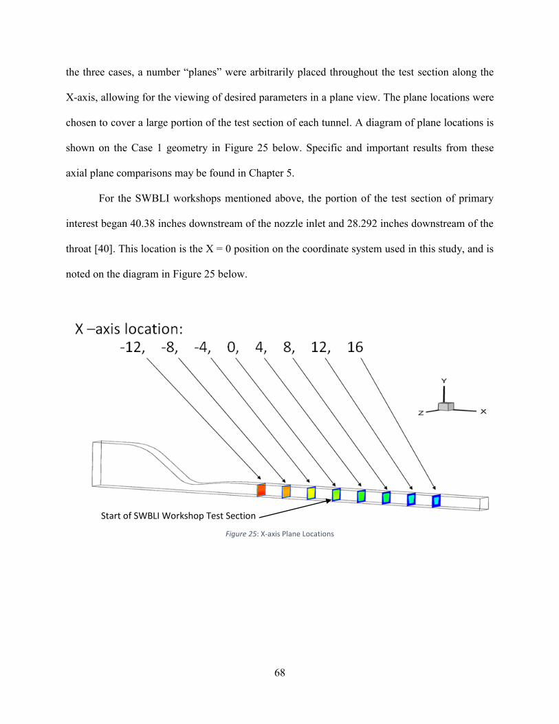
68
the three cases, a number “planes” were arbitrarily placed throughout the test section along the
X-axis, allowing for the viewing of desired parameters in a plane view. The plane locations were
chosen to cover a large portion of the test section of each tunnel. A diagram of plane locations is
shown on the Case 1 geometry in Figure 25 below. Specific and important results from these
axial plane comparisons may be found in Chapter 5.
For the SWBLI workshops mentioned above, the portion of the test section of primary
interest began 40.38 inches downstream of the nozzle inlet and 28.292 inches downstream of the
throat [40]. This location is the X = 0 position on the coordinate system used in this study, and is
noted on the diagram in Figure 25 below.
Figure 25: X-axis Plane Locations
Start of SWBLI Workshop Test Section

69
Non-Dimensional Data
It should be noted that the data output from OVERFLOW is in non-dimensional form.
OVERFLOW solves the discretized Navier Stokes equations in non-dimensional form by
making a perfect gas assumption and utilizing the appropriate speed of sound relations [35].
Flow parameters and variables are non-dimensionalized by dividing the quantity in question by a
constant reference value, usually from ambient condition, to cancel out units. A complete list of
quantities and the respective non-dimensionalized forms may be found in the OVERFLOW
User’s Manual [35]. Non-dimensional data may be used for comparison between test Cases 1, 2,
and 3 without re-dimensionalizing it because ambient/reference conditions for each case were
equal to each other. In this way, parameters between the three cases can be compared in a
straightforward fashion since the Reynolds numbers and other flow characteristics are kept
consistent.
The wind tunnel configurations under consideration in this study are driven by a vacuum,
thus the static conditions of the test facility are the total conditions found at the inlet [40], which
are listed in Table 3.
Table 3: Wind Tunnel Inlet Conditions
Total Pressure, PT 2,112 lbf/ft2
Total Temperature, TT 527 R
Mach Reference, Mref 1.8
Length Reference, Lref 1 inch
Ambient Ratio of Specific Heats, γ∞ 1.4
Specific Gas Constant, R 1,716 ft*lbf/slug*R
Following this, a further list of reference conditions may be calculated using the
isentropic relations as shown in Table 4. It should be acknowledged that the conditions found in

70
the free stream flow are typically used to initialize the flow field while reference conditions are
used in order to non-dimensionalize inputs.
Table 4: Reference Conditions
367.57
319.78 R
876.49 ft/s
1577.69 ft/s
1.688*10-7
6.698*10-4
Upon calculation of the reference conditions, OVERFLOW uses the following equation
set to non-dimensionalize the data [31]. Consequently, Equation 21 may also be used to re-
dimensionalize data.
(21)
Data Analysis
The first step in comparing the three cases was graphically displaying the variables of
interest for each X-axis plane. This enables a broad view of how the fluid behaves for each case
and allows for further inspection and identification of areas of concern. Some of this is shown
and discussed in Chapter 5.
Line plots were generated for some of the parameters following the graphical
comparison. For these plots, data was extracted from the OVERFLOW solution set at the x-axis

71
locations shown in Figure 25. The extracted data was linearly interpolated along a line from the
bottommost y-axis value to the topmost y-axis value in the center of the tunnel test section (z=0)
at each of the eight plane locations. The extracted data allowed for the magnitudes of a desired
parameter to be plotted against the y-axis, showing how specific variables change along the y-
axis at the centerline of the test sections. These line plots allow for a more exact comparison than
the planes alone. Results from the line plots and specific regions of interest (including root mean
square deviation comparisons) are shown in Chapter 5.
Another set of comparisons is made using a common CFD analysis method that can
numerically quantify differences between flow characteristics. Mass average is often computed
in terms of a parameter, such as the stagnation pressure, in order to find the weighted average
with respect to mass flow per unit area [41] in terms of a desired variable. Mass weighted flow
average is used in a similar way to represent the average momentum of the fluid at a given
position. These functions are available in Tecplot [41] and the results can be seen in Chapter 5.
The general equation to compute this mass average in terms of stagnation pressure for
compressible flow is shown below as an illustration of how flow averages are found, as
described in [42]. Mass weighted flow average is similar, but with the dot product of the flow
momentum and the surface unit normal [41] as the weighting function.
( 22)

72
Boundary Layer and Displacement Thickness
The thickness of the boundary layers present in the three tunnel configurations provides a
straightforward way to compare the test section flow. For the purposes contained in this study,
the boundary layer thickness is defined as the point at which the fluid reaches 99% of the free
stream velocity. Free stream velocity is defined as the maximum u-velocity found at each X-axis
position. A comparison between the boundary layers of each tunnel at the start of the test section
(x = 0) is found in Chapter 5.
Another important characteristic to consider when studying supersonic flows is that of the
displacement thickness, δ*. The displacement thickness is defined by White [24] as “the distance
the outer inviscid flow is pushed away from the wall by the retarded viscous layer.”
Displacement thickness is obtained from the conservation of mass through a control volume and
is a function of x only, with exact values depending on the velocity profile [24]. The equation
used is shown below, where the subscript e denotes values at the edge of the boundary layer. The
edge of the boundary layer is found using the 99% of the free stream velocity procedure
described above. For compressible flows, the displacement thickness is as shown in the equation
below. Comparisons between cases are found in Chapter 5.
(23)
Blockage
Blockage is another way to quantify how slow moving boundary layer fluid affects the
overall flow characteristics in supersonic wind tunnels. Blockage uses the displacement thickness
along each wall to calculate the area occupied by slow moving, low momentum flow that

73
“blocks” the free stream flow. Galbraith [14], et al., were able to demonstrate that blockage is of
high concern and has a large influence on determining flow field characteristics. This conclusion
was drawn from research conducted on the same University of Michigan supersonic wind tunnel
under investigation in this study. Specifically, Equation 24 shows how blockage, b, is calculated
for a given position, where Ablock denotes the area of the “blocked” flow, governed by the
displacement thickness (see Equation 23), while A denotes the overall cross sectional area of
concern. The ratio of blocked area to total cross sectional area is multiplied by 100 in order to
display blockage as a percentage of the total cross sectional area. Results from blockage
calculations are found in Chapter 5.
(24)
Specifically, the “blocked” area, Ablock, is calculated using the displacement thickness
along the boundaries of each x-axis plane location. This was done by extracting data around the
boundaries of each case (see Figure 44, Chapter 5 for specific locations) at each axial plane
location and using Equation 23 to find the displacement thickness around each of the walls for
the data points described by Figure 44. Knowing the displacement thickness for each coordinate
location makes it possible to plot the displacement thickness around the boundary walls of each
plane. From here, the cross section is divided into a series of trapezoids and rectangles, for which
the area can be calculated since the width and height of each trapezoid/rectangle is known or can
be easily calculated. An example of the area approximation scheme is shown in Figure 47 of
Chapter 5. Once all of the individual areas are calculated, the summation of all the
trapezoid/rectangle areas yields the total blockage area, Ablock, for a given plane. Equation 24 is

74
then used to find the percentage of cross section area affected by blockage. See Chapter 5 for
blockage results.
Root Mean Square Deviation
A statistical value that is often used to measure the performance of numerical models is
that of the root mean square deviation (RMSD), also known as the root mean square error [43].
This statistical parameter is useful in analyzing the differences between sets of data, often with
reference to a certain standard or accepted value. This allows for easy evaluation, not only
between the behavior of individual data sets, but also with respect to what is considered an ideal
result. The formula used to calculate RMSD [43] is shown in Equation 25, where n is equal to
the sample size and e is an error function. For the cases presented in this document, the error
function is the difference between the reference value and the results arrived at through CFD
simulation, yref -y. The reference value varies between parameters of interest depending on the
nature of the variable in question. Several RMSD comparisons are made between cases and
planes to show behavior along the test section, and are shown in Chapter 5.
(25)
For the purposes at hand, it is beneficial to display the RMSD in a percentage form to
better facilitate measures of deviation. As such, the RMSD is further divided by the applicable
reference value to arrive at a percentage value of error from the reference value. This percentage

75
method is applied where applicable but is not applied to parameters where a reference value of
zero is used.
Residuals
CFD results must be subject to some measure of quality to ensure that a valid simulation
has been carried out. Flow field simulations approach steady state when changes present in the
results become smaller from one time step to the next and begin to approach zero [44]. It is
common for CFD codes to have an auto-detect function that is able to compute when steady state
has been reached, or for the code to run for a set number of time steps and then evaluate whether
steady state has been reached after completion. [44]. Anderson [44] speaks of how residuals, so
named after the right hand sides of the continuity and momentum equations (which are not equal
to exactly zero, hence the name “residual”), are a common measure of whether a CFD solution
has converged by plotting either/or of these values against the number of time steps. Once
machine zero has been reached, simulations are said to have converged. Due to the nature of
these parameters, residual plots are shown on semi-log scales. Typically, several orders of
magnitude at the least are desired before convergence can be reached with confidence. Plots of
this nature will be utilized to illustrate that convergence has been reached in Chapter 5.

76
5. Results and Discussion
Results from the numerical study outlined in Chapter 4 are presented in this section. The
data and findings included in this chapter do not represent the full extent of work carried out, but
rather a collection of relevant displays, analyses, and findings that are particularly telling with
respect to the research goals at hand.
Convergence
Figure 26 below shows residual plots for Cases 1, 2, and 3 in order to show that the
simulations have satisfactorily converged. It can be seen that the measure of error changes
minutely by the end of the 37,000 iterations for each case. Furthermore, the residuals having
reached the order of at least 10-8
signifies that machine zero has effectively been reached and that
convergence for the iteration process has also been reached with confidence. Data analysis was
carried out with the assurance that the CFD simulations converged and that flow through each
configuration has been represented with accuracy.

77
a) Case 1
b) Case 2
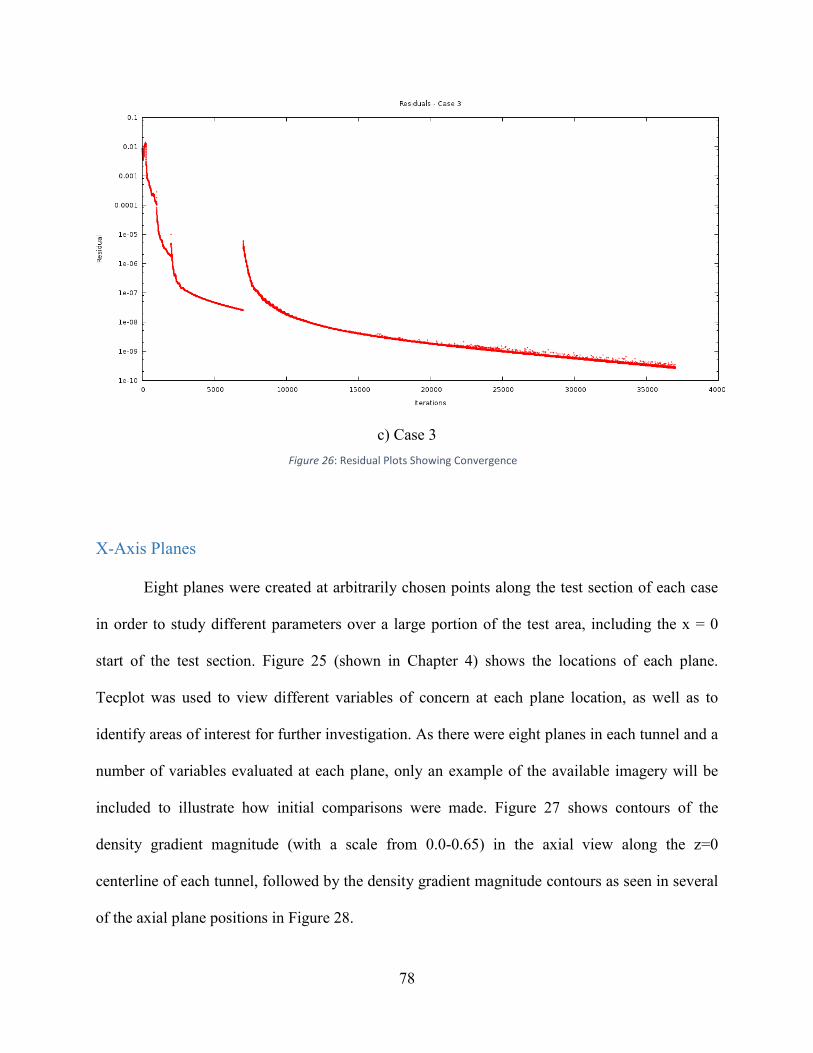
78
c) Case 3
X-Axis Planes
Eight planes were created at arbitrarily chosen points along the test section of each case
in order to study different parameters over a large portion of the test area, including the x = 0
start of the test section. Figure 25 (shown in Chapter 4) shows the locations of each plane.
Tecplot was used to view different variables of concern at each plane location, as well as to
identify areas of interest for further investigation. As there were eight planes in each tunnel and a
number of variables evaluated at each plane, only an example of the available imagery will be
included to illustrate how initial comparisons were made. Figure 27 shows contours of the
density gradient magnitude (with a scale from 0.0-0.65) in the axial view along the z=0
centerline of each tunnel, followed by the density gradient magnitude contours as seen in several
of the axial plane positions in Figure 28.
Figure 26: Residual Plots Showing Convergence
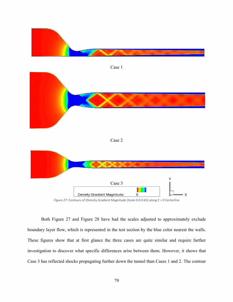
79
Case 1
Case 2
Case 3
Figure 27: Contours of (Density Gradient Magnitude (Scale 0.0-0.65) along Z = 0 Centerline
Both Figure 27 and Figure 28 have had the scales adjusted to approximately exclude
boundary layer flow, which is represented in the test section by the blue color nearest the walls.
These figures show that at first glance the three cases are quite similar and require further
investigation to discover what specific differences arise between them. However, it shows that
Case 3 has reflected shocks propagating further down the tunnel than Cases 1 and 2. The contour
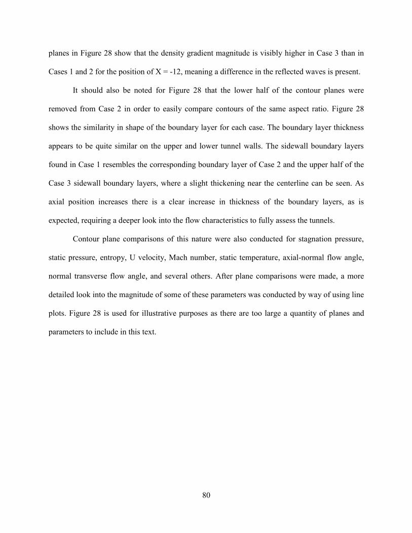
80
planes in Figure 28 show that the density gradient magnitude is visibly higher in Case 3 than in
Cases 1 and 2 for the position of X = -12, meaning a difference in the reflected waves is present.
It should also be noted for Figure 28 that the lower half of the contour planes were
removed from Case 2 in order to easily compare contours of the same aspect ratio. Figure 28
shows the similarity in shape of the boundary layer for each case. The boundary layer thickness
appears to be quite similar on the upper and lower tunnel walls. The sidewall boundary layers
found in Case 1 resembles the corresponding boundary layer of Case 2 and the upper half of the
Case 3 sidewall boundary layers, where a slight thickening near the centerline can be seen. As
axial position increases there is a clear increase in thickness of the boundary layers, as is
expected, requiring a deeper look into the flow characteristics to fully assess the tunnels.
Contour plane comparisons of this nature were also conducted for stagnation pressure,
static pressure, entropy, U velocity, Mach number, static temperature, axial-normal flow angle,
normal transverse flow angle, and several others. After plane comparisons were made, a more
detailed look into the magnitude of some of these parameters was conducted by way of using line
plots. Figure 28 is used for illustrative purposes as there are too large a quantity of planes and
parameters to include in this text.
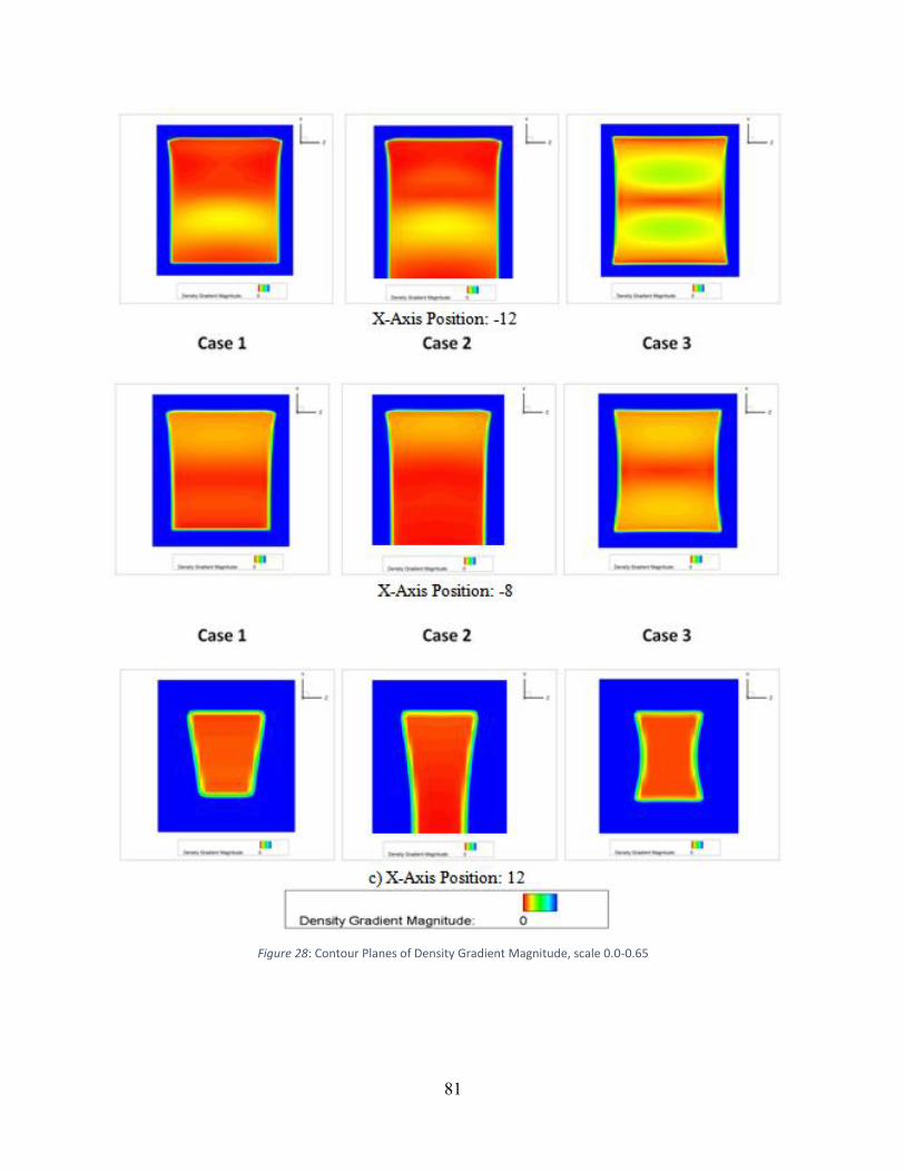
81
Figure 28: Contour Planes of Density Gradient Magnitude, scale 0.0-0.65

82
Line Plot Comparisons
Line plot comparisons enable a more direct inspection of the magnitude of variables in
question. Plots were generated that portray parameters magnitudes at each of the eight axial
stations along the z=0 centerline plotted against the y-axis position. This allows for the variation
of each variable in the y direction to be shown along the centerline of each tunnel.
Axial Normal Flow Angle
Line plot comparisons of axial-normal flow angle show a discrepancy between the three
cases. Figure 29 shows axial-normal flow angle of each axial station plotted together against the
y-axis. An axial-normal flow angle of 0º in the x-y plane is desired for an ideal test section.
Deviation from 0º may cause flow conditions to contribute to errors in test results. The lowest
deviation from 0º is desired since ideal flow conditions are rarely achievable in a practical
setting.

83
a) Case 1 b) Case 2
c) Case 3
Figure 29: Axial Normal Flow Angle Line Plots (degrees) for All Axial Stations
Figure 29a and Figure 29b show that Cases 1 and 2 have flow angle changes of similar
magnitude, both peaking at nearly 0.6º, while Figure 29c shows that Case 3 has a peak axial-
normal flow angle of close to 0.2º, roughly one third that of Cases 1 and 2. The root mean square
deviation (RMSD) of the axial-normal flow angle was calculated at each axial station to further
illustrate how flow behaves for each case throughout the test section. The results of the root

84
mean square deviation calculations are shown graphically in Figure 30 with a table of results
available in Table 7 of Appendix A. It should be noted that the reference value used was 0º and
that calculations include the whole cross section of the tunnel at each axial station (not just along
the z=0 centerline).
Figure 30: Axial-Normal Flow Angle Root Mean Square Deviation
Figure 30 and Table 7 corroborate what is seen in Figure 29; Cases 1 and 2 behave
similarly, with Case 3 having the most consistent flow that is the least deviated from 0º. Cases 1
and 2 both have higher deviations from ideal flow as well as less consistency throughout the
axial stations. All three cases generally trend toward a decrease in deviation as flow travels down
the tunnel, however, Cases 1 and 2 are not as consistent as Case 3, which has a relatively steady

85
amount of deviation throughout the length of the tunnel. The consistently low deviation found in
Case 3 shows that this configuration is the best in terms of axial-normal flow angle.
Axial Transverse Flow Angle
Similar to the axial normal flow angle, line plot comparisons of the axial transverse (x-z
plane) flow angle show that there are indeed differences in flow angle between the three tunnel
cases. Figure 31c shows that Case 3 has much less angle variation in the axial-transverse
direction, with its values appearing to be virtually equal to zero for all axial stations (all
appearing as a single vertical line in the figure). Figure 31a and Figure 31b show that a much
greater degree of angle variation exists in Cases 1 and 2, with a particularly noticeable
occurrence of angle change in Case 2. However, if the outlying large angle is excluded from
Case 2, it can be seen that Cases 1 and 2 are close to one another. The fact that Cases 1 and 2 are
similar does not necessarily prove that a symmetric configuration is always better; rather the
symmetric and equal aspect ratio configuration of Case 3 is by far the best configuration with
respect to axial transverse flow angle, as shown by the virtually non-existent changes in angle
throughout the test section.
Once again, the RMSD is calculated across the entirety of each of the eight axial planes
in order to show the total amount of deviation from an expected value. Again, a reference value
of 0º is used and signifies the desire to have uniform, parallel flow in the test section. Results are
shown graphically with the same scale in Figure 32 with the corresponding values tabulated in
Table 8 in Appendix A. The trends in the RMSD data verify that the centerline trends of Figure
31 also appear across each axial station in all x-axis positions. That is, Cases 1 and 2 have similar
trends, but a much greater magnitude of deviation is present when compared to Case 3. Cases 1
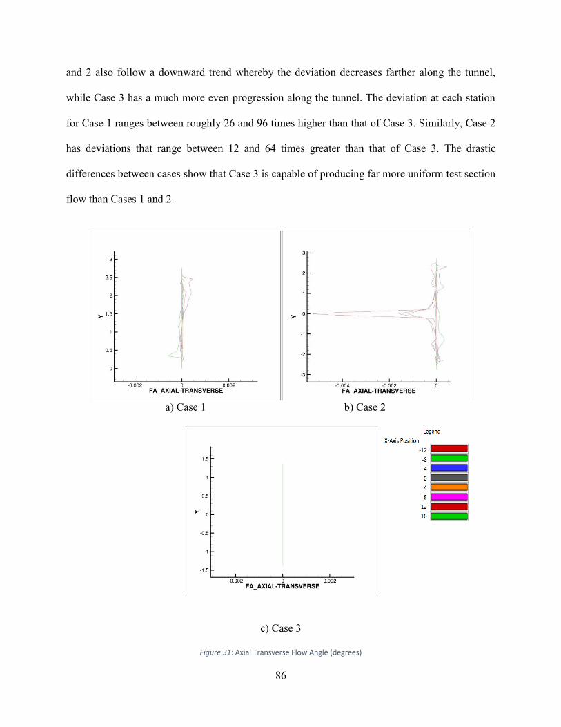
86
and 2 also follow a downward trend whereby the deviation decreases farther along the tunnel,
while Case 3 has a much more even progression along the tunnel. The deviation at each station
for Case 1 ranges between roughly 26 and 96 times higher than that of Case 3. Similarly, Case 2
has deviations that range between 12 and 64 times greater than that of Case 3. The drastic
differences between cases show that Case 3 is capable of producing far more uniform test section
flow than Cases 1 and 2.
a) Case 1 b) Case 2
c) Case 3
Figure 31: Axial Transverse Flow Angle (degrees)
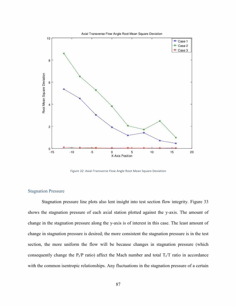
87
Figure 32: Axial-Transverse Flow Angle Root Mean Square Deviation
Stagnation Pressure
Stagnation pressure line plots also lent insight into test section flow integrity. Figure 33
shows the stagnation pressure of each axial station plotted against the y-axis. The amount of
change in the stagnation pressure along the y-axis is of interest in this case. The least amount of
change in stagnation pressure is desired; the more consistent the stagnation pressure is in the test
section, the more uniform the flow will be because changes in stagnation pressure (which
consequently change the Pt/P ratio) affect the Mach number and total Tt/T ratio in accordance
with the common isentropic relationships. Any fluctuations in the stagnation pressure of a certain

88
location will result in a corresponding change in the Mach number or temperature ratio at that
same location. Fluctuations of this manner are not conducive to producing uniform test section
flow characteristics. Figure 33 shows that Cases 1, 2, and 3 have stagnation pressures of similar
magnitudes, but that Case 3 fluctuates the least with respect to the y axis. Case 1 has a more
pronounced increase in stagnation pressure as flow approaches the upper wall of the tunnel than
Case 3. Case 2, however, has a higher and more dramatic increases at both the upper and lower
tunnel walls, as well as an increase near the center of the tunnel. Case 3 is visibly the most
consistent with respect to y and has the least amount of variation in near the upper and lower
boundaries.
It should be noted that since Case 2 has twice the cross sectional area as that of Cases 1
and 3 and thus has double the core flow. When comparing the three cases, it must be realized that
this is expected behavior; Case 2 has the greatest area across which stagnation pressure may
affect the flow, but having more area does not necessarily mean better results. Consistency of the
stagnation pressure across the area present in each case is the most telling factor about stagnation
pressure.
Once again, the RMSD of the stagnation pressures was calculated to help quantify the
differences in flow characteristics. Tabulated results are shown in Table 9 in Appendix A and
graphically in Figure 34 in percent form. The reference value used for calculating the root mean
square deviation was the mass weighted average of the stagnation pressure at each axial station
for each case. This value was chosen for several reasons. First, it is desired to have a high
stagnation pressure, which denotes little fluctuation of this value between planes. However,
simply using a reference value of the maximum stagnation pressure at each station would be
skewed by the slow moving boundary layer fluid. Similarly, taking an average of the stagnation

89
pressure would also be affected by the boundary layer flow. Boundary layer flow should not
affect the reference value since the core flow through the test section is “more important” in
terms of practical use. As such, using the mass weighted average of stagnation pressure provides
the best measure of the conditions found at each plane by weighting the core flow. This places
more value on the core flow, allowing for a reference value to be used that reflects mostly
reflects core flow behavior. Again, the RMSD is calculated over the entirety of each axial plane.
Figure 34 shows that Cases 1 and 3 behave similarly, but that Case 3 has the least deviation from
the desired stagnation pressure at each axial station, which helps to solidify what is seen visually
in Figure 33. Case 2 has the least deviation before the test section, but also the most erratic
transitions between planes. Furthermore, once the test section begins, Case 2 performs less
desirably than Case 1 and 3. Case 3 has overall best stagnation pressure profiles when
considering both consistency and magnitude of deviation.

90
a) Case 1 b) case 2
c) Case 3
Figure 33: Stagnation Pressure Line Plots for all Axial Stations

91
Figure 34: Stagnation Pressure Root Mean Square Deviation
Static Pressure
A similar analysis is carried out for the static pressure. Line plots are generated for each
case along the Z = 0 centerline and plotted against the Y axis position. Figure 35 shows that Case
3 has generally the least variation in pressure along the Y axis, with the exception of the first two
axial stations (x = -12 and x = -8). Indeed, this is corroborated in Figure 36, which displays the
RMSD data for each entire x-axis plane, using a reference value of the maximum static pressure
found at each axial location and displayed in percentage form. Perhaps the most interesting
feature of Figure 36 is the dramatic decrease in the amount of deviation present in Case 3; by the

92
start of the x = 0 station, the start of the test section [40], the deviation in static pressure is
practically zero, while Cases 1 and 2 are much higher and have less consistency throughout the
remaining portion of the test section, showing that Case 3 has the best static pressure conditions
the given configurations. Tabulated RMSD data is found in Table 10 of Appendix A.
a) Case 1 b) Case 2
c) Case 3
Figure 35: Static Pressure Line Plots for All Axial Stations a) Case 1, b) Case 2, c) Case 3

93
Figure 36: Static Pressure Root Mean Square Deviation
Entropy
The line plots for each the entropy of each case along the z = 0 centerline versus the y-
axis are shown in Figure 37. At a glance, it is difficult to discern significant differences between
the cases. Figure 38 depicts the RMSD data for each axial plane, using a reference value of zero.
Table 11 of Appendix A has a full list of RMSD results. Case 3 generally has less deviation than
that of Cases 1 and 2, following the trend observed in earlier pressure and flow angle data. The
combination of lower deviation and a strong level of consistency makes Case 3 the clear leader
in terms of entropy behavior.

94
a) Case 1 b) Case 2
c) Case 3
Figure 37: Entropy Line Plots for All Axial Stations

95
Figure 38: Entropy Root Mean Square Deviation
Mach Number
A primary concern of flow through a wind tunnel is not only uniformity in terms of flow
direction, steadiness, and pressure characteristics, but also the consistency of flow Mach
numbers along the tunnel. The Mach number is examined to detail any differences between the
three cases. Figure 39 shows line plot comparisons along the z = 0 centerline of Mach number
plotted versus the y axis. Much like other parameter discussed above, it is desired to have little
variation present in the Mach number so as to have a configuration with flow as consistent as
possible. As such, the line plots are able to show that Cases 1 and 2 have more variation in the
Mach number with respect to y than Case 3. Particularly noteworthy is how much more uniform
96
the data appears to be for Case 3 at the start of and throughout the test section; the line plots
appear to be virtually straight up and down (signifying little change with y), while Cases 1 and 2
are visibly less uniform, as seen by the more sloped lines present on the plots.
The root mean square deviation is again calculated to show the behavior of Mach number
over the entirety of each plane. The way in which the reference value is computed must be
addressed in order to examine the RMSD of the Mach number. Since the systems being studied
contain viscous flow, boundary layer effects continually work to slow the free stream flow, thus
using a simple reference value of Mach 1.8, the nominal operating condition, is not possible.
Doing so would result in disproportionately high levels of deviation as flow travels downstream
due to the inherent slowing of the flow. Rather, a more local reference value must be used for
each axial plane in question. A local reference Mach will ensure an accurate measure of variation
across planes with respect to the overall conditions experienced at the location in question.
Simply calculating the average and/or weighted average of Mach number at each station for each
tunnel is not sufficient either, because any averages will be skewed by the slow moving
boundary layer effects. Examining the y position of the curved, slow moving fluid and the way
these lines converge to zero in the line plots of Figure 39 should make this apparent. A method to
remove some of the boundary layer effects must be utilized to fully analyze the variation of the
test section core flow with respect to Mach number.
The displacement thickness is taken advantage of in order to accomplish this.
Displacement thickness is calculated for the x = 0, 4, 8, 12, and 16 location planes. This process
is discussed in detail toward the end of this Chapter in its own section. After calculating the
displacement thickness of each wall at each x location, it is possible to create new planes that are
bounded by the coordinates of the calculated displacement thicknesses. These new planes

97
exclude the fluid moving through the displacement thickness region and are thus free of some of
the influence of the slow moving fluid found therein. The new planes are much more
representative of the true behavior of flow through the test section core. Next, the average Mach
numbers of the new “displacement thickness free” planes are calculated for each tunnel and x
location and are used as the reference values in the corresponding RMSD calculations. Figure 40
shows the RMSD results in percent form, which are also tabulated in Table 12 of Appendix A.
Figure 40 shows similar results to Figure 39, that is, Case 3 seems to be the best
candidate for creating the most uniform flow in terms of Mach number. Case 3 experiences less
deviation than Case 1 for the first three locations of the test section. Case 1 has less deviation for
the last two locations. However, it must be acknowledged that in a practical application any test
geometry will likely be placed nearer the beginning of the test section than toward the end,
reflecting the superiority of Case 3. Once again, too, Case 3 is more consistent between plane
locations; the progression of Case 3 appears nearly linear from start to finish whereas Case 1 is
much more curved, especially at the start of the test section. It should be noted that Case 2 has
the least amount of deviation overall, however this must not be taken at face value; Case 2 is
inherently less affected by displacement thickness effects since it has twice the cross sectional
area as that of Cases 1 and 3. The comparable displacement thickness values found on all three
cases mean that as a ratio of slow moving to fast moving fluid, Case 2 will be overall the least
affected by slow moving flows due to its larger area. However, in terms of consistency and low
amount of deviation in practical test section locations, Case 3 is the most opportune
configuration.
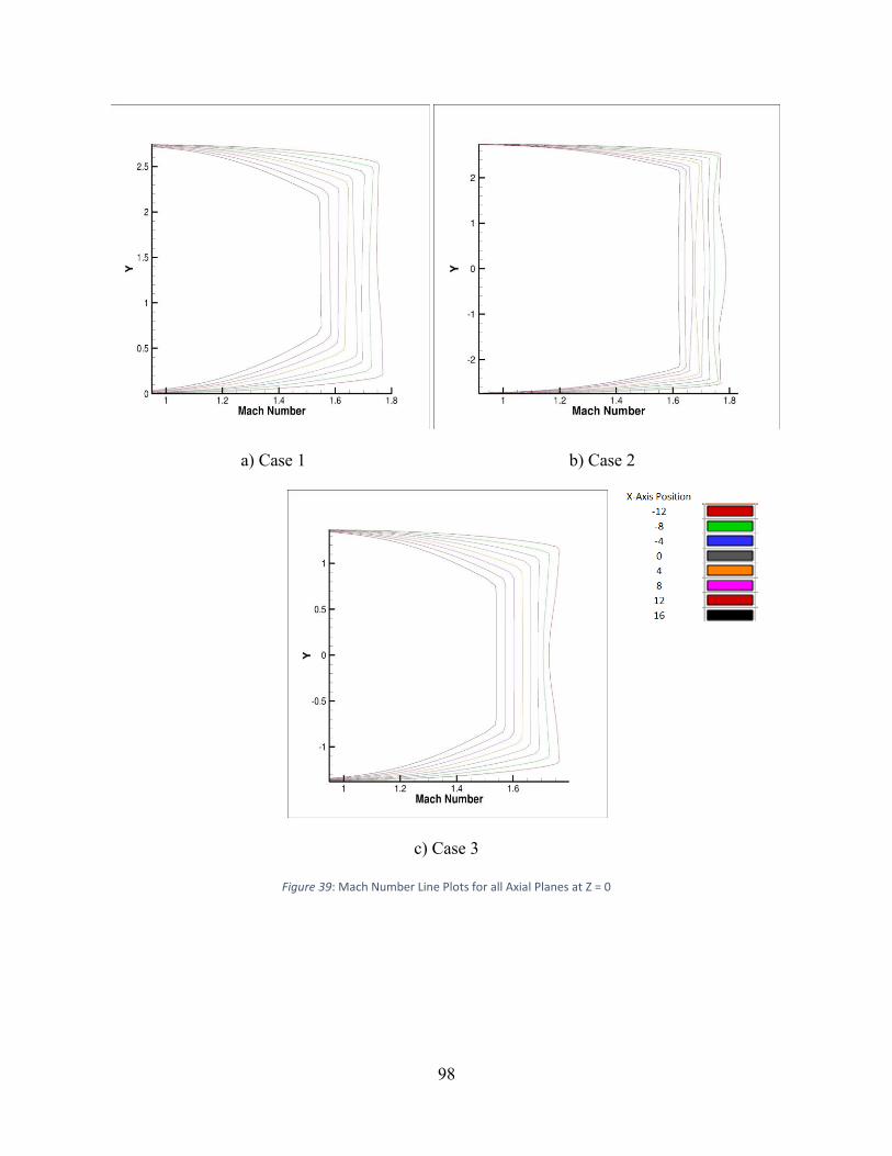
98
a) Case 1 b) Case 2
c) Case 3
Figure 39: Mach Number Line Plots for all Axial Planes at Z = 0
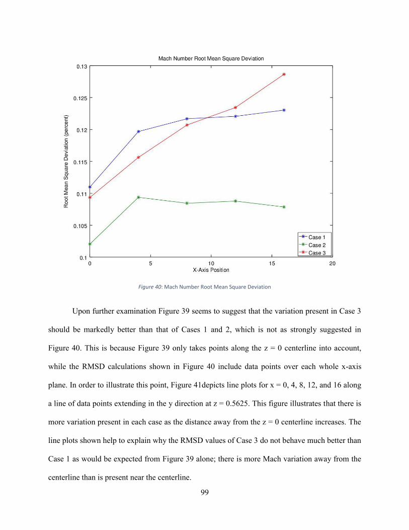
99
Figure 40: Mach Number Root Mean Square Deviation
Upon further examination Figure 39 seems to suggest that the variation present in Case 3
should be markedly better than that of Cases 1 and 2, which is not as strongly suggested in
Figure 40. This is because Figure 39 only takes points along the z = 0 centerline into account,
while the RMSD calculations shown in Figure 40 include data points over each whole x-axis
plane. In order to illustrate this point, Figure 41depicts line plots for x = 0, 4, 8, 12, and 16 along
a line of data points extending in the y direction at z = 0.5625. This figure illustrates that there is
more variation present in each case as the distance away from the z = 0 centerline increases. The
line plots shown help to explain why the RMSD values of Case 3 do not behave much better than
Case 1 as would be expected from Figure 39 alone; there is more Mach variation away from the
centerline than is present near the centerline.

100
Regardless, the overall variation over each plane and the behavior of Mach number
through the test section remains the best in Case 3. The overall planes experience smoother
transitions between planes and lower values for the first three test section planes (arguably the
most important portion of the test section). Both low variation in value and between planes is
desired, making Case 3 the most suited to producing flow with desirable Mach characteristics.
a) Case 1 b) Case 2
c) Case 3
Figure 41Mach Number Line Plots for X = 0, 4, 8, 12, and 16 Planes at Z = 0.5625

101
Averages
The mass weighted average is often used as a measure of mass flow per unit area of a
certain variable. Since a higher mass average with respect to stagnation pressure means flow has
been less affected by boundary layers, relatively speaking, the mass weighted average with
respect to stagnation pressure is able to shows which tunnel has the best core flow
characteristics. Higher stagnation pressure mass average indicates test section flow that is the
most ideal. Figure 42 shows the mass weighted average of stagnation pressures at each axial
station with tabulated data found in Table 13 of Appendix A. Similarly, mass weighted flow
average is another way to inspect the core flow. This parameter is a measure of flow momentum
per unit area, rather than a measure of mass flow per unit area. A higher momentum per unit area
is desired because higher momentum fluid means it has been affected less by boundary layer
effects, relatively speaking. Figure 43 below shows the comparison between cases and axial
stations for stagnation pressure with tabulated results in Table 14 of Appendix A.

102
Figure 42: Stagnation Pressure Mass Weighted Average

103
Figure 43: Stagnation Pressure Mass Weighted Flow Average
Figure 42 and Figure 43 show that the highest mass flow and momentum occurs in Case
2, which is due to the increased height of this configuration. Increasing the area by a factor of
two means an increase in the aspect ratio, which corresponds to an increase in the weighted area
and mass and flow averages for this case. Cases 1 and 3 are very similar to one another, with
Case 3 being overall slightly higher than that of Case 1. To numerically illustrate the differences
between the mass weighted and mass weighted flow averages, the percent change with respect to
Case 1 at each axial station for Cases 2 and 3 is shown in Table 5 and Table 6. Case 2 has the
highest percent change with respect to Case 1, ranging from 1.83 to 5.59% for the mass weighted
average and between 1.51 to 4.76% for the mass weighted flow average. Again, this is expected

104
because of the larger aspect ratio found in Case 2. Case 3 is much closer to Case 1, with percent
changes of mass weighted average ranging from 0.087 to 0.16% and -0.092 to 0.13% for the
mass weighted flow average. It is also observed, that Case 2 has a higher percent change for both
sets of averages as the axial station increases, whereas Case 3’s percent change with respect to
Case 1 decreases as the axial station increases.
Table 5: Percent Change of Stagnation Pressure Mass Weighted Average wrt. Case 1
Percent Change of Stag. P Mass
Weighted Avg. wrt. Case 1
X-Axis Position Case 2 Case 3
-12 1.827047 0.164438
-8 2.477956 0.162122
-4 3.07839 0.145103
0 3.632861 0.119468
4 4.205675 0.121282
8 4.66694 0.110622
12 5.14292 0.092816
16 5.590367 0.087394
Table 6: Percent Change of Stagnation Pressure Mass Weighted Flow Average wrt. Case 1
Percent Change of Stag. P Mass
Weighted Flow Avg. wrt. Case 1
X-Axis Position Case 2 Case 3
-12 1.509508 0.131790
-8 2.060336 0.117218
-4 2.578836 0.089802
0 3.075851 0.058572
4 3.539613 0.025175
8 3.976469 -0.011243
12 4.384943 -0.051158
16 4.763869 -0.092347

105
Boundary Layer Thickness
A study of test section core flow characteristics would not be complete without
considering boundary layer thicknesses. For the purposes herein, the boundary layer thickness is
defined as the point at which the fluid reaches 99% of the free stream velocity. Free stream
velocity is defined as the maximum u-velocity at each of the eight x-axis planes. The boundary
layer of each tunnel configuration was computed in this manner at the start of the test section, x
= 0, for three equally spaced z-axis locations, and seven equally spaced y-axis points are placed
in equivalent locations for each case. This allows for a boundary layer profile of each case to be
displayed at the start of the test section. It should be noted that an extra calculation point was
added to Case 2 in order to keep the same computational resolution as Cases 1 and 3 (necessary
because of the doubled height of Case 2). A complete diagram of each of the points at which the
boundary layers have been calculated can be found in Figure 44. The thickness of boundary
layers is desired to be as small as possible.

106
Figure 44: Diagram of Boundary Layer Calculation Points
107
With calculations complete for the upper, lower, and sidewall boundary layers, it is
possible to plot the boundary layer contours of each case on a single cross section of the tunnel in
order to compare behavior at the x = 0 starting location of the test section. This comparison is
seen in Figure 45. It should be noted that in order to do this, only the upper half of Case 2 was
plotted in order to compare the three cases on an equal aspect ratio. A complete table of
computed boundary layer thicknesses may be found in Table 15 of Appendix A. Figure 45 Show
that Cases 1 and 2 are quite similar, as expected, due to the symmetry found over the x-axis.
However, due to the doubled height of Case 2, there is no lower boundary layer present in this
comparison. All three cases have an upper boundary layer that is essentially equal; it is the
sidewalls and lower plane where differences arise. Cases 1 and 2 experience thickening of the
sidewall boundary layesr in the low y-axis region, which is similar to the thickening found in the
middle range of y-axis values of Case 3, meaning the differences between cases in the sidewall
regions is not a primary concern. Perhaps the most interesting comparison is that of the lower
boundaries of Cases 1 and 3. Case 1 has a noticeably thicker lower boundary layer as compared
to Case 3, lending to the conclusion that Case 3 is more conducive to producing optimal flow
conditions than Cases 1 and 2. In order to further quantify the differences in boundary layers, the
displacement thickness was investigated.

108
Figure 45: Boundary Layer Comparison
.
Displacement Thickness
The displacement thickness, described in Chapter 4, is an important characteristic that
describes how much a nozzle profile must be adjusted in order to achieve the desired mass flow
characteristics to have effectively inviscid flow conditions. Small displacement thicknesses are
desired in order to minimize the amount of compensation that must occur in order to achieve
inviscid core flow. The displacement thickness of the lower boundary was calculated at the z = 0
centerline on each of the eight axial planes to compare this value between cases. Figure 46 shows
the results, with tabulated results in Table 16 of Appendix A.
Figure 46 shows that the displacement thickness of each tunnel configuration increase
with axial position, an expected occurrence. While the magnitudes do not differ drastically

109
between cases, there are differences between the three. Both Cases 1 and 2 are less consistent
than that of Case 3; Cases 1 and 2 experience increases in the displacement thickness in a more
erratic way, increasing by differing amounts between each plane. Case 3, conversely, has
smoother transitions between planes and behaves in a more predictable fashion. It should be
noted that although overall magnitudes between the cases are similar, Case 1 has noticeably
larger displacement thicknesses at all locations downstream of the start of the test section, a
feature which is decidedly detrimental to performance. Case 3 is the best configuration in terms
of displacement thickness since both consistency and small size of displacement thickness are
desired; Case 3 exhibits both the smoothest transitions travelling downstream and markedly
lower displacement thicknesses throughout the test section than that of Cases 1.

110
Figure 46: Lower Wall Displacement Thickness at Z = 0 (inches)
The behavior of displacement thickness is a significant area of concern since it is this
parameter that governs the amount of adjustment required in order to consider core flow as
inviscid. As discussed in Chapter 1, Case 2 (the UM tunnel) is unable to account for
displacement thickness effects found on the lower wall. This means that the displacement
thickness acts as an effective boundary, increasing in thickness in the x direction, and preventing
the flow from being turned back to parallel and helping to create non-uniform flow. Cases 2 and
3 do not have this issue and thus are inherently better suited at creating test section flow that is
more uniform. This is made abundantly clear by the calculations shown in Figure 46.

111
Blockage
Blockage may be used as a measure of how much of the cross sectional area of the tunnel
is affected by slower moving flow, as governed by displacement thickness. As discussed in
Chapter 4, Galbraith [14] et al. showed that blockage plays an important part in determining flow
characteristics for the specific UM tunnel under investigation here. Since blockage is detrimental
to such things as the mass flow rate characteristics of the nozzles, it is desired to have as little
blockage as possible. As such, the displacement thickness was used to calculate the blockage
area for the three test cases. This was done by extracting data in the same locations shown in
Figure 44 at each axial plane. Then, the displacement thickness is calculated at each of the data
points described by Figure 44 for each axial position. Knowing the displacement thickness for
each coordinate location makes it possible to plot the displacement thickness (see Equation 23,
Chapter 4) around the boundary walls of each plane. From here, the cross section is divided into
a series of trapezoids and rectangles, for which the area can be calculated since the width and
height of each trapezoid/rectangle is known or can be easily calculated. An example of the area
approximation scheme is shown in Figure 47, which happens to be for Case 3 at x = 12. Once all
of the individual areas are calculated, the summation of all the trapezoid/rectangle areas yields
the total blockage area for a given plane, Ablock. Equation 24 (see Chapter 4) is then used to find
the percentage of cross section area affected by blockage. This process was carried out for each
case, beginning with the start of the test section.
Figure 48 depicts the blockage area in square inches found on each plane beginning at x =
0. Upon examination, this figure shows that Case 3 has the smallest amount of blockage area
present at each x plane. Cases 1 and 2 both behave similarly and begin the test section with
blockage amounts similar to that of Case 3. However, as the test section progresses, Cases 1 and

112
2 both experience an increase in blockage at a quicker rate than Case 3; all three cases begin
similarly, but Cases 1 and 2 end the test section with roughly 0.2 in2 more blockage present than
in Case 3. Figure 49 depicts the percent of the area present for each case that is comprised of
blockage. It is important to note, that since Case 2 has twice the cross sectional area compared to
Cases 1 and 3 that the percentage of blocked flow will be correspondingly less than that of Case
1 and 3. It is clear when looking at Figure 49 that Case 1 has the highest percentage of blockage.
Case 3 both has less blockage present and has a more gradual increase in the amount of blockage
as position increases. At the end of the test section Case 3 experiences blockage levels roughly
3.5% less than that of Case 1. Clearly, in terms of consistency and the desired low levels of this
parameter, Case 3 is the best choice and should produce flow with blockage levels the least
likely to detrimentally affect the overall flow field. Tabulated blockage data may be found in
Appendix A, Table 17.
Figure 47: Example of Blockage Area Approximation Scheme (Case 3 at x = 12)

113
Figure 48: Blockage Area Downstream of Test Section (in2)
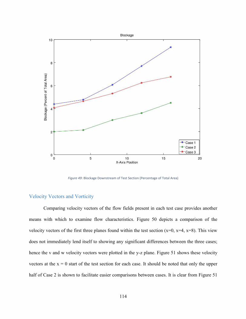
114
Figure 49: Blockage Downstream of Test Section (Percentage of Total Area)
Velocity Vectors and Vorticity
Comparing velocity vectors of the flow fields present in each test case provides another
means with which to examine flow characteristics. Figure 50 depicts a comparison of the
velocity vectors of the first three planes found within the test section (x=0, x=4, x=8). This view
does not immediately lend itself to showing any significant differences between the three cases;
hence the v and w velocity vectors were plotted in the y-z plane. Figure 51 shows these velocity
vectors at the x = 0 start of the test section for each case. It should be noted that only the upper
half of Case 2 is shown to facilitate easier comparisons between cases. It is clear from Figure 51
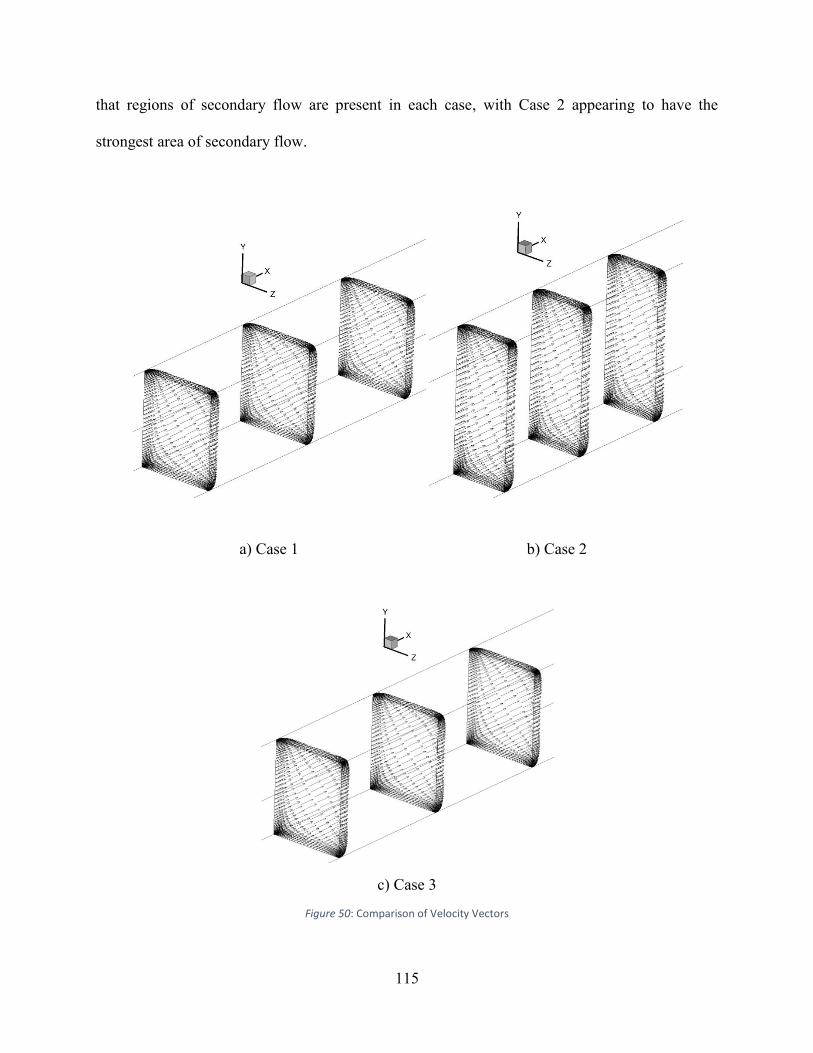
115
that regions of secondary flow are present in each case, with Case 2 appearing to have the
strongest area of secondary flow.
a) Case 1 b) Case 2
c) Case 3
Figure 50: Comparison of Velocity Vectors

116
a) Case 1 b) Case 2
c) Case 3
Figure 51: V and W Velocity Vectors at x = 0

117
Streamlines were seeded into the test section of each case at corresponding locations to
allow for better visualization of the secondary flow, shown in Figure 52.
a) Case 1 b) Case 2
c) Case 3
Figure 52: Secondary Flow Streamlines

118
Several more v-w velocity vector streamline views are found in Appendix B. Case 2
appears to have secondary flow areas that are the largest. Conversely, Case 3 has the smallest
secondary flow regions. However, Case 3 has 4 secondary flow zones, while Cases 2 and 1 only
have two. Again, while it is clear that secondary flow exists, it is difficult to quantify at this
point, so Figure 53 was generated to further show where differences are present.
This figure shows axial streamlines seeded in corresponding locations for each test case
that are placed such that the streamlines pass through the centers of the secondary flow zones
shown in Figure 52. Since the u velocity components are of much greater magnitude than the v
and w components, there are only small perturbations visible in the axial direction. Figure 53a
shows encircled regions of perturbations that are magnified in Figure 53b, which shows that
Case 3 experiences flow less deviated from the axial direction as compared to Cases 1 and 2,
which have clearly visible ripples present in the streamlines. At this point, from the standpoint of
visual perturbations alone, it can be seen that Case 3 has the least amount of deviation from the
axial direction, leading to the conclusion that the secondary flows within Case 3 are likely to be
smaller than those found in Cases 1 and 2, making Case 3 the better choice of the three.
However, to truly quantify the differences between the three cases, vorticity was taken into
consideration.
Vorticity is not a desired aspect of high speed flow, but applications such as wind tunnels
experience it nonetheless. Thus, it is desired to have as small values of vorticity as possible. The
root mean square deviation of the x-axis vorticity of each tunnel is shown in Figure 54, where a
reference value of zero was used. This corroborates the findings from Figure 53 that Case 3 has
core flow of the highest integrity. Figure 54 shows that Cases 1 and 2 behave similarly, but are
erratic as flow moves downstream, with differing amounts of change between each axial plane.

119
Case 3, conversely, experiences flow that has an overall deviation away from zero much less
than that of Cases 1 and 2, with values of deviation often less than half of Cases 1 and 2. An
important aspect to note, much like previous parameters that have been studied, is the greater
level of consistency found in Case 3; not only is the amount of axial vorticity present in Case 3
less than Cases 1 and 2, but the variation between axial planes is subject to less change as well.
Both Figure 53 and Figure 54 show that the influence of secondary flows and vorticity
present are markedly less pronounced in Case 3, showing once again that Case 3 is the
configuration that is most conducive to producing uniform flow in the test section.

120
Case 1 Case 2 Case 3
a) Axial Streamlines
Case 1 Case 2 Case 3
b) Magnified Streamline Perturbations
Figure 53: Axial Streamline Comparison

121
Figure 54: Root Mean Square Deviation of Axial Vorticity

122
6. Conclusions and Recommendations
Summary and Conclusions
A Reynolds averaged Navier Stokes CFD study has been carried out in order to
determine whether asymmetric supersonic wind tunnels have flow characteristics that are equally
reliable for use in producing uniform test section flow for application in supersonic testing.
Important characteristics that determine the integrity of flow through test sections include but are
not limited to the stagnation pressure, static pressure, flow angles, mass/momentum averages,
and vorticity.
An asymmetric supersonic wind tunnel configuration, Case 1, (corresponding to an
existing test facility housed at the University of Michigan) was used to create two symmetrically
equivalent configurations with which to make comparisons. Cases 2 was an “inviscid” and fully
symmetric reflection of Case 1 with the lower wall (the new centerline) removed and double the
cross sectional area of Case 1. Case 3 was a reflection of Case 1, again with the lower wall
removed, that was scaled such that Cases 1 and 3 had equal cross sectional area.
The insight gleaned from the CFD study presented shows that Case 3, the equal area
symmetric reflection, yields test section flow that is reasonably the most consistent and uniform
of the three cases. None of the cases are perfect; boundary layer effects take a toll on all three,
but the most consistent data comes from Case 3. The deviation from desired values for axial-
normal flow angle, axial-transverse flow angle, stagnation pressure, static pressure, entropy, and
vorticity show that Case 3 experiences the least amount of deviation from uniform flow.
Furthermore, Case 3 is subject to the least amount of displacement thickness, an important flow
characteristic that must be accounted for in the design phase. Moreover, streamlines and velocity
vector profiles show that Case 3 has the smallest secondary flow zones present in the test section.
123
While there may not be significant differences in terms of mass and momentum average,
however, it is important to consider all characteristics together as a system since no single
parameter is a deciding factor in the overall soundness of test section flow and to focus on what
major differences were shown.
Recommendations
Sufficient evidence has been provided to show that asymmetric nozzles do not produce as
uniform flow as an equivalent aspect ratio symmetric configuration. Further simulations could be
carried out which strive to determine whether accounting for the displacement thickness on the
lower plane will yield more desirable test section flow. It is easy enough to point out that Case 3
has less displacement thickness than that of the asymmetrical Case 1. However, the true
implication of this statement goes further; since Case 1 was designed to have a lower wall that is
parallel to the test section centerline, it is impossible to account for the displacement thickness.
This means that the flow will perpetually be turned slightly away from parallel as waves interact
with the inclined effective wall induced by the displacement thickness. Since displacement
thickness increases axially, this problem will on get worse throughout the test section. Further
simulations could correct the lower plane to account for this issue and study the resulting effects
of a newly created asymmetric supersonic nozzle that has both upper and lower contours that
take displacement thickness into account.
Another factor that helps Case 3 achieve more uniform flow is the more gradual
expansion section it has as compared to Cases 1 and 2. Since Case 3 has two contours with
which to expand flow, each respective wall expands more gradually than the more rapid single
expanding wall found in Case 1 (and its reflection in Case 2). This effect could further be studied

124
by generating another nozzle contour, whereby all four wall boundaries are contoured to help
expand the flow. This would further decrease amount of expansion present on each wall and
possibly increase the level of flow uniformity even further.

125
7. Bibliography
1. Crowe, C. T., Elger, D. F., Williams, B. C., Roberson, J. A., Engineering Fluid
Mechanics, John Wiley and Sons Inc., Ninth Edition, Hoboken, New Jersey, 2009.
2. Babinsky, H., Harvey, J. K., Shock Wave-Boundary Layer Interactions, Cambridge
University Press, Cambridge, United Kingdom, 2011.
3. Benek, J. A., “Lessons Learned from the 2010 AIAA Shock Boundary Layer Interaction
Prediction Workshop”, 28th AIAA Applied Aerodynamics Conference. July 2010.
4. Anderson, B. H., Tinapple, J., Surber, L., “Optimal Control of Shock Wave Turbulent
Boundary layer Interactions Using Micro-Array Actuation”, The Third AIAA Flow
Control Conference, June 2006.
5. DeBonis, J. R., Oberkampf, W. L., Wolf, R. T., Orkwis, P. D., Turner, M. G., Babinsky,
H., Benek, J. A., “Assessment of Computational Fluid Dynamics and Experimental Data
for Shock Boundary-Layer Interactions”, AIAA Journal, Vol. 50, No. 4, April 2012.
6. Oberkampf, W. L. Aeshliman, D. P. “Joint Computational/Experimental Aerodynamics
Research on a Hypersonic Vehicle, Part 1: Experimental Results”, AIAA Journal, Vol.
30, No. 8, August 1992.
7. Oberkampf, W. L., Aeshliman, D. P., Henfling, J. F., Larson, D. E., “Surface Pressure
Measurements for CFD Code Validation in Hypersonic Flow”, 26th AIAA Fluid
Dynamics Conference, June 1995.
8. Oberkampf, W. L., Roy, C. J., “Verification and Validation in Scientific Computing”,
Camridge University Press, Cambridge, England, 2010
9. Menter, F. R., “Best Practice: Scale-Resolving Simulations in ANSYS CFD”, ANSYS
Document, April 2012
10. Eagle, W. E., Driscoll, J. F., Benek, J. A., “Experimental Investigation of Corner Flows
in Rectangular Supersonic Inlets with 3D Shock-Boundary Layer Effects”, 49th AIAA
Aerospace Sciences Meeting Including the New Horizons Forum and Aerospace
Exposition, January 2011.
11. Titchener, N., Babinsky, H., “Micro-Vortex Generators applied to a Flow-Field
Containing a Normal Shock-Wave Diffuser”, 48th AIAA Aerospace Sciences Meeting
Including the New Horizons Forum and Aerospace Exposition, January 2010.
12. Hirch, Charles, “Lessons Learned from the first AIAA-SWBLI Workshop CFD
Simulations of Two Test Cases”, 28th AIAA Applied Aerodynamics Conference, July
2010.

126
13. Lapsa, A., “Experimental Study of Passive Ramps for Control of Shock Boundary Layer
Interactions”, PhD. Dissertation, University of Michigan, Ann Arbor, Michigan, 2009.
14. Galbraith, D. S., Turner, M. G., Orkwis, P. D., Weil, S. P., “The Effect of Aspect Ratio
on a mach 2.75 Shock Boundary Layer Interaction Configuration”, 51st AIAA Aerospace
Sciences Meeting Including the New Horizons Forum and Aerospace Exposition, January
2013
.
15. Galbraith, D. S., Turner, M. G., Orkwis, P. D., Galbraith, M. C., “Design of a Glass
Supersonic Wind Tunnel Experiment for Mixed Compression Inlet Investigations”, 40th
AIAA Fluid Dynamics Conference and Exhibit, June/July 2010.
16. Hazen, D. C., “Film Notes for Boundary-Layer Control”, Princeton University, 1968.
17. Harloff, G. J., Smith, G. E., “On Supersonic-Inlet Boundary-Layer Bleed Flow”,
NASAContractor Report 195426. January 1995.
18. Surber, L. E., Tinnaple, J. A., “Inlet Flow Control Technology: Learning from History,
Reinventing the Future”, 50th AIAA Aerospace Sciences Meeting Including the New
Horizons Forum and Aerospace Exposition, January 2012.
19. Szwaba, R., Pawel F., Szumski, J., Janusz, T., “Shock Wave – Boundary Layer
Interaction Control by Air-Jet Streamwise Vortices”, Proceedings of the 8th International
Symposium on Experimental and Computational Aerothermodynamics of Internal Flows,
July 2007.
20. Babinsky, H., Li, Y., Pitt Ford, C. W., “Microramp Control of Supersonic Oblique
Shock-Wave/Boundary-Layer Interactions”, AIAA Journal, Vol. 47, No. 3, March 2009.
21. Anderson, J. D., A History of Aerodynamics and Its Impact on Flying Machines,
Cambridge, United Kingdom, Cambridge University Press, 1999.
22. Anderson, J. D., “Modern Compressible Flow: With Historical Prespective”, McGraw-
Hill Inc., New York, New York, 2003.
23. Puckett, A. E., “Supersonic Nozzle Design”, American Society of Mechanical Engineers
Journal, Vol. 13, No. 4, 1946.
24. White, F. M., Viscous Fluid Flow, Second Edition, McGraw-Hill Inc, New York, New
York 1991.
25. Allen, H. J., “The Asymmetric Adjustable Supersonic Nozzle for Wind-Tunnel
Application”, National Advisory Committee for Aeronautics Technical Note 2919, March
1953.
127
26. Liepman, H., “An Analytic Design Method for a Two-Dimensional Asymmetric Curved
Nozzle”, Air Research and Development Command, June 1953.
27. Syvertson, C. A., Savin, R. C., “The Design of Variable Mach Number Asymmetric
Super-Sonic Nozzles by Two Procedures Employing Inclined and Curved Sonic Lines”,
NACA Research Memorandum, April 1951.
28. Prandtl, L., Buseman, A., “Nahrungsverahren zur Zeichnerische Ermittlung von Evenen
Stromungen mit Uberschallgeschwindigkeit”, Stodola Festschrift, Zurich, 1929.
29. Burbank, P., Byrne, R. “The Aerodynamic Design and Calibration of an Asymmetric
Variable Mach Number Nozzle With a Sliding Block for the Mach Number Range 1.27
to 2.75”, National Advisory Committee for Aeronautics Technical Note 2921. April 1953.
30. Tannehill, J. C., Anderson, D. A., Pletcher, R. H., Computational Fluid Mechanics and
Heat Transfer, Taylor and Francis, Washington D. C., 1984.
31. Duncan, Sean, “Implementation of Slater Boundary Condition into OVERFLOW”,
Master’s Thesis, University of Cincinnati, Cincinnati, Ohio, 2013.
32. Zikanov, Oleg, Essential Computational Fluid Dynamics, John Wiley and Sons Inc.,
Hoboken, New Jersey, 2010.
33. Date, Anil W., Introduction to Computational Fluid Dynamics, Cambridge University
Press, New York, New York, 2005.
34. Wesseling, Pieter, Principles of Computational Fluid Dynamics, Springer-Verlag Berlin
Heidelberg, Germany, 2001.
35. Nichols, R. H., Buning, P. G., “User’s Manual for OVERFLOW 2.1”, OVERFLOW
Unser’s Manual, NASA Langley Research Center, 2008.
36. Benek, J. A., Buning, P. G., Steger, J. L., “A 3D Chimera Grid Embedding Technique”,
AIAA Journal, Vol. 85, No. 1523, pp. 322-331, 1985.
37. Pulliam, T. H., Chaussee, D.S., “A Diagonal Form of an Implicit Approximate-
Factorization Algorithm”, Journal of Computational Physics, Vol. 39, 1981.
38. Dutton, J. C., Carroll, B. F., “Numerical and Experimental Investigation of Multiple
Shock Wave/Turbulent Boundary Layer Interactions in a Rectangular Duct”, Technical
Report – Department of Mechanical and Industrial Engineering University of Illinois,
January 1988.
39. Wilcox, D. C., “Formulation of the k-ω Turbulence Model Revisited”, 45th AIAA
Aerospace Sciences Meeting and Exhibit, January 2007.

128
40. Galbraith, D. S., “Computational Fluid Dynamics Investigation into Shock Boundary
layer Interactions in the “Glass Inlet” Wind Tunnel”, Master’s Thesis, University of
Cincinnati, Cincinnati, Ohio, 2009.
41. “Tecplot 360 EX User’s Manual”, Tecplot User’s Manual, Tecplot Inc, Bellevue,
Washington, 2015.
42. Grietzer, M., Internal Flow: Concepts and Applications, Cambridge University Press,
Cambridge, United Kingdom, 2004.
43. Chai, T., Draxler, R. R., “Root Mean Square Error (RMSE) or Mean Absolute Error
(MAE)? – Arguments Against Avoiding RMSE in the Literature”, Geoscientific Model
Development, 2014.
44. Anderson, J. D., Computational Fluid Dynamics: the Basics with Applications, McGraw
Hill, Inc., New York, NY, 1995.
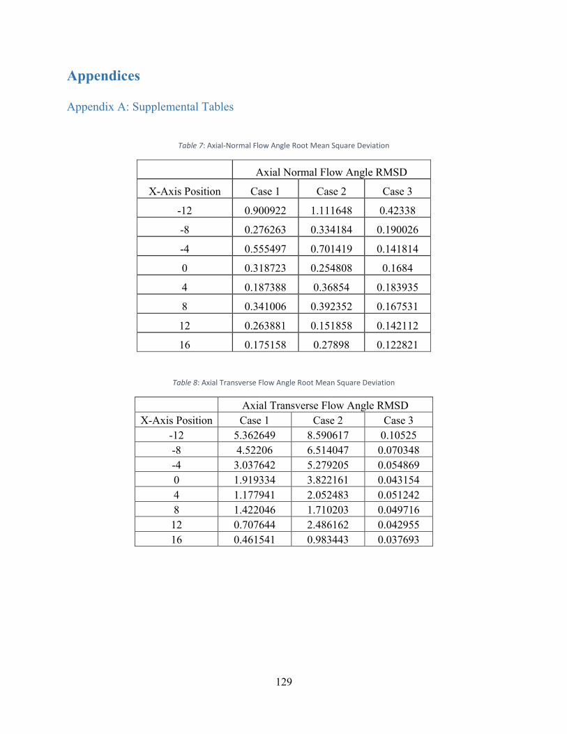
129
Appendices
Appendix A: Supplemental Tables
Table 7: Axial-Normal Flow Angle Root Mean Square Deviation
Axial Normal Flow Angle RMSD
X-Axis Position Case 1 Case 2 Case 3
-12 0.900922 1.111648 0.42338
-8 0.276263 0.334184 0.190026
-4 0.555497 0.701419 0.141814
0 0.318723 0.254808 0.1684
4 0.187388 0.36854 0.183935
8 0.341006 0.392352 0.167531
12 0.263881 0.151858 0.142112
16 0.175158 0.27898 0.122821
Table 8: Axial Transverse Flow Angle Root Mean Square Deviation
Axial Transverse Flow Angle RMSD
X-Axis Position Case 1 Case 2 Case 3
-12 5.362649 8.590617 0.10525
-8 4.52206 6.514047 0.070348
-4 3.037642 5.279205 0.054869
0 1.919334 3.822161 0.043154
4 1.177941 2.052483 0.051242
8 1.422046 1.710203 0.049716
12 0.707644 2.486162 0.042955
16 0.461541 0.983443 0.037693

130
Table 9: Stagnation Pressure Root Mean Square Deviation
Stag. P. Root Mean Square Deviation
X-Axis Position Case 1 Case 2 Case 3
-12 2.887433 2.791571 2.863307
-8 2.903745 2.845384 2.875512
-4 2.902201 2.8484 2.875999
0 2.891378 2.853025 2.863993
4 2.869229 2.853263 2.844766
8 2.8399 2.832913 2.819503
12 2.811158 2.830706 2.793984
16 2.773068 2.815657 2.762598
Table 10: Static Pressure Root Mean Square Deviation
Static Pressure RMSD
X-Axis Position Case 1 Case 2 Case 3
-12 0.016114 0.008042 0.037258
-8 0.012264 0.015858 0.024156
-4 0.008053 0.004822 0.007302
0 0.01537 0.003136 0.00108
4 0.011972 0.017963 0.001378
8 0.003431 0.005132 0.000477
12 0.007471 0.004868 0.000247
16 0.003648 0.007277 0.000271
Table 11: Entropy Root Mean Square Deviation
Entropy RMSD
X-Axis Position Case 1 Case 2 Case 3
-12 0.655825 0.727628 0.664299
-8 0.595287 0.67597 0.59747
-4 0.544203 0.620947 0.543706
0 0.506982 0.575383 0.500239
4 0.470033 0.550519 0.463676
8 0.435393 0.509955 0.430794
12 0.409724 0.4878 0.399633
16 0.379957 0.463285 0.369389

131
Table 12: Mach Number Root Mean Square Deviation
Mach Number RMSD
X-Axis Position Case 1 Case 2 Case 3
0 0.110982 0.102051 0.109352
4 0.119677 0.109368 0.115624
8 0.121677 0.108444 0.120701
12 0.122063 0.108777 0.12344
16 0.123035 0.107861 0.128647
Table 13: Stagnation Pressure Mass Weighted Average
Stag. P Mass Weighted Average
X-Axis Position Case 1 Case 2 Case 3
-12 3.791693 3.860969 3.797928
-8 3.687354 3.778725 3.693332
-4 3.589863 3.700373 3.595072
0 3.49884 3.625948 3.503020
4 3.412698 3.556225 3.416837
8 3.332055 3.48756 3.335741
12 3.255913 3.423362 3.258935
16 3.183297 3.361255 3.186079
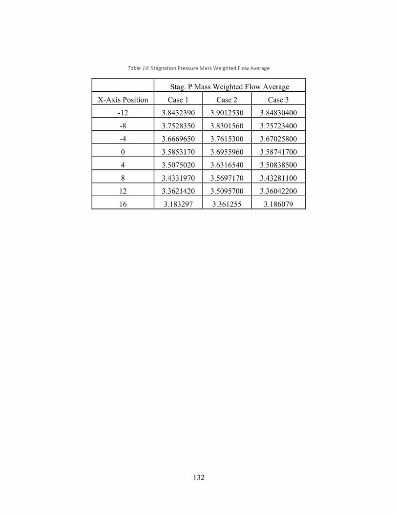
132
Table 14: Stagnation Pressure Mass Weighted Flow Average
Stag. P Mass Weighted Flow Average
X-Axis Position Case 1 Case 2 Case 3
-12 3.8432390 3.9012530 3.84830400
-8 3.7528350 3.8301560 3.75723400
-4 3.6669650 3.7615300 3.67025800
0 3.5853170 3.6955960 3.58741700
4 3.5075020 3.6316540 3.50838500
8 3.4331970 3.5697170 3.43281100
12 3.3621420 3.5095700 3.36042200
16 3.183297 3.361255 3.186079
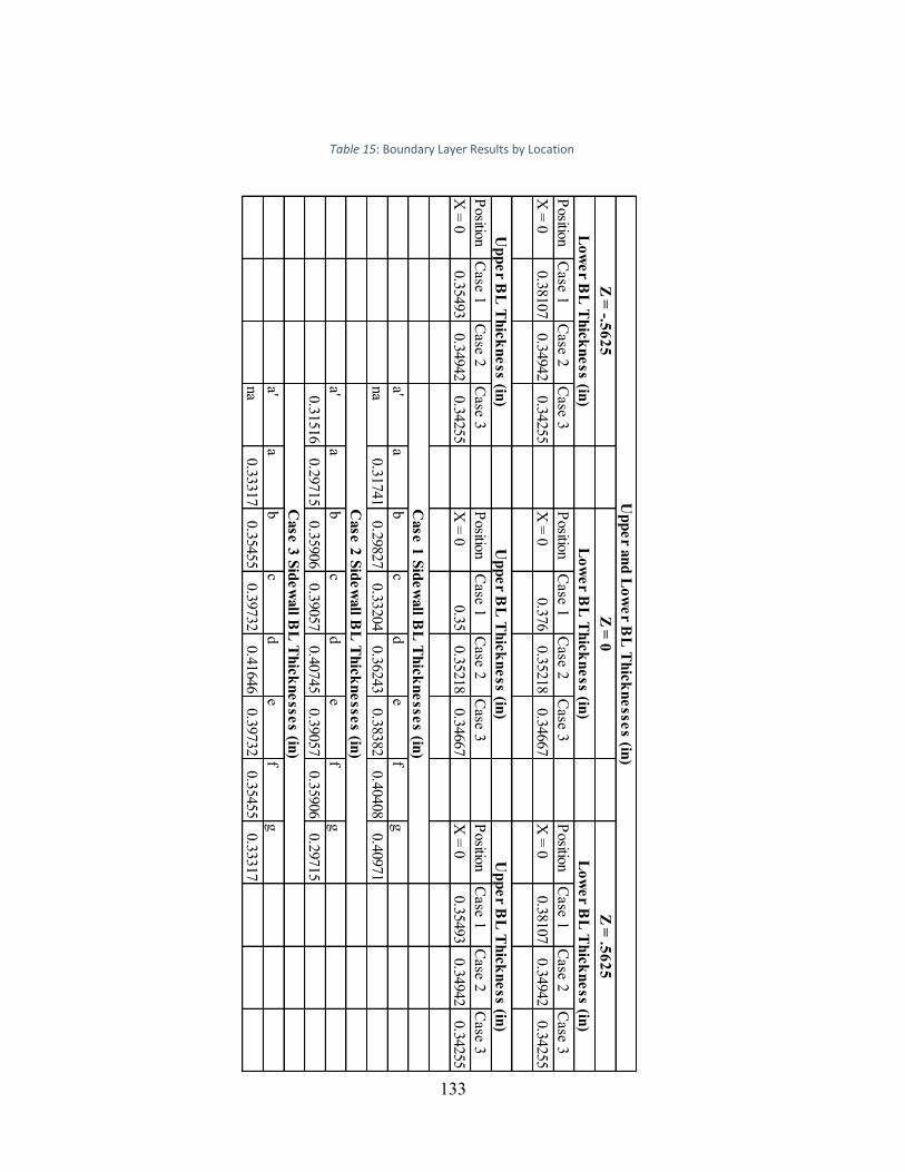
133
Positio
nC
ase
1C
ase
2C
ase
3P
ositio
nC
ase
1C
ase
2C
ase
3P
ositio
nC
ase
1C
ase
2C
ase
3
X =
00.3
8107
0.3
4942
0.3
4255
X =
00.3
76
0.3
5218
0.3
4667
X =
00.3
8107
0.3
4942
0.3
4255
Positio
nC
ase
1C
ase
2C
ase
3P
ositio
nC
ase
1C
ase
2C
ase
3P
ositio
nC
ase
1C
ase
2C
ase
3
X =
00.3
5493
0.3
4942
0.3
4255
X =
00.3
50.3
5218
0.3
4667
X =
00.3
5493
0.3
4942
0.3
4255
a'
ab
cd
ef
g
na
0.3
1741
0.2
9827
0.3
3204
0.3
6243
0.3
8382
0.4
0408
0.4
0971
a'
ab
cd
ef
g
0.3
1516
0.2
9715
0.3
5906
0.3
9057
0.4
0745
0.3
9057
0.3
5906
0.2
9715
a'
ab
cd
ef
g
na
0.3
3317
0.3
5455
0.3
9732
0.4
1646
0.3
9732
0.3
5455
0.3
3317
Case
1 S
ide
wall B
L T
hic
kn
esse
s (in
)
Case
2 S
ide
wall B
L T
hic
kn
esse
s (in
)
Case
3 S
ide
wall B
L T
hic
kn
esse
s (in
)
Up
pe
r BL
Th
ick
ne
ss (in
)U
pp
er B
L T
hic
kn
ess (in
)U
pp
er B
L T
hic
kn
ess (in
)
Z =
-.56
25
Z =
0Z
= .5
62
5
Lo
we
r BL
Th
ick
ne
ss (in
)L
ow
er B
L T
hic
kn
ess (in
)L
ow
er B
L T
hic
kn
ess (in
)
Up
pe
r an
d L
ow
er B
L T
hic
kn
esse
s (in
)
Table 15: Boundary Layer Results by Location

134
Table 16: Lower Wall Displacement Thickness at Z = 0 (inches)
Displacement Thickness (inches)
X-Axis Position Case 1 Case 2 Case 3
-12 0.039893 0.01233 0.038797
-8 0.041677 0.051758 0.050818
-4 0.05954 0.062336 0.062373
0 0.078718 0.067074 0.073509
4 0.085471 0.082852 0.083787
8 0.106098 0.085171 0.093689
12 0.117961 0.103097 0.103678
16 0.132217 0.112022 0.113562

135
Table 17: Blockage Data
Case 1
X Position
Blockage Area
(in2)
Blockage (% of
Tot. Area)
Unblocked area
(in2)
0 0.271344 4.38536 5.916156
4 0.295283 4.772246 5.892217
8 0.375214 6.064062 5.812286
12 0.476133 7.695076 5.711367
16 0.577334 9.330648 5.610166
Case 2
X Position
Blockage Area
(in2)
Blockage (% of
Tot. Area)
Unblocked area
(in2)
0 0.247374 1.998982 12.127626
4 0.264074 2.133934 12.110926
8 0.371878 3.005074 12.003122
12 0.44652 3.608244 11.92848
16 0.557449 4.50464 11.817551
Case 3
X Position
Blockage Area
(in2)
Blockage (% of
Tot. Area)
Unblocked area
(in2)
0 0.252213 4.076168 5.935287
4 0.287067 4.639469 5.900433
8 0.328441 5.30814 5.859059
12 0.385949 6.237552 5.801551
16 0.418157 6.758092 5.769343

136
Table 18: Axial Vorticity Root Mean Square Deviation
Vorticity RMSD
X-Axis Position Case 1 Case 2 Case 3
-12 5.146476 6.321854 2.055214
-8 1.186841 1.351967 0.663554
-4 2.6888 3.410832 0.517772
0 1.62301 1.142083 0.761998
4 0.653439 1.504917 0.867181
8 1.538156 1.893258 0.758335
12 1.244036 0.533156 0.611309
16 0.748491 1.143036 0.508192

137
Appendix B: Supplemental Figures
a) Case 1 b) Case 2
c) Case 3
Figure 55: V and W Velocity Vectors at x = 4

138
a) Case 1 b) Case 2
c) Case 3 Figure 56: V and W Velocity Vectors at x = 8