a novel screening method using score test for … · introduction methods results...

Introduction Methods Results Conclusions References

A Novel Screening Method Using Score Test for EfficientCovariate Selection in Population Pharmacokinetic Analysis

Yixuan Zou1, Chee M. Ng1

1College of Pharmacy, University of Kentucky, Lexington, KY

May 30, 2018


Outline

1 Introduction

2 Methods

3 Results

4 Conclusions


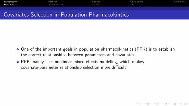
Covariates Selection in Population Pharmacokintics

One of the important goals in population pharmacokinetics (PPK) is to establishthe correct relationships between parameters and covariatesPPK mainly uses nonlinear mixed effects modeling, which makescovariate-parameter relationship selection more difficult


Score Test Introduction

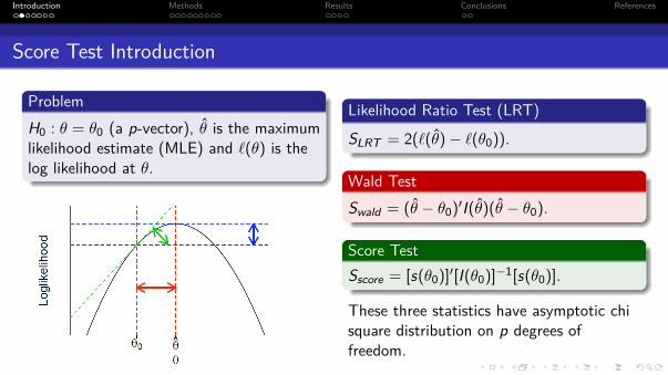
ProblemH0 : θ = θ0 (a p-vector), θ is the maximumlikelihood estimate (MLE) and `(θ) is thelog likelihood at θ.

Likelihood Ratio Test (LRT)

SLRT = 2(`(θ)− `(θ0)).

Wald TestSwald = (θ − θ0)′I(θ)(θ − θ0).

Score TestSscore = [s(θ0)]′[I(θ0)]−1[s(θ0)].

These three statistics have asymptotic chisquare distribution on p degrees offreedom.


Covariates Selection Method: LRT-based Stepwise Covariate Modeling(SCM)1

SCM: forward selection is followed with backward elimination based on LRTPros: It is still among the most popular methods to do covariate selection in PPKdue to good interoperability and relative economic computationCons: The model runs in NONMEM could be prohibitively large with large numberof covariates to be tested. The selection bias and inflated P-value are also issues

1Jonsson and Karlsson 1998.


Covariates Selection Methods: Wald Approximation Method (WAM)2

WAM: full covariate model fit to calculate the approximate LRT statistic for allpossible restricted models using Wald’s approximation. Final model is selected basedon the maximum (actual) Bayesian information criterion (BIC) derived fromNONMEM model fits for the 10–15 most probable models. It screens all possiblesubmodels only by fitting the full model with all covariates.

Pros: Fewer NONMEM runs (10-15) compared to SCMCons: A full covariate model with a covariance matrix is required, which is hard toobtain and MLE could be easily trapped into local minimum, so covariance matrixmay not be reliable even if it can be obtained

2Kowalski and Hutmacher 2001.


Other Covariates Selection Methods

There are other covariate selection methods, such as genetic algorithem (GA)3,LASSO4 etc. These methods are beyond the scope of this presentation. For a fulldicussion about the pros and cons of different methods, please refer to the referencedreview paper5

3Bies et al. 2006.4Ribbing et al. 2007.5Hutmacher and Kowalski 2015.


Covariates Selection Methods: Score Test-Based Covariate Method

Score test-based covariate method has never been used in PPK with nonlinearmixed effect modelingNo model fit is needed for score test after the base model has been successfullyidentified. It is potentially very useful to efficiently screen the potentialcovariate-parameter relationships in the presence of long model run due tocomplex population structural model and/or large number of tested covariates


Objective

The objectives wereTo conduct the type I error analysis and power analysis of score test in nonlinearmixed effect modelingTo develop the first score test-based covariate selection method in the PPK usingnonlinear mixed effects modeling approach


Score Test in Nonlinear Mixed Effects Model

NotationsAssume `(γ,θc) is the log likelihood function for a certain PPK covariate model,where γ = (θ,Ω,Σ), θ denotes fixed effects parameters for the base model, Ωdenotes the covariance matrix of inter-individual random effects, Σ denotes thecovariance matrix of intra-individual random effects, and θc denotes covariateparametersγ0 is the MLE of the model when θc = 0Score function is defined as S(γ,θc) = ( ∂`∂γ ,

∂`∂θc

)The observed fisher information matrix (negative hessian matrix) is

Iobs = −[

∂2`∂2γ

∂2`∂γ∂θc

∂2`∂γ∂θc

∂2`∂2θ

]


Score Test in Nonlinear Mixed Effects Model

Hypothesis TestingTo test H0 : θc = 0, the score statistic is

Sscore = S(γ,θc)′Iobs(γ,θc)−1S(γ,θc)|γ=γ0,θc =0,

since γ0 is the MLE under the H0, thus

Sscore = (0, ∂`∂θc|θc =0)′Iobs(γ0, 0)−1(0, ∂`∂θc

|θc =0),

Under H0 hypothesis and some regularity conditions, Sscore and LRT statistic have thesame asymptotic chi-square distribution.


Model Selection Criterion

Similar to BIC is penalized score chi square (ScoreP) used in the model selectionprocess.

Connection between BIC and ScorePBy omitting the constant term for each model,

BIC = −SLRT + klog(n) and ScoreP = −Sscore + klog(n),

where SLRT = −2(LLb − LLc), Sscore is the score statistic, LLb is the log likelihood forthe base model and LLc is the log likelihood for the covariate model, k is the numbercovariate parameters added in the model and n is the number of observations in thedataset.

↑ BIC and ScoreP → Model Performance ↓. We are going to use ScoreP to identifythe non-informative covariates.


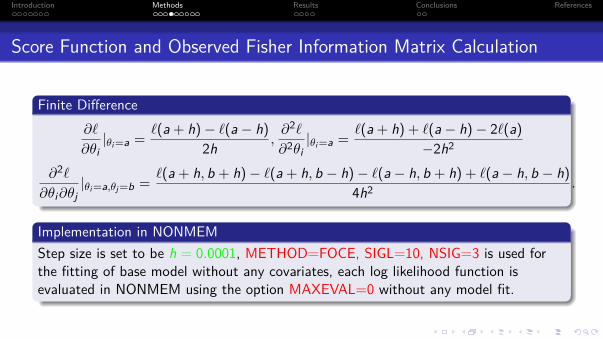
Score Function and Observed Fisher Information Matrix Calculation

Finite Difference∂`

∂θi|θi =a = `(a + h)− `(a − h)

2h ,∂2`

∂2θi|θi =a = `(a + h) + `(a − h)− 2`(a)

−2h2

∂2`

∂θi∂θj|θi =a,θj =b = `(a + h, b + h)− `(a + h, b − h)− `(a − h, b + h) + `(a − h, b − h)

4h2 .

Implementation in NONMEMStep size is set to be h = 0.0001, METHOD=FOCE, SIGL=10, NSIG=3 is used forthe fitting of base model without any covariates, each log likelihood function isevaluated in NONMEM using the option MAXEVAL=0 without any model fit.


Type I Error and Power Analysis of Score Test

One compartment PK model with IV bolusTypical values TVCL = 0.1L/h,TVV = 1.0LInter-individual variability ω2

CL = ω2V = 0.1

Intra-individual variability only has the proportional error σ2 = 0.1Sample size 50 and 200 with intensive sampling design (six sampling points persubject)Two types of analysis

Type I Error: The dataset was simulated without any covariates. The actualsignificance level6 for score test and LRT was compared using nominal significancelevels 0.1, 0.05 and 0.01Power Analysis: The dataset was simulated with covariate weight on clearance, thecovariate parameter is CLWT = 0.25, 0.75 respectively, the power of score test andLRT was compared using significance levels 0.1, 0.05 and 0.01

6Wahlby, Jonsson, and Karlsson 2001.


Type I Error and Power Analysis of Score Test

The actual significance level is calculated using the estimated upper tailprobabilities of the statistic S under null hypothesis H0 : θ = 0

Σ500i=1I[S > χ2

1(1− α)|H0]/500

The empirical power is calculated using the estimated upper tail probabilities ofthe statistic S under alternative hypothesis H1 : θ = θ0

Σ500i=1I[S > χ2

1(1− α)|H1]/500


All Possible Subset Screening Method Based on Score Test

Algorithm1 Identify the best base model without any covariates and fit the model in

NONMEM to get the MLE γ0

2 Add all the pre-specified covariate parameters into the base model and use finitedifference method to get the score function and observed Fisher informationmatrix for each parameter

3 Calculate the score statistic for each combination of covariates and thecorresponding ScoreP

4 Selection and elimination of the non-informative covariate models: Select themodel with the biggest ScoreP, which has the least information, the covariateswhich are not identified in the model are kept


All Possible Subset Screening Method Based on Score Test

Algorithm1 Identify the best base model without any covariates and fit the model in

NONMEM to get the MLE γ02 Add all the pre-specified covariate parameters into the base model and use finite

difference method to get the score function and observed Fisher informationmatrix for each parameter

3 Calculate the score statistic for each combination of covariates and thecorresponding ScoreP

4 Selection and elimination of the non-informative covariate models: Select themodel with the biggest ScoreP, which has the least information, the covariateswhich are not identified in the model are kept


Case Study Dataset Summary

Rituximab dataset was simulated with the original PK sampling design using themodel7:

N = 107 with IV rituximab 1000 mg on days 1 and 15On day 1, rituximab was given IV over about 255 minutes, and PK samples werecollected at predose, 3 hours, the end of infusion, and 6 and 48 hours after the startof the infusionOn day 15, the second dose was given IV over about 195 minutes, and PK sampleswere collected at predose, 3 hours, the end of infusion, and 6, 48, 336, 1088, 2352,and 3696 hours after the start of the infusion

7Ng et al. 2005.


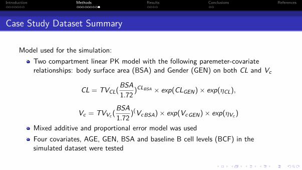
Case Study Dataset Summary

Model used for the simulation:Two compartment linear PK model with the following paremeter-covariaterelationships: body surface area (BSA) and Gender (GEN) on both CL and Vc

CL = TVCL(BSA1.72 )CLBSA × exp(CLGEN)× exp(ηCL),

Vc = TVVc (BSA1.72 )(Vc BSA)× exp(Vc GEN)× exp(ηVc )

Mixed additive and proportional error model was usedFour covariates, AGE, GEN, BSA and baseline B cell levels (BCF) in thesimulated dataset were tested


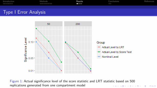
Type I Error Analysis

Figure 1: Actual significance level of the score statistic and LRT statistic based on 500replications generated from one compartment model


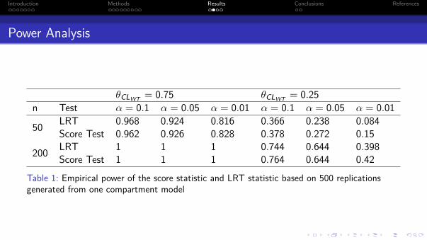
Power Analysis

θCLWT = 0.75 θCLWT = 0.25n Test α = 0.1 α = 0.05 α = 0.01 α = 0.1 α = 0.05 α = 0.01

50 LRT 0.968 0.924 0.816 0.366 0.238 0.084Score Test 0.962 0.926 0.828 0.378 0.272 0.15

200 LRT 1 1 1 0.744 0.644 0.398Score Test 1 1 1 0.764 0.644 0.42

Table 1: Empirical power of the score statistic and LRT statistic based on 500 replicationsgenerated from one compartment model


Model Screening Based on ScoreP

Rank by ScoreP Theta Selected ScoreP Score Chi Square BIC LRT Chi Sqaure Rank by BIC1 [CLAGE ,ClBCF ,Vc AGE ,Vc BCF ] 25.55 2.35 25.32 2.58 12 [CLAGE ,Vc AGE ,Vc BCF ] 20.63 0.30 20.56 0.37 23 [ClBCF ,Vc AGE ,Vc BCF ] 18.91 2.01 18.89 2.03 34 [CLAGE ,ClBCF ,Vc AGE ] 18.72 2.20 18.51 2.41 45 [CLAGE ,ClBCF ,Vc BCF ] 18.62 2.31 18.39 2.53 56 [Vc AGE ,Vc BCF ] 13.81 0.14 13.80 0.15 67 [CLAGE ,Vc AGE ] 13.78 0.18 13.71 0.24 78 [CLAGE ,Vc BCF ] 13.69 0.26 13.62 0.33 89 [CLAGE ,ClBCF ,Vc AGE ,Vc BCF ,Vc BSA] 12.71 22.17 4.75 30.13 1010 [ClBCF ,Vc AGE ] 12.10 1.85 12.08 1.87 9

Table 2: Ten worst models selected by ScoreP

The remaining covariate parameters, i.e. those that are not selected by this processCLBSA,ClGEN ,Vc BSA,Vc GEN are exactly the true covariates in the original model usedfor simulation; SCM approach with forward inclusion (p=0.05) and backwardelimination (p=0.01) also found the true covariates, but it took 38 NONMEM runs


Relationship between Score Chi Square and LRT Chi Square

Figure 2: LRT chi square and score chi square for the best 10 models and the worse 10 models


Discussion and Conclusions

Preliminary type I error and power analyses were conducted for score test underthe nonlinear mixed effects setting

Score test had comparable performance with LRT in power analysis, but had inflatedtype I error when sample size was smallRegarding to score test’s superior computational efficiency (no model fit is required),it may serve as a good screening tool in the forward selection step for SCM whendifferent forms of covariate parameters and large number of covariates need to betested instead of using LRT

A fast covariate screening method was proposed based on score test. It couldidentify those uninformative covariates all at once after base model was obtainedwithout any further NONMEM runsFurther study is ongoing on the validation process and the performance of thismethod in different scenarios with real clinical datasets


Thank You!


Bies, Robert R et al. (2006). “A genetic algorithm-based, hybrid machine learningapproach to model selection”. In: Journal of Pharmacokinetics andPharmacodynamics 33.2, pp. 195–221.

Hutmacher, Matthew M and Kenneth G Kowalski (2015). “Covariate selection inpharmacometric analyses: a review of methods”. In: British journal of clinicalpharmacology 79.1, pp. 132–147.

Jonsson, E Niclas and Mats O Karlsson (1998). “Automated covariate model buildingwithin NONMEM”. In: Pharmaceutical research 15.9, pp. 1463–1468.

Kowalski, Kenneth G and Matthew M Hutmacher (2001). “Efficient screening ofcovariates in population models using Wald’s approximation to the likelihood ratiotest”. In: Journal of pharmacokinetics and pharmacodynamics 28.3, pp. 253–275.

Ng, Chee M et al. (2005). “Population pharmacokinetics of rituximab (anti-CD20monoclonal antibody) in rheumatoid arthritis patients during a phase II clinicaltrial”. In: The Journal of Clinical Pharmacology 45.7, pp. 792–801.


Ribbing, Jakob et al. (2007). “The lasso—a novel method for predictive covariatemodel building in nonlinear mixed effects models”. In: Journal of pharmacokineticsand pharmacodynamics 34.4, pp. 485–517.

Wahlby, Ulrika, E Niclas Jonsson, and Mats O Karlsson (2001). “Assessment of actualsignificance levels for covariate effects in NONMEM”. In: Journal ofpharmacokinetics and pharmacodynamics 28.3, pp. 231–252.

a novel screening method using score test for … · introduction methods results...

Documents