1

A Novel Many-objective Evolutionary Algorithm Based on Transfer Matrix with Kriging model

Lianbo Ma a, Rui Wang a, Shengminjie Chenb, Xingwei Wang a, Chi Chengc, Zhiwei Lind,

Yuhui Shie

a College of Software, Northeastern University, Shenyang, China

bFaculty of Science, Kunming University of Science and Technology, Kunming, China

c School of Computer Science, Shaanxi Normal University, Xi’an, China d School of Computing, Ulster University, United Kingdom

e Southern University of Science and Technology, Shenzhen, China

Abstract: Due to the curse of dimensionality caused by the increasing number of objectives, it is very

challenging to tackle many-objective optimization problems (MaOPs). Aiming to alleviate the loss of selection

pressure in the fitness evaluation for MaOPs, this paper proposes a novel evolutionary optimization framework,

called Tk-MaOEA, based on transfer learning assisted by Kriging model. In this approach, in order to achieve

global space optimization, transfer learning is used as a map tool to reduce the objective space, i.e., devising

transfer matrix to simplify the optimization process. For the objective optimization, the Kriging model is

appropriately incorporated in order to further reduce computation cost. Accordingly, any EA-based paradigm or

search strategy can be integrated into this framework. Fast non-dominated sorting and farthest-candidate

selection (FCS) methods are used to guarantee the diversity of non-dominated solutions. Comprehensive

evaluations on a set of benchmark functions have been conducted to show that the proposed Tk-MaOEA is

efficietive for solving complex MaOPs.

Key Words: Evolutionary algorithm, Many-objective optimization, Transfer matrix, Kring model.

1. Introduction

Multi-objective optimization problems (MOPs) occur in many real-world applications, in which multiple

conflicting objectives need to be solved in order to find a set of optimal [1, 2]. Accordingly, the solutions to these

MOPs, referred as Pareto-optimal solutions (PS), denote a possible reasonable trade-off between all involved

objectives. And the image of PS in the objective space is known as Pareto front (PF) [3, 4]. When MOPs have

more than three objectives, they are called as many-objective optimization problems (MaOPs) [5-7]. As an

effective optimization paradigm for MOPs, the multi-objective evolutionary algorithms (MOEAs) have been

widely developed, being endowed with a powerful search ability to approximate the PF. However, most MOEAs,

2

especially inevitably suffer from severe degradation in performance on MaOPs [5-9]. This is caused by the

called curse of dimensionality w.r.t the difficulty of optimizing large number of objectives.

Experimental results [8, 9] have shown that traditional Pareto-dominance-based approaches, e.g., NSGA-II

[10] and SPEA2 [11], encounter several serious difficulties when dealing with MaOPs as following.

First, compared with 2- or 3-objective MOPs, the high-dimensional MaOPs would render the Pareto

optimality, which is unable to provide enough selection pressure to evolve the solutions towards the true PF. As

the number of objectives increases, most of the obtained solutions become non-dominated to each other very

quickly, resulting in the loss of selection pressure to drive the solutions to approximate the PF, which have been

reported well in the literatures [12,13]. When the number of objectives rises over five, the proportion of

non-dominated solutions in the population will reach more than 90% [14]. Thus, it is difficult to differentiate

preferred solutions from innumerable non-dominated solutions obtained during the search process. Moreover, the

many-objective optimization inevitably encounters the inability of exploring both convergence and diversity for

the approximation of the true PF.

Second, the extensive search in a high-dimensional space would seriously undermine the efficiency of

algorithmic operators, such as mating selection and variation [15]. As confirmed in [16, 17], in a variation

process, the new offspring produced by two nearly converged solutions, which are required to approach along its

original direction, would contrarily move far away the true PF. This causes the failure of the final population to

converge to the PF, despite spreading all over the objective space. As a result, the EAs for MaOPs (also called

MaOEAs) can only explore a limited region in a large search space, whereas being trapped in local segments of

the PF due to the invalid evolutionary operators.

In addition, due to the large search space, the diversity based selection criterion would be harmful to

facilitate the convergence of the obtained solutions, when it is activated in the selection process of

non-dominated solutions. For example, experimental results in [13] show that the diversity maintenance

mechanism in NSGA-II plays a negative role in the convergence performance on the 5-, and 10-objective

DTLZ2 instances.

There are also some other problems, such as visualization of multi-dimensional objectives, high computation

expense, and determination of an appropriate population size. Even if the PF is attainable, there are no effective

methods to visualize the front. A large number of solutions in the high-dimensional objective space need to be

selected and measured as the representations of PF, which is of computation cost.

In order to overcome the above difficulties, the dimensionality reduction scheme is naturally considered, to

reduce the number of objectives while trying to maintain the information of the objectives as much as possible.

3

For example, an effective approach, which uses the principle component analysis approach, has been proposed to

determine the correlation between lower dimensions of each objective [18]. This approach relies on iterative

progresses from the interior of the objective space towards the PF. A preset approximated front of

non-dominated solutions is used to determine the redundant objectives [19]. However, in many real-world

conditions, the problem's objectives sometimes cannot be reduced only according to the order of importance.

This causes the ineffectiveness of above methods. Furthermore, even if a relatively small number of objectives

can be reduced, it is not helpful to tackle the problem effectively in some specific cases.

This paper presents a new transfer learning method with Kriging model based MaOEA (Tk-MaOEA) without

any reference vectors or points in advance, in order to alleviate effect of the curse of dimensionality in MaOPs.

One of our main ideas is to reduce the complexity of large search space by using multi-dimensional compression

based on transfer learning. At the global space optimization level, a new transfer learning approach is proposed

to reduce the number of objectives, while the property of the objectives in the high-dimensional search space is

still kept during the transferring process. In the proposed approach, the redundant dimensions are compressed

using a transfer matrix with Gram-Schmidt orthogonalization. At the objective optimization level, Kriging

models are utilized to reduce the number of expensive evaluations by approximating each objective value. By

using these mechanisms, we can follow the idea of improving the effectiveness of Pareto optimality and

overcoming the difficulty of the extremely large search space.

In Tk-MaOEA, the primary principle is to use transfer matrix for dimensionality reduction to enforce the

population evolution to be limited in a low-dimensional search space. As a result, the simplified optimization in

the small objective space not only guarantees the effectiveness of conventional evolutionary operators, but also

facilitates improving the performance of Pareto optimality. Afterward, when optimizing the simplified

low-dimensional MaOP, the Kriging model is constructed for each objective to enhance the objective

optimization, by using the Latin hypercube sampling (LHS) method. In this proposed design, the transfer

learning and Kriging model with FCS strategy perform distinctly, yet complementarily. Transfer learning offers

the convergence power, while the FCS assisted by Kriging model enhances the primary diversity power.

Generally, the conventional work only focuses on the monotonous combination of surrogate models into

conventional EA algorithms. In contrary, our design focuses the importance of the combinational contribution of

the Kriging and transfer learning to the optimization goal. Tk-MaOEA utilizes and maximizes the benefits of

Kriging model to assist the dimensionality reduction scheme for complex many-objective optimization. Our

contributions mainly include:

1) At the global space optimization level, a new transfer learning approach is developed to reduce a large

4

number of objectives while the original property of the problem is kept well. The proposed approach uses a

specific transfer matrix to compress the search space, which is simple yet effective to handle with the curse of

dimensionality in MaOPs.

2) At the objective optimization level, the Kriging model is devised for each objective to further reduce

computational cost. This Bayesian based surrogate model is to measure not only the objective value itself but

also stochastic error of the approximation, which is essentially conductive to improve the accuracy of the

optimization.

3) The multi-scale normalization approach is employed so as to avoid the distortion caused by conventional

normalization in the high-dimensional objective space. This is a significant operation for the MaOEA to keep

unchanged spatial distribution when the original population are normalized.

4) The FCS approach is incorporated instead of the traditional crowding distance method in the

environmental selection. This approach is more effective to select a set of representative non-dominated

solutions in a single run.

The remainder of this paper is organized as follows. Section 2 elucidates related works. In Section 3 the

proposed algorithm is given in detail. In Section 4, the experiment is conducted on a serial of well-defined test

functions. Finally, Section 5 outlines the conclusions.

2. Related works

2.1 Many-objective optimization

An MOP with only box constraints is defined as follows:

(1)

where x=(x1,…,xn) is n-dimensional decision vector from the decision space Rn; F: Rn→Rm is a mapping function

from Rn to an objective space Rm, involving m objectives; k and q are the number of inequality and equality

constraints, respectively. If m >3, the problem is also referred as a MaOP.

1) Given two solutions X1, X2 Rn, X1 dominates X2, i.e., X1 X2, if i {1,2,...,m}, fi(X1) fi(X2) and

i {1,2,...,m}, fi(X1)<fi(X2).

2) Any solution x Rn can be referred as a Pareto-optimal solution or non-dominated solution if no other

feasible solutions dominate x in Rn.

3) The set of all Pareto-optimal solutions in the objective space is said to be the Pareto set (PS), and the plotted non-dominated solutions or PS is called the Pareto front (PF), i.e., .

To tackle these MaOPs, many MaOEAs have been developed deliberately, including the following classes.

1Minimize ( ) ( ( ), , ( ))( ) 0, 1,2, ,

s.t. ( ) 0, 1,2, ,

mx

i

j

F x f x f xg x i kh x j q

= …³ =ì

í = =î

!!

Î ! " Î £

$ Î

Î

1: {( ( ), , ( )) | }kPF f x f x x PS= … Î

5

First, decomposition-based algorithms divide a complex MaOP into a set of scalar sub-problems and solve

them in a cooperative manner. For example, MOEA/D [20] uses the weighted sum or Chebyshev method to

select individuals for next generation, while the neighborhood of subproblems are incorporated. Then, several

variants have been proposed [17, 21, 22]. Reference [17] develops a new double-level archive mechanism based

on the framework of MOEA/D to maintain both convergence and diversity of solutions, and reference [11]

proposes an improved MOEA/D variant called MOEA/D-EGO to reduce the computation cost.

The second approach is based on the idea of quality indicators. These indicators can be directly used as the

fitness assignment to guide the evolutionary process. IBEA [23] has exhibited a prominent ability of converging

to PF at a high pace. However, the diversity of population is not maintained appropriately [23]. Accordingly, a

novel indicator S is used to improve the convergence and diversity simultaneously [24]. Likewise, in [25] an

effective indicator R2 is proposed in MOMBI. Another interesting approach, the hypervolume (HV), can measure

both the convergence and diversity, but it consumes much computation cost [26].

The third one is the relaxed dominance based approach. Those algorithms strike to alleviate the inefficiency

of Pareto dominance via enhancing the selection pressure, such as Pareto ε-dominance [27], Pareto α-dominance

[28] and controlling Pareto dominance area [29]. It has been validated experimentally that these approaches are

more effective than traditional Pareto dominance. Furthermore, for the augment of selection pressure, several

new strategies are developed to make a solution be dominated by others more probably. The prominent examples

include fuzzy-Pareto dominance [30], L-optimality [31], and ranking method [32]. Among those, one excellent

approach GrEA [33] uses a grid-based measurement to differentiate and select the non-dominated solutions. In

[34], a new farthest-candidate approach is proposed to replace the crowding distance mechanism in NSGA-II,

and it is more effective to maintain the diversity of population.

There are also some other hybrid algorithms, such as NSGA-III [35] and the improved two-archive MaOEA

[36]. In NSGA-III, a number of well-distributed reference points are initialized to guide the population along

specific directions for maintaining good diversity [35]. The improved two-archive cooperation mechanism

proposed in [36] respectively assigns two different indicators to the two archives in order to handle with the

convergence and diversity separately. Other approaches based on reference vectors or preference information

have been proposed and developed well [37-40].

2.2 Dimensionality reduction

In many-objective optimization, the dimensionality reduction technique aims to identify the potentially least

amount of objectives to characterize the original optimization problem adequately [41-45]. Up to now, a variety

6

of valuable dimensionality reduction approaches have been developed.

The first one is based on the idea of dominance relation preservation. Reference [41] proposes an effective

objective reduction approach by preserving the dominance relations in the obtained PS. Specifically, given an

objective f F (i.e., the objective set), if the dominance relations between objectives keep constant when f is

deleted, then f is regarded to be non-conflicting with the other members in F. Furthermore, a novel greedy

algorithm is developed to resolve δ-MOSS and k-EMOSS problems [41]. In [42], the conflict and non-conflict

dominance relations between each pair of objectives are fist analyzed and then the non-conflicting ones are

identified and amalgamated into one objective.

The second class is unsupervised feature selection. In [43], the objective correlation is analyzed, and then

the objectives with more distance to each other are processed as the more conflicting ones. In this approach, the

objective set is grouped into a set of neighborhood subsets with the size q near each objective, and the

neighborhood with the most compact structure is selected preferentially, whose central node is acquired and the

corresponding neighbors are removed. Based on above paradigms, two algorithms have been developed to

tackleδ-MOSS and k-EMOSS problems [43].

The third one is the called Pareto corner search. Based on this principle, the algorithm in [44] explores only

the corner segmentation of the PF, instead of searching for the entire PF. In this approach, the obtained

non-dominated solutions are supposed to properly acquire the feature of the PF on each objective. Then the

dimensionality reduction is accomplished with the assumption that it is acceptable to eliminating a redundant

and an essential objective.

The forth type is machine learning based dimensionality reduction. The new approaches in [45,46] take

advantage of machine learning mechanism including principal component analysis (PCA) and maximum

variance unfolding (MVU) to determine the priority of the dependences in the non-dominated solutions.

Essentially, this scheme is based on the principle that high-dimensional solution structure can be well captured

via minimizing the effect of noise and dependencies.

Furthermore, several nonlinear dimensionality reduction approaches have been developed, such as kernel

PCA [47] and graph-based algorithm [48]. Reference [49] introduces a graph-based method into the MVU

mechanism, within which the low-dimensional representation is tackled by gradually unfolding the

high-dimensional information manifold. In this method, the unfolding is accomplished according to the

Euclidean distances between points while the distances, with the preservation of distances and angles between

adjacent points.

Î

7

2.3 Surrogate models

Recently many surrogate models have been employed to assist EAs as state-of-the-art search strategies

[50-54]. For example, reference [51] proposes a surrogate model-aware search mechanism for medium scale

computationally optimization problems, i.e., 20-50 decision variables, and a comparative study about

surrogate-assisted multi-objective EA framework is conducted in [53]. These surrogate-assisted algorithms are

able to effectively seek multiple optima and reduce the number of function evaluations by using information

provided by surrogate models, e.g., Kriging methods [55–58]. These surrogate models may need additional

computation costs and high usage of memory. It is stressed that these methods are increasingly useful as the

problem complexity increases, because the computational cost caused by Kriging models is much less than that

for function evaluations [59,60]. Hence, the surrogate models have significant potential to assist the

dimensionality reduction scheme for many-objective optimization.

Algorithm 1 Main Framework of Tk-MaOEA

Input: N (population size), Max_Gen ( the maximum number of generations), TN(after transfer objectives number )

Output: P (final population)

1: /* Initialization */

2: Randomly initialize a population P0 with N individuals

3: Trt = zeros(N, TN)

4: /* Main Loop */

5: While t ≤ Max_Gen do

6: P't = Mating Selection(P,B)

7: Qt = Variation(P't)

8: S = Pt � Qt

9: T=Transfer matrix(Pt, TN)

10: Trt = St * T

11: Multi-scale normalization(Trt)

12: Totalt=[Pt, Trt]

13: P = Environmental Selection (Totalt)

12: t + +

13: End While

3. Proposed algorithm

3.1 Basic idea

Our approach uses transfer matrix based space reduction to drive the population to move in a relatively low

8

dimensional search space, and then utilizes Kriging-assisted mechanism for each objective to enhance the

exploration ability, based on the Latin hypercube sampling (LHS) method. In order to retain fast convergence as

well as even distribution of the solutions, the farthest-candidate selection (FCS) is incorporated based on the fast

non-dominated sorting approach in the environmental selection. As shown in Algorithm 1, the main framework

of Tk-MaOEA is composed of the following components. First, in the initialization, N individuals are initialized

randomly to form a parent population (Lines 1-2 in Algorithm 1). Second, a binary tournament strategy is

adopted to select solutions from the parent population to generate an offspring population Q with N individuals

using a variation operation (Lines 6-8 in Algorithm 1). The variation operation employs conventional crossover

and mutation used in [10]. Then, the combined population is transformed via transfer matrix to low dimensional

objective space (Lines 9-12 in Algorithm1). Finally, N solutions are selected from the combined population in

the environmental selection procedure (Line 10 in Algorithm 1). In this procedure, the FCS method is employed

to select elite individuals to maintain diversity of solutions for the next generation. These procedures repeat until

a termination condition is me. The following subsections will show their details.

Algorithm 2. Transfer matrix

Input: P(population), TN(after transfer objectives number )

Output: transfer Matrix T

1: /*find the best individual */

2: p*={p|best(P)}, p P

3: p*=normalization(p*)

4: While i< TN do

5: /* find the linearly independent unit vectors et with p* */

6: p*= p* et

7: i++

8: End While

9: p*T =Gram-Schmidt Orthogonalization(p*T)

10: T=[p*T]

11: Return T.

3.2.Transfer Matrix

Algorithm 2 shows the main principle of transfer matrix. For each generation, the best Pbest is firstly selected

(Lines 1-3 in Algorithm2). Then, the TN-1 linearly independent unit vectors are determined according to the Pbest

(Lines 4--7 in Algorithm2). As a result, the transfer matrix is constructed to makes up with TN linearly

independent column vectors. Next, the Gram-Schmidt Orthogonalization method is adopted for the

Î

!

9

orthogonalization of each column vector in the matrix, as shown in Algorithm 3. Accordingly, the first column in

the transfer matrix is the best individual direction and other columns are the orthogonal direction with best

individual, and each column is an unit. Theoretically, this transfer matrix can guide the other members in the

population to learn from the best individual (refer to the proof of Theorem1 and Theorem 2 in Appendix).

That is, the map lengths in the best individual direction and in the vertical individual direction can be used in the

transfer learning. Therefore, a large number of objectives can be represented by a relatively small number of

objectives, in virtue of the map length in the best individual direction and the map length of the other vertical

individual direction.

In Euclidean space, it is desired that linearly independent vectors are transformed to orthogonal vectors. For

this purpose, the Gram-Schmidt Orthogonalization (GSO) operation is devised as shown in Algorithm 3. First,

each vector in the orthogonal vector group should be normalized (Lines 2 and 5 in Algorithm 3). Next, the GSO

operation is implemented by using a linear combination of the inner product (Line 4 in Algorithm 3). Finally, the

orthogonalized vector group is obtained, which will play a positive role on the algorithm.

Algorithm 3. Gram-Schmidt Orthogonalization

Input: X(matrix)

Output: Matrix X*

1: x1*=x1 /* X=[x1,x2,...,xTN] */

2: x1*=normalization(x1

*)

3: While i< TN do

4: x1*=xi -

5: xi*= normalization(xi

*)

6: i++

7: End While

8: X*=[x1*,x*

2,...,xTN*]

9: Return X*.

3.3 Multi-scale nomination

In the algorithm, it is desired to map them from a scaled objective space onto a normalized objective space.

Note that, in many MaOPs such as WFG problems [50] and scaled DTLZ problems [51], their objective values

are usually scaled disparately. In this case, the conventional normalization will generate a set of distorted

solutions, whose spatial distribution is not consistent with the original ones. Therefore, as suggested in [52],

1

1

,,

ii j

jj j j

x xx

x x

*-*

* *=å

10

instead of normalizing the objectives, we use the Schur product to translate fi*(x) to Fi(x) according to the

boundary range of the objective values, as

(2)

where fi'(x)=f(x)- zimin is the ith translated objective value, zimin and zimax are the ith ideal point and the ith nadir

point, respectively. The binary operator denotes the Schur product, which takes two matrices of the same

dimensions, and produces another matrix where each element is the product of elements of the original two

matrices.

Algorithm 4 Environmental selection

Input: P (combined population)

Output: P' (new population)

1: P =∅, i=1;

3: (F1,F2,...) = Non-dominated-sorting (P)

4: While |P|+|Fi|<N+1

5: P= P Fi and i=i+1

6: End While

7: The last front to be included Fl=Fi

8: If |P| = N

9: return P

10: Else

11: /* Apply FCS strategy */

12: Solutions to be selected from Fl: K=N-|P|

13: Choose K solutions one by one from Fl to form the final P'.

14: End If

15: Return P'

3.4 Environmental selection

Algorithm 4 illustrates the framework of environmental selection. Intuitively, this framework takes into

consideration both the convergence and diversity of solutions, which are obtained by the Kriging-assisted

mechanism and the FCS method, respectively. First, the traditional fast nondominated sorting is utilized to

divide current solutions into different layers, and then the last layer Fl is determined (lines 3–6 in Algorithm 4).

If the population size is equal to N, then return P. Otherwise, K (N −|P|) solutions from Fl are selected into P one

by one by using the called FCS approach (lines 11-13 in Algorithm 4), as presented as below in details.

3.4.1 The FCS approach

*

*

'( ) ( - )( )|| '( ) ( - ) ||

nadi

i nadi

f x z zF xf x z z

=!!

!

!

11

In Tk-MaOEA, instead of the traditional crowded distance method [10], an improved selection approach FCS,

is devised, as suggested in [64]. Its main procedures is shown in Algorithm 5. In principle, the unselected

individuals with farthest Euclidean distance from current selected solutions are selected preferentially as

candidates. Specifically, in order to select K elite individuals from the population, the boundary individuals with

the smallest and largest fitness values are selected into the group of selected individuals (Lines 1-4 in

Algorithm5). Then, the Euclidean distance between each solution and unselected ones are calculated and the

minimum values of Euclidean distance are memorized (Lines 5-7 in Algorithm5). Finally, the farthest solutions

are selected into Saccept (Lines 8-11 in Algorithm5).

Algorithm 5. The FCS method

1: Saccept = ;

2: D[xi]=0, i=1,2…, N;

3: For each objective function fj(x), j=1,2…,m

4: Saccept = Saccept (fj(x)) (fj(x));

5: Let Sm[x]=P-Saccept, for each individual x Sm,

6: D[xi] (dis(x,x’));

7: For i=1 to K-|Saccept|

8: x1= (D[x]);

9: For each x2 P-Saccept

10: D[x2] min(D[x2],dis(x,x’));

11: Saccept Saccept x1

12: End For

13: End For

Fig. 1. Reference point definition using a ideal point of solutions on the Kriging models

f

! argminx PÎ

! argmaxx PÎ

Î

'arg min

acceptx Sά

( )arg max

acceptx P SÎ -

Î

¬

¬ !

the initial individuals

Non-dominant front on the Kriging models

f1

f 2

12

Fig. 2. Illustration of solutions selection by FCS and CD

The aim of the FCS method is to solve difficulties encountered by the crowded distance (CD) mechanism in

particular situations where the solutions are not well-distributed. Take an example to illustrate, Fig. 2 shows 12

solutions to be proceeded by optimizers, and most of them are very close to each other whereas the others are not.

In this case, optimizers need to select 5 solutions from 12 solutions. These selection results obtained by FCS and

CD are identified by red and green, respectively. It is apparent that the spread of solutions obtained by FCS is

significantly better than that obtained by CD. This is because in the CD selection, the solution with a high

density has a low chance to be selected, which may damage the spread of selected solutions. Fortunately, the

FCS method can avoid this dilemma by using the principle of best-candidate sampling theory.

3.4.2 Enhanced objective optimization based on Kriging model

In Tk-MaOEA, the Kriging model is used for each objective function when the initial population is generated.

Especially, following the approach in [65], the Kriging model is constructed by interpolating a number of

uniformly-distributed individuals, initialized by Latin hypercube sampling (LHS) method [65]. Then, in the

environmental selection process, the preferred solutions are selected from the Kriging model according to the

estimated objective functions, as shown in Fig.1.

The ordinary Kriging model represents the unknown function f (x), which is formulated as

(3)

where x is an m-dimensional decision vector, a(x) is a global model, and b(x) is a Gaussian process with N(0, σ2),

which represents a local error with the global model. The correlation between b(xi) and b(xj) is strongly

correlated to the distance between xi and xj. Here, we use the Gaussian function with a weighted distance to

define the correlation as

(4)

where (0 ≤ < ∞) is the weight factor of the kth element of an m-dimensional weight vector . These

weights maintain the anisotropy of the Kriging model and improve its accuracy. The predictor and uncertainty of

1 23 45

1 23 4 5

FCS

CD

)()()( xbxaxf +=

))(exp())(),((1

2å=

--=m

k

kj

ki

kji xxxbxbCorr w

kw kw w

13

the Kriging are expressed as

(5)

(6)

where is the approximated value of b(x), R expresses the matrix whose (i, j) element is

Corr(b(xi),b(xj)), r(x) is an n-dimensional vector whose ith element is Corr(b(xi),b(xj)), and then f and are

formulized as follows when there are n solutions

(7)

(8)

and , and (approximated ) are the unknown parameters in the Kriging model. By maximizing

the likelihood function, the unknown parameters are obtained [65].

Based on the Kriging model, the EI value, which is the expected objective function improvement from the

current non-domination solution, is calculated according to the improvement value I(x), expressed as

(8)

(9)

where is the probability of f, whose density function is , fref is the reference value of f, i.e.,

minimum value of f(x). Accordingly, EI(x) can be treated as the approximated value of the objective function.

Finally, the Kriging model is easily incorporated and implemented on each objective function in Tk-MaOEA.

4. Experimental results

In this section, the experimental study is conducted to evaluate the performance of the proposed Tk-MaOEA.

Tk-MaOEA is benchmarked against a set of test functions including DTLZs [70] and WFGs[61], with several

popular MaOEAs, namely MOEA/D [20], NSGA-III [35], MOMBII [25] and VaEA [7]. These algorithms have

been verified to be effective on MaOPs, and they can be grouped into three classes: 1) the reference points or

weight vectors based algorithms (MOEA/D and NSGA-III), 2) indicator based algorithm (MOMBII) and 3)

Pareto dominance based algorithm (VaEA). The principal description of MOEA/D, NSGA-III, and VaEA can be

referred in Sections I or their original literature [8, 35, 7]. MOMBII, as a recently proposed indicator based

algorithm, takes a less-computation indicator called R2 as the selection criterion, which essentially weakens the

Pareto compatibility [66]. Detailed presentation can be referred in reference [66].

1( ) ( ) ( ) ( )Tf x b x r x R f b-= + -! ! !

1 22 2 1

1(1 1 ( ))( ) (1 ( ) ( ) )

1 1

TT

T

R r xv x r x R r xR

s-

--

-= - +!

( )xb! n n´

b!

1( (x )... (x ))n Tf f f=

1( )... ( ))( n Tx xb b b=! ! !

w ( )xb! 2s! 2s

(x) max( ,0)refI f f= -

(x) ( )reff

refEI f f (f)dfl-¥

= -ò

l ! 2( ), ( )( )x v xfN

14

4.1 Test Problems and Performance Measures

The first 4 instances (DTZL1 to DTLZ4) are taken from DTLZ [70]. where the number of decision variables is

set to n = M + r − 1, where M is the objective number, r = 5 for DTLZ1, and r = 10 for DTLZ2 to DTLZ4. The

other 9 test instances (WFG1 to WFG9) are taken from WFG [61], where the number of decision variables is set

to n = k+l−1. As recommended in [61], the distance-related parameter l is set ot10 and the position-related

parameter k is set to 4, 10, 7, and 9 for test instances with M = 3, 5, 8, 10, respectively. The attributes of involved

problems include separability or nonseparability, unimodality or multimodality, unbiased or biased parameters,

and convex or concave geometries. In order to quantitatively evaluate the performance of our proposed

algorithm, two performance metrics are adopted: 1) convergence metric-IGD metric [67]; 2) hypervolume

metric- Hv [57]. The further information about the two performance metrics can be referred in [67, 68]. Note that,

as stated in [67], the number of reference points for computing IGD should be large enough so as to cover the

complete PF as well as possible. Thus, the numbers of divisions for different numbers of objectives for DTLZs

and WFGs are respectively listed in Table 1 and Table 2, where the last column shows the number of reference

points for the problems. In addition, in order to indentify the significance of performance difference between

those results obtained by Tk-MaOEA and its counterparts, Wilcoxon’s rank sum test [69] is applied to obtained

results with a level of significance a=0.05.

Table 1 Number of reference points for DTLZs

M h1(P) h2 Number of reference points

3 25 - 351

5 13 - 2380

8 7 6 5148

10 6 5 7007

Table 2 Number of reference points for WFGs

M WFG1 WFG2 WFG3 WFG4-9

3 421 148 5000 351

5 2801 1601 17000 2380

8 5464 4690 15000 5148

10 20705 13634 26000 7007

4.2 Experimental Configuration

The recommended parameter values for the algorithms that have obtained the best performance are

configured as below.

15

1) Population size: for MOEA/D and NSGA-III, the population size is set empirically according to the

simplex-lattice design factor H together with the objective number M. For VaEA, as recommended in [7], its

population size keeps the same as that of NSGA-III. For the other two algorithms, Tk-MaOEA and MOMBII,

the population sizes are set to the same as that of NSGA-III and MOEA/D, with respect to different objective

numbers M.

2) Crossover and mutation: The SBX and polynomial mutation are used and the distribution indexes of

crossover and mutation are set to nc = 20 and nm = 20, respectively. The crossover probability pc = 1.0 and

mutation probability pm = 1/D, where D is the number of decision variables.

3) Number of runs and termination condition: Each algorithm is performed for 20 independent runs on

each test instance and the maximum function evaluations (MFEs) is set to 400000. For VaEA, the termination

condition can be determined by Gmax = MFE/N, where N is the population size.

4) Other parameters: For MOEA/D, the Tchebycheff approach is used with neighborhood range set to

N/10 where N is the population size. For MOMBII, involved parameters are set as =1e-3 andα = 0.5. For

Tk-MaOEA and VaEA, their parameters are set to the same as that of NSGA-III [10].

4.3 Results and Analysis

The experimental results of all algorithms over 3-, 5-, 8-, 10-objective test benchmarks are given in Table 3,

Table 4 and Table 5. In these tables, the mean and standard deviation (SD) values in terms of the HV and IGD

metrics obtained by the MaOEAs over 20 independent runs are reported. The significance of difference between

Tk-MaOEA and the compared algorithms is evaluated by Wilcoxon’s rank sum test.

4.3.1 Results in terms of HV metric

As shown in Table 3, Tk-MaOEA is the most effective performer, which achieves the first or second ranks on

most of DTLZ test instances. NSGA-III and VaEA also obtain satisfactory performance. Specifically, NSGA-III

obtains the first ranks on 8-, 10-objective DTLZ1, 5- and 8-objective DTLZ2, while VaEA is ranked the first on

5-objective DTLZ3 and 8-objective DTLZ4. MOMBII and MOEA/D obtain similar performance, doing well on

low-dimensional instances, such as 3-objective DTLZ1 and DTLZ4. In fact, the statistical results in terms of

IGD values for all the algorithms are close to each other.

As for the WFG instances, it can be observed from Table 4 that Tk-MaOEA performs very powerfully,

retaining the first or second ranks on most of test instances. As shown, both Tk-MaOEA and NSGA-III perform

powerfully, exhibiting an obvious superiority to other involved algorithms on the majority of the WFG test

instances. Specifically, Tk-MaOEA obtains the first and second ranks in terms of HV values on 17 and 6 out of

e

16

the 36 test instances, respectively. At the same time, NSGA-III obtains 10 first-rank results on all test instances

while MOMBII and VaEA also retains the fist ranks on 6 out of the 36 test instances. On 8-objective WFG3 and

8-objective WFG8, MOEA/D does very competently, ranked the first. For 5-objective WFG3, 3-objective

WFG7 and 8-objective WFG7, VaEA performs only slightly better than Tk-MaOEA.

For WFG1, NSGA-III performs the best, but just only a little better than Tk-MaOEA. In fact, the difference

between their mean results are very close. On WFG2, Tk-MaOEA does the best on 8- and 10-objective instances

while NSGA-III performs best on 5-objective instances. In fact, on 10-objecitve WFG2 instance, the

performance of Tk-MaOEA is significantly better than that of NSGA-III. It should be stressed that the

performance of Tk-MaOEA is not deteriorated when the number of objectives increases, unlike other algorithms.

MOMBII also achieves the best performance on 3-objective WFG2. On WFG3, all the involved algorithms

except NSGA-III obtain similar performance on 3- and 8-objective instances. Tk-MaOEA obtains the first rank

on the 10-objective instance, while MOEA/D also performs very powerfully on this instance. As the number of

objectives becomes large (i.e., M=8 and M=10), the performance of MOMBII seem somewhat worse than that of

NSGA-III and Tk-MaOEA .

For WFG4, whose PF has many local optima to be difficult to optimized. Tk-MaOEA obtains the first or

second results on 3 out of the 4 test instances, which are 8- and 10-objective, and MOMBII also finds the best

result on the 3-objective instance, but struggle on the higher-dimensional cases. For WFG5, Tk-MaOEA

performs most powerfully, ranked first on most of the test instances. For nonseparable WFG6, Tk-MaOEA

obtains a satisfactory performance, only worse than that of NSGA-III on 8-objective instance. Similar

observation are obtained on WFG7, which is the separable and unimodal problem, Tk-MaOEA does better or at

least comparably to VaEA, yet superior to other algorithms. On nonseparable WFG8, similar to the WFG6 case,

Tk-MaOEA is the best performer on most of test instances, and only slightly worse than NSGA-III on

3-objecitve instances. On WFG9, NSGA-III obtains satisfactory performance, only worse than Tk-MaOEA on

the 3- and 10-objective instances, while VaEA does best on 8-objective instance. These results show the

effectiveness of the proposed strategies in Tk-MaOEA

17

Table 3 Mean and standard deviation results of HV obtained by Tk-MaOEA, MOEA/D, MOMBII, VaEA and NSGA-III on DTLZs1-4 (The best items are in bold).

Problem M Tk-MaOEA MOEA/D MOMBII VaEA NSGA-III

DTLZ1

3 8.793e-01/4.175e-02 8.417e-01/8.374e-06+ 8.416e-01/3.096e-05+ 8.300e-01/4.906e-03+ 8.413e-01/2.375e-04+

5 8.793e-01/1.416e-01 9.704e-01/8.132e-05- 9.706e-01/1.117e-04- 8.833e-01/3.778e-02- 9.705e-01/4.808e-05-

8 9.752e-01/1.003e-02 9.753e-01/8.447e-04- 6.285e-01/2.276e-01+ 8.799e-01/2.585e-02+ 9.896e-01/7.156e-04-

10 9.194e-01/3.035e-02 9.951e-01/4.759e-04- 7.575e-01/2.841e-02+ 9.280e-01/5.252e-02- 9.983e-01/1.817e-02-

DTLZ2

3 5.233e-01/5.110e-02 5.596e-01/1.265e-06- 5.595e-01/5.118e-05- 5.558e-01/1.409e-03- 5.596e-01/2.708e-06-

5 7.075e-01/8.613e-02 7.743e-01/4.455e-04- 7.745e-01/3.373e-04- 7.634e-01/1.895e-04- 7.746e-01/2.899e-05-

8 8.133e-01/1.053e-01 8.849e-01/6.477e-04- 7.832e-01/2.307e-03+ 8.847e-01/8.236e-03- 8.942e-01/1.436e-01-

10 9.552e-01/1.146e-03 9.371e-01/7.707e-05+ 7.626e-01/3.253e-05+ 9.150e-01/2.980e-03+ 7.884e-01/3.131e-03+

DTLZ3

3 7.908e-01/1.837e-02 5.537e-01/8.033e-04+ 5.561e-01/4.224e-03+ 5.511e-01/8.692e-03+ 5.558e-01/3.306e-03+

5 6.356e-01/8.989e-02 7.661e-01/9.294e-03- 7.720e-01/1.232e-03- 7.954e-01/2.764e-01- 7.728e-01/4.731e-04-

8 4.122e-01/5.098e-02 1.247e-01/4.035e-02+ 4.392e-01/1.790e-03- 1.568e-01/1.156e-02+ 4.373e-01/6.184e-01-

10 5.647e-01/5.778e-03 5.568e-01/5.245e-01+ 4.037e-01/2.316e-02+ 1.687e-01/5.231e-01+ 3.569e-01/3.256e-01+

DTLZ4

3 5.407e-01/7.038e-02 4.472e-01/1.497e-01+ 5.595e-01/1.653e-05- 5.548e-01/4.160e-03- 4.499e-01/1.551e-01+

5 7.813e-01/1.279e-01 7.268e-01/6.589e-02+ 6.452e-01/1.824e-01+ 7.670e-01/4.093e-03+ 7.188e-01/7.797e-02+

8 8.129e-01/2.198e-02 7.377e-01/6.152e-02+ 8.338e-01/7.319e-02- 8.861e-01/2.270e-03- 7.218e-01/5.799e-03+

10 9.849e-01/1.461e-01 7.585e-01/2.204e-03+ 8.313e-01/1.877e-03+ 9.146e-01/6.859e-05+ 7.872e-01/3.563e-02+

18

Table 4 Mean and standard deviation results of HV obtained by Tk-MaOEA, MOEA/D, MOMBII, VaEA and NSGA-III on WFGs 1-9 (The best items are in bold).

Problem M Tk-MaOEA MOEA/D MOMBII VaEA NSGA-III

WFG1

3 9.224e-01/5.801e-03 9.180e-01/1.751e-03+ 9.205e-01/6.694e-04+ 9.391e-01/2.087e-04- 9.447e-01/1.736e-03- 5 9.402e-01/2.960e-02 9.327e-01/1.469e-03+ 9.917e-01/8.952e-04- 9.192e-01/3.843e-02+ 9.976e-01/1.067e-04- 8 9.498e-01/2.281e-02 8.741e-01/6.866e-02+ 8.294e-01/1.145e-01+ 9.471e-01/6.239e-02+ 9.995e-01/2.770e-04- 10 9.230e-01/3.710e-02 5.946e-01/4.291e-02+ 8.851e-01/7.744e-05+ 8.734e-01/5.009e-02+ 9.944e-01/7.769e-03-

WFG2

3 6.013e-01/3.745e-02 9.156e-01/9.312e-04- 9.463e-01/9.287e-04- 9.256e-01/5.235e-03- 9.312e-01/8.426e-04- 5 7.872e-01/9.812e-04 9.515e-01/6.935e-03- 9.742e-01/2.560e-02- 9.894e-01/1.167e-03- 9.956e-01/1.273e-04- 8 9.911e-01/2.720e-02 9.021e-01/6.911e-03+ 8.935e-01/4.877e-02+ 9.857e-01/2.150e-03+ 9.908e-01/1.988e-03+

10 9.963e-01/6.456e-03 9.248e-01/1.394e-02+ 9.588e-01/2.715e-03+ 9.960e-01/1.192e-04+ 9.941e-01/2.000e-03+

WFG3

3 4.516e-01/3.306e-03 3.626e-01/2.510e-03+ 4.029e-01/2.343e-03+ 3.684e-01/1.338e-02+ 3.886e-01/4.755e-03+ 5 1.883e-01/3.542e-02 1.042e-01/4.313e-02+ 1.854e-01/2.220e-02+ 1.971e-01/6.574e-03- 1.886e-01/7.917e-03≈

8 8.362e-02/3.247e-03 8.923e-02/1.123e-02- 8.630e-02/3.709e-03- 7.342e-02/1.705e-03+ 6.165e-02/3.932e-03+

10 8.464e-02/1.4563e-02 7.842e-02/1.842e-02+ 6.514e-02/1.412e-02+ 5.763e-02/1.618e-02+ 8.112e-02/1.573e-02+

WFG4

3 5.198e-01/2.600e-02 5.450e-01/1.029e-03- 5.595e-01/2.365e-04- 5.511e-01/1.941e-03- 5.591e-01/2.210e-04- 5 7.637e-01/3.124e-02 6.561e-01/1.345e-02+ 7.568e-01/1.136e-02+ 7.552e-01/4.417e-03+ 7.721e-01/1.394e-03- 8 9.147e-01/1.987e-02 3.351e-01/3.913e-03+ 6.681e-01/1.662e-01+ 8.697e-01/1.860e-02+ 8.816e-01/6.595e-04+

10 9.070e-01/3.626e-02 3.564e-01/7.592e-02+ 4.296e-01/1.039e-01+ 8.971e-01/2.591e-04+ 8.710e-01/9.506e-02+

WFG5

3 5.909e-01/9.890e-02 5.087e-01/6.013e-04+ 5.059e-01/5.489e-03+ 5.156e-01/2.759e-04+ 5.184e-01/8.397e-05+ 5 7.887e-01/3.057e-02 6.178e-01/2.998e-02+ 6.965e-01/2.422e-03+ 7.123e-01/3.946e-04+ 7.238e-01/6.525e-04+

8 8.735e-01/2.172e-01 3.657e-01/6.155e-02+ 4.718e-01/3.179e-01+ 8.178e-01/1.021e-03+ 8.235e-01/2.687e-03+

10 8.125e-01/4.642e-02 3.387e-01/4.715e-02+ 2.284e-01/1.667e-02+ 8.315e-01/5.996e-03- 8.748e-01/2.691e-04-

WFG6

3 7.153e-01/3.097e-02 4.719e-01/1.281e-02+ 4.864e-01/1.501e-02+ 4.989e-01/1.434e-02+ 5.142e-01/1.682e-02+ 5 7.020e-01/1.299e-02 5.037e-01/1.170e-03+ 6.091e-01/2.726e-02+ 6.952e-01/2.995e-02+ 6.938e-01/2.098e-02+

8 7.468e-01/2.537e-02 2.451e-01/4.539e-02+ 7.245e-01/1.170e-01+ 8.160e-01/4.098e-02- 8.296e-01/8.089e-02- 10 8.815e-01/8.172e-03 1.433e-01/5.667e-02+ 7.127e-01/1.283e-01+ 7.883e-01/1.877e-02+ 8.188e-01/2.407e-04+

WFG7 3 5.076e-01/8.466e-03 5.338e-01/2.111e-03- 5.592e-01/3.608e-05- 5.605e-01/3.228e-03- 5.587e-01/4.260e-05- 5 7.157e-01/1.232e-02 5.470e-01/1.196e-03+ 7.741e-01/4.737e-04- 7.605e-01/1.972e-03- 7.813e-01/3.638e-04-

19

8 8.288e-01/3.769e-02 2.718e-01/7.078e-03+ 8.298e-01/7.905e-02≈ 8.782e-01/2.994e-03- 8.223e-01/8.025e-02≈

10 9.769e-01/3.904e-02 2.117e-01/6.828e-02+ 5.479e-01/1.673e-02+ 9.131e-01/7.131e-03+ 9.140e-01/3.421e-02+

WFG8

3 4.685e-01/1.564e-03 4.670e-01/2.009e-04≈ 4.515e-01/4.559e-03+ 4.653e-01/1.879e-03≈ 4.745e-01/1.505e-03- 5 6.674e-01/2.764e-02 2.734e-01/3.825e-02+ 4.641e-01/2.884e-03+ 6.230e-01/4.084e-03+ 6.589e-01/2.196e-03+

8 7.125e-01/2.341e-02 7.333e-01/1.221e-02- 4.718e-01/3.947e-02+ 7.195e-01/1.273e-03≈ 6.611e-01/2.335e-02+

10 7.854e-01/9.329e-02 6.842e-01/5.619e-02+ 3.837e-01/6.862e-02+ 7.533e-01/1.922e-02+ 7.754e-01/9.837e-02+

WFG9

3 5.561e-01/2.200e-02 5.075e-01/8.088e-03+ 5.075e-01/6.579e-03+ 5.254e-01/6.211e-04+ 5.406e-01/1.114e-03+ 5 6.430e-01/3.995e-02 6.082e-01/2.899e-02+ 5.737e-01/1.151e-02+ 7.079e-01/3.113e-04- 7.509e-01/9.322e-02- 8 5.259e-01/4.295e-02 2.861e-01/7.858e-02+ 8.067e-01/8.315e-03- 7.928e-01/2.112e-03- 7.237e-01/1.069e-01-

10 9.393e-01/5.137e-02 1.585e-01/1.369e-02+ 1.459e-01/3.442e-02+ 7.911e-01/1.653e-02+ 8.058e-01/2.346e-02+

Table 5 Mean and standard deviation results of IGD obtained by Tk-MaOEA, MOEA/D, MOMBII, VaEA and NSGA-III on WFGs 1-9 (The best items are in bold).

Problem M Tk-MaOEA MOEA/D MOMBII VaEA NSGA-III

WFG1

3 1.760e-01/5.277e-03 3.080e-01/3.297e-03+ 1.704e-01/1.121e-02≈ 1.717e-01/1.515e-03≈ 1.460e-01/3.706e-03-

5 5.407e-01/4.968e-02 1.232e+00/6.811e-03+ 6.556e-01/1.699e-02+ 5.231e-01/3.733e-02- 4.981e-01/1.562e-02-

8 1.127e-01/8.786e-02 2.092e+00/5.591e-02+ 2.280e+00/8.718e-01+ 1.082e+00/1.861e-02+ 1.060e+00/7.159e-02+

10 2.174e-01/3.023e-02 2.402e+00/1.310e-01+ 3.154e+00/6.767e-02+ 1.437e+00/4.106e-03- 1.973e+00/1.257e-01-

WFG2

3 1.350e-01/4.138e-01 9.901e-01/6.738e-03+ 2.626e-01/3.454e-02+ 2.327e-01/9.639e-03+ 1.862e-01/2.258e-03+

5 2.032e-01/4.317e-01 5.141e+00/3.820e-02+ 1.017e+00/2.392e-01+ 8.232e-01/1.523e-02+ 7.926e-01/3.736e-02+

8 7.341e+00/2.133e+00 8.706e+00/4.979e-02+ 1.698e+00/2.264e-02- 2.728e+00/8.891e-02- 4.553e+00/5.976e-01-

10 1.169e+00/7.871e+00 1.647e+01/8.062e-02+ 2.569e+00/2.132e-02+ 2.823e+00/7.782e-02+ 5.943e+00/8.279e-02+

WFG3

3 2.143e-01/8.795e-02 1.581e-01/8.019e-04- 9.327e-02/5.548e-03- 1.374e-01/2.980e-02- 1.042e-01/4.523e-03-

5 4.861e-01/2.223e-01 8.676e-01/7.252e-03+ 6.518e-01/2.447e-01+ 6.412e-01/5.700e-02+ 6.102e-01/8.503e-02+

8 8.740e+00/2.059e-02 3.808e+00/5.686e-02- 8.648e+00/8.009e-04- 1.711e+00/8.502e-02- 1.363e+00/7.676e-01-

10 9.731e+00/2.807e-02 5.701e+00/6.046e-02- 1.093e+01/2.134e-03+ 2.321e+00/5.243e-02- 2.696e+00/1.418e-01-

WFG4 3 1.894e-01/2.149e-01 2.423e-01/5.531e-04+ 2.214e-01/1.893e-04+ 2.207e-01/7.216e-03+ 2.210e-01/1.228e-04+

20

5 3.331e+00/5.437e-01 1.821e+00/4.664e-02- 1.316e+00/1.248e-02- 1.187e+00/9.580e-03- 1.226e+00/5.037e-04-

8 6.011e+00/1.686e-01 7.126e+00/3.023e-03+ 5.082e+00/1.916e+00- 3.375e+00/1.257e-01- 3.547e+00/1.260e-02-

10 4.793e+00/2.823e-01 9.599e+00/2.649e-01+ 1.125e+01/1.575e+00+ 5.013e+00/6.821e-02+ 6.066e+00/2.834e-01+

WFG5

3 2.458e-01/4.052e-01 2.461e-01/1.470e-03≈ 2.402e-01/2.681e-03≈ 2.325e-01/4.141e-03- 2.298e-01/4.884e-05-

5 4.009e+00/3.617e-01 1.672e+00/6.596e-02- 1.319e+00/1.743e-02- 1.172e+00/1.202e-03- 1.215e+00/3.882e-05-

8 3.142e+00/9.949e-01 6.901e+00/7.500e-02+ 7.348e+00/5.070e+00+ 3.404e+00/2.216e-02+ 3.522e+00/6.983e-03+

10 4.524e+00/8.001e-01 9.409e+00/1.910e-01+ 1.473e+01/6.683e-01+ 5.029e+00/7.102e-02+ 5.827e+00/1.797e-02+

WFG6

3 3.392e-01/8.254e-01 2.791e-01/1.516e-02- 2.557e-01/1.600e-02- 2.507e-01/9.128e-03- 2.339e-01/1.075e-02-

5 5.393e+00/2.229e-01 2.007e+00/1.464e-01- 1.522e+00/6.483e-02- 1.192e+00/8.777e-04- 1.214e+00/3.967e-04-

8 2.870e+00/5.296e-01 7.474e+00/8.822e-02+ 3.676e+00/1.123e-01+ 3.467e+00/4.930e-02+ 3.989e+00/6.283e-01+

10 1.078e+01/1.165e-02 1.068e+01/7.492e-02- 6.547e+00/8.831e-01- 5.062e+00/1.513e-02- 5.874e+00/3.739e-02-

WFG7

3 3.432e-01/4.365e-01 2.574e-01/3.499e-03- 2.210e-01/1.542e-04- 2.218e-01/8.593e-03- 2.211e-01/3.630e-05-

5 5.350e+00/4.979e-01 1.958e+00/1.410e-01- 1.238e+00/7.903e-03- 1.184e+00/1.038e-02- 1.229e+00/1.192e-03-

8 3.013e+00/4.567e-01 7.436e+00/2.039e-01+ 3.652e+00/8.816e-02+ 3.406e+00/3.566e-02+ 4.098e+00/7.650e-01+

10 4.300e+00/3.529e-01 1.025e+01/5.878e-01+ 7.881e+00/2.916e-01+ 4.976e+00/6.704e-02+ 5.950e+00/6.381e-02+

WFG8

3 3.544e-01/2.724e-01 2.916e-01/3.475e-04- 3.212e-01/9.175e-04- 2.972e-01/5.659e-03- 2.797e-01/2.997e-03-

5 5.569e+00/9.027e-02 1.940e+00/2.267e-02- 1.867e+00/1.029e-02- 1.256e+00/4.158e-03- 1.232e+00/1.371e-03-

8 8.104e+00/6.591e-01 6.712e+00/3.112e-01- 6.787e+00/4.186e-01- 3.504e+00/8.002e-03- 4.452e+00/2.208e-02-

10 4.775e+00/7.688e-01 6.553e+00/4.670e-01+ 1.010e+01/8.070e-01+ 5.204e+00/2.600e-02+ 6.263e+00/3.764e-01+

WFG9

3 1.093e-01/1.751e-01 2.423e-01/5.682e-03- 2.647e-01/1.665e-03- 2.208e-01/1.041e-03- 2.211e-01/1.854e-04-

5 3.070e+00/2.262e-01 1.790e+00/2.385e-01- 1.771e+00/2.086e-02- 1.150e+00/1.491e-04- 1.213e+00/1.639e-02-

8 3.245e+00/5.305e-01 6.970e+00/7.205e-02+ 3.738e+00/2.064e-02+ 3.310e+00/5.061e-02+ 3.570e+00/1.802e-02+

10 7.816e+00/1.944e+00 1.017e+01/3.305e-01+ 1.700e+01/1.597e-01+ 4.916e+00/2.970e-02- 5.681e+00/2.369e-01-

21

(a) Tk-MaOEA

(b) MOEA/D

(c) MOMBII

(d) VaEA

(e) NSGA-III

Fig.3. Final solution set of involved algorithms on the 10-objective DTLZ1, shown by parallel coordinates

(a) Tk-MaOEA

(b) MOEA/D

(c) MOMBII

(d) VaEA

(e) NSGA-III

Fig.4. Final solution set of involved algorithms on the 10-objective DTLZ4, shown by parallel coordinates

22

(a) Tk-MaOEA

(b) MOEA/D

(c) MOMBII

(d) VaEA

(e) NSGA-III

Fig.5. Final solution set of involved algorithms on the 10-objective WFG1, shown by parallel coordinates

(a) Tk-MaOEA

(b) MOEA/D

(c) MOMBII

(d) VaEA

(e) NSGA-III

Fig.6. Final solution set of involved algorithms on the 10-objective WFG8, shown by parallel coordinates

2 4 6 8 100

5

10

15

20

Objective No.

Obj

ectiv

e Va

lue

23

(a) WFG1

(b) WFG2

(c) WFG3

(d) WFG4

(e) WFG5

(f) WFG6

(g) WFG7

(h) WFG8

(i) WFG9

Fig.7. Evolutionary trajectories of IGD on all the 10-objective WFG test problems

4.3.2 Results in terms of IGD metric

Comparative results in terms of IGD values on WFGs obtained by each algorithm are given in Table 5. It can

be observed from this table that Tk-MaOEA obtains the first ranks on 15 of the 36 test instances, while

NSGA-III does best on 7 of the 36 instances. For VaEA, it also performs best on 10 test instances, including

10-objective WFG1, 10-objective WFG3, 5- and 8-objective WFG4, 5-objective WFG5, 5- and 10-objective

WFG6, 5-objecitve WFG7, 8-objective WFG8 and 5-objective WFG9. MOMBII and MOEA/D obtains

satisfactory results on 5-objective WFG2, 3-objective WFG3, 3-objective WFG7 and 10-objective WFG9. It is

stressed that for test instances with complicated PFs such as WFG1 and WFG2, and with larger number of

0 1 2 3 4

x 105

0

1

2

3

4

FEs

Bette

r← IG

D →

Wor

se

TkMOEAMOEADMOMBIIIVaEANSGAIII

0 1 2 3 4

x 105

0

5

10

15

20

FEs

Bette

r← IG

D →

Wor

se

TkMOEAMOEADMOMBIIIVaEANSGAIII

0 1 2 3 4

x 105

0

2

4

6

8

10

12

FEs

Bette

r← IG

D →

Wor

se

TkMOEAMOEADMOMBIIIVaEANSGAIII

0 1 2 3 4

x 105

0

2

4

6

8

10

12

FEs

Bette

r← IG

D →

Wor

se

TkMOEAMOEADMOMBIIIVaEANSGAIII

0 1 2 3 4

x 105

4

5

6

7

8

9

10

11

FEs

Bette

r← IG

D →

Wor

se

TkMOEAMOEADMOMBIIIVaEANSGAIII

0 1 2 3 4

x 105

4

5

6

7

8

9

10

11

FEs

Bette

r← IG

D →

Wor

se

TkMOEAMOEADMOMBIIIVaEANSGAIII

0 1 2 3 4

x 105

4

5

6

7

8

9

10

11

FEs

Bette

r← IG

D →

Wor

se

TkMOEAMOEADMOMBIIIVaEANSGAIII

0 1 2 3 4

x 105

4

5

6

7

8

9

10

11

FEs

Bette

r← IG

D →

Wor

se

TkMOEAMOEADMOMBIIIVaEANSGAIII

0 1 2 3 4

x 105

4

6

8

10

12

14

16

18

FEs

Bette

r← IG

D →

Wor

se

TkMOEAMOEADMOMBIIIVaEANSGAIII

24

objectives such as 10-objective WFG7 and WFG8, the performance of Tk-MaOEA is more competent than that

of other algorithms.

Figs. 3-6 respectively give the plot of final solution set obtained by involved algorithms on the 10-objective

DTLZ1, DTLZ4, WFG1 and WFG8, shown by parallel coordinates. From these figures, we can see final

solutions found by Tk-MaOEA are superior in terms of both convergence and distribution to other algorithms.

For 10-objective WFG3, it can observed from Fig. 5 that the distribution of solutions obtained by Tk-MaOEA

exhibits excellent convergence and diversity, while other algorithms do relatively poor. Especially, for

10-objective WFG8, we can see from Fig.6 that NSGA-III also achieves satisfactory performance, but still

slightly concentres on the middle part of several objectives. This example also indicates that Tk-MaOEA is

capable of working effectively on difficult multimodal problems.

Fig.7 shows the plot of evolutionary process of involved algorithm in terms of IGD values versus the number

of generations. From the figure, it can be observed that Tk-MaOEA has a faster convergence speed than other

algorithms and finds the best IGD value on most of test instances, which shows evidence to support the

discussion of the proposed scheme in Section III-I. To be specific, On WFG1, the convergence of Tk-MaOEA is

obviously superior to other algorithms, and MOMBII performs the worst. On WFG2, Tk-MaOEA and VaEA

exhibits promising performance. For WFG3, WFG5 and WFG6, Tk-MaOEA performs a little worse than other

algorithms. However, for WFG4, WFG7-WFG9, Tk-MaOEA performs better or at least comparably with

NSGA-III, better than other algorithms, which experimentally verifies the efficiency of the proposed scheme in

Tk-MaOEA.

4.3.3 Statistical result analysis

Performance comparisons between algorithms are conducted based on a rigorous nonparametric statistical

method, i.e., Friedman test [71], which is used to detect differences in treatments across multiple test attempts.

For each benchmark instance, the performance metric values (IGD and HV) of each algorithm are calculated as

shown in Tables 4 and 5. Then the statistical test is used with the performance metric values. We first test the

hypothesis that all algorithms perform equally using the Friedman test. If this hypothesis is rejected at the 95%

confidence level, we then consider pair-wise comparisons between the algorithms using the Wilcoxon’s s rank

sum test at the 95% confidence level.

Tables 6 and 7 show the results of the Friedman test, where p is the probability for the chi-square statistic, to

determine whether the hypothesis is rejected (if p<0.05), and the meanings of other parameters such as SS (sum

of squares), df (degrees of freedom), MS (the ratio SS/df), columns and errors can be referred to Friedman

25

function declarations in Matlab. From these tables, the initial Friedman test breaks the hypothesis that all five

algorithms are equivalent. Therefore, the outcomes of pair-wise statistical comparisons for IGD and HV are

shown in Tables 8 and 9, respectively. Here R+ represents the sum of ranks for the test instances on which the

first algorithm outperforms the latter one, and R− means the sum of ranks for the opposite. As shown in Table 8,

we can that that all p-values are less than 0.05, which strongly indicates that the performance of Tk-MaOEA is

statistically superior to other algorithms on the DTLZ and WFG test instances in terms of IGD metric. Likewise,

computation results in Table 9 with aspect to the HV metric, show that the performance of Tk-MaOEA on these

WFG instances is statistically more powerful than the compared algorithms.

Table 6. Statistical results by Friedman ranking for HV-metric considering DTLZs and WFGs

Source SS df MS Chi-sq p

Columns 113.635 4 28.4087 45.72 2.81967E-09

Error 403.365 204 1.9773

Total 517 259

Table 7. Statistical results by Friedman ranking for IGD-metric considering WFGs

Source SS df MS Chi-sq p

Columns 144.5 4 36.375 57.67 8.9648E-12

Error 215.5 140 1.5893

Total 360 179

Table 8. Statistical results by Wilcoxon test for HV-metric considering DTLZs and WFGs

Tk-MaOEA vs. R+ R- p-value

MOEA/D 46 3 5.634E-4

MOMBII 35 13 1.534E-3

VaEA 36 9 1.782E-3

NSGA-III 28 14 4.034E-3

Table 9. Statistical results by Wilcoxon test for IGD-metric considering WFGs

Tk-MaOEA vs. R+ R- p-value

MOEA/D 30 6 1.034E-3

MOMBII 28 8 4.374E-3

VaEA 24 12 6.723E-3

NSGA-III 20 16 1.116E-2

26

4.4 Further Analysis

4.4.1 Effect of transfer learning and Kriging model

In order to further investigate the effectiveness of algorithm components, three variants, namely Tk-MOEA,

Tk-MOEA-TL (only with transfer learning), and Tk-MOEA-K (only with Kriging model) are tested on the

DTLZ and WFG problems with 10 objectives. Table 10 shows the results of the three variants, regarding the

mean and SD values in terms of IGD metric, where the better results are highlighted in bold.

As can be seen from Table 10, when transfer learning is incorporated into the algorithm, the performance of

Tk-MOEA-TL has a clear improvement over that of Tk-MOEA-K, achieving a better value on 3-, 5-, and

8-objective DTLZ1, 8-objective DTLZ3, and 3-objective WFG4 while Tk-MOEA-K performs better than

Tk-MOEA-TL on 10-objective DTLZ1, 3-objective DTLZ2 and 8-objective WFG4. The PF shape of DTLZ3 is

composed of a set of discontinuous segments, and the distribution of the points on PF of DTLZ4 is strongly

nonuniform.

Generally, these two benchmarks are more difficult to be tackled compared with DTLZ1 and DTLZ2. This

implies that both transfer learning and Kriging model can affect the performance of the algorithm, while transfer

learning may be more effective in complex test functions. For most of the problems, Tk-MOEA shows an

advantage over its competitors, which means that the proposed two mechanisms can work together effectively.

4.4.2 Incorporating transfer learning into NSGA-III

In this section, we apply transfer learning to the classical NSGA-III, namely Tk-NSGA-III. NSGA-III is

known for its nondominated sorting and reference-based guidance strategies. The improved algorithm is

compared with its original version and a Kriging-based algorithm called GeDEA-II-K [57]. The GeDEA-II is a

multi-objective real-coded evolutionary algorithm based on a Pareto-like evaluation method [72]. GeDEA-II-K

is to improve the GeDEA-II’s reproduction operator with the integration of a Kriging filter [73]. Table 11 shows

the comparative results of the three algorithms on the DTLZ and WFG problems with 10 objectives.

Tk-NSGA-III outperforms the original NSGA-III on most of the selected benchmarks. Tk-NSGA-III achieves a

better value on 10-objective DTLZ1, DTLZ2, DTLZ3, DTLZ4, WFG1, WFG2 and WFG8, and with better SD

values on 11 test instances. NSGA-III obtains a better value on the majority of DTLZ1, DTLZ2 and WFG9. In

addition, GeDEA-II-K also obtains a satisfactory result on WFG2 and WFG4. From these results, it can be

observed that the transfer learning approach can play a positive effect on the performance of NSGA-III.

27

Table 10 Mean and standard deviation results of IGD obtained by Tk-MaOEA, Tk-MaOEA-TL, Tk-MaOEA-K

Problem M Tk-MaOEA Tk-MaOEA-TL MaOEA-K

DTLZ1

3 1.634e-02/9.257e-03 1.517e-02/2.870e-02- 1.714e-02/1.928e-01+

5 1.682e-02/7.574e-03 1.621e-02/9.298e-03- 9.329e-02/4.658e-01+

8 1.851e-01/1.077e-03 1.794e-01/3.932e-03- 1.919e-01/4.018e-03+

10 1.795e-01/2.166e-03 1.707e-01/1.987e-04- 1.547e-01/1.283e-03-

DTLZ2

3 6.371e-02/3.864e-02 4.720e-02/6.150e-02- 1.324e-02/4.311e-03-

5 1.838e-01/1.781e-01 5.869e-01/8.540e-02+ 2.435e-01/3.284e-02+

8 2.131e-01/2.210e-01 7.211e-01/2.503e-02+ 2.552e-01/2.264e-02+

10 1.083e-01/3.899e-02 8.313e-01/5.503e-02+ 2.619e-01/7.383e-03+

DTLZ3

3 1.076e-02/6.160e-01 3.809e-02/2.546e-02+ 7.633e-02/3.629e-02+

5 9.215e-01/2.894e-02 7.025e-01/1.213e-01- 4.971e-01/8.148e-01-

8 9.365e-01/1.251e-02 7.103e-01/8.305e-03- 1.487e+00/2.113e-02+

10 9.425e-01/1.734e-01 8.413e-01/1.060e-01- 1.551e+00/1.060e-02+

DTLZ4

3 5.665e-01/1.727e-02 9.459e-01/9.557e-10+ 3.336e-01/2.960e-01-

5 8.686e-01/6.550e-04 9.890e-01/1.684e-01+ 2.435e-01/1.051e-01-

8 1.057e-01/5.477e-03 8.931e-01/2.045e-01+ 2.600e-01/2.303e-02+

10 1.197e-01/1.970e-02 9.157e-01/7.183e-02+ 2.647e-01/1.057e-02+

WFG1

3 1.760e-01/5.277e-03 1.994e-01/1.014e-02+ 1.832e-01/2.929e-01+

5 5.407e-01/4.968e-02 2.297e-01/8.330e-03- 1.316e-01/1.535e-01-

8 1.127e-01/8.786e-02 2.932e-01/2.824e-03+ 1.697e-01/1.503e-01+

10 2.174e-01/3.023e-02 3.067e-01/2.563e-02+ 2.201e-01/9.423e-02+

WFG4

3 1.894e-01/2.149e-01 1.619e-01/1.150e-01- 3.552e-01/1.829e-02+

5 3.331e+00/5.437e-01 3.747e+00/4.016e-01+ 1.396e+00/7.857e-03-

8 6.011e+00/1.686e-01 6.214e+00/4.963e-03+ 3.415e+00/5.298e-02-

10 4.793e+00/2.823e-01 8.406e+00/4.290e-01+ 5.093e+00/7.764e-02+

4.4.3 Comparison results with surrogates-based algorithm

In this section, the proposed algorithm is experimentally compared with an art-of-the-state surrogates-based

algorithm, called K-RVEA [74]. In K-RVEA, the Kriging models are used to approximate each objective

function to reduce the computational cost. In addition, based on a set of adaptive reference vectors for selection,

the convergence and diversity in K-RVEA can be balanced by using the uncertainty information provided by the

Kriging models.

28

Table 11 Mean and standard deviation results of IGD obtained by Tk-MaOEA (i.e., Tk-NSGA-III), GeDEA-II-K, and

NSGA-III

Problem M Tk-MaOEA (Tk-NSGA-III) GeDEA-II-K NSGA-III.

DTLZ1

3 1.634e-01/9.257e-03 1.750e-01/2.015e-01+ 2.059e-02/1.926e-05-

5 1.682e-01/7.574e-03 1.681e+00/1.790e-01+ 6.810e-02/1.085e-07-

8 1.551e-01/1.077e-03 1.315e+02/8.312e+01+ 1.584e-01/4.088e-04-

10 1.795e-01/2.166e-03 1.624e+02/4.387e+00+ 2.451e-01/2.266e-03+

DTLZ2

3 6.371e-01/3.864e-02 1.347e-01/9.174e-03- 5.446e-02/4.256e-07-

5 6.038e-01/1.781e-01 2.254e+00/3.483e-01+ 6.122e-01/5.786e-06-

8 9.131e-01/2.210e-01 2.545e+00/3.143e-02+ 5.263e-01/1.969e-01-

10 1.083e-01/3.899e-02 2.602e+00/1.752e-02+ 6.884e-01/1.474e-02+

DTLZ3

3 1.076e+00/6.160e-01 2.210e+00/1.586e+00+ 5.469e-02/2.515e-04-

5 9.215e-01/2.894e-02 5.051e+01/1.237e+01+ 2.126e-01/3.097e-04-

8 9.365e-01/1.251e-02 1.489e+03/2.775e+02+ 1.514e+00/1.589e+00+

10 9.425e-01/1.734e-01 1.655e+03/1.664e+02+ 5.013e+00/7.685e-02+

DTLZ4

3 5.665e-01/1.727e-02 2.595e-01/1.961e-01- 2.980e-01/3.444e-01-

5 5.686e-01/6.550e-04 2.491e+00/1.863e-02+ 3.214e-01/1.544e-01-

8 6.057e-01/5.477e-03 2.596e+00/2.815e-02+ 6.156e-01/4.415e-03+

10 6.997e+00/1.970e-02 2.636e+00/7.526e-03+ 7.006e-01/1.008e-02+

WFG1

3 2.032e-01/3.044e-02 1.161e-01/3.519e-01- 1.460e-01/3.706e-03-

5 2.484e-01/1.987e-01 1.373e-01/8.909e-02- 4.981e-01/1.562e-02+

8 3.132e+00/2.768e-01 2.650e+00/1.652e-01- 1.060e+00/7.159e-02-

10 1.048e+00/9.798e-03 2.291e+00/3.834e-03+ 1.973e+00/1.257e-01+

WFG2

3 1.353e-01/4.114e-01 3.556e-01/5.634e-02- 1.862e-01/2.258e-03-

5 5.442e-01/1.337e+00 1.147e-01/8.682e-02- 7.926e-01/3.736e-02+

8 5.253e+00/1.112e+00 2.489e+00/2.413e-01- 4.553e+00/5.976e-01-

10 1.136e+00/3.490e+00 3.863e+00/1.679e+00+ 5.943e+00/8.279e-02+

WFG4

3 1.504e-01/2.917e-01 3.595e-01/6.572e-03+ 2.210e-01/1.228e-04+

5 3.559e+00/2.788e-01 1.381e+00/5.951e-02- 1.226e+00/5.037e-04-

8 5.699e+00/6.429e-04 3.524e+00/1.321e-01- 3.547e+00/1.260e-02-

10 7.940e+00/3.364e-01 5.038e+00/4.985e-02- 6.066e+00/2.834e-01-

WFG9

3 9.152e-01/3.478e-01 4.558e-01/6.338e-02- 2.211e-01/1.854e-04-

5 1.296e+00/6.456e-01 1.691e+00/2.735e-02- 1.213e+00/1.639e-02-

8 4.750e+00/1.342e-01 3.754e+00/3.412e-02- 3.570e+00/1.802e-02-

10 5.310e+00/7.865e-01 5.513e+00/5.554e-02+ 5.681e+00/2.369e-01+

29

Table 12 Mean and standard deviation results of IGD obtained by Tk-MaOEA and K-RVEA.

Problem DTLZ1 DTLZ2

M 3 5 8 10 3 5 8 10

Tk-MaOEA 1.635e-02

/9.332e-03

1.682e-02

/7.609e-03

1.854e-01

/1.062e-03

1.796e-01

/2.221e-03

6.370e-02

/3.803e-02

1.840e-01

/1.712e-01

2.133e-01

/2.244e-01

1.086e-01

/3.867e-02

K-RVEA 1.7453e+01

/8.69e+00+

2.5972e+01

/4.11e+00+

2.3388e+01

/4.08e+00+

2.0353e+01

/9.87e+00+

6.7543e-02

/3.08e-03+

2.4301e-01

/2.48e-02+

4.2209e-01

/1.06e-02+

5.8058e-01

/4.17e-02+

Problem DTLZ3 DTLZ4

M 3 5 8 10 3 5 8 10

Tk-MaOEA 1.075e-02

/6.121e-01

9.216e-01

/2.885e-02

9.365e-01

/1.242e-02

9.425e-01

/1.755e-01

5.656e-01

/1.711e-02

8.686e-01

/6.566e-04

1.056e-01

/5.472e-03

1.197e-01

/1.950e-02

K-RVEA 2.3148e+02

/1.72e+01+

2.4395e+02

/1.71e+01+

2.3285e+02

/3.15e+01+

2.2871e+02

/1.29e+01+

9.6446e-02

/1.11e-02

3.5125e-01

/4.29e-02-

5.3281e-01

/7.47e-02+

6.1738e-01

/4.70e-02+

Problem WFG1 WFG4

M 3 5 8 10 3 5 8 10

Tk-MaOEA 1.760e-01

/5.230e-03

5.407e-01

/4.966e-02

1.126e-01

/8.790e-02

2.175e-01

/3.111e-02

1.896e-01

/2.134e-01

3.332e+00

/5.442e-01

6.010e+00

/1.690e-01

4.793e+00

/2.844e-01

K-RVEA 1.5153e+00

/8.22e-03+

2.1045e+00

/4.37e-03+

2.8107e+00

/1.38e-01+

3.0985e+00

/3.32e-02+

3.6579e-01

/2.62e-02+

9.4829e-01

/2.09e-02-

2.4612e+00

/4.30e-02-

3.6256e+00

/2.33e-02-

Table 12 shows the comparative results obtained by Tk-MaOEA and K-RVEA on the DTLZ and WFG

problems with 3, 5, 8 and 10 objectives. From this table, it can be observed that, TkMaOEA outperforms

K-RVEA on most of the test functions. To be specific, TkMaOEA achieves the first rank on DTLZ1, DTLZ2,

DTLZ3 and WFG1, respectively. On DTLZ3 and WFG1, TkMaOEA exhibits an obvious performance advantage,

obtaining better IGD results with several orders of magnitude than that of K-RVEA. Only on DTLZ4 and WFG4,

K-RVEA obtains better results than TkMaOEA. However, TkMaOEA still obtains satisfactory results on

high-dimensional DTLZ4 instances, e.g., DTLZ4 with 8, and 10 objectives. Generally, TkMaOEA performs the

best on 19 out of the 24 test instances, while K-RVEA does the best only on 5 test instances.

30

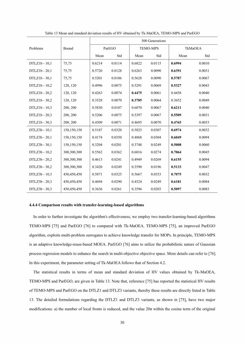
Table 13 Mean and standard deviation results of HV obtained by Tk-MaOEA, TEMO-MPS and ParEGO

500 Generations

Problems Bound ParEGO TEMO-MPS TkMaOEA

Mean Std Mean Std Mean Std

DTLZ1b - 10,1 75,75 0.6214 0.0114 0.6822 0.0115 0.6994 0.0010

DTLZ1b - 20,1 75,75 0.5720 0.0128 0.6263 0.0090 0.6391 0.0031

DTLZ1b - 30,1 75,75 0.5201 0.0106 0.5628 0.0090 0.5787 0.0067

DTLZ1b - 10,2 120, 120 0.4996 0.0075 0.5291 0.0069 0.5327 0.0043

DTLZ1b - 20,2 120, 120 0.4263 0.0074 0.4475 0.0061 0.4458 0.0040

DTLZ1b - 30,2 120, 120 0.3528 0.0070 0.3705 0.0064 0.3652 0.0049

DTLZ1b - 10,3 200, 200 0.5830 0.0107 0.6070 0.0067 0.6211 0.0040

DTLZ1b - 20,3 200, 200 0.5206 0.0075 0.5397 0.0067 0.5509 0.0031

DTLZ1b - 30,3 200, 200 0.4509 0.0071 0.4695 0.0070 0.4765 0.0053

DTLZ3b - 10,1 150,150,150 0.5187 0.0320 0.5825 0.0307 0.6974 0.0032

DTLZ3b - 20,1 150,150,150 0.4174 0.0350 0.4868 0.0304 0.6049 0.0094

DTLZ3b - 30,1 150,150,150 0.3204 0.0201 0.3748 0.0249 0.5008 0.0060

DTLZ3b - 10,2 300,300,300 0.5562 0.0362 0.6016 0.0274 0.7064 0.0045

DTLZ3b - 20,2 300,300,300 0.4613 0.0241 0.4949 0.0269 0.6155 0.0094

DTLZ3b - 30,2 300,300,300 0.3420 0.0249 0.3590 0.0196 0.5133 0.0047

DTLZ3b - 10,3 450,450,450 0.5871 0.0325 0.5667 0.0353 0.7075 0.0032

DTLZ3b - 20,3 450,450,450 0.4694 0.0290 0.4524 0.0249 0.6181 0.0084

DTLZ3b - 30,3 450,450,450 0.3636 0.0261 0.3596 0.0203 0.5097 0.0083

4.4.4 Comparison results with transfer-learning-based algorithms

In order to further investigate the algorithm's effectiveness, we employ two transfer-learning-based algorithms

TEMO-MPS [75] and ParEGO [76] to compared with Tk-MaOEA. TEMO-MPS [75], an improved ParEGO

algorithm, exploits multi-problem surrogates to achieve knowledge transfer for MOPs. In principle, TEMO-MPS

is an adaptive knowledge-reuse-based MOEA. ParEGO [76] aims to utilize the probabilistic nature of Gaussian

process regression models to enhance the search in multi-objective objective space. More details can refer to [76].

In this experiment, the parameter setting of Tk-MaOEA follows that of Section 4.2.

The statistical results in terms of mean and standard deviation of HV values obtained by Tk-MaOEA,

TEMO-MPS and ParEGO, are given in Table 13. Note that, reference [75] has reported the statistical HV results

of TEMO-MPS and ParEGO on the DTLZ1 and DTLZ3 variants, thereby these results are directly listed in Table

13. The detailed formulations regarding the DTLZ1 and DTLZ3 variants, as shown in [75], have two major

modifications: a) the number of local fronts is reduced, and the value 20π within the cosine term of the original

31

DTLZ1 is replaced by 2π, and b) the function is combined with two variables to create a suite of related

optimization tasks. The two test function sets are respectively denoted by DTLZ1b−δ1, δ2 or DTLZ3b−δ1, δ2. It

is clear that the larger difference between δ1 and δ2 means the lower similarity. In this experiment,

δ1 {10,20,30} and δ2 {1,2,3} are set to generate 18 synthetic multimodal DTLZ functions, as shown in Table

13.

From Table 13, it is observed that TkMaOEA shows a performance superiority to other algorithms. For

DTLZ1b, TEMO-MPS obtains the first ranks on DTLZ1b-20, 2 and DTLZ1b-30, 2. In fact, the statistical results

in terms of HV values of Tk-MaOEA are very close to that of TEMO-MPS on DTLZ1b-20, 2 and DTLZ1b-30, 2.

For other test functions, e.g., DTLZ1b-10, 1-3, DTLZ1b-20, 1, 3, DTLZ1b-30, 1, 3, and all DTLZ3b instances,

Tk-MaOEA obtains the first ranks, performing better than TEMO-MPS. This may be due to the fact that

TEMO-MPS aggregates all objective functions into a single objective function, which causes the inaccurate

identification of new candidate solutions during the search. For DTLZ3b, TkMaOEA outperforms ParEGO and

TEMO-MPS on all the test instances. This can be explained that Tk-MaOEA can accelerate the convergence of

solutions by using the transfer matrix, while TEMO-MPS only aggregates the objective values only through a

random vector, resulting in an inaccurate representation for the corresponding solution.

5. Conclusions

In order to alleviate the effect of the curse of dimensionality in MaOPs, this paper develops a novel

evolutionary optimization framework, called Tk-MaOEA, based on transfer learning assisted by Kriging model.

The aim of Tk-MaOEA is to enhance the selection pressure in fitness evaluation in MaOPs. At the global space

optimization level, transfer learning is used to reduce the number of redundant objectives, by the means of the

deliberately designed transfer matrix. At the objective optimization level, Kriging model is incorporated for

each objective to further reduce the optimization complexity during the evolutionary process. In addition, the fast

non-dominated sorting and FCS strategies are incorporated in environmental selection to save and retrieve the

final non-dominated solutions.

The proposed Tk-MaOEA has been experimentally compared with several popular MaOEAs including

NSGA-III, MOEA/D, MOMBII and VaEA on a set of well-defined test benchmarks. Experimental results show

that Tk-MaOEA is significant superior or at least comparable to its compared algorithms in terms of two

commonly used metrics IGD and HV. It should be noted that Tk-MaOEA sometimes encounters the dilemma of

being easily trapped into local many-objective optima on some test problems Accordingly, we do not declare that

Î Î

32

Tk-MaOEA is always superior to other MaOEAs. The strengths and weaknesses of Tk-MaOEA need to be

investigated further, especially according to the specific features of the problems. A comprehensive sensitivity

analysis of the algorithm's parameters, and the research on real-world applications will be highlighted in our

future work.

APPENDIX

The process of transfer learning that aims to reduce the number of objectives, is based on an important

premise that the properties of original objectives should be maintained as much as possible. Thus, the following

definitions are given and the proposed theorems with respects to the transfer matrix are proven mathematically.

Definition 1: for a population matrix P, the transferred matrix Tr can be transformed from P based on the best

individual in P, by using a transfer matrix T, then

(10)

Theorem 1: In Definition 1, the size of matrix Tr should be (N*TN),where N is the number of individuals in

population P, and TN is the number of objectives that has been reduced.

Proof: Considering that the size of matrix P is (N*M), the size of matrix T should be (M*TN). According to

the matrix multiplication in Definition 1, we can get that Tr=PN*M*TM*TN, and the size of Tr is (N*TN).

Therefore, Theorem 1 is proven.

Definition 2: Given an individual ptm in population Pt, , m=1,2,...N, for a column

vector in the transfer matrix, , j=1,2,...N, and an individual trij in the population Tr,

, j=1,2,...N, according to Definition 1, there exists a relation between them as

(11)

Theorem 2: for an individual trij in the population Tr , j=1,2,...N, each set of

coordinates is the map length in direction of the each column vector in transfer matrix .

Proof: In the implementation of matrix multiplication, the row of previous matrix multiplies the column of

the matrix, as depicted in Definition 2. According to the formula related to the inner product (i.e., Eq.(12)) and

the function cos related to the angle between two vectors (i.e., Eq.(13)), if the length of tk is 1, the formula of

inner product (i.e., Eq.(14)) is the map length in the direction of the tk.. Therefore, the Theorem 2 is proven.

Tr P T= *

1 2( , , , )

M

m m m mt t t tp x x x" = !

1 2( , , , )Tj j j Mjt t t t" = !

1 2( , , , )

TN

j j j jt t t ttr y y y" = !

1

1, 2, and 1,2,

,

m mk t k

Mm j mi i t k

i

y p t m N k TN

x t p t=

= * = =

= * =< >å

! !�

1 2( , , , )

TN

j j j jt t t ttr y y y" = !

33

(12)

(13)

(14)

Acknowledgements

This work is supported by National Natural Science Foundation of China under Grant No. 6177021519,

61503373, and 61572123; National Science Foundation for Distinguished Young Scholars of China under Grant

No. 71325002.

References

[1] E. Zitzler and L. Thiele, “Multiobjective evolutionary algorithms: A comparative case study and the strength Pareto

approach,” IEEE Trans. Evol. Comput., vol. 3, no. 4, pp. 257–271, Nov. 1999.

[2] R. Wang, S. Lai, G. Wu, L.Xing, L. Wang, H. Ishibuchide, "Multi-clustering via evolutionary multi-objective

optimization," Information Sciences, 2018, 450,pp.128-140.

[3] Y. Yuan, H. Xu, B. Wang, et al. "Balancing Convergence and Diversity in Decomposition-Based Many-Objective

Optimizers IEEE Trans. Evol. Comput., vol. 20, no. 2, pp.180-198, 2015

[4] J. G. Herrero, A. Berlanga, and J. M. M. Lopez, “Effective evolutionary algorithms for many-specifications attainment:

Application to air traffic control tracking filters,” IEEE Trans. Evol. Comput., vol. 13, no. 1, pp. 151–168, Feb. 2009.

[5] L. Ma, S.Cheng, X. Wang, M.Huang, H. Shen, X. He, Y. Shi, "Cooperative Two-engine Multi-objective Bee Foraging

Algorithm with Reinforcement Learning," Knowledge-Based Systems,133(2017):278-293,2017.

[6] N. Chen, W. Chen, Y. Gong et al. An Evolutionary Algorithm with Double-Level Archives for Multiobjective

Optimization., IEEE Transactions on Cybernetics, 2015, 45(9):1851.

[7] Y. Xiang, Y. Zhou, M. Li, et al. "A Vector Angle-Based Evolutionary Algorithm for Unconstrained Many-Objective

Optimization", IEEE Transactions on Evolutionary Computation, 2017, 21(1):131-152.

[8] L. Ma, K. Hu, Y. Zhu, H. Chen. Cooperative Artificial Bee Colony Algorithm for Multi-objective RFID Network

Planning, Journal of network and computer applications, 42(2014)143-162.

[9] V. Khare, X. Yao, and K. Deb, “Performance scaling of multi-objective evolutionary algorithms,” in Proc. Evol.

Multi-Criterion Optim., Faro, Portugal, 2003, pp. 376–390.

[10] K. Deb, A. Pratap, S. Agarwal, and T. Meyarivan, A fast and elitist multiobjective genetic algorithm: NSGA-II, IEEE

Trans. Evol. Comput., vol. 6, no. 2, pp. 182–197, Apr. 2002.

[11] E. Zitzler, M. Laumanns, and L. Thiele, SPEA2: Improving the strength pareto evolutionary algorithm, in Proc.

EUROGEN 2001: Evolutionary Methods Design Optimization Control Appl. Ind. Problems, Athens, Greece, 2002, pp.

1,

Mm m jt k i i

ip t x t

=

< >= *å

1cos( , )

Mm ji i

m it k m

t k

x tp t

p t=

*=

*

å

1, cos( , )

Mm m j m mt k i i t t k

ip t x t p p t

=

< >= * = *å

34

95–100.

[12] H. Ishibuchi, N. Tsukamoto, and Y. Nojima, “Evolutionary manyobjective optimization: A short review,” in Proc. IEEE

Congr. Evol. Comput., Jun. 2008, pp. 2424–2431.

[13] M. K¨oppen and K. Yoshida, “Substitute distance assignments in NSGAII for handling many-objective optimization

problems,” in Proc. EMO, vol. 4403. 2007, pp. 727–741.

[14] Z. He and G. G. Yen, “Fuzzy-based Pareto optimality for many-objective evolutionary algorithms,” IEEE Trans. Evol.

Comput., vol. 18, no. 2, pp. 269–285, Apr. 2014.

[15] Z. He, G. G. Yen. Many-Objective Evolutionary Algorithm: Objective Space Reduction and Diversity Improvement[J].

IEEE Transactions on Evolutionary Computation, 2016, 20(1):145-160.

[16] H. Sato, H. Aguirre, and K. Tanaka, “Variable space diversity, crossover and mutation in MOEA solving

many-objective knapsack problems,” Ann. Math. Artif. Intell., vol. 68, no. 4, pp. 197–224, 2013.

[17] H. Ishibuchi, Y. Tanigaki, H. Masuda, and Y. Nojima, “Distance-based analysis of crossover operators for

many-objective knapsack problems,” in Proc. Int. Conf. Parallel Prob. Solv. Nat., Ljubljana, Slovenia, 2014, pp.

600–610.

[18] K. Deb and D. Saxena, “On finding Pareto-optimal solutions through dimensionality reduction for certain

large-dimensional multi-objective optimization problems,” Kanpur Genet. Algorithms Lab., Indian Inst. Technol.

Kanpur, Kanpur, India, KanGAL Tech. Rep. 2005011, 2005.

[19] H. Singh, A. Isaacs, and T. Ray, “A Pareto corner search evolutionary algorithm and dimensionality reduction in

many-objective optimization problems,” IEEE Trans. Evol. Comput., vol. 15, no. 4, pp. 539–556, 2011.

[20] Q. Zhang and H. Li, “MOEA/D: A multiobjective evolutionary algorithm based on decomposition,” IEEE Trans. Evol.

Comput., vol. 11, no. 6, pp. 712–731, Dec. 2007.

[21] N. Chen, W. N. Chen, Y. J. Gong, et al. An Evolutionary Algorithm with Double-Level Archives for Multiobjective

Optimization, IEEE Transactions on Cybernetics, 2015, 45(9):1851-1863.

[22] Q. Zhang, W. Liu, E. Tsang, and B. Virginas, “Expensive multiobjective optimization by MOEA/D with Gaussian

process model,” IEEE Trans. Evol. Comput., vol. 14, no. 3, pp. 456–474, Jun. 2010.

[23] E. Zitzler and S. Künzli, “Indicator-based selection in multiobjective search,” in Parallel Problem Solving from

Nature-PPSN VIII. Berlin, Germany: Springer, 2004, pp. 832–842.

[24] N. Beume, B. Naujoks, M. Emmerich, SMS-EMOA: Multiobjective selection based on dominated hypervolume.

European Journal of Operational Research, 2007, 181(3):1653-1669.

[25] Hernandez Gomez R, CoelloCoello C. MOMBI: A new metaheuristic for many-objective optimization based on the R2

indicator. Evolutionary Computation, 2013:2488-2495.

[26] J. Bader, E. Zitzler, HypE: an algorithm for fast hypervolume-based many-objective optimization. Evolutionary

Computation, 2011, 19(1):45-76.

[27] K. Deb, M. Mohan, S. Mishra, Evaluating the ε-domination based multi-objective evolutionary algorithm for a quick

computation of Pareto-optimal solutions, Evol. Comput., vol. 13, no. 4, pp. 501–525, 2005.

[28] K. Ikeda, H. Kita, S. Kobayashi, Failure of Pareto-based MOEAs: does non-dominated really mean near to optimal.

Evolutionary Computation, 2001. Proceedings of the 2001 Congress on. IEEE, 2001:957-962 vol. 2.

[29] H. Sato, H. E. Aguirre, K. Tanaka, Controlling dominance area of solutions and its impact on the performance of

35

MOEAs, in Evolutionary Multi-Criterion Optimization. Berlin, Germany: Springer, 2007, pp. 5–20.

[30] Z. Xiufen, C. Yu, L. Minzhong, et al., A new evolutionary algorithm for solving many-objective optimization problems.

Systems Man & Cybernetics Part B Cybernetics IEEE Transactions on, 2008, 38(5):1402-12.

[31] S. Kukkonen, J. Lampinen, “Ranking-dominance and many-objective optimization,” in Proc. IEEE Congr. Evol.

Comput. (CEC), Singapore, 2007, pp. 3983–3990.

[32] X. Zou, Y. Chen, M. Liu, and L. Kang, “A new evolutionary algorithm for solving many-objective optimization

problems,” IEEE Trans. Syst., Man, Cybern. B, Cybern., vol. 38, no. 5, pp. 1402–1412, Oct. 2008.

[33] S. Yang,, M. Li, X. Liu, J. Zheng, A grid-based evolutionary algorithm for many-objective optimization. Evolutionary

Computation, IEEE Transactions on, 2013. 17(5), pp. 721--736.

[34] S. Kukkonen, J. Lampinen, “Ranking-dominance and many-objective optimization,” in Proc. IEEE Congr. Evol.

Comput. (CEC), Singapore, 2007, pp. 3983–3990.

[35] K. Deb, H. Jain, “An evolutionary many-objective optimization algorithm using reference-point-based nondominated

sorting approach, part I: Solving problems with box constraints,” IEEE Trans. Evol. Comput., vol. 18, no. 4, pp.

577–601, Aug. 2014.

[36] H. Wang, L. Jiao, X. Yao, Two_Arch2: An Improved Two-Archive Algorithm for Many-Objective Optimization. IEEE

Transactions on Evolutionary Computation, 2015, 19(4):524-541.

[37] R. Cheng, Y. Jin, Olhofer M, et al. A Reference Vector Guided Evolutionary Algorithm for Many-Objective

Optimization. IEEE Transactions on Evolutionary Computation, 2016.

[38] H. K. Singh, A. Isaacs, T. Ray, A Pareto Corner Search Evolutionary Algorithm and Dimensionality Reduction in

Many-Objective Optimization Problems. Evolutionary Computation IEEE Transactions on, 2011, 15(4):539-556.

[39] S. Bandyopadhyay, A. Mukherjee, An Algorithm for Many-Objective Optimization With Reduced Objective

Computations: A Study in Differential Evolution. IEEE Transactions on Evolutionary Computation, 2015,

19(3):400-413.

[40] L. Ma, S.Cheng, X. Wang, M.Huang, H. Shen, X. He, Y. Shi. Cooperative Two-engine Multi-objective Bee Foraging

Algorithm with Reinforcement Learning, Knowledge-Based Systems,133(2017):278-293,2017.

[41] D. Brockhoff and E. Zitzler, “Are all objectives necessary? On dimensionality reduction in evolutionary multiobjective

optimization,” in Proc. 9th PPSN, LNCS 4193. 2006, pp. 533–542.

[42] D. Brockhoff and E. Zitzler, “Objective reduction in evolutionary multiobjective optimization: Theory and

applications,” Evol. Comput., vol. 17, no. 2, pp. 135–166, 2009.

[43] A. L. Jaimes, C. A. C. Coello, and D. Chakraborty, “Objective reduction using a feature selection technique,” in Proc.

GECCO, 2008, pp. 673–680.

[44] H. K. Singh, A. Isaacs, and T. Ray, “A Pareto corner search evolutionary algorithm and dimensionality reduction in

many-objective optimization problems,” IEEE Trans. Evol. Comput., vol. 99, no. 4, pp. 1–18, Aug. 2011.

[45] K. Deb and D. K. Saxena, “Searching for Pareto-optimal solutions through dimensionality reduction for certain

large-dimensional multiobjective optimization problems,” in Proc. IEEE CEC, Jul. 2006, pp.3353–3360.

[46] D. Saxena and K. Deb, “Non-linear dimensionality reduction procedures for certain large-dimensional multiobjective

optimization problems: Employing correntropy and a novel maximum variance unfolding,” in Evolutionary

Multi-Criterion Optimization (Lecture Notes in Computer Science, vol. 4403), S. Obayashi, K. Deb, C. Poloni, T.

36

Hiroyasu, and T. Murata, Eds. Berlin/Heidelberg, Germany: Springer, 2007, pp. 772–787.

[47] B. Scholkopf, A. Smola, and K. R. Muller, “Nonlinear component analysis as a kernel eigenvalue problem,” Neural

Comput., vol. 10, no. 5, pp. 1299–1319, 1998.

[48] L. K. Saul, K. Q. Weinberger, J. H. Ham, F. Sha, and D. D. Lee, “Spectral methods for dimensionality reduction,” in

Semisupervised Learning, O. C. B. Schoelkopf and A. Zien, Eds. Cambridge, MA: MIT Press, 2006.

[49] K. Q. Weinberger and L. K. Saul, “Unsupervised learning of image manifolds by semidefinite programming,” Int. J.

Comput. Vis., vol. 70, no. 1, pp. 77–90, 2006.

[50] A.I.J.Forrester and A. J. Keane, “Recent advances in surrogate-based optimization,” Prog. Aerosp. Sci., vol. 45, no. 1,

pp. 50–79, Jan., 2009.

[51] B. Liu, Q. Zhang, and G. G. E. Gielen, “A gaussian process surrogate model assisted evolutionary algorithm for

medium scale expensive optimization problems,” IEEE Trans. Evol. Comput., vol. 18, no. 2, pp. 180–192, Apr. 2014.

[52] S. Das, S. S. Mullick, and P. N. Suganthan, “Recent advances in differential evolution – An updated survey,” Swarm

Evol. Comput., vol. 27, pp. 1–30, Apr. 2016.

[53] P. S. Palar, T. Tsuchiya, and G. T. Parks, “A comparative study of local search within a surrogate-assisted

multi-objective memetic algorithm framework for expensive problems,” Appl. Soft Comput., vol. 43, pp. 1–19, Jun.

2016.

[54] S. C. Horng, S. Y. Lin, "Evolutionary algorithm assisted by surrogate model in the framework of ordinal optimization

and optimal computing budget allocation", Information Sciences, 2013, 233(2):214-229.

[55] S. Huband, P. Hingston, L. Barone, and L. While, “A review of multiobjective test problems and a scalable test problem

toolkit,” IEEE Trans. Evol. Comput., vol. 10, no. 5, pp. 477–506, Oct. 2006.

[56] H. Yu, Y. Tan, J. Zeng, et al. Surrogate-assisted Hierarchical Particle Swarm Optimization, Information Sciences, 2018,

454-455.

[57] G. Venturelli, E. Benini, and Ł. Łaniewski-Wołłk, “A Kriging-assisted multiobjective evolutionary algorithm,” Appl.

Soft Comput., vol. 58, pp. 155–175, Sep. 2017.

[58] H.-J. Park, H.-K. Yeo, S.-Y. Jung, T.-K. Chung, J.-S. Ro, and H.-K. Jung, “A robust multimodal optimization algorithm

based on a sub-division surrogate model and an improved sampling method,” IEEE Trans. Magn., vol. 54, no. 3, Mar.

2018, Art. ID 8201704.

[59] Y. Jin, “Surrogate-assisted evolutionary computation: Recent advances and future challenges,” Swarm Evol. Comput.,

vol. 1, no. 2, pp. 61–70, Jun. 2011.

[60] C. Sun, Y. Jin, R. Cheng, J. Ding, and J. Zeng, “Surrogate-assisted cooperative swarm optimization of high-dimensional

expensive problems,” IEEE Trans. Evol. Comput., vol. 21, no. 4, pp. 644–660, Aug. 2017.

[61] K. Deb and H. Jain, “An evolutionary many-objective optimization algorithm using reference-point-based

nondominated sorting approach, part I: Solving problems with box constraints,” IEEE Trans. Evol. Comput., vol. 18, no.

4, pp. 577–601, Aug. 2014.

[62] R. Cheng, Y. Jin, M. Olhofer, et al. A Reference Vector Guided Evolutionary Algorithm for Many-Objective

Optimization, IEEE Transactions on Evolutionary Computation, 2016, 20(5):773-791.

[63] B. Chen, W. Zeng, Y. Lin, et al., A New Local Search-Based Multiobjective Optimization Algorithm, IEEE

Transactions on Evolutionary Computation, 2014, 19(1):1-1.

37

[64] S. Jeong, Y. Minemura, and S. Obayashi, “Optimization of combustion chamber for diesel engine using Kriging

model,” J. Fluid Sci. Technol., vol. 1, no. 2, pp. 138–146, Dec. 2006.

[65] R. H. Gómez and C. A. C. Coello, “Improved metaheuristic based on the R2 indicator for many-objective

optimization,” in Proc. Genet. Evol. Comput. Conf., Madrid, Spain, 2015, pp. 679–686.

[66] C. A. C. Coello, G. B. Lamont, and D. A. V. Veldhuizen, Evolutionary Algorithms for Solving Multi-Objective

Problems, 2nd ed. New York, NY, USA: Springer, 2007.

[67] H. Ishibuchi, H. Masuda, Y. Tanigaki, and Y. Nojima, “Difficulties in specifying reference points to calculate the

inverted generational distance for many-objective optimization problems,” in Proc. IEEE Symp. Comput. Intell.

Multi-Criteria Decis. Making (MCDM), Orlando, FL, USA, 2014, pp. 170–177.

[68] X. Zhang, Y. Tian, Y. Jin. A Knee Point-Driven Evolutionary Algorithm for Many-Objective Optimization. IEEE

Transactions on Evolutionary Computation, 2015, 19(6):761-776.

[69] W. J. Connover, Practical Nonparametric Statistics, 3rd ed. New York, NY, USA: Wiley, 1999, ch. 5.

[70] K. Deb, L. Thiele, M. Laumanns, and E. Zitzler, “Scalable test problems for evolutionary multi-objective optimization,”

Dept. Comput. Eng. Netw. Lab., ETH Zurich, Zurich, Switzerland, TIK-Tech. Rep. 112, 2001.

[71] Friedman M. A Comparison of Alternative Tests of Significance for the Problem of m Rankings, Annals of

Mathematical Statistics, 1940, 11(1):86-92.

[72] A. Toffolo, E. Benini, Genetic diversity as an objective in multi-objectiveevolutionary algorithms, Evol. Comput. 11 (2)

(2003) 151–157.

[73] G. Venturelli, E. Benini, Ł. Łaniewski-Wołłk, A Kriging-assisted Multiobjective Evolutionary Algorithm, Applied Soft

Computing, 58(2017): 155-175.

[74] Chugh T, Jin Y, Miettinen K, et al. A Surrogate-Assisted Reference Vector Guided Evolutionary Algorithm for

Computationally Expensive Many-Objective Optimization[J]. IEEE Transactions on Evolutionary Computation, 2018,

22(1):129-142.

[75] Min A T W, Ong Y S, Gupta A, et al. Multi-Problem Surrogates: Transfer Evolutionary Multiobjective Optimization of

Computationally Expensive Problems[J]. IEEE Transactions on Evolutionary Computation, 2017, PP(99):1-1.

[76] Knowles J. ParEGO: a hybrid algorithm with on-line landscape approximation for expensive multiobjective

optimization problems[J]. IEEE Transactions on Evolutionary Computation, 2006, 10(1):50-66.