A novel improved model for building energy consumption prediction basedon model integrationRan Wanga,b, Shilei Lua,b,⁎, Wei Fengb

a School of Environment Science and Engineering, Tianjin University, 92 Weijin Road, Tianjin 300072, Chinab Lawrence Berkeley National Laboratory, Berkeley, CA 94720, USA

A B S T R A C T

Building energy consumption prediction plays an irreplaceable role in energy planning, management, andconservation. Constantly improving the performance of prediction models is the key to ensuring the efficientoperation of energy systems. Moreover, accuracy is no longer the only factor in revealing model performance, itis more important to evaluate the model from multiple perspectives, considering the characteristics of en-gineering applications. Based on the idea of model integration, this paper proposes a novel improved integrationmodel (stacking model) that can be used to forecast building energy consumption. The stacking model combinesadvantages of various base prediction algorithms and forms them into “meta-features” to ensure that the finalmodel can observe datasets from different spatial and structural angles. Two cases are used to demonstratepractical engineering applications of the stacking model. A comparative analysis is performed to evaluate theprediction performance of the stacking model in contrast with existing well-known prediction models includingRandom Forest, Gradient Boosted Decision Tree, Extreme Gradient Boosting, Support Vector Machine, and K-Nearest Neighbor. The results indicate that the stacking method achieves better performance than other models,regarding accuracy (improvement of 9.5%–31.6% for Case A and 16.2%–49.4% for Case B), generalization(improvement of 6.7%–29.5% for Case A and 7.1%-34.6% for Case B), and robustness (improvement of1.5%–34.1% for Case A and 1.8%–19.3% for Case B). The proposed model enriches the diversity of algorithmlibraries of empirical models.

1. Introduction

The building and construction sector together are responsible for36% of global final energy consumption and nearly 40% of total directand indirect carbon dioxide emissions [1]. Building energy savings canbe achieved by improving the building’s dynamic energy performancein terms of sustainable construction management in urban-based builtenvironments [2]. Meanwhile, building operations are information-in-tensive, due to the popularity of smart sensors and the adoption of

intelligent building management systems [3]. A large amount ofbuilding operational data has been recorded to provide a basis forbuilding performance analysis. Therefore, a promising strategy to ad-dress energy savings is to develop big data-driven approaches tobuilding smart energy management.

Prediction models for building management systems have raisedconcerns. The predicted targets are mainly building energy consump-tion (building internal heat gains [4], building cooling loads [5], dis-trict heating load [6], electricity demand [7], peak power demand [8]),

⁎ Corresponding author at: School of Environment Science and Engineering, Tianjin University, 92 Weijin Road, Tianjin 300072, China.E-mail address: lvshilei@tju.edu.cn (S. Lu).

T

indoor temperature (commercial buildings [9] and residential buildings[10]), thermal sensation votes [11], and system or unit performanceindicators [12]. The service objectives of prediction models in the en-ergy management system mainly include optimized control [13] andfault detection [14]. Optimized control includes matching the supplyand demand of building energy [15], maintaining the indoor thermalcomfort [9], and operating the unit and system in an optimal state(HVAC systems [16], energy recovery systems [17], and radiant floorsystems [18]). With the support of sufficient training data, fault de-tection helps to distinguish whether the patterns of monitoring data aresimilar to those of the normal training data [19]. Hence, improving theaccuracy, robustness, and generalization performance of the predictionalgorithm is key to ensure efficient building operations [20].

The data-driven model has become the most popular method used inthe field of building energy due to its low time consumption and goodprediction performance [21]. Commonly used data-driven models canbe classified as single prediction models, integration prediction models,and improved prediction models.

The single prediction model, which is the type of most traditionalmodels, has single algorithm architectures such as support vector re-gression (SVR) [22], artificial neural network (ANN) [23], and multiplelinear regression models (MLR) [24].

In contrast, integration prediction models integrate single predic-tion algorithms into a more accurate model by combining strategies,which can be divided into various types in view of the order betweenbase models (in parallel or in series) and whether base models are thesame kind of algorithms (homogeneous or heterogeneous integration)[25]. For example, the Random Forest (RF) model is a parallel homo-geneous integration model, while Gradient Boosted Decision Tree(GBDT) and Extreme Gradient Boosting (XGBoost) models are serieshomogeneous integration models.

Improved prediction models use auxiliary algorithms or frameworksto make up for the deficiencies of the original prediction algorithm.There are generally three forms: (1) the pre-assisted algorithm, whichimproves the data quality to make up for the specific requirements ofthe prediction algorithm [26]; (2) the assisted optimization algorithm,which is used to perform hyperparameter tuning of a prediction algo-rithm [27]; and (3) nesting of an auxiliary improvement framework onthe base prediction algorithm, to improve model performance [7]. Mostof the existing research is based on single or integration models, whichlack improvements in the essence of the algorithm. However, the im-proved prediction model can enrich the algorithm library and con-tinuously improve the overall accuracy level of building energy fore-casting, which is crucial for scheduling and managing energy usage[15]. Therefore, it is quite important to develop improved prediction

models.This paper proposes a novel prediction method for building energy

prediction based on the principle of algorithm integration. The methodis applied to two actual cases as a demonstration, and the results verifyits reliability in short-term building energy prediction. Moreover, themethod is compared with some state-of-the-art or popular predictionmethods from the perspectives of robustness, accuracy, and general-ization performance, and its superiority is verified. The proposedmethod enriches the library of energy consumption prediction models.Hence, this study has a unique significance.

2. Literature review

The most important two modules for the prediction model aremodel inputs and prediction algorithms. The model inputs sectionmainly summarizes the input types found in existing research and looksforward to the development trend. The prediction algorithm is sum-marized from three algorithm types: single prediction, integrationprediction, and improved prediction. The literature related to the al-gorithms’ performance comparison and performance evaluation di-mensions is also reviewed.

2.1. Selection of model inputs

Input data can be classified into meteorological data, occupancydata, historical data, and time type information. Meteorological dataare relatively easy to obtain by means of weather stations. Occupancydata mainly affects the building energy consumption by changing theenergy supply status, which refers to human behaviors and buildingusage schedules. Due to the great uncertainty and high requirements forthe monitoring system, few studies have directly taken occupancy dataas input data for the prediction model; according to the literature, theproportion of meteorological and occupancy data used in related re-search articles is 60% and 29%, respectively [25]. In addition, someresearchers utilized time type information (e.g., time of the day, day ofthe week, day type) to remedy the information lost from the omission ofoccupancy data [28]. Historical data such as historical energy is apopular input because it indicates the trend of the load profile in amathematical way. The model inputs in most studies generally involvea combination of two or more of these types.

For example, meteorological data and historical energy consump-tion were used for daily building electricity forecasting [29]. Onlyhistorical energy consumption was used in yearly building electricityforecasting [30] and daily building electricity forecasting [31]. Me-teorological data and day type were used in hourly electricity

Nomenclature

Abbreviation

AI Artificial intelligenceRMSE Root mean squared errorMAE Mean absolute errorMAPE Mean absolute percentage errorCVRMSE Coefficient of variation of the root mean square errorR2 Coefficient of determinationx Inputy OutputP Output of the train set of the base modelT Output of the test set of the base model

Method

RF Random forest

SVR Support vector regressionkNN k Nearest NeighborsGBDT Gradient boosting decision treeXGBoost Extreme gradient boostingANN Artificial neural networkMLR Multiple linear regressionARIMA Autoregressive integrated and moving averageBPNN Back-propagation neutral networkGRNN Generalized regression neural networkRBFNN Radial basis function neural networkOLS Ordinary least squaresMARS Multivariate adaptive regression splinesGPR Gaussian process regressionES Exponential Smoothing

based on SVR and ANN [52]. Chae et al. constructed an integrationmodel based on three ANN algorithms and applied it to predict sub-hourly electricity usage in commercial buildings [28]. In contrast,homogeneous models are constructed by the same single models ondifferent training sets. RF has been effectively applied to peak powerdemand [8], electricity load forecasting [53], and heating and coolingloads [54]. In recent years, GBDT and XGBoost have also graduallybeen applied in the field of building energy. The GBDT model exhibitsthe highest performance in the prediction of energy consumption byappliances in a low-energy house [55], electricity load forecasting forutility energy management systems [56], and electricity load fore-casting for utility energy management systems [57]. The XGBoostmodel has been used to construct a prediction model for early detectionof faults in HVAC systems [58] and building energy performancegrading [59]. In general, integrated algorithms are becoming increas-ingly popular in the field of energy prediction.

2.2.3. Improved prediction modelsSome studies have focused on the improved prediction model to

achieve better accuracy.Auxiliary algorithms can be applied to improve data quality before

the prediction algorithm is established. For example, Ding et al. used K-means and hierarchical clustering methods to classify input variables toimprove prediction accuracy [60]. Yuan et al. proposed a sample dataselection method based on a grey correlation method integrated with anentropy weight method; the result demonstrated that the accuracy ofBPNN had improved [26]. Ding et al. divided the sample data by ten-fold cross-validation to improve the accuracy of the SVR model in short-term and ultra-short-term predictions of cooling load [61]. A hybridSVR was applied to predict the hourly electric demand intensity; themulti-resolution wavelet decomposition was introduced to divide theinitial series into several parts, to alleviate the interferential influenceon modeling [62].

Optimization algorithms can be used for hyperparameter tuning toimprove base model performance. For example, Li et al. applied animproved particle swarm optimization algorithm to adjust the structureweights and threshold values of ANN [63]. Zhong et al. proposed anovel vector field-based SVR method, which improves the performanceof SVR, including accuracy, robustness, and generalization capabilitiesthrough multi-distortions in the sample data space or high-dimensionalfeature space mapped by a vector field to find the optimal feature space[15]. An evolutionary-based ANN algorithm has been proposed forshort-term load forecast of electricity, and optimal network parametersare found to reduce the forecasting error [27].

Some integration strategies and frameworks can be used to improvethe structure of the base algorithm to enhance its performance. Forexample, Fan et al. exploited the potential of deep learning and com-pared its performance in cooling load prediction with typical featureextraction methods and popular prediction techniques in the buildingfield. Results showed that deep learning can enhance the predictiveperformance, especially when used in an unsupervised manner [64].Jatin et al. proposed a Long Short Term Memory based deep learningframework to forecast electricity demand by taking care of long-termhistorical dependencies, and proved the method’s effectiveness bycomparing it with ANN and SVR [7]. Alessandro et al. proposed aBayesian deep learning-based method to predict electricity price, andproved the method’s robustness in out-of-sample conditions [65]. Onthe whole, improved prediction models enrich the algorithm library ofthe prediction model and promote the accuracy of the energy predictionfield overall.

2.3. Comparison of prediction models

From the perspective of algorithm types, existing studies comparethe same, as well as different, types of models.

Many studies have conducted comparisons between the same type

forecasting [32] and sub-hourly electricity forecasting [33]. Meteor-ological data and occupancy schedules were used in the prediction of heating/cooling consumption for a solar house [34]. Few studies used other variables as inputs; for example, indoor environmental factors (temperature and relative humidity) and meteorological data were used together to predict building cooling energy consumption [15]. Other than meteorological data, occupancy and hour-type/day-type pre-treated air unit operation schedule were used for cooling load predic-tion [35].

Most researchers collected input data based on their knowledge of the prediction model and data availability [25]. Whether it is in the establishment of the model or the actual maintenance of the model later, collection of meteorological data is relatively easy. Additionally, day types and historical data are deterministic prior information; so the use of these three types of data is still dominant. Meanwhile, the number of inputs for each input data type has increased as modeling techniques have developed [5]. For example, meteorological data were only related to outdoor temperature in early studies [36], but this gradually expanded to outdoor temperature, relative humidity, and solar radiation [37]. Currently, wind speed and wind direction also serve as indicators [15].

2.2. Evolving prediction models

2.2.1. Single prediction modelsThe single prediction model’s main feature is that it consists of only

the base prediction algorithm. Early research related to building energy predictions generally involves single prediction models, which are mainly divided into statistical and artificial i ntelligence m odels [38]. Statistical models are an established, simple tool for long-term predic-tion [39]. MLR, Exponential Smoothing (ES), and auto-regressive in-tegrated and moving average (ARI MA) models are popular statistical approaches that are applied in the prediction model. The MLR model was used to forecast the daily peak load [40] and monthly electricity demand [41]. The ES model was used for hourly load forecasting, with a lead time of 1–24 h [42]. The ARI MA model was used to predict hourly electricity load and daily peak load [43]. The kNN is also a simple and effective s tatistical m odel, w idely a pplied t o w ind speed forecasting [44], electricity forecasting [45], and solar power fore-casting [46].

Due to high accuracy, artificial i ntelligence ( AI ) a lgorithms are widely used; the transition from statistical to AI methods occurred around 1991 to 2001 [39]. The SVR and the ANN series of algorithms are commonly used predictive models [47]. SVR is based on the structural risk minimization principle, which performs well in time series and non-linear prediction [48]. I t was first u sed i n t he fi eld of building energy consumption forecasting in 2005 [49]. ANN is a non-linear statistical learning technique inspired by biological neural net-works, applied to various types of building energy consumption fore-casts, such as overall building energy consumption, cooling and heating loads, and electricity consumption. Back-propagation neural network (BPNN) and Generalized regression neural network (GRNN) are two representative types of ANN. Ben et al. used GRNN to predict the cooling load [36]. Ekici et al. proved the reliability and accuracy of BPNN in building heating load forecast [50].

2.2.2. Integration prediction modelsA more advanced data-driven method called integration learning

was introduced in the early 1990s. I ntegration learning is also called fusion learning, aggregation, combination, ensemble, and other names [25]. An integration model is defined as a framework that combines the advantages of multiple single models to improve overall performance. It is divided into two types: heterogeneous and homogeneous. Hetero-geneous models use the same dataset to construct single models by training different a lgorithms o r t he s ame a lgorithm w ith different parameter settings [51]. Chou et al. constructed an integration model

models included linear regression with ordinary least squares (OLS),RF, SVR, multivariate adaptive regression splines (MARS), Gaussianprocess regression (GPR), and ANN. The comparison shows that GPRproduced the best precision and robustness, and was easy to implement,but it became inefficient for large training sets compared to ANN andMARS [74]. Both studies have shown there was no consensus on a“best” model after considering all their performances. Zhong et al.verified the performance of an improved SVR algorithm from threeaspects of prediction accuracy, generalization ability, and robustness bycomparing it with commonly used data-driven models and state-of-the-art models [15]. Cai et al. compared two deep neural network modelswith the Seasonal ARIMA model for accuracy, computational efficiency,generalizability, and robustness [20]. Fan et al. investigated and com-pared the usefulness of advanced recurrent neural network-basedstrategies for building energy predictions in terms of prediction accu-racy and computation load [75].

2.4. A summary of the previous research

Most studies have established prediction models using base datamining algorithms. Among them, the traditional single predictionmodel is the most widely used because of the simple algorithm in-volved. The integrated model is becoming increasingly popular forbuilding energy use prediction due to its remarkably improved pre-diction accuracy [25]. The integrated model uses multiple base modelsto predict the results, and the diversity among these base models willreduce the prediction error of the overall system. In terms of buildingenergy consumption prediction, the accuracy improvement of the in-tegrated model in the reviewed research can be up to 50% based on theMAPE index [8] and up to 4.9% based on the RMSE index [71].

Improved algorithms can effectively improve the accuracy of pre-diction models; however, related research is rarely compared with basicdata-mining algorithms. Therefore, it is of great significance to proposean improved prediction model with better performance for enrichingthe empirical model library of energy consumption prediction.

The horizontal comparison between different models can be con-ducive to the intuitive display of relative advantages and disadvantages,and most of the current research has evaluated models based solely onaccuracy. Moreover, from the perspective of practical engineering ap-plications, the model performance should be evaluated from multipleperspectives, including accuracy, generalization, and robustness, in

Fig. 1. The research framework.

of model. For example, Li et al. compared SVR with several ANN models for predicting hourly building cooling load [66]. Massana et al. used SVR, MLR, and ANN to predict short-term load for non-residential buildings [67]. Wang et al. compared SVR and three ANN models (BPNN, radial basis function neural network [RBFNN], and GRNN) for predicting hourly residential electricity use [68]. These studies have shown that SVR improved building energy use prediction better than other AI-based prediction methods. ANN was compared with regression models for annual urban residential buildings’ energy consumption [69] and HVAC hot water energy consumption [70]; both studies in-dicated that ANN could perform better than regression methods for short-term forecasting. Comparisons have also been made between single and integrated models. For example, three neural network models and their integrated forms were used for heating consumption prediction, and the results showed that the integrated model has better prediction accuracy [71]. Ahmad et al. compared ANN and RF models for predicting the hourly HVAC energy consumption of a hotel, and ANN performed with marginally better precision than RF, but RF has an advantage in processing multi-dimensional complex data due to its ease of tuning and modeling [72]. RF was compared with RT and SVR to validate its superiority in building energy prediction [53]. One example of a comparison between a single model, integrated model, and hybrid model is the study by Zhong et al., which compared an improved SVR algorithm with the MLR, BPNN, SVR, deep learning, and GBDT models [15].

I t is important to note that most prior research studies have only compared model performance in terms of precision, although a small number of research studies have compared model performance from multiple perspectives. For example, SVR and three ANN models (in-cluding BPNN, RBFNN, and GRNN) were applied to hourly cooling load forecasting of an office building; the result demonstrated that the SVR and GRNN could achieve better accuracy and generalization than the BPNN and RBFNN [66]. Wang et al. compared five models (SVR, ANN, RF, GBDT, and XGBoost) with respect to interpretability, accuracy, robustness, and computational efficiency wh en ap plied to hourly heating energy consumption. BPNN exhibited the lowest precision, ef-ficiency, robustness, and interpretability, while RF showed the highest overall performance, with the highest accuracy, robustness, and inter-pretability. However, RF efficiency wa s le ss th an th e XG Boost model [73]. Ostergard et al. compared six prediction models with respect to accuracy, efficiency, ease-of-use, robustness, and interpretability. These

3. Framework and methodologies

This study seeks to contribute to the existing state of the art byfocusing on the following:

• This paper proposes a novel improved prediction algorithm. Its coreis to build an integration framework and apply it to the basic modelsto improve overall prediction performance. The improved predic-tion model includes two main features: it enables comprehensivedata observation and reduces overfitting. Based on the character-istics of different prediction algorithms, it can observe sample datafrom different spatial and structural perspectives. This study com-bines the observations of various base models into the form of“meta-features” to enable the overall model to more comprehen-sively observe the sample data. And this method reduces overfittingby distorting the sample data space.

• The superiority of the proposed model is verified by several state-of-the-art or popular prediction models. Model performance is eval-uated from three dimensions: accuracy, generalization, and robust-ness.

3.1. Research framework

This study is dedicated to obtaining a novel method of high preci-sion, high robustness, and high generalization capabilities for buildingenergy prediction. Subsequently, the proposed method is applied to areal case to establish a prediction model and verify its effectiveness.This section focuses on the construction of the novel model and caseintroduction. The research framework is shown in Fig. 1.

3.2. Proposed method

3.2.1. Algorithm frameworkBased on the idea of model fusion, this paper presents a new energy

consumption prediction model. Single models can observe data in dif-ferent spatial and structures angles, the proposed model (called thestacking model hereafter) can synthesize the observations of all singlemodels to achieve an improved prediction performance by constructing

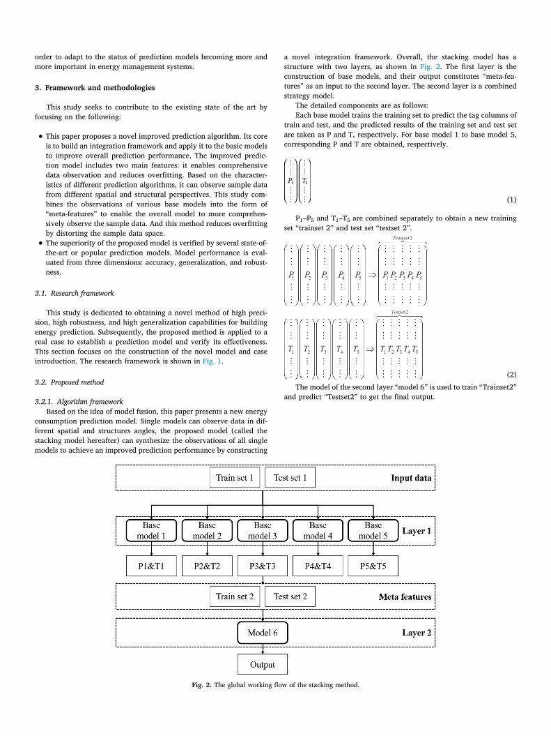
a novel integration framework. Overall, the stacking model has astructure with two layers, as shown in Fig. 2. The first layer is theconstruction of base models, and their output constitutes “meta-fea-tures” as an input to the second layer. The second layer is a combinedstrategy model.

The detailed components are as follows:Each base model trains the training set to predict the tag columns of

train and test, and the predicted results of the training set and test setare taken as P and T, respectively. For base model 1 to base model 5,corresponding P and T are obtained, respectively.

P T1 1

(1)

P1–P5 and T1–T5 are combined separately to obtain a new trainingset “trainset 2” and test set “testset 2”.

(2)

The model of the second layer “model 6” is used to train “Trainset2”and predict “Testset2” to get the final output.

Fig. 2. The global working flow of the stacking method.

order to adapt to the status of prediction models becoming more and more important in energy management systems.

(3)

3.2.2. Construction of base modelsIn order to avoid overfitting, fivefold cross-validation is used for

each base model. As shown in Fig. 3, divide “trainingset 1” into fivenon-intersecting sets and mark them as traina to traine. Assume that thetraining set is a matrix of M rows and N columns. The matrix of the fivetrain sets is as shown in Eq. (4).

(4)

Taking base model 1 as an example, base model 1 is trained by thecombination of traina–traind to build Modele. And the dataset traine ispredicted by Modele to obtain Prede as shown in Eq. (5).

Similarly, Modela–Modeld are built, and Preda–Predd are obtained byusing traina, trainb, trainc, and traind as prediction sets, respectively.

(6)

Finally, Preda–Prede is combined to form P1.

+ + + + = =Pred Pred Pred Pred Pred

PredPredPredPredPred

Pa b c d e

a

b

c

d

e

1

(7)

Using the established Modela–Modele to predict the testset to getTesta–Teste separately, and finally average the five results to get T1.

(8)

+ + + + =Test Test Test Test Test P( )/5a b c d e 1

(9)

3.2.3. The selection of base modelsThese base models are selected based on two principles: popularity

and diversity. First, all the selected algorithms should have been widelyused in solving complex modeling and prediction problems, and studiesshould have proven their performance to be encouraging. Second, themaximized integration diversity will make the integration results morerobust and more accurate [8], and it is best to “cross the space” betweenthe selected base models. That means algorithms with large differences

in principle should be selected. Therefore, this study selects five com-monly used models (RF, kNN, SVR, GBDT, and XGBoost) as basemodels. These differ in their non-linearity handling abilities, modelarchitectures, and inference mechanisms.

The RF model was developed by Breiman in 2001 for both

Fig. 3. The construction of the base model (Taking Base model 1 as an example).

(5)

The detailed calculation formula is shown in [82].

3.3. Model performance evaluation

3.3.1. AccuracyTo ensure the reliability of the evaluation results, a variety of ac-

curacy metrics can be used, including mean absolute error (MAE), rootmean squared error (RMSE), mean absolute percentage error (MAPE),and the coefficient of variation of root mean square error (CVRMSE).Each of these indicators has a different emphasis. MAE is based onabsolute error, which can visually show the average distance betweenthe predicted value and the actual value. RMSE is used to identify largeerrors and evaluate the fluctuation of model response regarding var-iance. The metric punishes large errors severely because it geome-trically amplifies the error [53]. MAPE expresses accuracy in percen-tage and reduces the effect of absolute errors caused by individualoutliers. CVRMSE normalizes the prediction error and can provide aunitless metric that is more convenient to compare [38]. For all fourindicators, the smaller the value, the better the model performance. Inthis article, four indicators are used in conjunction with each other.MAE is mainly used to show the difference between absolute errors,RMSE is used to identify large errors, and MAPE and CVRMSE aremainly used to compare the accuracy differences between differentmodels.

= ×=CVRMSEy y

y

( )

¯100%

ni

n

i i1

1

2

(10)

==

RMSEn

y y1 ( )i

n

i i1

2

(11)

= ×=

MAPEn

y yy

1 100%i

ni i

i1 (12)

==

MAEn

y y1 | |i

n

i i1 (13)

where yi, yi , and y represent the actual value, the predicted value, andthe average actual value, respectively.

3.3.2. GeneralizationGeneralization performance refers to the model’s ability to predict

samples beyond the training range.

Fig. 4. Exterior view of the case buildings: (a) Case A; (b) Case B.

classification and regression problems [76]. It consists of many decision regression trees but is not a simple average of the predictions of all decision trees. I ts four features are bootstrap resampling, random fea-ture selection, out-of-bag error estimation, and full-depth decision tree growing. Repeated sampling of the original datasets generates each of the regression trees. The samples of about one-third are not extracted at each repeated sampling, which forms a control dataset. RF is not easy to overfit and has good noise immunity [77].

The kNN model is a non-parametric learning algorithm used for either classification o r r egression. k NN r egression u ses t he averaging method, which is the average output of the most recent K samples, as the regression prediction. I t is non-parametric, as it does not learn an explicit mapping relationship between inputs and outputs. The para-meter k, which defines t he n umber o f c onsidered n eighboring ob-servations, is important for model performance. The larger the k value, the better the generalization ability of the model, but it is easy to fit; the smaller the k value, the better the fitting effect of th e model, bu t the generalization ability is not enough. kNN is regarded as one of the simplest learning algorithms [78].

The concept of the SVR model derives from the computation of a linear regression function in a high-dimensional feature space, where the input data are mapped through a non-linear function [79]. The most prominent advantage of SVR is the uniqueness and global optimality of the generated solution, as it does not require non-linear optimization with the risk of sucking in a local minimum limit. The Gaussian radial basis function is adopted as the kernel function because it can map the low-dimensional input space into the high-dimensional space, and only one parameter needs to be set [37].

GBDT is also called multiple additive regression trees (MART) or gradient boosting machine (GBM), and it is an iterative decision tree algorithm [80]. I ts implementation logic is to build the weak learner (regression tree) in turn and try to reduce the deviation of the com-biner. GBDT, based on numerical optimization, uses the fastest descent method to solve the optimal solution of loss function; fitting t he ne-gative gradient using the regression tree and calculating the step length using the Newton method. This makes it possible to reduce the loss function as fast as possible for each training and converge to the local optimal or global optimal solution as quickly as possible [81].

XGBoost is an improved algorithm based on the GBDT algorithm. It has the following improvements: First, XGBoost is based on analytic thinking. The loss function is expanded to the second-order derivatives to obtain the analytic solution as the gain to establish trees so that the loss function is optimal. Second, XGBoost adds regular terms to control model complexity. From the point of bias-variance trade-off, the regular terms reduce the model’s variance and prevent overfitting. Third, XGBoost supports parallel learning and is relatively faster in computing.

70% and 30%, respectively. The training set can be used to constructthe prediction model, and the test set, which contains values outside thetraining set, can be used to examine the generalization ability.Prediction models were implemented in the Python environment (Ver.3.6). The base model of the first layer is RF, XGBoost, GBDT, SVR, andkNN, and the combined model of the second layer is GBDT. The mainparameters affecting the RF model include the maximum depth of thetree (MD), the number of trees (NT), and the maximum of features(MF). Compared to the RF model, the GBDT model includes the hy-perparameter of the learning rate (LR) as well. When constructing atree, XGBoost can subsample the original datasets. Unlike RF, thesample here is not placed back. The hyperparameters that affect theXGBoost model are mainly MD, NT, LR, and subsample. The SVR modelhas two crucial parameters: c and γ. The c is the penalty factor, which isthe tolerance for the error. The γ is the coefficient of the kernel func-tion, which implicitly determines the distribution of the data aftermapping to the new feature space [73]. The k and the p of the Min-kowski distance formula are the main hyperparameters affecting thekNN model [78]. To intuitively prove the improvement effect of theimproved algorithm, the prediction results of base models also outputseparately. The base models in the stacking model were tuned in turn,and their optimized hyperparameters are summarized in Table 3.

5. Results and discussion

5.1. Model accuracy

Fig. 7 shows fitting results between the predicted and the corre-sponding measured value for each prediction model. The scatter ofmeasured data—predicted data—is distributed on the sides of thebaseline. Furthermore, the stacking model fits better than the othermodels, with R2 equal to 0.86 and 0.92 for cases A and B, respectively.The R2 of RF, GBDT, SVR, XGBoost, and kNN are 0.79, 0.82, 0.79, 0.82,and 0.84, respectively, for Case A, and 0.73, 0.85, 0.9, 0.89, 0.96, re-spectively, for Case B. Fig. 8 shows the relative error distribution of allmodels for the two cases. When based on the mean relative error, thestacking method achieves higher accuracy than all the other fivemodels, with accuracy improvement being about 9.5%–31.6% for CaseA and 16.2%–49.4% for Case B. The x-axis is the heating load, so it canvisually show the variation of the relative error with the heating loadlevel. As shown, the error of the stacking model is not the smallestcompared to other models when the heating load was relatively low,but the error is smallest when the heating load is in the middle position.The pattern of actual heating loads is considered to be a normal dis-tribution with the characteristics of “more in the middle and less at bothends” (as shown in Fig. 9). Therefore, from the perspective of en-gineering practice, the stacking model has better practicability in termsof cumulative error. Table 4 summarizes four error metrics of eachmodel calculated using Eqs. (10)–(13). For the stacking model, theCVRMSE, RMSE, MAE, and MAPE are 10.60%, 23.53, 16.14 and 7.66%,respectively, for Case A, and 8.96%, 13.81, 10.61, and 7.51%,

Table 1Basic information on the case study buildings.

Items Case A Case B

Size (m2) 10,762.0 12,236.2Insulation type Self-insulation External insulation

Shape Coefficient 0.18 0.22Window-wall ratio South 0.34 0.53

East 0.13 0.29West 0.15 0.42North 0.43 0.37

U-value (W/(m2⋅K)) Roof 0.17 0.55External wall 0.46 0.55

External window 2.5 2.5

3.3.3. RobustnessIn the field of machine learning, robustness is defined as the ability

of the model to resist external environmental disturbances to ensure the stability of its working performance. For building energy, there are many reasons why the collected operational data may deviate from reality, such as monitoring system failure, instrument damage, sudden stopping of the unit, and so on. Additionally, in the actual operation of the prediction model, weather forecasting is generally used to obtain meteorological data, but the error in weather forecasting will affect the model performance. Many studies have used the method of adding different intensities of noise to the testing data to measure the model’s robustness. For example, Gaussian white noise was used to con-tinuously enhance noise intensity [20]. R2 reflects the proportion of the total variation of the dependent variable that can be explained by the independent variable. Therefore, it can be used as the main indicator of the model’s robustness.

4. Case studies

4.1. Building information

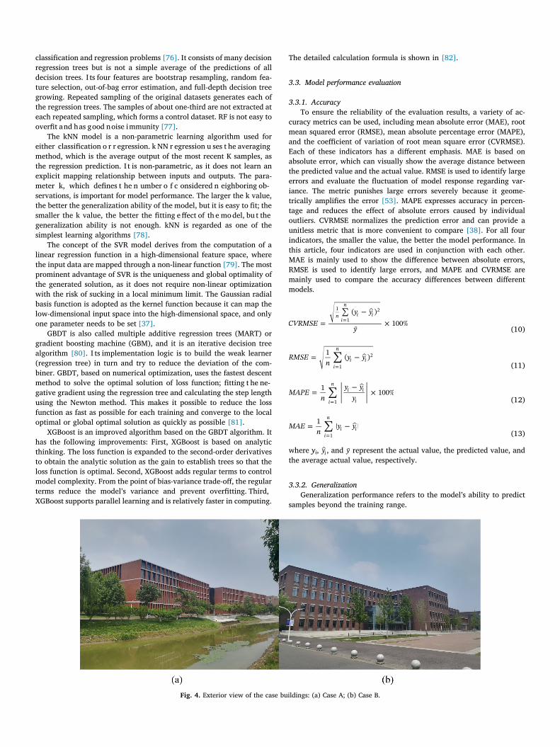
Operation data retrieved from two educational buildings in the coastal city of Tianjin, China, is employed for the case study. The case study buildings mainly contain classrooms for students and offices for university staff. Case A is a three-star green building with three stories, and Case B is a conventional building with four stories. Their elevations are shown in Fig. 4. Table 1 summarizes the basic information of the case study buildings, including shape coefficient, insulation level of the envelope, and window-to-wall ratio. The insulation level of Case A is much better than that of Case B. Both buildings use district heating to maintain an indoor thermal environment during winter, and the heating energy is supplied by the energy station in the school.

4.2. Input data and data collection

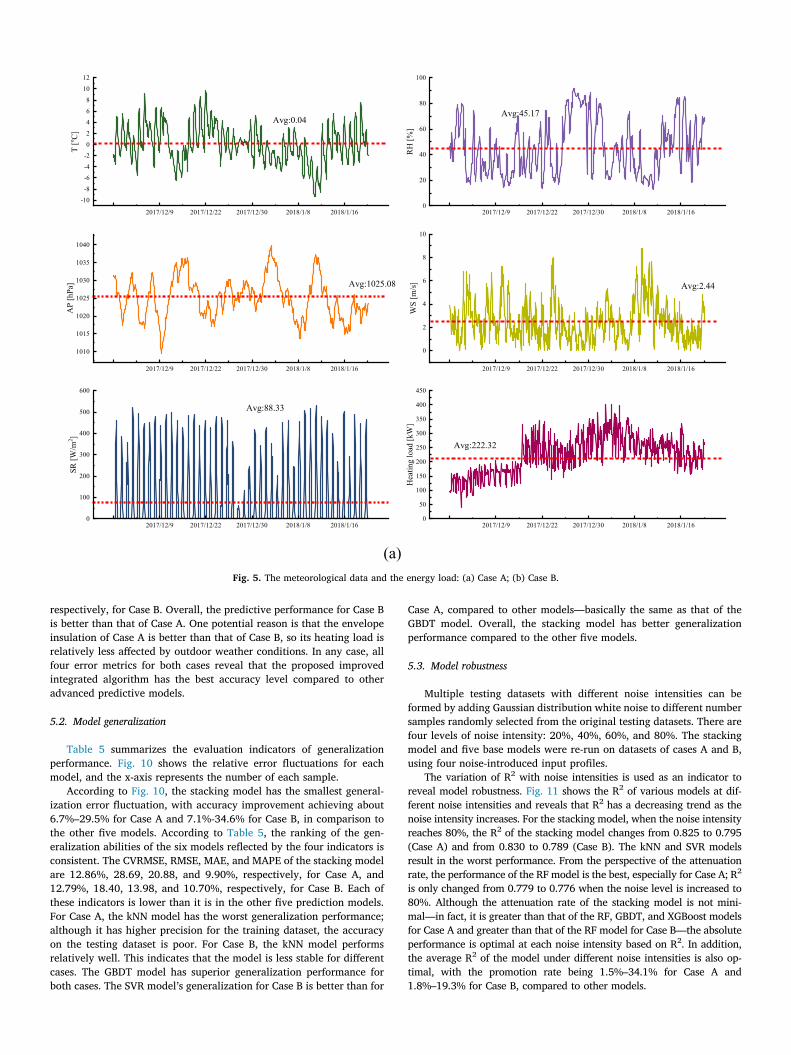
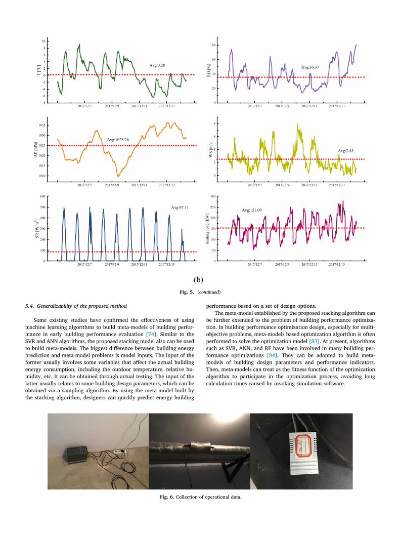
The input variables can be divided into three general categories: (1) meteorological data (including outdoor dry bulb temperature, wet bulb temperature, relative humidity, wind direction, wind speed, air pres-sure, horizontal total radiation), (2) time variable (hour of the day, day type), and (3) historical data (energy consumption at the same time as the previous day). We conducted an on-site collection of the actual operational data, and obtained integrated datasets of Case A ranging from Dec. 1, 2017 to Jan. 20, 2018, with a time interval of 1 h, and Case B ranging from Dec. 5, 2017 to Dec. 14, 2017, with a time interval of 0.5 h. Fig. 5 shows the meteorological data and heating load data for the two buildings.

The total building heating load can be calculated based on the water flow rate, the supply, and the return water temperature. A portable flow meter was installed on the return manifold at the thermal inlet of each case building. The two probes of the wall-mounted dual-temperature self-recording instrument were placed inside the insulation layer of the water supply and return pipes. Fig. 6 shows the field test, and Table 2 shows the instrument parameters such as measurement accuracy.

Meteorological data were obtained from an on-campus weather station located approximately 100 m from the test building. The weather station consists of a complete set of weather sensors, including temperature, humidity, wind speed, wind direction, rainfall, and solar intensity. Table 2 shows their measurement accuracy.

4.3. Model implementation

The operational data in the previous section has revealed that there are differences in the energy use characteristics of the two case build-ings; so we can apply the prediction algorithm to each building sepa-rately to verify the method scalability. For each case, the entire dataset can be divided into training and testing datasets, with proportions of

respectively, for Case B. Overall, the predictive performance for Case Bis better than that of Case A. One potential reason is that the envelopeinsulation of Case A is better than that of Case B, so its heating load isrelatively less affected by outdoor weather conditions. In any case, allfour error metrics for both cases reveal that the proposed improvedintegrated algorithm has the best accuracy level compared to otheradvanced predictive models.

5.2. Model generalization

Table 5 summarizes the evaluation indicators of generalizationperformance. Fig. 10 shows the relative error fluctuations for eachmodel, and the x-axis represents the number of each sample.

According to Fig. 10, the stacking model has the smallest general-ization error fluctuation, with accuracy improvement achieving about6.7%–29.5% for Case A and 7.1%-34.6% for Case B, in comparison tothe other five models. According to Table 5, the ranking of the gen-eralization abilities of the six models reflected by the four indicators isconsistent. The CVRMSE, RMSE, MAE, and MAPE of the stacking modelare 12.86%, 28.69, 20.88, and 9.90%, respectively, for Case A, and12.79%, 18.40, 13.98, and 10.70%, respectively, for Case B. Each ofthese indicators is lower than it is in the other five prediction models.For Case A, the kNN model has the worst generalization performance;although it has higher precision for the training dataset, the accuracyon the testing dataset is poor. For Case B, the kNN model performsrelatively well. This indicates that the model is less stable for differentcases. The GBDT model has superior generalization performance forboth cases. The SVR model’s generalization for Case B is better than for

Case A, compared to other models—basically the same as that of theGBDT model. Overall, the stacking model has better generalizationperformance compared to the other five models.

5.3. Model robustness

Multiple testing datasets with different noise intensities can beformed by adding Gaussian distribution white noise to different numbersamples randomly selected from the original testing datasets. There arefour levels of noise intensity: 20%, 40%, 60%, and 80%. The stackingmodel and five base models were re-run on datasets of cases A and B,using four noise-introduced input profiles.

The variation of R2 with noise intensities is used as an indicator toreveal model robustness. Fig. 11 shows the R2 of various models at dif-ferent noise intensities and reveals that R2 has a decreasing trend as thenoise intensity increases. For the stacking model, when the noise intensityreaches 80%, the R2 of the stacking model changes from 0.825 to 0.795(Case A) and from 0.830 to 0.789 (Case B). The kNN and SVR modelsresult in the worst performance. From the perspective of the attenuationrate, the performance of the RF model is the best, especially for Case A; R2

is only changed from 0.779 to 0.776 when the noise level is increased to80%. Although the attenuation rate of the stacking model is not mini-mal—in fact, it is greater than that of the RF, GBDT, and XGBoost modelsfor Case A and greater than that of the RF model for Case B—the absoluteperformance is optimal at each noise intensity based on R2. In addition,the average R2 of the model under different noise intensities is also op-timal, with the promotion rate being 1.5%–34.1% for Case A and1.8%–19.3% for Case B, compared to other models.

2017/12/9 2017/12/22 2017/12/30 2018/1/8 2018/1/16

-10

-8

-6

-4

-2

0

2

4

6

8

10

12T

[o C]

Avg:0.04

2017/12/9 2017/12/22 2017/12/30 2018/1/8 2018/1/160

20

40

60

80

100

Avg:45.17

RH

[%]

2017/12/9 2017/12/22 2017/12/30 2018/1/8 2018/1/16

1010

1015

1020

1025

1030

1035

1040

Avg:1025.08

AP

[hPa

]

2017/12/9 2017/12/22 2017/12/30 2018/1/8 2018/1/16

0

2

4

6

8

10

Avg:2.44

WS

[m/s]

2017/12/9 2017/12/22 2017/12/30 2018/1/8 2018/1/160

100

200

300

400

500

600

Avg:88.33

SR [W

/m2 ]

2017/12/9 2017/12/22 2017/12/30 2018/1/8 2018/1/160

50

100

150

200

250

300

350

400

450

Avg:222.32

Hea

ting

load

[kW

]

(a) Fig. 5. The meteorological data and the energy load: (a) Case A; (b) Case B.

5.4. Generalizability of the proposed method

Some existing studies have confirmed the effectiveness of usingmachine learning algorithms to build meta-models of building perfor-mance in early building performance evaluation [74]. Similar to theSVR and ANN algorithms, the proposed stacking model also can be usedto build meta-models. The biggest difference between building energyprediction and meta-model problems is model inputs. The input of theformer usually involves some variables that affect the actual buildingenergy consumption, including the outdoor temperature, relative hu-midity, etc. It can be obtained through actual testing. The input of thelatter usually relates to some building design parameters, which can beobtained via a sampling algorithm. By using the meta-model built bythe stacking algorithm, designers can quickly predict energy building

performance based on a set of design options.The meta-model established by the proposed stacking algorithm can

be further extended to the problem of building performance optimiza-tion. In building performance optimization design, especially for multi-objective problems, meta-models based optimization algorithm is oftenperformed to solve the optimization model [83]. At present, algorithmssuch as SVR, ANN, and RF have been involved in many building per-formance optimizations [84]. They can be adopted to build meta-models of building design parameters and performance indicators.Then, meta-models can treat as the fitness function of the optimizationalgorithm to participate in the optimization process, avoiding longcalculation times caused by invoking simulation software.

2017/12/7 2017/12/9 2017/12/11 2017/12/13-8

-6

-4

-2

0

2

4

6

8

10T

[o C] Avg:0.28

2017/12/7 2017/12/9 2017/12/11 2017/12/130

20

40

60

80

Avg:36.37

RH

[%]

2017/12/7 2017/12/9 2017/12/11 2017/12/13

1010

1015

1020

1025

1030

1035

Avg:1025.26

AP

[hPa

]

2017/12/7 2017/12/9 2017/12/11 2017/12/13

0

2

4

6

8

Avg:2.45

WS

[m/s]

2017/12/7 2017/12/9 2017/12/11 2017/12/130

100

200

300

400

500

600

Avg:97.11

SR [W

/m2 ]

2017/12/7 2017/12/9 2017/12/11 2017/12/130

50

100

150

200

250

300

Avg:151.09he

atin

g lo

ad [k

W]

(b) Fig. 5. (continued)

Fig. 6. Collection of operational data.

6. Conclusions

Even as building energy consumption prediction becomes morecritical in building energy management systems, it is still a challenge tocontinuously improve the performance of prediction models in con-junction with engineering applications. Based on the idea of modelintegration, this paper has proposed a novel model (the stacking model)for building energy consumption prediction.

Name (type) Measured Parameters Measured Accuracy Measured Range

Portable ultrasonic flowmeter (TDS-100P) Velocity ≥1% –Dual probe (TR004) Water temperature ± 0.5 °C −30 ~ 125 °C

Weather station (Onset-U30) Outdoor air temperatures ± 0.2 °C −40–75 °CRelative humidity levels ± 2.5% 0–100%

Global solar radiation levels ± 10 W/m2 0–1280 W/m2

Table 3Optimized hyperparameters of all models.

Model Parameter Case A Case B

RF MD 10 3MF 15 9NT 1000 100

XGBoost MD 2 5NT 1000 100LR 0.1 0.5

subsample 0.9 0.9GBDT MD 3 5

MF 10 9NT 500 100LR 0.01 0.05

SVR c 100 100γ 0.1 1

kNN k 3 5p 2 2

50 100 150 200 250 300 350 400 450

50

100

150

200

250

300

350

400

450 stacking RF GBDT SVR XGBoost kNN

Pred

icte

d da

ta [k

W]

Measured data [kW]

Stacking RF GBDT SVR XGboost kNNR² 0.86 0.79 0.82 0.79 0.82 0.84

(a)

50 100 150 200 250 300

50

100

150

200

250

300 Stacking RF GBDT SVR XGBoost kNN

Pred

icte

d da

ta [k

W]

Measured data [kW]

Stacking RF GBDT SVR XGBoost kNNR² 0.92 0.73 0.85 0.9 0.89 0.86

(b)

Fig. 7. The fitting characteristics of measured and predicted data: (a) Case A;(b) Case B.

50 100 150 200 250 300 350 4000

50

100

150

200

Rel

ativ

e er

ror [

%]

Measured heating load [kW]

RF GBDT SVR XGBT KNN IEA

(a)

60 90 120 150 180 210 240 2700

20

40

60

80

100

Rel

ativ

e er

ror [

%]

Measured heating load [kW]

RF GBDT SVR XGBT KNN IEA

(b)

Fig. 8. The distribution of relative errors: (a) Case A; (b) Case B.

50 100 150 200 250 300 350 4000

20

40

60

80

100

120

140

160

Cou

nt

Heating load [kWh/m2a]

Case A Case B

Fig. 9. The distribution of heating load in two cases.

Table 4Accuracy metrics of different models.

Stacking RF GBDT SVR XGBoost kNN

Case A CVRMSE (%) 10.60 12.93 12.09 12.76 12.02 11.28RMSE (kW) 23.53 28.70 26.83 28.33 26.67 25.03MAE (kW) 16.14 20.05 18.41 22.67 19.11 17.30MAPE (%) 7.66 9.71 8.72 11.20 9.30 8.47

Case B CVRMSE (%) 8.96 17.08 12.45 9.97 10.45 11.55RMSE (kW) 13.81 26.34 19.20 15.37 16.12 17.81MAE (kW) 10.61 21.21 14.73 13.52 12.99 12.89MAPE (%) 7.51 14.84 10.21 9.64 9.31 8.96

Table 2Monitoring instrument and accuracy.

The core idea of the stacking model is to collect the differentiationof various base algorithms (each of which can observe data from dif-ferent spatial and structural perspectives) by constructing an integratedframework. Based on popularity and diversity, several algorithms, in-cluding the RF, GBDT, XGBoost, SVR, and kNN models, are selected as

base models in the first layer. The stacking model develops each basemodel via fivefold cross-validation and fuses outputs of base models inthe form of “meta-features”. The application results in two real campusbuildings show that the proposed model can provide more accurateenergy consumption than the other models.

The results of model accuracy are as follows:

• The stacking model has higher accuracy than any of the other fivebase models, showing a CVRMSE, RMSE, MAE, and MAPE of10.60%, 23.53, 16.14, and 7.66%, respectively, for Case A, and8.96%, 13.81, 10.61 and 7.51%, respectively, for Case B. Thestacking model has the best fit between predicted and measureddata, with R2 equal to 0.86 for Case A and 0.92 for Case B.Additionally, the stacking model exhibits superior characteristicswhen the heating load is in the middle position; although it is notoptimal with lower heating load, which matches the distribution ofthe actual heating load of “more in the middle and less at both

Case Indicators Stacking RF GBDT SVR XGBoost kNN

Case A CVRMSE (%) 12.86 14.40 13.76 15.28 13.87 17.55RMSE (kW) 28.69 32.13 30.69 34.09 30.94 39.14MAE (kW) 20.88 23.32 22.40 26.36 22.84 27.11MAPE (%) 9.90 11.07 10.61 13.10 11.04 14.03

Case B CVRMSE (%) 12.79 17.27 13.71 13.50 15.55 15.32RMSE (kW) 18.40 24.85 19.73 19.42 22.38 22.04MAE (kW) 13.98 20.05 15.10 14.83 17.62 16.39MAPE (%) 10.70 16.35 11.87 11.51 13.54 12.76

Fig. 10. Fluctuations in relative errors: (a) Case A; (b) Case B.

Table 5Generalization performances of different models.

ends.” When based on the mean relative error, the stacking methodachieves higher accuracy than any of the other five models, withaccuracy improvement being about 9.5%–31.6% for Case A and16.2%–49.4% for Case B. Therefore, from the perspective of en-gineering practice, the improved integrated algorithm has betterpracticability.

Furthermore, model performance is evaluated from the perspectivesof generalization and robustness by comparing it with five base models.The main conclusions are as follows:

• From the aspect of generalization, the stacking model performs best.The CVRMSE, RMSE, MAE, and MAPE are 12.86%, 28.69, 20.88,and 9.90% for Case A, and 12.79%, 18.40, 13.98, and 10.70% forCase B. When based on the mean relative generalization error, itachieves an accuracy improvement of about 6.7%–29.5% for Case Aand 7.1%-34.6% for Case B, compared to other models.

• From the aspect of robustness, the absolute performance of the stackingmodel is optimal at different noise intensities, although the attenuationrate is not the lowest. When the noise intensity reaches 80%, the R2 ofthe stacking model changes from 0.825 to 0.795 (Case A) and from0.830 to 0.789 (Case B). The promotion rate of the average R2 of themodel under different noise intensities reaches 1.5%–34.1% for Case Aand 1.8%–19.3% for Case B, compared to other models.

The proposed model can enrich empirical model databases ofbuilding energy consumption prediction and improves the overallperformance of energy consumption prediction through actual caseverification.

CRediT authorship contribution statement

Ran Wang: Conceptualization, Data curation, Formal analysis,Writing - original draft, Writing - review & editing. Shilei Lu: Fundingacquisition, Methodology, Project administration, Supervision. WeiFeng: Validation, Writing - review & editing.

Declaration of Competing Interest

The authors declare that they have no known competing financialinterests or personal relationships that could have appeared to influ-ence the work reported in this paper.

Acknowledgment

This research has been supported by the “National Key R&DProgram of China” (Grant No. 2016YFC0700100).

References

[1] IEA. Energy Efficiency: Buildings. https://wwwieaorg/topics/energyefficiency/buildings/; 2018.

[2] Hong T, Koo C, Kim J, Lee M, Jeong K. A review on sustainable constructionmanagement strategies for monitoring, diagnosing, and retrofitting the building’sdynamic energy performance: Focused on the operation and maintenance phase.Appl Energy 2015;155:671–707.

[3] O’Dwyer E, Pan I, Acha S, Shah N. Smart energy systems for sustainable smart cities:Current developments, trends and future directions. Appl Energy 2019;237:581–97.

[4] Wang Z, Hong T, Piette MA. Data fusion in predicting internal heat gains for officebuildings through a deep learning approach. Appl Energy 2019;240:386–98.

[5] Wang L, Lee EW, Yuen RK. Novel dynamic forecasting model for building coolingloads combining an artificial neural network and an ensemble approach. ApplEnergy 2018;228:1740–53.

[6] Dahl M, Brun A, Andresen GB. Using ensemble weather predictions in districtheating operation and load forecasting. Appl Energy 2017;193:455–65.

[7] Bedi J, Toshniwal D. Deep learning framework to forecast electricity demand. ApplEnergy 2019;238:1312–26.

[8] Fan C, Xiao F, Wang S. Development of prediction models for next-day buildingenergy consumption and peak power demand using data mining techniques. ApplEnergy 2014;127:1–10.

[9] Afroz Z, Urmee T, Shafiullah G, Higgins G. Real-time prediction model for indoortemperature in a commercial building. Appl Energy 2018;231:29–53.

[10] Cui B, Fan C, Munk J, Mao N, Xiao F, Dong J, et al. A hybrid building thermalmodeling approach for predicting temperatures in typical, detached, two-storyhouses. Appl Energy 2019;236:101–16.

[11] von Grabe J. Potential of artificial neural networks to predict thermal sensationvotes. Appl Energy 2016;161:412–24.

[12] Lu S, Li Q, Bai L, Wang R. Performance predictions of ground source heat pumpsystem based on random forest and back propagation neural network models. EnergConvers Manage 2019;197:111864.

[13] Bianchini G, Casini M, Pepe D, Vicino A, Zanvettor GG. An integrated model pre-dictive control approach for optimal HVAC and energy storage operation in large-scale buildings. Appl Energy 2019;240:327–40.

[14] Hu R, Granderson J, Auslander D, Agogino A. Design of machine learning modelswith domain experts for automated sensor selection for energy fault detection. ApplEnergy 2019;235:117–28.

[15] Zhong H, Wang J, Jia H, Mu Y, Lv S. Vector field-based support vector regression forbuilding energy consumption prediction. Appl Energy 2019;242:403–14.

[16] Fan C, Ding Y. Cooling load prediction and optimal operation of HVAC systemsusing a multiple nonlinear regression model. Energy Build 2019;197:7–17.

[17] Min Y, Chen Y, Yang H. A statistical modeling approach on the performance pre-diction of indirect evaporative cooling energy recovery systems. Appl Energy2019;255:113832.

[18] Joe J, Karava P. A model predictive control strategy to optimize the performance ofradiant floor heating and cooling systems in office buildings. Appl Energy2019;245:65–77.

[19] Zhao Y, Li T, Zhang X, Zhang C. Artificial intelligence-based fault detection anddiagnosis methods for building energy systems: Advantages, challenges and thefuture. Renew Sustain Energy Rev 2019;109:85–101.

[20] Cai M, Pipattanasomporn M, Rahman S. Day-ahead building-level load forecastsusing deep learning vs. traditional time-series techniques. Appl Energy2019;236:1078–88.

[21] Wei Y, Zhang X, Shi Y, Xia L, Pan S, Wu J, et al. A review of data-driven approachesfor prediction and classification of building energy consumption. Renew SustainEnergy Rev 2018;82:1027–47.

[22] Shine P, Scully T, Upton J, Murphy M. Annual electricity consumption predictionand future expansion analysis on dairy farms using a support vector machine. ApplEnergy 2019;250:1110–9.

[23] Chaudhuri T, Soh YC, Li H, Xie L. A feedforward neural network based indoor-climate control framework for thermal comfort and energy saving in buildings. ApplEnergy 2019;248:44–53.

[24] Fang T, Lahdelma R. Evaluation of a multiple linear regression model and SARIMAmodel in forecasting heat demand for district heating system. Appl Energy2016;179:544–52.

[25] Wang Z, Srinivasan R. A review of artificial intelligence based building energy useprediction: Contrasting the capabilities of single and ensemble prediction models.Renew Sustain Energy Rev 2017;75:796–808.

[26] Yuan T, Zhu N, Shi Y, Chang C, Yang K, Ding Y, et al. Sample data selection methodfor improving the prediction accuracy of the heating energy consumption. Energy

0 20% 40% 60% 80%0.45

0.50

0.55

0.60

0.65

0.70

0.75

0.80

0.85

R2

Noise intensity

Stacking RF GBDT SVR XGBoost kNN

(a)

0 20% 40% 60% 80%0.55

0.60

0.65

0.70

0.75

0.80

0.85

R2

Noise intensity

Stacking RF GBDT SVR XGBoost kNN

(b)

Fig. 11. Accuracy reduction of different models under various noise: (a) Case A;(b) Case B.

Build 2018.[27] Singh P, Dwivedi P. Integration of new evolutionary approach with artificial neural

network for solving short term load forecast problem. Appl Energy2018;217:537–49.

[28] Chae YT, Horesh R, Hwang Y, Lee YM. Artificial neural network model for fore-casting sub-hourly electricity usage in commercial buildings. Energy Build2016;111:184–94.

[29] Jetcheva JG, Majidpour M, Chen W-P. Neural network model ensembles forbuilding-level electricity load forecasts. Energy Build 2014;84:214–23.

[30] Jung HC, Kim JS, Heo H. Prediction of building energy consumption using an im-proved real coded genetic algorithm based least squares support vector machineapproach. Energy Build 2015;90:76–84.

[31] Chitsaz H, Shaker H, Zareipour H, Wood D, Amjady N. Short-term electricity loadforecasting of buildings in microgrids. Energy Build 2015;99:50–60.

[32] Edwards RE, New J, Parker LE. Predicting future hourly residential electrical con-sumption: A machine learning case study. Energy Build 2012;49:591–603.

[33] Escrivá-Escrivá G, Álvarez-Bel C, Roldán-Blay C, Alcázar-Ortega M. New artificialneural network prediction method for electrical consumption forecasting based onbuilding end-uses. Energy Build 2011;43:3112–9.

[34] Yezioro A, Dong B, Leite F. An applied artificial intelligence approach towards as-sessing building performance simulation tools. Energy Build 2008;40:612–20.

[35] Leung M, Norman C, Lai LL, Chow TT. The use of occupancy space electrical powerdemand in building cooling load prediction. Energy Build 2012;55:151–63.

[36] Ben-Nakhi AE, Mahmoud MA. Cooling load prediction for buildings using generalregression neural networks. Energ Convers Manage 2004;45:2127–41.

[37] Li Q, Meng Q, Cai J, Yoshino H, Mochida A. Applying support vector machine topredict hourly cooling load in the building. Appl Energy 2009;86:2249–56.

[38] Amasyali K, El-Gohary NM. A review of data-driven building energy consumptionprediction studies. Renew Sustain Energy Rev 2018;81:1192–205.

[39] Zhao H-x, Magoulès F. A review on the prediction of building energy consumption.Renew Sustain Energy Rev 2012;16:3586–92.

[40] Heinemann G, Nordmian D, Plant E. The relationship between summer weather andsummer loads-a regression analysis. IEEE T Power Syst 1966:1144–54.

[41] Apadula F, Bassini A, Elli A, Scapin S. Relationships between meteorological vari-ables and monthly electricity demand. Appl Energy 2012;98:346–56.

[42] Christiaanse W. Short-term load forecasting using general exponential smoothing.IEEE T Power Syst 1971:900–11.

[43] Amjady N. Short-term hourly load forecasting using time-series modeling with peakload estimation capability. IEEE T Power Syst 2001;16:498–505.

[44] Becker R, Thrän D. Completion of wind turbine data sets for wind integrationstudies applying random forests and k-nearest neighbors. Appl Energy2017;208:252–62.

[45] Burger EM, Moura SJ. Gated ensemble learning method for demand-side electricityload forecasting. Energy Build 2015;109:23–34.

[46] Long H, Zhang Z, Su Y. Analysis of daily solar power prediction with data-drivenapproaches. Appl Energy 2014;126:29–37.

[47] Ahmad A, Hassan M, Abdullah M, Rahman H, Hussin F, Abdullah H, et al. A reviewon applications of ANN and SVM for building electrical energy consumption fore-casting. Renew Sustain Energy Rev 2014;33:102–9.

[48] Chen Y, Xu P, Chu Y, Li W, Wu Y, Ni L, et al. Short-term electrical load forecastingusing the Support Vector Regression (SVR) model to calculate the demand responsebaseline for office buildings. Appl Energy 2017;195:659–70.

[49] Dong B, Cao C, Lee SE. Applying support vector machines to predict building energyconsumption in tropical region. Energy Build 2005;37:545–53.

[50] Ekici BB, Aksoy UT. Prediction of building energy consumption by using artificialneural networks. Adv Eng Softw 2009;40:356–62.

[51] Reid SJDoCS, University of Colorado at Boulder. A review of heterogeneous en-semble methods; 2007.

[52] Chou J-S, Bui D-KJE. Modeling heating and cooling loads by artificial intelligencefor energy-efficient building design. Buildings 2014; 82: 437–46.

[53] Wang Z, Wang Y, Zeng R, Srinivasan RS, Ahrentzen S. Random Forest based HourlyBuilding Energy Prediction. Energy Build 2018;171.

[54] Tsanas A, Xifara A. Accurate quantitative estimation of energy performance of re-sidential buildings using statistical machine learning tools. Energy Build2012;49:560–7.

[55] Candanedo LM, Feldheim V, Deramaix D. Data driven prediction models of energyuse of appliances in a low-energy house. Energy Build 2017;140.

[56] Touzani S, Granderson J, Fernandes S. Gradient boosting machine for modeling the

energy consumption of commercial buildings. Energy Build 2018;158:1533–43.[57] Ahmad T, Chen H. Nonlinear autoregressive and random forest approaches to

forecasting electricity load for utility energy management systems. Sustain CitiesSoc 2019;45:460–73.

[58] Chakraborty D, Elzarka H. Early detection of faults in HVAC systems using anXGBoost model with a dynamic threshold. Energy Build 2019;185:326–44.

[59] Papadopoulos S, Kontokosta CE. Grading buildings on energy performance usingcity benchmarking data. Appl Energy 2019;233:244–53.

[60] Ding Y, Zhang Q, Yuan T, Yang F. Effect of input variables on cooling load pre-diction accuracy of an office building. Appl Therm Eng 2018;128.

[61] Ding Y, Zhang Q, Yuan T. Research on short-term and ultra-short-term cooling loadprediction models for office buildings. Energy Build 2017;154.

[62] Chen Y, Tan H. Short-term prediction of electric demand in building sector viahybrid support vector regression. Appl Energy 2017;204:1363–74.

[63] Li K, Hu C, Liu G, Xue W. Building's electricity consumption prediction using op-timized artificial neural networks and principal component analysis. Energy Build2015;108:106–13.

[64] Fan C, Xiao F, Zhao Y. A short-term building cooling load prediction method usingdeep learning algorithms. Appl Energy 2017;195:222–33.

[65] Brusaferri A, Matteucci M, Portolani P, Vitali A. Bayesian deep learning basedmethod for probabilistic forecast of day-ahead electricity prices. Appl Energy2019;250:1158–75.

[66] Li Q, Meng Q, Cai J, Yoshino H, Mochida A. Predicting hourly cooling load in thebuilding: A comparison of support vector machine and different artificial neuralnetworks. Energy Convers Manage 2009;50:90–6.

[67] Massana J, Pous C, Burgas L, Melendez J, Colomer JJE. Buildings. Short-term loadforecasting in a non-residential building contrasting models and attributes. EnergyBuild 2015;92:322–30.

[68] Wang Z, Srinivasan RS, Shi J. Artificial intelligent models for improved predictionof residential space heating. J Energ Eng 2016;142:04016006.

[69] Farzana S, Liu M, Baldwin A, Hossain MU. Multi-model prediction and simulation ofresidential building energy in urban areas of Chongqing, South West China. EnergyBuild 2014;81:161–9.

[70] Zhang Y, O'Neill Z, Dong B, Augenbroe G. Comparisons of inverse modeling ap-proaches for predicting building energy performance. Build Environ2015;86:177–90.

[71] Jovanović RŽ, Sretenović AA, Živković BD. Ensemble of various neural networks forprediction of heating energy consumption. Energy Build 2015;94:189–99.

[72] Ahmad MWMM, Rezgui Y. Trees vs Neurons: Comparison between random forestand ANN for high-resolution prediction of building energy consumption. EnergyBuild 2017;147:77–89.

[73] Wang R, Lu S, Li Q. Multi-criteria comprehensive study on predictive algorithm ofhourly heating energy consumption for residential buildings. Sustain Cities Soc2019:101623.

[74] Ostergard T, Jensen RL, Maagaard SE. A comparison of six metamodeling techni-ques applied to building performance simulations. Appl Energy 2018;211:89–103.

[75] Fan C, Wang J, Gang W, Li S. Assessment of deep recurrent neural network-basedstrategies for short-term building energy predictions. Appl Energy2019;236:700–10.

[76] Breiman L. Random forests. Mach Learn 2001;45:5–32.[77] Jiang R, Tang W, Wu X, Fu W. A random forest approach to the detection of epi-

static interactions in case-control studies. BMC Bioinf 2009;10:S65.[78] Keller JM, Gray MR, Givens JA. A fuzzy k-nearest neighbor algorithm. IEEE T Power

Syst 1985:580–5.[79] Drucker H, Burges CJ, Kaufman L, Smola AJ, Vapnik V. Support vector regression

machines. Adv Neural Inform Process Syst 1997. p. 155–61.[80] Friedman JH. Greedy function approximation: a gradient boosting machine. Ann

Stat 2001;29:1189–232.[81] Ke G, Meng Q, Finley T, Wang T, Chen W, Ma W, et al. Lightgbm: A highly efficient

gradient boosting decision tree. Adv Neural Inform Process Syst 2017:3146–54.[82] Chen T, Guestrin C. Xgboost: A scalable tree boosting system. Proceedings of the

22nd acm sigkdd international conference on knowledge discovery and datamining: ACM; 2016. p. 785-94.

[83] Wang R, Lu S, Feng W. A three-stage optimization methodology for envelope designof passive house considering energy demand, thermal comfort and cost. Energy2019;116723.

[84] Westermann P, Evins R. Surrogate modelling for sustainable building design-A re-view. Energy Build 2019.