A Novel Ensemble Learning Approach for Corporate Financial

Distress Forecasting in Fashion and Textiles Supply Chains

Gang Xie a,

, Yingxue Zhaob, Mao Jiang

a, Ning Zhang

a

aAcademy of Mathematics and Systems Science, Chinese Academy of Sciences,

Beijing 100190, China

bSchool of International Trade and Economics, University of International Business

and Economics, Beijing 100029, P. R. China

Abstract

This paper proposes a novel ensemble learning approach based on logistic

regression (LR) and artificial intelligence tool, i.e. support vector machine (SVM) and

back-propagation neural networks (BPNN), for corporate financial distress

forecasting in fashion and textiles supply chains. Firstly, related concepts of LR, SVM

and BPNN are introduced. Then, the forecasting results by LR are introduced into the

SVM and BPNN techniques which can recognize the forecasting errors in fitness by

LR. Moreover, empirical analysis of Chinese listed companies in fashion and textile

sector is implemented for the comparison of the methods, and some related issues are

discussed. The results suggest that the proposed novel ensemble learning approach

can achieve higher forecasting performance than those of individual models.

Key words: Corporate financial distress; Forecasting; Ensemble learning approach;

Logistic regression; Support vector machine

corresponding author.Tel. +86-10-62610229, Fax: +86-10-62541823.

E-mail address: gxie@amss.ac.cn (G. Xie)

1. Introduction

In fashion and textile industry, there is a great deal of change due to global sourcing

and high levels of price competition. In addition, fashion and textiles have market

characteristics such as short product lifecycle, high volatility, low predictability, and a

high level of impulse purchase [1-3]. The rigorous competition and rapid change

demand cause financial risk to corporations in a fashion and textile supply chain [4-8].

As financial risk may be infectious from one corporation to another within the supply

chain, the prediction of corporate financial distress is important to fashion and textile

supply chain management.

For better performance in fashion retailing, more and more research has been

focused on forecasting, including sales forecasting [9-11], fashion retail forecasting

[12] and color trend forecasting [13-14]. However, in fashion and textile sector, little

attention has been paid to corporate financial distress forecasting, which is important

to various stakeholders (i.e., management, investors, employees, shareholders and

other interested parties) as it provides them with timely warnings. From a managerial

perspective, financial distress forecasting tools allow to take timely strategic actions

so that financial distress can be avoided [15].

Many traditional techniques have been presented to predict corporate financial

distress, including univariate approaches [16], linear multiple discriminant approaches

(MDA) [17, 18], multiple regression [19, 20], logistic regression [21] and factor

analysis [22]. However, strict assumptions of traditional statistics such as linearity,

normality, independence among predictor variables limit their applications in the real

world [23].

Due to limitations of traditional statistical and econometric models, some nonlinear

and artificial intelligence (AI) models, including neural networks [24], case-based

reasoning [25, 26], support vector machine [27], have been used for corporate

financial distress forecasting. However, individual forecasting methods have limited

capability in the description of financial characteristics. In particular, to some

complex forecasting problems, there may be a bias in the results when only an

individual method is used [28]. A more appropriate approach for improving the

forecasting accuracy is the combination of individual methods, which always perform

better than the worst individual model on predictions and sometimes can outperform

the best individual model [29].

Some hybrid methods have been used for corporate financial distress forecasting

[30]. In terms of experimental results, AdaBoost ensemble with single attribute test

(SAT) outperforms AdaBoost ensemble with decision tree (DT), single DT classifier

and single support vector machine (SVM) classifier. As a conclusion, the choice of

weak learner is crucial to the performance of AdaBoost ensemble, and AdaBoost

ensemble with SAT is more suitable for corporate financial distress forecasting of

Chinese listed companies [31]. Also, empirical results indicate that the integration of

principal component analysis (PCA) with MDA can produce better performance in

short-term financial distress forecasting of Chinese listed companies [32]. However,

there is not an ensemble learning approach that can improve the forecasting

performance in one method by recognizing Type I error and Type II error in another

method yet.

This paper proposes a novel ensemble learning approach based on logistic

regression (LR) and artificial intelligence tool, i.e. support vector machine (SVM) and

back-propagation neural networks (BPNN) for the prediction of corporate financial

distress in fashion and textiles supply chains. Firstly, related concepts of LR, SVM

and BPNN are introduced. Then, the forecasting results by LR are introduced into the

SVM / BPNN technique as an ensemble approach. Empirical analysis is implemented

for the comparison of the methods, and some related issues are discussed.

The rest of this paper is organized as follows. The basic concepts of LR, SVM and

BPNN are introduced in Section 2. We describe our proposed ensemble learning

approach in Section 3. Section 4 presents empirical analysis to illustrate the proposed

approaches and some related issues, including performance comparison and analysis.

Finally, we make a conclusion and discuss future research in Section 5.

2. Related concepts

In this section, concepts of LR, SVM and BPNN are introduced as follows.

2.1 Logistic regression model

In a logistic regression model (LR), dependent variable is always in categorical

form and has two or more levels [33]. In this study, we consider the situation where

we observe a binary outcome variable 𝑦 and a vector 𝑥 = 1, 𝑥1, 𝑥2,… , 𝑥𝑘 of

covariates for each of 𝑛 individuals. We code the two class via a 0/1 response 𝑦𝑖 ,

where 𝑦𝑖 = 1 is for the first class (financial distress) and 𝑦𝑖 = 0 is for the second

one (no financial distress). Let 𝑝 be the conditional probability associated with the

first class. In a logistic regression model, probability 𝑝 of the dichotomous outcome

event is related to a set of explanatory variables 𝑥 as follows.

Logit 𝑝 = ln 𝑝

1−𝑝 = 𝑓 𝑥,𝛽 = 𝛽T𝑥 (1)

where 𝛽 = (𝛽0, 𝛽1, 𝛽2,… , 𝛽𝑘) is the coefficient vector of the model and 𝛽T is the

transpose vector. Eq. (1) is logit transformation and p/(1-p) is odds-ratio.

Let 𝐷 = { 𝑥𝑖 ,𝑦𝑖 : 𝑖 = 1, 2,… ,𝑛} be the training data set, which is a set of

independent and identically distributed random variables. The regression coefficient

𝛽𝑖 estimated from the data is interpretable as log-odds ratios or, in term of exp( 𝛽𝑖),

as odds ratios. The log-likelihood for 𝑛 observations is used for estimating

regression coefficients 𝛽𝑖 as follows.

𝛽𝑖 = {𝑦𝑖𝛽𝑇𝑥𝑖 − log(1 + 𝑒𝛽

𝑇𝑥𝑖)}𝑛

𝑖=0 (2)

where 𝑒𝛽𝑇 gives odds ratio and this value reflects the effect of indicators in financial

distress.

2.2 Support vector machine

Support vector machine (SVM), proposed by Vapnik, has been proved to possess

excellent capability for classification [34]. The conventional SVM achieves

classification by mapping the input vectors on to a high-dimensional feature space and

by then constructing a linear model that implements nonlinear class boundaries in the

original space. The SVM employs an algorithm that finds a special kind of linear

model, i.e. the optimal hyperplane, which refers to the maximum-margin hyperplane

and yields the maximum separation between decision classes. Thus, the optimal

hyperplane separates the training examples with the maximum distance from the

separating hyperplane to the closest training data samples. The training examples

closest to the maximum-margin hyperplane are called support vectors. All other

training examples, other than the support vectors, are useless for constructing the

optimal hyperplane. As a result, it is possible for SVM models to effectively perform

binary classification with a small size of training samples [28].

For the linearly separable case, a hyperplane, which separates the binary decision

classes in the case of n attributes, can be represented as the following equation:

𝑦 = 𝑤0 + 𝑤𝑖𝑥𝑖𝑛𝑖=1 (3)

where 𝑦 is the outcome, 𝑥𝑖 is the attribute value (i=1, …, n) and 𝑤𝑖 is the weight

of 𝑥𝑖 learned by the algorithm. In Eq. (3), the weights are the parameters that

determine the hyperplane. By using the support vectors, SVM models approximate

the maximum-margin hyperplane as follows:

𝑦 = 𝑏 + 𝛼𝑖𝑦𝑖𝒙(𝑖) · 𝒙𝑛

𝑖=1 (4)

where 𝑦𝑖 is the class-value of the training example 𝒙(𝑖). The problem of finding the

support vectors and parameters 𝑏 and {𝛼𝑖 } can be transformed into a linearly

constrained quadratic programming (QP) problem.

For the linearly separable case, we assume that all data is at least distance 1 from

the hyperplane 𝑤𝑇𝑥𝑖 + 𝑏 = 0. Then, given a training set of instance-label pairs

(𝑥𝑖 ,𝑦𝑖), where 𝑥𝑖𝜖𝑅𝑛 and 𝑦𝑖𝜖{1,−1}, the data points will be correctly classified by

𝑦𝑖(𝑤𝑇𝑥𝑖 + 𝑏) ≥ 1 (5)

The SVM finds an optimal separating hyperplane with the maximum margin by

solving the following quadratic optimization problem:

Min Ф(𝑤) =1

2𝑤𝑇𝑤 (6)

Subject to 𝑦𝑖(𝑤𝑇𝑥𝑖 + 𝑏) ≥ 1

By adopting non-negative slack variables, we can transform Eq. (6) into Eq. (7) as

follows.

Min Ф(𝑤) =1

2𝑤𝑇𝑤 + 𝐶 𝜉𝑖

𝑚𝑖=1 (7)

Subject to 𝑦𝑖 𝑤𝑇𝑥𝑖 + 𝑏 + 𝜉𝑖 ≥ 1

𝜉𝑖 ≥ 0

By solving Eq. (7), we can find the hyperplane that provides the minimum number

of training errors. For the nonlinear separable case, SVM models are able to undertake

the classification by constructing a linear model that implements the nonlinear class

boundaries by transforming the inputs into the high-dimensional feature space. In this

case, Eq. (4) can be modified into a high-dimensional version as follows.

𝑦 = 𝑏 + 𝛼𝑖𝑦𝑖𝐾(𝒙(𝑖) · 𝒙)𝑛

𝑖=1 (8)

The function 𝐾(𝒙(𝑖) · 𝒙) is the kernel function which transforms the input vector

into a high-dimensional feature space. Usually, there are 3 types of kernel functions:

the linear kernel, 𝐾 𝑥,𝑦 = 𝑥𝑇𝑦 ; the polynomial kernel, 𝐾 𝑥,𝑦 = (𝑥𝑇𝑦 + 1)𝑑 ,

where 𝑑 is the degree of the polynomial kernel; the Gaussian radial basis function

(RBF), 𝐾 𝑥,𝑦 = exp(−1/𝜎2(𝑥 − 𝑦)2), where 𝜎2 is the bandwidth of the kernel.

2.3 Back-propagation neural networks

Also, in the problem of financial forecasting, the technique of back-propagation

neural networks (BPNN) is always used as a benchmark model [35-38]. The

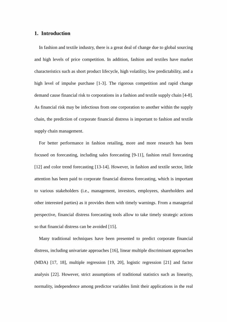
procedure to set up a BPNN includes: (1) Select input and output variables; (2)

Determine layers and number of neurons in hidden layers; (3) Learn or train from real

data; (4) Test; (5) Recall. Let q be the number of hidden nodes and p be the

dimension of the input vector (the lagged observations). The relationship between the

output (t

y ) and the inputs (T

x ) has the following mathematical representation:

t

q

j

p

i

Tiijjjtxgy

1 1

00)( (9)

where j

( j =0, 1, 2, …, q ) is the connection weight of the j th hidden node, ij

( i =0, 1, 2, …, p ) is the connection weight between the i th input node and the j th

hidden node. The logistic function is often used as the hidden layer transfer function

as follows:

)exp(1

1)(

xxg

. (10)

The BPNN model performs a nonlinear functional mapping from inputs (T

x ) to t

y

as follows.

tTtxfy ),( (11)

where is a vector of all parameters and f is a function determined by the

network structure and connection weights. Thus, the neural network is equivalent to a

nonlinear autoregressive model.

However, individual methods for corporate financial distress forecasting have

disadvantage for error recognition. Therefore, in the following section, a novel

ensemble learning approach based on logistic regression and SVM / BPNN is

proposed for error recognition and the improvement of forecasting performance.

3. A novel ensemble learning approach

Many hybrid methods have been used for economic forecasting [39-41], and risk

analysis has addressed in supply chain management [42-48]. When the methods of LR,

SVM and BPNN are used for corporate financial distress forecasting, financial ratio

indices of companies are input variables and corresponding corporate financial state

(0/1) of companies is the output. The principle of the new ensemble learning approach

based on LR and SVM/BPNN is that the forecasting results of corporate financial

distress by LR are set as another input variable within the SVM/BPNN framework,

corresponding to the output of corporate financial state. In this way, both Type I error

(reject-true error) and Type II error (accept-false error) in LR analysis can be

recognized by SVM/BPNN.

In summary, the overall process of the ensemble learning approach (LR-

SVM/BPNN) can be described in Fig. 1 as following three main steps:

(1) Stepwise regression analysis is used to remove independent variables which are

insignificantly linear with the dependent variable. In this way, remained

independent variables are significant to the dependent variable and

multicollinearity is removed.

(2) Logistic regression analysis is implemented based on train sample set. Then,

critical value of financial distress probability is set as 0.5. If the probability is

more than 0.5, the value is 1 and the company is predicted to be financial distress;

or else, the value is 0 and the company is predicted to be no financial distress.

(3) The forecasting results by LR are introduced into the SVM/BPNN technique as a

new variable. Then, there will be a new forecasting result by the LR- SVM/BPNN

approach.

Data preprocessing

Results

Financial data

Stepwise regression analysis

Valid variables

SVM / BPNN

Logistic regression

Forecasting results

Fig. 1 Framework of the proposed ensemble learning approach

On the whole, Logistic regression is a linear model, while SVM/BPNN is nonlinear

model. When the forecasting results by LR are introduced into the SVM/BPNN

technique as an input variable, SVM/BPNN can recognize the forecasting errors in

fitness by LR. Therefore, the ensemble learning approach LR-SVM/BPNN is

promising to achieve better forecasting performance.

4. Empirical analysis

4.1 Data description and experiment design

Fashion and textile sector is a traditional main industry in China. In recent years,

China’s export in fashion and textile sector is more than 25% in the global trade.

However, many fashion and textile companies have been shocked immensely since

the financial crisis in 2008. When a fashion and textile company suffers from

financial distress, other companies in its supply chains will be subjected to financial

risk. Therefore, financial distress forecasting is important in fashion and textiles

supply chains.

In this study, the data for our experiment were collected from the Shanghai Stock

Exchange and Shenzhen Stock Exchange databases in China. In 2012, there are 88

fashion and textiles related listed companies such as Shenzhen Victor Onward Textile

Industrial Co., Ltd. (000018), Xinlong Holding (Group) Company Ltd. (000955),

Hubei Maiya Co., Ltd. (000971), Shandong Demian Incorporated Company (002072),

Lanzhou Sanmao Industrial Co., Ltd. (000779), Ningxia Zhongyin Cashmere Co. Ltd.

(000982), Sichuan Langsha Holding Ltd. (600137), Hunan Huasheng Co., Ltd.

(600156), Xinjiang Tianshan Wool Tex Stock Co., Ltd. (000813), Nanjing Textiles

Import & Export Corp., Ltd. (600250), Henan Xinye Textile Co., Ltd. (002087) and

so on, where numbers in brackets are stock codes of corresponding listed companies.

We selected 15 companies once special-treated (ST) and 45 non-ST companies as

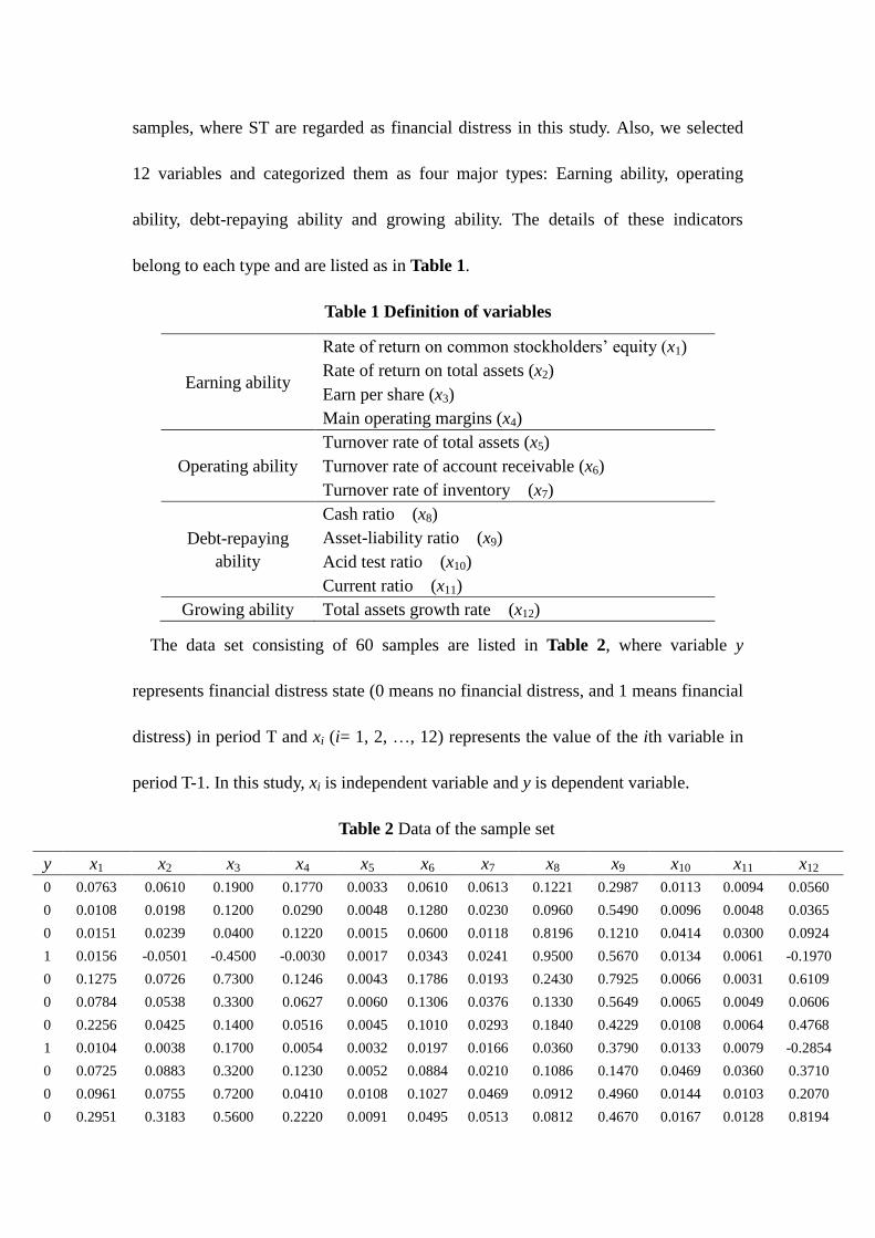
samples, where ST are regarded as financial distress in this study. Also, we selected

12 variables and categorized them as four major types: Earning ability, operating

ability, debt-repaying ability and growing ability. The details of these indicators

belong to each type and are listed as in Table 1.

Table 1 Definition of variables

Earning ability

Rate of return on common stockholders’ equity (x1)

Rate of return on total assets (x2)

Earn per share (x3)

Main operating margins (x4)

Operating ability

Turnover rate of total assets (x5)

Turnover rate of account receivable (x6)

Turnover rate of inventory (x7)

Debt-repaying

ability

Cash ratio (x8)

Asset-liability ratio (x9)

Acid test ratio (x10)

Current ratio (x11)

Growing ability Total assets growth rate (x12)

The data set consisting of 60 samples are listed in Table 2, where variable y

represents financial distress state (0 means no financial distress, and 1 means financial

distress) in period T and xi (i= 1, 2, …, 12) represents the value of the ith variable in

period T-1. In this study, xi is independent variable and y is dependent variable.

Table 2 Data of the sample set

y x1 x2 x3 x4 x5 x6 x7 x8 x9 x10 x11 x12

0 0.0763 0.0610 0.1900 0.1770 0.0033 0.0610 0.0613 0.1221 0.2987 0.0113 0.0094 0.0560

0 0.0108 0.0198 0.1200 0.0290 0.0048 0.1280 0.0230 0.0960 0.5490 0.0096 0.0048 0.0365

0 0.0151 0.0239 0.0400 0.1220 0.0015 0.0600 0.0118 0.8196 0.1210 0.0414 0.0300 0.0924

1 0.0156 -0.0501 -0.4500 -0.0030 0.0017 0.0343 0.0241 0.9500 0.5670 0.0134 0.0061 -0.1970

0 0.1275 0.0726 0.7300 0.1246 0.0043 0.1786 0.0193 0.2430 0.7925 0.0066 0.0031 0.6109

0 0.0784 0.0538 0.3300 0.0627 0.0060 0.1306 0.0376 0.1330 0.5649 0.0065 0.0049 0.0606

0 0.2256 0.0425 0.1400 0.0516 0.0045 0.1010 0.0293 0.1840 0.4229 0.0108 0.0064 0.4768

1 0.0104 0.0038 0.1700 0.0054 0.0032 0.0197 0.0166 0.0360 0.3790 0.0133 0.0079 -0.2854

0 0.0725 0.0883 0.3200 0.1230 0.0052 0.0884 0.0210 0.1086 0.1470 0.0469 0.0360 0.3710

0 0.0961 0.0755 0.7200 0.0410 0.0108 0.1027 0.0469 0.0912 0.4960 0.0144 0.0103 0.2070

0 0.2951 0.3183 0.5600 0.2220 0.0091 0.0495 0.0513 0.0812 0.4670 0.0167 0.0128 0.8194

1 -0.2065 -0.0239 -0.6700 -0.1801 0.0025 0.0297 0.0153 0.0214 0.7680 0.0057 0.0033 0.0289

0 0.0267 0.0291 0.0700 0.0248 0.0052 0.1846 0.0269 -0.1190 0.5268 0.0124 0.0076 0.0277

0 0.0511 0.0446 0.1800 0.0347 0.0107 0.0905 0.0901 0.0702 0.2570 0.0270 0.0236 0.3270

0 0.0456 0.0384 0.2500 0.0660 0.0033 0.0969 0.0076 -0.0270 0.4795 0.0167 0.0078 0.1797

1 -0.6343 -0.8480 -0.7800 -0.1544 0.0002 0.0048 0.0095 -0.0858 0.6199 0.0017 0.0014 -0.2280

0 0.1319 0.1132 0.5000 0.0880 0.0061 0.0461 0.0257 0.0965 0.5983 0.0105 0.0070 0.3730

0 0.1264 0.1365 0.2800 0.0701 0.0115 0.1525 0.0572 0.0680 0.6140 0.0080 0.0053 0.1741

0 0.0860 0.0554 0.6400 0.1130 0.0050 0.0503 0.0128 0.1040 0.4122 0.0166 0.0105 0.6068

1 -0.1326 -0.0199 -0.5700 -0.3669 0.0012 0.0085 0.0126 0.1151 0.9496 0.0059 0.0044 -0.0895

0 0.0429 0.0374 0.2000 0.0570 0.0030 0.0393 0.0275 0.1067 0.6500 0.0093 0.0071 0.1070

0 0.0259 0.0380 0.1600 0.0267 0.0047 0.0757 0.0231 0.0600 0.5230 0.0097 0.0057 0.1204

0 0.1319 0.0891 0.5000 0.0880 0.0061 0.0461 0.0257 0.0960 0.6000 0.0105 0.0070 0.8305

1 0.2490 -0.0314 -0.4300 -0.9043 0.0022 0.0200 0.0066 1.1200 0.8100 0.0103 0.0062 -0.0087

0 0.1531 0.2057 0.5900 0.1046 0.0148 0.1115 0.0225 0.0745 0.3946 0.0223 0.0148 0.8600

0 0.0458 0.0449 0.3100 0.0980 0.0024 0.0160 0.0139 0.1020 0.5500 0.0449 0.0458 0.2020

0 0.0373 0.0414 1.6200 0.0834 0.0037 0.0233 0.0246 0.1980 0.1030 0.0865 0.0735 -0.0475

1 -0.0697 -0.0270 -0.5700 0.1307 0.0024 0.0176 0.0081 0.0468 0.4403 0.0141 0.0084 0.2190

0 0.2975 0.2130 0.6100 0.0803 0.0240 0.6377 0.0590 0.0711 0.6400 0.0092 0.0057 0.7032

0 0.0462 0.0427 0.2700 0.0754 0.3400 0.0345 0.0223 0.0640 0.4870 0.0106 0.0080 0.1002

0 0.0562 0.0605 0.4500 0.0369 0.0034 0.0547 0.0242 0.0295 0.3440 0.0210 0.0177 -0.0348

1 -0.3361 -0.1000 -0.4900 0.5420 0.0020 0.0170 0.0047 0.0845 0.5760 0.0123 0.0057 0.2414

0 0.0368 0.0373 0.2200 0.0890 0.0040 0.0543 0.0265 0.1300 0.4790 0.0086 0.0055 0.0306

0 0.0647 0.0759 0.2300 0.1170 0.0050 0.2683 0.0202 0.2110 0.1849 0.0396 0.0278 0.5052

0 -0.0844 -0.0413 1.0700 -0.0501 0.0109 0.1038 0.0618 0.0100 0.6498 0.0093 0.0070 0.1459

1 -0.0740 -0.0329 -0.5100 0.1145 0.0031 0.0222 0.0254 -0.1030 0.3406 0.0160 0.0122 0.1555

0 0.0353 0.0276 0.3600 0.0172 0.0116 0.1321 0.1134 0.0035 0.4608 0.0168 0.0140 0.0155

0 0.0100 0.0129 0.0300 0.0040 0.0052 0.0469 0.0148 0.0640 0.6397 0.0100 0.0051 -0.1158

0 0.0697 0.0972 0.8800 0.1283 0.0046 0.0914 0.0168 0.0488 0.2510 0.0558 0.0465 0.6702

1 -0.0164 -0.9775 0.0300 -0.0373 0.0030 0.0287 0.0299 0.0676 0.0928 0.0651 0.0810 0.0183

0 0.0675 0.0711 0.3600 0.0890 0.0060 0.0643 0.0331 0.0690 0.0025 0.0353 0.0272 0.6003

0 0.1286 0.0988 0.7400 0.1502 0.0049 0.1340 0.0361 0.0870 0.0314 0.0601 0.0233 -0.7820

0 0.0095 0.0089 0.2100 0.0047 0.0049 0.0769 1.3050 0.1180 0.7420 0.9100 0.4370 -0.1620

1 -0.5781 -0.0467 -0.5700 -0.1924 0.0038 0.0991 0.0340 0.0012 0.5180 0.0087 0.0072 -0.0439

0 0.0517 0.0591 0.6200 0.0007 0.0063 0.0371 0.0232 -0.2009 0.2620 0.0255 0.0201 -0.0660

0 0.1323 0.0988 0.9000 0.1397 0.0049 0.0440 0.0228 0.1470 0.4730 0.0179 0.0135 0.1742

0 0.0067 0.0117 0.0200 0.0250 0.0013 0.0509 0.0138 0.0910 0.5044 0.0126 0.0113 0.0357

1 -0.1459 -0.0001 -0.7800 -0.0456 0.0046 0.0850 0.0255 -0.1059 0.6859 0.0085 0.0058 0.1287

0 0.0199 0.0223 0.1200 0.0294 0.0046 0.0774 0.0526 0.0703 0.2575 0.0160 0.0126 0.0919

0 0.0756 0.0626 0.4800 0.0787 0.0052 0.0468 0.0117 0.0200 0.4694 0.0161 0.0064 0.1685

0 0.0319 0.0448 0.1600 0.0520 0.0053 0.0586 0.0413 0.1119 0.5785 0.0631 0.0504 0.1154

1 0.1256 0.0158 0.1500 -0.0792 0.0018 0.0399 0.0159 0.1130 0.0620 0.0078 0.0005 0.0186

0 -0.2245 0.0051 -0.1400 -0.0513 0.0045 0.0491 0.0340 0.0781 0.8475 0.0045 0.0029 -0.0525

0 0.0605 0.0577 0.2700 0.0636 0.0067 0.0987 0.0448 0.0852 0.2997 0.0122 0.0076 0.2740

0 0.0939 0.1019 0.9500 0.2602 0.0037 0.1154 0.0098 0.1597 0.1496 0.0572 0.0473 0.1090

1 -0.1652 -0.1967 -2.1300 -0.0291 0.0007 0.0193 0.0009 0.4450 0.9094 0.0117 0.0094 -0.4476

0 0.0361 0.0426 0.5500 0.0339 0.0068 0.0778 0.0217 0.0335 0.4201 0.0164 0.0095 0.1240

0 0.0086 0.0163 0.0300 0.0102 0.0052 0.0747 0.0308 0.0350 0.4217 0.0123 0.0080 0.0984

0 0.0135 0.0208 0.0400 0.0147 0.0033 0.0902 0.0361 0.1088 0.4901 0.0083 0.0067 0.0711

1 0.1437 0.1113 0.3700 0.1548 0.0061 0.0269 0.0200 0.0856 0.4080 0.0197 0.0197 1.5970

The training set (first 40 samples in Table 2) and the testing set (last 20 samples in

Table 2) used in empirical analysis are described in Table 3. Here, the training set is

used to acquire the parameters of forecasting models, while the testing set is used to

measure the forecasting performance of forecasting models.

Table 3 Training set and testing set

Sample Distressed set Non-distressed set Total

Training set 10 30 40

Testing set 5 15 20

Total 15 45 60

4.2 Experiment results and analysis

In the empirical analysis of corporate financial distress forecasting, financial state

of listed companies in period T is dependent variable/output and variables in period

T-1 are input. Normalization of variables in period T-1 is implemented and the

normalized value is listed in Table 4.

Table 4 Normalized value of variables in period T-1

x1 x2 x3 x4 x5 x6 x7 x8 x9 x10 x11 x12

0.5252 0.6029 0.2373 0.4953 -0.9818 -0.8224 -0.9074 -0.5109 -0.3745 -0.9789 -0.9592 -0.2955

0.3846 0.5393 0.2000 0.2906 -0.9729 -0.6107 -0.9661 -0.5505 0.1540 -0.9826 -0.9803 -0.3119

0.3939 0.5456 0.1573 0.4192 -0.9923 -0.8256 -0.9833 0.5452 -0.7498 -0.9126 -0.8648 -0.2649

0.3949 0.4314 -0.1040 0.2464 -0.9912 -0.9068 -0.9644 0.7426 0.1921 -0.9742 -0.9743 -0.5082

0.6351 0.6208 0.5253 0.4228 -0.9759 -0.4508 -0.9718 -0.3279 0.6683 -0.9892 -0.9881 0.1710

0.5297 0.5918 0.3120 0.3372 -0.9659 -0.6025 -0.9437 -0.4944 0.1876 -0.9894 -0.9798 -0.2916

0.8457 0.5743 0.2107 0.3219 -0.9747 -0.6960 -0.9564 -0.4172 -0.1122 -0.9800 -0.9730 0.0583

0.3838 0.5146 0.2267 0.2580 -0.9823 -0.9529 -0.9759 -0.6413 -0.2049 -0.9745 -0.9661 -0.5825

0.5171 0.6450 0.3067 0.4206 -0.9706 -0.7358 -0.9692 -0.5314 -0.6949 -0.9005 -0.8373 -0.0307

0.5677 0.6253 0.5200 0.3072 -0.9376 -0.6906 -0.9295 -0.5577 0.0421 -0.9720 -0.9551 -0.1686

0.9948 1.0000 0.4347 0.5575 -0.9476 -0.8587 -0.9227 -0.5729 -0.0191 -0.9670 -0.9436 0.3463

-0.0818 0.4718 -0.2213 0.0015 -0.9865 -0.9213 -0.9779 -0.6634 0.6165 -0.9912 -0.9872 -0.3183

0.4188 0.5536 0.1733 0.2848 -0.9706 -0.4318 -0.9601 -0.8760 0.1072 -0.9764 -0.9675 -0.3193

0.4711 0.5776 0.2320 0.2985 -0.9382 -0.7292 -0.8632 -0.5895 -0.4626 -0.9443 -0.8942 -0.0677

0.4593 0.5680 0.2693 0.3418 -0.9818 -0.7090 -0.9897 -0.7367 0.0073 -0.9670 -0.9666 -0.1915

-1.0000 -0.8001 -0.2800 0.0370 -1.0000 -1.0000 -0.9868 -0.8257 0.3038 -1.0000 -0.9959 -0.5343

0.6446 0.6834 0.4027 0.3722 -0.9653 -0.8695 -0.9620 -0.5497 0.2582 -0.9806 -0.9702 -0.0290

0.6328 0.7194 0.2853 0.3474 -0.9335 -0.5333 -0.9137 -0.5929 0.2913 -0.9861 -0.9780 -0.1962

0.5460 0.5942 0.4773 0.4068 -0.9717 -0.8562 -0.9817 -0.5383 -0.1348 -0.9672 -0.9542 0.1675

0.0768 0.4780 -0.1680 -0.2569 -0.9941 -0.9883 -0.9821 -0.5215 1.0000 -0.9908 -0.9821 -0.4178

0.4535 0.5664 0.2427 0.3293 -0.9835 -0.8910 -0.9592 -0.5343 0.3673 -0.9833 -0.9698 -0.2526

0.4170 0.5674 0.2213 0.2874 -0.9735 -0.7760 -0.9660 -0.6050 0.0991 -0.9824 -0.9762 -0.2414

0.6446 0.6462 0.4027 0.3722 -0.9653 -0.8695 -0.9620 -0.5505 0.2617 -0.9806 -0.9702 0.3556

0.8959 0.4603 -0.0933 -1.0000 -0.9882 -0.9520 -0.9913 1.0000 0.7052 -0.9811 -0.9739 -0.3499

0.6901 0.8262 0.4507 0.3951 -0.9141 -0.6628 -0.9669 -0.5830 -0.1720 -0.9546 -0.9345 0.3804

0.4598 0.5780 0.3013 0.3860 -0.9871 -0.9646 -0.9801 -0.5414 0.1562 -0.9049 -0.7924 -0.1728

0.4415 0.5726 1.0000 0.3658 -0.9794 -0.9415 -0.9637 -0.3960 -0.7878 -0.8133 -0.6655 -0.3825

0.2118 0.4670 -0.1680 0.4312 -0.9871 -0.9596 -0.9890 -0.6250 -0.0755 -0.9727 -0.9638 -0.1585

1.0000 0.8375 0.4613 0.3615 -0.8599 1.0000 -0.9109 -0.5882 0.3462 -0.9835 -0.9762 0.2486

0.4606 0.5746 0.2800 0.3548 1.0000 -0.9061 -0.9672 -0.5989 0.0231 -0.9804 -0.9656 -0.2583

0.4821 0.6021 0.3760 0.3015 -0.9812 -0.8423 -0.9643 -0.6511 -0.2789 -0.9575 -0.9212 -0.3718

-0.3599 0.3544 -0.1253 1.0000 -0.9894 -0.9614 -0.9942 -0.5679 0.2111 -0.9767 -0.9762 -0.1396

0.4404 0.5663 0.2533 0.3736 -0.9776 -0.8436 -0.9607 -0.4990 0.0062 -0.9848 -0.9771 -0.3169

0.5003 0.6259 0.2587 0.4123 -0.9717 -0.1673 -0.9704 -0.3763 -0.6148 -0.9165 -0.8749 0.0821

0.1803 0.4450 0.7067 0.1812 -0.9370 -0.6872 -0.9066 -0.6807 0.3669 -0.9833 -0.9702 -0.2199

0.2026 0.4579 -0.1360 0.4088 -0.9829 -0.9450 -0.9624 -0.8518 -0.2860 -0.9685 -0.9464 -0.2119

0.4372 0.5513 0.3280 0.2743 -0.9329 -0.5977 -0.8275 -0.6905 -0.0322 -0.9668 -0.9381 -0.3296

0.3829 0.5286 0.1520 0.2560 -0.9706 -0.8670 -0.9787 -0.5989 0.3456 -0.9817 -0.9789 -0.4399

0.5111 0.6587 0.6053 0.4279 -0.9741 -0.7263 -0.9756 -0.6219 -0.4752 -0.8809 -0.7892 0.2208

0.3263 -1.0000 0.1520 0.1989 -0.9835 -0.9245 -0.9555 -0.5935 -0.8093 -0.8604 -0.6312 -0.3272

0.5063 0.6185 0.3280 0.3736 -0.9659 -0.8120 -0.9506 -0.5913 -1.0000 -0.9260 -0.8777 0.1621

0.6375 0.6612 0.5307 0.4582 -0.9723 -0.5917 -0.9460 -0.5641 -0.9390 -0.8714 -0.8955 -1.0000

0.3818 0.5225 0.2480 0.2570 -0.9723 -0.7722 1.0000 -0.5171 0.5616 1.0000 1.0000 -0.4788

-0.8794 0.4366 -0.1680 -0.0156 -0.9788 -0.7020 -0.9492 -0.6940 0.0886 -0.9846 -0.9693 -0.3795

0.4724 0.5999 0.4667 0.2515 -0.9641 -0.8979 -0.9658 -1.0000 -0.4520 -0.9476 -0.9102 -0.3981

0.6454 0.6612 0.6160 0.4437 -0.9723 -0.8761 -0.9664 -0.4732 -0.0064 -0.9643 -0.9404 -0.1961

0.3758 0.5268 0.1467 0.2851 -0.9935 -0.8543 -0.9802 -0.5580 0.0599 -0.9760 -0.9505 -0.3126

0.0483 0.5086 -0.2800 0.1874 -0.9741 -0.7466 -0.9623 -0.8562 0.4431 -0.9850 -0.9757 -0.2344

0.4042 0.5431 0.2000 0.2912 -0.9741 -0.7706 -0.9207 -0.5894 -0.4615 -0.9685 -0.9446 -0.2653

0.5237 0.6053 0.3920 0.3593 -0.9706 -0.8673 -0.9834 -0.6655 -0.0140 -0.9683 -0.9730 -0.2009

0.4299 0.5779 0.2213 0.3224 -0.9700 -0.8300 -0.9380 -0.5264 0.2163 -0.8648 -0.7714 -0.2456

0.6310 0.5331 0.2160 0.1410 -0.9906 -0.8891 -0.9770 -0.5247 -0.8744 -0.9866 -1.0000 -0.3269

-0.1204 0.5166 0.0613 0.1796 -0.9747 -0.8600 -0.9492 -0.5776 0.7844 -0.9938 -0.9890 -0.3867

0.4913 0.5978 0.2800 0.3384 -0.9617 -0.7033 -0.9327 -0.5668 -0.3724 -0.9769 -0.9675 -0.1122

0.5630 0.6660 0.6427 0.6103 -0.9794 -0.6505 -0.9864 -0.4540 -0.6894 -0.8778 -0.7856 -0.2509

0.0069 0.2051 -1.0000 0.2103 -0.9971 -0.9542 -1.0000 -0.0220 0.9151 -0.9780 -0.9592 -0.7189

0.4389 0.5745 0.4293 0.2974 -0.9612 -0.7693 -0.9681 -0.6451 -0.1182 -0.9676 -0.9588 -0.2383

0.3799 0.5339 0.1520 0.2646 -0.9706 -0.7791 -0.9541 -0.6428 -0.1148 -0.9767 -0.9656 -0.2599

0.3904 0.5408 0.1573 0.2708 -0.9818 -0.7301 -0.9460 -0.5311 0.0297 -0.9855 -0.9716 -0.2828

0.6699 0.6805 0.3333 0.4646 -0.9653 -0.9302 -0.9707 -0.5662 -0.1437 -0.9604 -0.9120 1.0000

As a result, the methods are used for corporate financial distress forecasting in the

next period when the value of variables in current period are available. By using the

training set and the testing set in Table 3, we obtain the forecasting performance

comparison of methods with values of variables in period T-1 and financial state in

period T as in Table 5.

Table 5 Comparison of forecasting performance with variables in period T

LR BPNN SVM LR-BPNN LR-SVM

Type I error rate 46.7% 20% 13.3% 13.3% 6.7%

Type II error rate 40% 20% 40% 20% 40%

Total accuracy 55% 80% 80% 85% 85%

Moreover, independent variable values in periods T-2 and T-3 are used for

corporate financial distress (independent variable in period T) forecasting, and

comparison of forecasting performance with period T-2 and period T-3 data is shown

in Tables 6 and 7.

Table 6 Comparison of forecasting performance with variables in period T-2

LR BPNN SVM LR-BPNN LR-SVM

Type I error rate 46.7% 33.3% 26.7% 26.7% 13.3%

Type II error rate 60% 40% 40% 20% 40%

Total accuracy 50% 65% 70% 75% 80%

Table 7 Comparison of forecasting performance with variables in period T-3

LR BPNN SVM LR-BPNN LR-SVM

Type I error rate 53.3% 33.3% 26.7% 20% 26.7%

Type II error rate 60% 60% 40% 40% 20%

Total accuracy 45% 60% 70% 75% 75%

From the results in Table 5, the accuracy by BPNN and SVM is 80%, and that by

LR-BPNN and LR-SVM is 85%, which is much higher than the accuracy 50% by LR.

In addition, by comparing the results in Tables 5-7, we can find that the total accuracy

decreases in the length from current period to period T, i.e. total accuracy in period

T-1 is better than that in period T-2, which is better than that in period T-3. Therefore,

we can conclude that artificial intelligence techniques, i.e. SVM and BPNN can

achieve better forecasting performance than LR. In addition, as SVM/BPNN can

recognize the forecasting errors in fitness by LR, ensemble learning approaches

LR-BPNN and LR-SVM can achieve better forecasting performance than individual

methods when the forecasting results by LR are introduced into the SVM/BPNN

technique as an input variable.

5. Conclusions and future work

In this study, logistic regression (LR) model is integrated with artificial intelligence

tools, i.e. support vector machine (SVM) and back-propagation neural networks

(BPNN), for corporate financial distress forecasting in fashion and textiles supply

chains. Empirical analysis of Chinese listed companies in fashion and textile sector is

implemented for the comparison of the methods, and some related issues are

discussed.

The contribution of this study is that a novel ensemble learning approach is

developed for corporate financial distress forecasting in fashion and textiles supply

chains. In the framework of the proposed ensemble learning approach, the forecasting

results by LR are introduced into the SVM and BPNN techniques which can

recognize the forecasting errors in fitness by LR. The results suggest that artificial

intelligence tools are better than LR and the proposed novel ensemble learning

approach can achieve better forecasting performance than that of individual models.

By using the proposed approach, managers in fashion and textiles companies can

predict the financial state of their suppliers, manufacturers and retailers in advance

and give a quick response for better supply chain performance.

It is expected that future research would benefit from concentrating on other

methods for corporate financial distress forecasting, using data from a wider sample

of fashion and textiles companies.

Acknowledgements

We sincerely thank the anonymous referees for their valuable suggestions and

comments. This work was supported by the National Natural Science Foundation of

China (No. 70871107, 71101028), China Postdoctoral Science Foundation (Grant No.

20060400103), the Program for Innovative Research Team in UIBE and The Royal

Academy of Engineering for research exchanges with China and India scheme.

References

[1] M. Christopher, R. Lowson and H. Peck, “Creating agile supply chains in the

fashion industry,” International Journal of Retail & Distribution Management,

vol. 32, no. 8, pp. 367-376, 2004.

[2] M. Bruce, L. Daly and N. Towers, “Lean or agile: A solution for supply chain

management in the textiles and clothing industry?” International Journal of

Operations & Production Management, vol. 24, no. 2, pp.151-170, 2004.

[3] M.P. de Brito, V. Carbone and C.M. Blanquart, “Towards a sustainable fashion

retail supply chain in Europe: Organisation and performance,” International

Journal of Production Economics, vol. 114, no. 2, pp. 534-553, 2008.

[4] P. Hilletofth and O.-P. Hilmola, “Supply chain management in fashion and textile

industry,” International Journal of Services Sciences, vol. 1, no. 2, pp. 127-147,

2008.

[5] S. Thomassey, “Sales forecasts in clothing industry: The key success factor of the

supply chain management,” International Journal of Production Economics, vol.

128, no. 2, pp. 470-483, 2010.

[6] L. Barnes and G. Lea-Greenwood, “Fast fashioning the supply chain: shaping the

research agenda,” Journal of Fashion Marketing and Management, vol. 10, no. 3

pp. 259-271, 2006.

[7] G. Birtwistle, N. Siddiqui and S.S. Fiorito, “Quick response: perceptions of UK

fashion retailers,” International Journal of Retail & Distribution Management,

vol. 31, no. 2, pp. 118-128, 2003.

[8] S.G. Hayes and N. Jones, “Fast fashion: a financial snapshot,” Journal of Fashion

Marketing and Management, vol. 10, no. 3, pp. 282 - 300, 2006.

[9] Z.L. Sun, T.M. Choi, K.F. Au and Y. Yu. “Sales forecasting using extreme

learning machine with applications in fashion retailing,” Decision Support

Systems, vol. 46, pp. 411-419, 2008.

[10] T.M. Choi, Y. Yu and K.F. Au, “A hybrid SARIMA wavelet transform method for

sales forecasting,” Decision Support Systems, vol. 51, no. 1, pp. 130-140, 2011.

[11] Y. Yu, T.M. Choi and C.L. Hui, “An intelligent fast sales forecasting model for

fashion products,” Expert Systems with Applications, vol. 38, pp. 7373-7379,

2011.

[12] K.F. Au, T.M. Choi and Y. Yu, “Fashion retail forecasting by using evolutionary

neural networks,” International Journal of Production Economics, vol. 114, pp.

615-630, 2008.

[13] Y. Yu, C.L. Hui and T.M. Choi, “An empirical study of intelligent expert systems

on forecasting of fashion color trend,” Expert Systems with Applications, vol. 39,

pp. 4383-4389, 2012.

[14] T.M. Choi, C.L. Hui, SF.F. Ng and Y. Yu, “Color trend forecasting of fashionable

products with very few historical data,” IEEE Transactions on Systems, Man, and

Cybernetics, Part C, vol. 42, pp. 1003-1010, 2012.

[15] Z. Hua, Y. Wang, X. Xu, B. Zhang and L. Liang, “Predicting corporate financial

distress based on integration of support vector machine and logistic regression,”

Expert Systems with Applications, vol. 33, no. 2, pp. 434-440, 2007.

[16] W. Beaver, “Financial ratios as predictors of failure, empirical research in

accounting: Selected studied,” Journal of Accounting Research, vol. 4, pp. 71-111,

1968.

[17] E.L. Altman, “Financial ratios, discriminant analysis and the prediction of

corporate bankruptcy,” The Journal of Finance, vol. 23, no. 3, pp. 589-609, 1968.

[18] M. Blum, “Failing company discriminant analysis,” Journal of Accounting

Research, vol. 12, no. 1, pp. 1-25, 1974.

[19] E.L. Altman, I. Edward, R. Haldeman and P. Narayanan, “A new model to

identify bankruptcy risk of corporations,” Journal of Banking and Finance, vol. 1,

pp. 29-54, 1977.

[20] P.A. Meyer and H. Pifer, “Prediction of bank failures,” The Journal of Finance,

vol. 25, pp. 853-868, 1970.

[21] E.K. Laitinen and T. Laitinen, “Bankruptcy prediction application of the Taylor’s

expansion in logistic regression,” International Review of Financial Analysis, vol.

9, pp. 327-349, 2000.

[22] A.I. Dimitras, S.H. Zanakis and C. Zopounidis, “A survey of business failure with

an emphasis on prediction methods and industrial applications,” European

Journal of Operational Research, vol. 90, no. 3, pp. 487-513, 1996.

[23] M.-Y. Chen, “Predicting corporate financial distress based on integration of

decision tree classification and logistic regression,” Expert Systems with

Applications, vol. 38, no. 9, pp. 11261-11272, 2011.

[24] W.-S. Chen and Y.-K. Du, “Using neural networks and data mining techniques for

the financial distress prediction model,” Expert Systems with Applications, vol. 36,

no. 2, pp. 4075-4086, 2009.

[25] H. Li and J. Sun, “Ranking-order case-based reasoning for financial distress

prediction,” Knowledge-Based Systems, vol. 21, pp. 868-878, 2008.

[26] H. Li and J. Sun, “Gaussian case-based reasoning for business failure prediction

with empirical data in China,” Information Sciences, vol. 179, pp. 89-108, 2009.

[27] K. Kim and H. Ahn, “A corporate credit rating model using multi-class support

vector machines with an ordinal pairwise partitioning approach,” Computers &

Operations Research, vol. 39, no. 8, pp. 1800-1811, 2012.

[28] J. Sun and H. Li, “Financial distress prediction using support vector machines:

Ensemble vs. individual,” Applied Soft Computing, vol. 12, pp. 2254-2265, 2012.

[29] C.-J. Lu, T.-S. Lee and C.-C. Chiu, “Financial time series forecasting using

independent component analysis and support vector regression,” Decision

Support Systems, vol. 47, pp. 115-125, 2009.

[30] Z. Xiao, X. Yang, Y. Pang and X. Dang, “The prediction for listed companies’

financial distress by using multiple prediction methods with rough set and

Dempster-Shafer evidence theory,” Knowledge-Based Systems, vol. 26, pp.

196-206, 2012.

[31] J. Sun, M. Jia and H. Li, “AdaBoost ensemble for financial distress prediction:

An empirical comparison with data from Chinese listed companies,” Expert

Systems with Applications, vol. 38, pp. 9305-9312, 2011.

[32] H. Li and J. Sun, “Empirical research of hybridizing principal component

analysis with multivariate discriminant analysis and logistic regression for

business failure prediction,” Expert Systems with Applications, vol. 38, pp.

6244-6253, 2011.

[33] D.W. Hosmer and S. Lemeshow, Applied logistic regression, Wiley, New York,

2000.

[34] V. Vapnik, The nature of statistical learning theory, Springer-Verlag, NewYork,

1995.

[35] P.G. Harrald and M. Kamstra, “Evolving artificial neural networks to combine

financial forecasts,” IEEE Transactions on Evolutionary Computation, vol. 1, no.

1, pp. 40-52, 1997.

[36] C. Hamzacebia, D. Akayb and F. Kutayb, “Comparison of direct and iterative

artificial neural network forecast approaches in multi-periodic time series

forecasting,” Expert Systems with Applications, vol. 36, no. 2, pp. 3839-3844,

2009.

[37] J.V. Hansen and R.D. Nelson, “Neural networks and traditional time series

methods: A synergistic combination in state economic forecasts,” IEEE

Transactions on Neural Networks, vol. 8, no. 4, pp. 863-873, 1997.

[38] W. Leigh, R. Purvis and J.M. Ragusa, “Forecasting the NYSE composite index

with technical analysis, pattern recognizer, neural network, and genetic algorithm:

A case study in romantic decision support,” Decision Support Systems, vol. 32, no.

4, pp. 361-377, 2002.

[39] B. Majhi, M. Rout, R. Majhi, G. Panda and P.J. Fleming, “New robust forecasting

models for exchange rates prediction,” Expert Systems with Applications, vol. 39,

no. 16, pp. 12658-12670, 2012.

[40] Z.L. Sun, K.F. Au and T.M. Choi, “A neuro-fuzzy inference system through

integration of fuzzy logic and extreme learning machines,” IEEE Transactions on

Systems, Man, and Cybernetics – Part B: Cybernetics, vol. 37, no. 5, pp.

1321-1331, 2007.

[41] B. Premanode and C. Toumazou, “Improving prediction of exchange rates using

Differential EMD.” Expert Systems with Applications, vol. 40, no. 1, pp. 377-384,

2013.

[42] G. Xie, W. Yue, W. Liu and S. Wang, “Risk based selection of cleaner products in

a green supply chain,” Pacific Journal of Optimization, vol. 8, no. 3, pp. 473-484,

2012.

[43] G. Xie, S. Wang and K.K. Lai, “Quality improvement in competing supply

chains,” International Journal of Production Economics, vol. 134, no. 1, pp.

262-270, 2011.

[44] G. Xie, W. Yue, S. Wang and K.K. Lai, “Quality investment and price decision in

a risk-averse supply chain,” European Journal of Operational Research, vol. 214,

no. 2, pp. 403-410, 2011.

[45] G. Xie, S. Wang and K.K. Lai, “Optimal βk-stable interval in VPRS-based group

decision-making: A further application,” Expert Systems with Applications, vol.

38, no. 11, pp. 13757-13763, 2011.

[46] G. Xie, W. Yue, S. Wang and K.K. Lai, “Dynamic risk management in petroleum

project investment based on a variable precision rough set model,” Technological

Forecasting & Social Change, vol. 77, no. 6, pp. 891-901, 2010.

[47] G. Xie, W. Yue and S. Wang, “VPRS-based group decision-making for risk

response in petroleum investment,” International Journal of Knowledge and

Systems Sciences, vol. 1, no. 3, pp. 45-54, 2010.

[48] G. Xie, J. Zhang, K.K. Lai and L. Yu, “Variable precision rough set for group

decision-making: An application,” International Journal of Approximate

Reasoning, vol. 49, no. 2, pp. 331-343, 2008.