a novel computational algorithm for predicting immune cell
TRANSCRIPT

A novel computational algorithm for
predicting immune cell types using single-cell
RNA sequencing data
By
Shuo Jia
A hesis submitted to the Faculty of Graduate Studies of
The University of Manitoba
n partial fulfillment of the requirements of the degree of
MASTER OF SCIENCE
Department of Biochemistry and Medical Genetics
University of Manitoba
Winnipeg, Manitoba, Canada
Copyright © 2020 by Shuo Jia
1
Abstract
Background: Cells from our immune system detect and kill pathogens to protect our body
against many diseases. However, current methods for determining cell types have some
major limitations, such as being time-consuming and with low throughput rate, etc. These
problems stack up and hinder the deep exploration of cellular heterogeneity. Immune cells
that are associated with cancer tissues play a critical role in revealing the stages of tumor
development. Identifying the immune composition within tumor microenvironments in a
timely manner will be helpful to improve clinical prognosis and therapeutic management
for cancer. Single-cell RNA sequencing (scRNA-seq), an RNA sequencing (RNA-seq)
technique that focuses on a single cell level, has provided us with the ability to conduct cell
type classification. Although unsupervised clustering approaches are the major methods
for analyzing scRNA-seq datasets, their results vary among studies with different input
parameters and sizes. However, in supervised machine learning methods, information loss
and low prediction accuracy are the key limitations.
Methods and Results: Genes in the human genome align to chromosomes in a particular
order. Hence, we hypothesize incorporating this information into our model will potentially
improve the cell type classification performance. In order to utilize gene positional
information, we introduce chromosome-based neural network, namely ChrNet, a novel
chromosome-specific re-trainable supervised learning method based on a one-dimensional

2
convolutional neural network (1D-CNN). The model’s performance was evaluated and
compared with other supervised learning architectures. Overall, the ChrNet showed highest
performance among the 3 models we benchmarked. In addition, we demonstrated the
advantages of our new model over unsupervised clustering approaches using gene
expression profiles from healthy, and tumor infiltrating immune cells. The codes for our
model are packed into a Python package publicly available online on Github.
Conclusions: We established an innovative chromosome-based 1D-CNN architecture to
extract scRNA-seq expression information for immune cell type classification. It is
expected that this model can become a reference architecture for future cell type
classification methods.
Keywords: convolutional neural network, immune cells, supervised learning, scRNA-seq

3
Acknowledgements
I would like to express my sincere thanks to my supervisor Dr. Pingzhao Hu. Dr. Hu
provided me with a great platform to take whatever classes I need and express my coding
knowledge freely in my project. From the very beginning of my Master’s program I could
start working on my project with my own understanding and it really came out to be a
successful project. I am grateful for all his support and guidance throughout my whole
Master’s program in the University of Manitoba.
It is also my great pleasure to have such a responsible committee. I want to thank Dr.
Kirk McManus for his professional and responsible research attitude that guided me
through each of the obstacles I faced. All of the small meet-ups with him let me realize the
downsides of my project and my scientific writing. In addition, I also want to thank Dr.
Janilyn Arsenio for her excellent expertise in immunology and very constructive
suggestions to reframe my project goals. In the end, I want to thank Dr. Meaghan Jones for
giving me insightful advices on bioinformatics part of my project. I always found it hard
for me to improve the project, and she really pointed out the essential parts of the project
to make it well-organized.
I would like to thank all my colleagues, especially Jin, for always standing by my side
on whatever troubles I had these two years. Also special thanks to Shujun, Rayhan,
Mohaiminul, Jiaying, Nikta and all other lab members from our lab.
I would like to give a shout out for my friends in North America for playing online

4
games with me to cheer me up every time when I was at my lowest.
Finally, I would like to thank my parents. Their faith in me is what finally defines me.
5
Table of contents
Abstract ...................................................................................................................................... 1
Acknowledgements ..................................................................................................................... 3
Table of contents ......................................................................................................................... 5
List of Tables .............................................................................................................................. 8
List of Equations ......................................................................................................................... 9
List of Figures ........................................................................................................................... 10
List of abbreviations .................................................................................................................. 11
Chapter 1 Background ............................................................................................................... 14
1.1. The importance of tumor-associated immune cells ..................................................... 14
1.2. Study immune heterogeneity with sequencing ............................................................ 15
1.3. Methods for cell type identification ............................................................................ 18
1.4. Major tumor-associated immune cell types ................................................................. 24
1.5. Deep learning algorithms for immune cell subtyping .................................................. 26
Chapter 2 Research Motivation, Hypothesis and Aims ............................................................... 30
2.1. Motivation ................................................................................................................. 30
2.2. Hypothesis ................................................................................................................. 31
2.3. Research aims ............................................................................................................ 31
Chapter 3 Materials and Methods .............................................................................................. 33
3.1. Data sources .............................................................................................................. 33
3.1.1. Training and validation sets ................................................................................ 34
3.1.2. Test set ............................................................................................................... 36
3.2. Preprocessing of the datasets ...................................................................................... 38
3.2.1 Introduction .............................................................................................................. 38
3.2.2 Transcripts per kilobase million (TPM) ..................................................................... 38
3.2.3 Normalization pipeline applied in our study .............................................................. 39
3.3. ChrNet: A chromosome-based 1D convolutional neural network ................................ 40
3.3.1 Rationale .................................................................................................................. 40
3.3.2 ChrNet architecture and training parameters .............................................................. 41

6
3.3.3 Introduction of major layers in ChrNet ...................................................................... 42
3.3.4 Loss function ............................................................................................................ 44
3.3.5 The gene alignment algorithm ................................................................................... 45
3.3.6 The prediction of an unlabeled single cell .................................................................. 46
3.4. Deep neural network (DNN) and support vector machine (SVM) model structures ..... 48
3.4.1 DNN structure .......................................................................................................... 48
3.4.1 SVM structure .......................................................................................................... 49
3.5. Performance evaluation .............................................................................................. 51
3.5.1 Confusion matrix ...................................................................................................... 51
3.5.2 Cross-validation ........................................................................................................ 51
3.5.3 Receiver operating characteristic (ROC) curve .......................................................... 53
3.6. Comparison with unsupervised clustering results ........................................................ 54
Chapter 4 Results and Discussion .............................................................................................. 55
4.1. Processed datasets ...................................................................................................... 55
4.2. ChrNet model construction ........................................................................................ 56
4.3. ChrNet performance evaluation .................................................................................. 59
4.3.1 Comparing ChrNet with other classification methods using 10F CV .......................... 59
4.3.2 Evaluating cell-type specific ChrNet’s performance using ROC curve ....................... 61
4.4. ChrNet potentially overcame the limitations of the unsupervised clustering approach . 63
4.4.1 Prediction of the tumor infiltrating immune cells: ChrNet vs. the Seurat unsupervised
clustering........................................................................................................................... 63
4.4.2 Prediction of the healthy immune cells: ChrNet vs. the Seurat unsupervised clustering
.......................................................................................................................................... 67
4.5. Software implementation for ChrNet .......................................................................... 71
4.5.1 Main.py .................................................................................................................... 72
4.5.2 Model.py .................................................................................................................. 73
4.5.3 Data.py ..................................................................................................................... 73
4.5.4 MetaFeature selection using IG ................................................................................. 75
Chapter 5 Significance, limitations and future direction ............................................................. 79

7
5.1. Significance ............................................................................................................... 79
5.2. Limitations ................................................................................................................ 80
5.3. Future directions ........................................................................................................ 83
References ................................................................................................................................ 84
Appendix .................................................................................................................................. 92

8
List of Tables
Table 1. The advantages and drawbacks of currently available methods ..................................... 23
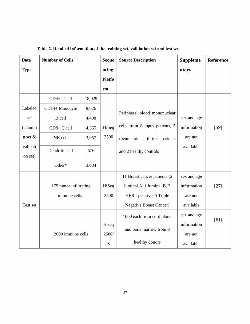
Table 2. Detailed information of the training set, validation set and test set. ............................... 37
Table 3. The list of hyperparameters used to tune the ChrNet..................................................... 42
Table 4. Pseudo code for gene alignment algorithm ................................................................... 46
Table 5. Comparing different methods’ model performance with ChrNet using 10-fold cross
validation. ................................................................................................................................. 60
Table 6. Algorithm for finding significant MetaFeatures ............................................................ 77

9
List of Equations
Equation 1 ................................................................................................................................. 39
Equation 2 ................................................................................................................................. 44
Equation 3 ................................................................................................................................. 44
Equation 4 ................................................................................................................................. 45
Equation 5 ................................................................................................................................. 51
Equation 6 ................................................................................................................................. 51
Equation 7 ................................................................................................................................. 53
Equation 8 ................................................................................................................................. 53
Equation 9 ................................................................................................................................. 53
Equation 10 ............................................................................................................................... 75

10
List of Figures
Figure 1. Supervised learning vs. unsupervised learning ............................................................ 19
Figure 2. Illustration of different cell type identification methods. ............................................. 21
Figure 3. The hierarchical structure of CNN .............................................................................. 27
Figure 4. The overall workflow of this project. .......................................................................... 32
Figure 5. The splitting algorithm applied for generating training set and validation set. .............. 35
Figure 6. The layout of ChrNet architecture. .............................................................................. 42
Figure 7. The pipeline for prediction.......................................................................................... 47
Figure 8. The DNN model applied in our study.......................................................................... 49
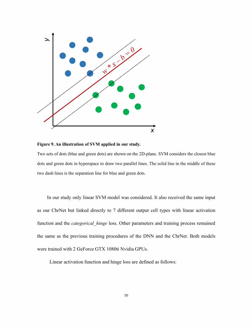
Figure 9. An illustration of SVM applied in our study. ............................................................... 50
Figure 10. An illustration of 10F CV. ........................................................................................ 52
Figure 11. Distributions of the number of cells in each of the cell types in the training set and
validation set applied to constructing the ChrNet. ...................................................................... 56
Figure 12. The confusion matrix of the prediction results for each cell type in the validation set. 58
Figure 13. The fold-specific accuracy of the three models in the 10-fold cross validation
procedure. ................................................................................................................................. 59
Figure 14. ChrNet-based multiclass ROCs. ................................................................................ 62
Figure 15. Comparisons of the Seurat unsupervised clustering predictions with our ChrNet’s
predictions of the 175 tumor infiltrating immune cells. .............................................................. 64
Figure 16. The distributions of the expression levels of the four selected marker genes in the 175
tumor infiltrating immune cells by the unsupervised clustering. ................................................. 66
Figure 17. Comparison of the Seurat unsupervised clustering predictions with ChrNet’s
predictions using the 2000 immune cells from the 8 healthy donors. .......................................... 67
Figure 18. The distributions of the expression levels of the four selected marker genes in the 2000
immune cells from the 8 healthy donors by the unsupervised clusters. ....................................... 70
Figure 19. Homepage of ChrNet online repository. .................................................................... 72
11
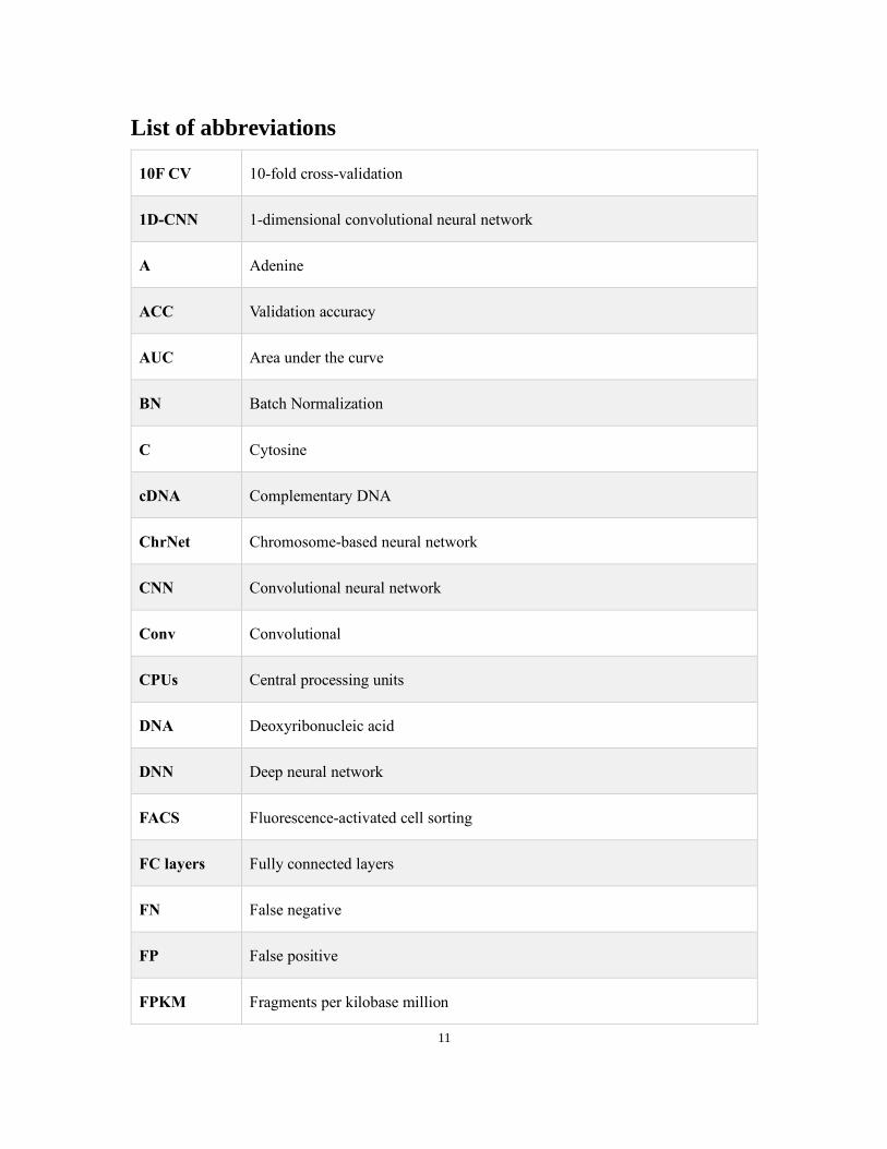
List of abbreviations
10F CV 10-fold cross-validation
1D-CNN 1-dimensional convolutional neural network
A Adenine
ACC Validation accuracy
AUC Area under the curve
BN Batch Normalization
C Cytosine
cDNA Complementary DNA
ChrNet Chromosome-based neural network
CNN Convolutional neural network
Conv Convolutional
CPUs Central processing units
DNA Deoxyribonucleic acid
DNN Deep neural network
FACS Fluorescence-activated cell sorting
FC layers Fully connected layers
FN False negative
FP False positive
FPKM Fragments per kilobase million

12
G Guanine
GPUs Graphics processing units
HCA Human Cell Atlas
HER2 Human epidermal growth factor receptor 2
MaxP Max Pooling
mRNA Messenger RNA
NGS Next generation sequencing
NK cell Natural killer cell
PBMC Peripheral blood mononuclear cell
ReLU Rectified linear unit
RNA-seq RNA sequencing
RNA Ribonucleic acid
ROC Receiver operating characteristic
RPKM Reads per kilobase million
scRNA-seq Single-cell RNA sequencing
SNP Single nucleotide polymorphism
SVM Support vector machine
T Thymine
t-SNE T-Distributed Stochastic Neighbor Embedding
TIL Tumor infiltrating lymphocyte
13
TN True negative
TNBC Triple negative breast cancer
TP True positive
TPM Transcripts per kilobase million

14
Chapter 1 Background
1.1. The importance of tumor-associated immune cells
Understanding cellular heterogeneity is crucial in determining human health status.
Different cell populations in the human body function together to keep the body healthy.
Pathological research showed that heterogeneity was found in the majority of human
tumors [1]. By studying heterogeneity in different health states, researchers may unravel
the key to treat many complex diseases, for example, cancers.
However, not all cellular differences are equally important to be explored, and
accurate modeling of cell populations should focus on those cell types that are most
relevant to health [2]. White blood cells from our immune system detect and kill pathogens
to protect our body against many diseases. These cells produce cytokines and antibodies,
as well as killing extra cellular substances in response to all disease statuses [3].
Monitoring the human immune system is crucial when treating complex diseases.
Different immune cell frequencies have been associated with different survival outcomes
for cancers [4]. For example, a high proportion of CD8+ T-lymphocytes, also known as
cytotoxic T cells, is associated with better prognosis in most breast cancer subtypes [5, 6].
CD14+ monocytes mainly differentiate into macrophages and are present in a breast tumor
microenvironment, and these tumor-associated macrophages usually indicate a poor
prognosis [7, 8].
Today, despite extensive cancer research, a cure for cancer still has not been
15
discovered yet. Right after Virchow hypothesized that cancer and inflammation should be
well-associated in 1863 [9], researchers have focused on tumor-associated inflammation.
Studies demonstrated that inflammatory immune cells are the keys to tumor-related
inflammation [10]. Therefore, immune cells can act as indicators for cancer progression.
In recent years, therapies targeting immune cells have been successfully applied with
significant outcomes in many types of cancers [11]. One successful example of immune
checkpoint inhibitor treatment that has been approved by the Food and Drug
Administration of the United States is the Programmed Cell Death Protein 1 Inhibitor
Nivolumab, which activates specific T cells to kill cancer cells [12]. Hence, studies for
tumor-associated immune cells are essential for discovering the treatments for cancers.
Identification of the immune compositions that are associated with tumors in a timely
manner might improve clinical prognosis and therapeutic management.
1.2. Study immune heterogeneity with sequencing
To identify the genetic composition of a cell, sequencing technologies should be
preferred over other techniques. The first generation of DNA sequencing techniques dated
back to the early 1970s when Frederick Sanger and colleagues developed the Sanger
sequencing method [13]. Since then, it proved to be accurate and became the gold standard
for short deoxyribonucleic acid (DNA) sequencing in genomic research. Being able to
determine the order of adenine (A), guanine (G), cytosine (C), and thymine (T) in a genome
is of great importance in identifying the genetic structures at the DNA level for explaining

16
a variety of phenotypes.
However, Sanger sequencing can only sequence small fragments shorter than 1,000
base pairs in a single reaction and is low in throughput rate with less than 1 Mb/h [13]. In
contrast, Next Generation Sequencing (NGS) reduces the time of sequencing by breaking
large genomic fragments into small pieces and by performing parallel sequencing on
millions of small fragments simultaneously [14]. NGS can gain up to a throughput rate of
70,000 Mb/h. Nowadays, with the help of NGS, researchers can sequence the whole human
genome in a day; whereas with Sanger sequencing, it took researchers over on decade to
complete the final draft of the human genome. [15]. Genes are the functioning parts that
encode ribonucleic acids (RNAs). Since each gene has its unique functions, by determining
gene expressions using NGS we can analyze the genes’ functions.
RNA sequencing (RNA-seq) is one of the NGS techniques that examine the gene
expression patterns. By extracting RNAs transcribed from DNAs derived from exonic
regions, the sample’s RNA expression values can be accurately characterized. Different
RNA subtypes function differently, for example, messenger RNAs (mRNA) encode the
proteins, ribosomal RNAs help with translation of mRNAs, and small interfering RNAs
silence specific gene expressions. Thus, investigating different populations of RNAs is
crucial to understand the biological processes among samples.
RNA-seq data is not obtained directly from sequencing RNAs. After transcription, the
mRNA contains introns and exons. The introns are spliced and removed from the mature

17
mRNA. Then the complementary DNA (cDNA) is formed from the mature mRNA by the
enzyme reverse transcriptase and amplified. The cDNA sequencing reads are analyzed by
computational procedures, such as alignment, quality control and expression matrix
generation. After completing alignment and normalization procedures, the RNA-seq data
is ready for downstream analysis.
RNA-seq generally refers to bulk RNA-seq, which sequences RNAs transcribed from
DNAs in a given period from a sample. RNA-seq is also the tool for single nucleotide
polymorphism (SNP) identification, differential gene expression analyses, RNA editing
and other RNA analyses [16]. In recent years, bulk RNA-seq has been applied very often
due to the decrease in costs and the capability of producing abundant RNA expression [17].
However, understanding only the average expression levels of mixed cell types in a sample
is not enough. Applying only RNA-seq can be challenging for deciphering cellular immune
composition. Cell-to-cell variations are more likely to be ignored by bulk RNA-seq, based
on the given assumption that cells from the same tissue are homogeneous [18].
Single cell RNA sequencing (scRNA-seq) is applying RNA-seq at a single cell level.
It provides researchers with the possibility to compare transcription profiles at cellular level.
This can be done through a few steps: cell isolation is performed to separate cells into
individual cells, then each cell is deeply sequenced to quantify cellular gene expression.
Aside from bulk RNA-seq procedure, reads and fragments from the same isolated cell are
labeled with the same unique cell barcode and then pooled together for sequencing. The

18
design of scRNA-seq provides high-throughput, as well as exact gene expression values
for each individual cell. By determining the expression patterns of all cells sequenced, the
individual cell types can be identified. One of the advantages of scRNA-seq is that it can
discover the outlier cells that may potentially impact cancer drug resistance while pooled
sequencing analyses such as RNA-seq cannot achieve that [18]. Therefore, cellular
heterogeneity can be explored in detail by characterizing each cell from immune cell
populations that are associated with cancer tissues using scRNA-seq.
1.3. Methods for cell type identification
Fluorescence-activated cell sorting (FACS) is a special type of flow cytometry that
applies fluorescent molecule-attached antibodies to separate a mixture of cells into
different containers based on different cell surface markers [19]. Specific antibodies are
first added to the cell mixture, then cell suspension goes through a flow control machine in
a narrow tube to form a rapid stream. By controlling the speed of the flow, the system
separates cells into one cell per droplet. The droplets are given negative or positive charges
when going through laser beam; electric field then directs the droplets to different tubes.
Currently, FACS can sort various immune cell types with different combinations of cell
surface markers, which is one of the major experimental-based methods currently used for
isolating cell types for scRNA-seq [20].
The computational-based methods for cell type identification mainly consist of two
types of algorithms: unsupervised learning (or clustering) and supervised learning. Figure

19
1 shows the illustration of unsupervised learning vs. supervised learning.
Figure 1. Supervised learning versus unsupervised learning
Supervised learning focuses on training a model based on the inputs with their labels. Predictions
are made on unlabeled objects with the trained model. Unsupervised learning methods aim to
identify patterns or clusters based on the similarities of all inputs. The above examples show that
supervised learning results in a predicted label while unsupervised learning generates several
clusters.
Supervised learning is based on the prior knowledge of the types or labels of given
objects (e.g. cells in the study). The model is learnt from the features (e.g. gene expression
levels) of the objects along with the type information to perform label-specific
classification. Some commonly used methods are decision trees, logistic regression, k-
nearest neighbor, among others [21]. Recently supervised learning models have been
applied to cell type classification and dimension reduction problems [22, 23]. Current
application for supervised learning methods is using scRNA-seq to train models for

20
predicting cell types.
Unsupervised learning occurs without the prior knowledge of the labels. The model
tries to find hidden patterns to distinguish all types. Some widely applied methods in
unsupervised learning are t-Distributed Stochastic Neighbor Embedding (t-SNE),
hierarchical clustering, k-means clustering, among others [24]. These algorithms measure
the similarity of various features to form clusters. Unsupervised clustering-based
approaches are the currently prevailing methods to distinguish cell subtypes within scRNA-
seq datasets. In recent studies [25–27], the method for characterizing immune cells from
scRNA-seq datasets is primarily based on unsupervised dimension reduction methods with
canonical marker genes for cell type labeling. This approach is good at discovering novel
cell types. Figure 2 shows all major procedures of the current cell subtyping methods.

21
Figure 2. Illustration of different cell type identification methods.
(A) Unsupervised clustering. Cells are separated and sequenced using scRNA-seq technologies.
The data are trimmed and normalized before unsupervised clustering is applied. Based on the output
of the clustering, by detecting differentially expressed genes among clusters, the cells are assigned
to different cell types and visualized with t-SNE. (B) FACS. Specific cell surface markers are
identified by antibodies in sorting. After going through laser detection, cells are sorted to different
tubes. (C) Supervised machine learning. Results of well-examined unsupervised clustering
collected from publicly available studies are re-organized and further modeled by Deep Neural
Network (DNN) models. Unknown cells are predicted to different cell types through the trained
model.
However, the above cell classification approaches have some major disadvantages.
For FACS, it is not available for datasets from online public databases due to the fact it
requires real samples for sorting and it cannot handle scRNA-seq datasets [20]. Limitation
in throughput rate is also a problem that prevents fast identification of cell types.

22
Unsupervised clustering methods require rich knowledge of signature markers to
annotate the identified clusters. Their results may be altered by different dimension
reduction parameters or input sizes, resulting in discrepancies between studies. In addition,
although these methods are data-driven and unbiased, many new methods for unsupervised
clustering has emerged and no gold standard has been set to specify how cells can be
defined as certain types [18]. In a clinical setting, discoveries of novel cell types may not
be time effective, as clinicians only need to identify cells that are relevant to disease
diagnosis and prognosis.
Although supervised methods are often more accurate than the unsupervised methods
[22, 23], their performances for cell type classification are still not encouraging. For
example, Xie et al. [22] utilized only binary values of scRNA-seq expression levels,
representing whether a gene is present or absent, in a supervised learning framework to
classify cell types. This approach did not consider the exact gene expression information,
resulting in the loss of information. In addition, the predicted cell types by the supervised
learning methods are usually fixed while researchers may expect other cell types for a
specific project, suggesting that if a trained model is applied to other studies in which some
cell types may have not been included in originally trained model, it cannot make the
correct cell type predictions.
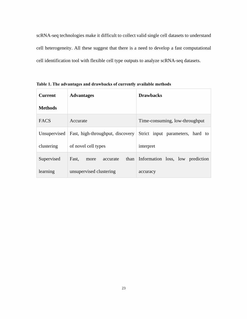
Table 1 shows the advantages and disadvantages of the currently available methods.
Several other problems such as cost [28] and dropouts in gene expression profiling [29] in
23
scRNA-seq technologies make it difficult to collect valid single cell datasets to understand
cell heterogeneity. All these suggest that there is a need to develop a fast computational
cell identification tool with flexible cell type outputs to analyze scRNA-seq datasets.
Table 1. The advantages and drawbacks of currently available methods
Current
Methods
Advantages Drawbacks
FACS Accurate Time-consuming, low-throughput
Unsupervised
clustering
Fast, high-throughput, discovery
of novel cell types
Strict input parameters, hard to
interpret
Supervised
learning
Fast, more accurate than
unsupervised clustering
Information loss, low prediction
accuracy

24
1.4. Major tumor-associated immune cell types
Highly pathogen-specific immune cells produced by the human immune system detect
pathogens and protect the human body against different diseases [30–32]. For example,
tumor infiltrating lymphocytes (TIL) are cells that move from blood into tumors to
eliminate cancer. They are used as prognostic markers for breast cancer including triple-
negative breast cancer (TNBC) and are also associated with reduction in the risk of death
[33]. Another study has also shown that relative risk of distant recurrence of TNBC
decreases by 13% when TILs increase by 10% [34]. Even though there exists evidence
from research that tumors have tolerance over immune cells, a large number of studies have
also shown that tumor-associated immune cells are highly correlated with their tumors and
clinical outcomes [35].
Different proportions of TILs result in different clinical outcomes. Understanding the
heterogeneity of immune cells that are associated with tumors in cancer patients is crucial
and can potentially direct future treatment towards a better post-treatment outcome. Naïve
CD8+ T cells can differentiate into cytotoxic T cells and directly target on tumor cells.
Patients with high expression of CD8+ T cells have better prognosis and better survival
rate in most of the breast cancer subtypes [5, 6]. CD4+ T cells are helper cells that help to
regulate other important defensive cells in human immune system. B cells bind to antigens
and produce specific antibodies for immune response. It has also been shown that B cell
gene expression signatures are well correlated with metastasis free survival in basal-like

25
and human epidermal growth factor receptor 2 (HER2)-enriched cancers [36]. Natural
killer cells, which function in eliminating tumorous and virus-infected cells, are shown to
be accompanied with better prognosis in breast cancer [37]. Other immune cells, such as
macrophages and dendritic cells, also play key roles in fighting cancer and regulating
interactions between tumor and the immune system [38–42]. CD14+ monocytes mainly
differentiate into macrophages and when presenting in a tumor environment the tumor-
associated macrophages usually indicate a poor prognosis [7, 8]. Dendritic cells activate
adaptive immune cells and present antigens. Plasmacytoid dendritic cells, a subtype of
dendritic cells, are associated with worse prognosis [43, 44]. Though most immune cells
have significant impact on tumorigenesis and tumor development, our project focuses on
the 6 cell types mentioned above for modeling the cell subtyping tool due to the fact that
these cells have large datasets publicly available online.
“Cold tumors” are tumors lacking T cell infiltration. Immune checkpoint therapies
have been successfully applied in clinical trials to many cancers [45]; however, “cold
tumors” have low response towards these treatments [46]. It is a great challenge to use
immunotherapy for both research and clinical treatment. In these tumors, however, other
immune cell populations can be observed. By utilizing an immune cell classification model
to determine the immune components of “cold tumors” administered with different
treatments, the therapeutic approaches might be revealed. Therefore, it is necessary to
develop computational models to accurately identify and characterize the key immune cell

26
types from large-scale scRNA-seq immune cell datasets.
1.5. Deep learning algorithms for immune cell subtyping
Deep learning has long been applied in health sciences, such as drug discovery [47],
mutation detection using histopathology images in non-small cell lung cancer [48], and
prediction of protein fold structures [49], among others. In recent years, it has been very
promising for researchers to explore biological mechanisms using the available deep
learning methods. The procedure of immune cell subtyping can also be accelerated with
proper application of current state-of-the-art deep learning methods.
Images are made up of color pixels. By applying a convolutional neural network
(CNN) to an image, the model picks up the high-weighted pixels and tosses the others.
Adjacent pixels are usually well linked with each other and the CNN combines adjacent
pixels with the most important features. In other words, the convolution procedure
decreases the size of the image and extracts the main backbone of the image. This
procedure mimics functions of the animal visual cortex [50]. CNN is considered as a
subclass of deep neural networks from supervised learning, which extracts major features
from input images and performs classification or regression.
Figure 3 shows the comparison between DNN and CNN. The DNN contains an input
layer, an output layer and multiple hidden layers, while the CNN has multiple convolutional
layers other than the layers in DNN. Filters are a set of small pixel grids which usually are
trained to memorize the important features. By performing convolution for an image with

27
a set of filters, the important features on the filters will be highlighted on the image. When
carrying out convolution in CNN, the filters slide around the original input image from top-
left to bottom-right to extract important features. Convolutional layers usually act as feature
extractors and the subsequent DNN network acts as a predictor. Hence, with the extracted
features, the DNN-based models usually show better results than those without feature
extraction.
Figure 3. The hierarchical structure of CNN
CNNs are simply convolutional layers concatenated with DNN. The convolutional layers act as
feature extractors, while DNN makes the prediction. The filters act as sliding windows on each of
the convolutional layers to extract the features and compress original information to generate
feature maps. All feature maps go through the entire DNN for training and in the end the CNN can
be used for making predictions.

28
Due to its excellent performance, CNN has been widely applied in different fields.
Wallach et al. [51] showed that 3D-CNN enabled the neural network to model structure of
proteins without experimental compound activity data. 1-dimensional convolutional neural
network (1D-CNN) is popular for analysis of time series, weather prediction, stock market
prediction and other fields that incorporate sequential data. 1D-CNN was also applied in a
study for creating a bearing fault diagnosis system and demonstrated efficiency with
limited training [52]. In terms of processing RNA sequencing data, CNN has been applied
to pairwise alignment of non-coding RNA for sequence clustering with high accuracy [53].
In terms of scRNA-seq, a recent study also showed that CNN could be used to discover co-
expression gene pairs in scRNA-seq [54].
The gene positional information on chromosomes is critical and should be taken into
consideration when performing analysis based on gene expression level. Studies have
shown that within a genomic neighborhood, genes tend to be expressed similarly [55–57].
In addition, gene positional information has never been applied to analyze genome
sequencing datasets, especially single cell RNA-level data. Thus, considering gene
positional information in CNN may increase its performance.
CNNs often consist of a large network and require long training hours. Hence,
hardware for training CNNs in a time effective way is always needed. Graphics processing
units (GPUs) are special circuits first designed for accelerating image processing. These
29
high-performance and efficient parallel logic architectures have been effective in handling
large blocks of vector and matrix-based mathematical operations. According to the
benchmarking study by Yu et al. [47], with the same trainable parameters and workloads,
normal central processing units (CPUs), which are the core logic structures on our personal
computers, have downsides when working with large batch sizes in deep learning while
GPUs can perform better. CNN has been always designed with complex structures, and
heavy basic mathematical operations such as convolutions and max pooling are executed
during the training phase of the CNN. Using GPU can reduce the overall time for training,
backpropagation, tuning and predicting in deep learning tasks.

30
Chapter 2 Research Motivation, Hypothesis and Aims
2.1. Motivation
Current cell type classification methods have significant limitations, such as excessive
time consumption, low throughput rate of FACS; strict input parameters and high-level
understanding of cell marker genes required for unsupervised clustering; and low accuracy
of current supervised learning methods. In addition, the prevailing unsupervised clustering
methods cannot provide a gold standard for accurately predicting cell types, which leads
to inconsistent results in different studies. Considering only gene expression values for
classifying cell types might be insufficient. Previous study showed that genes were located
on chromosomes with sequential order and expression levels of adjacent gene pairs are
more correlated than others [58], but the gene positional information has not been
considered in most existing models. Genes are aligned in a particular sequence on the
chromosome, so incorporating the gene positional information on chromosomes with gene
expression values will likely increase the accuracy on cell type prediction.
CNN, a powerful model that has been widely applied in computer vision, has also
proved to be useful for scRNA-seq. Hence, our solution for computation-based immune
cell classification is to incorporate 1D-CNN, which has the potential to take chromosome
position information into account with expression values for boosting immune cell type
prediction accuracy.

31
2.2. Hypothesis
We hypothesize that 1D-CNN model incorporating gene positional information on
chromosomes (Chromosome-based neural network, ChrNet) can be learnt from immune-
specific scRNA-seq from human samples collected from well-characterized experiments
to automatically annotate the unlabeled immune cells with higher performance than
currently available methods. The ChrNet model can provide researchers with a standard
procedure for accurately classifying immune cell types. We also expect that the model be
simple, fast, extendable and customizable.
2.3. Research aims
The overall objective of this thesis is to develop a novel deep learning algorithm with
publicly available software for performing immune cell type classification. It has four
specific aims as follows:
Aim 1: To curate immune-specific scRNA-seq datasets from published human studies
and perform data cleaning.
Aim 2: To propose a re-trainable 1D-CNN model that integrates gene positional
information.
Aim 3: To train the model with labeled sets generated from Aim 1 as a reference case,
evaluate the model performance and compare its performance with other supervised
and unsupervised approaches.
Aim 4: Integrate the algorithm into a publicly available Python package.
32
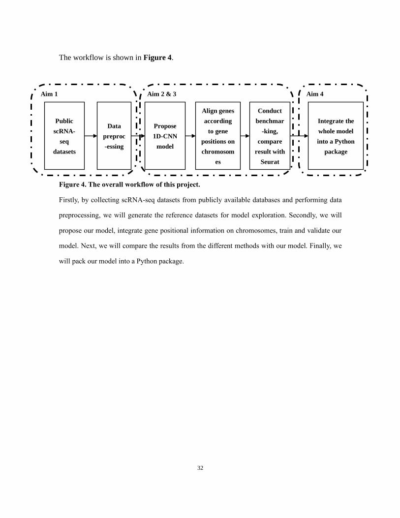
The workflow is shown in Figure 4.
Figure 4. The overall workflow of this project.
Firstly, by collecting scRNA-seq datasets from publicly available databases and performing data
preprocessing, we will generate the reference datasets for model exploration. Secondly, we will
propose our model, integrate gene positional information on chromosomes, train and validate our
model. Next, we will compare the results from the different methods with our model. Finally, we
will pack our model into a Python package.
Public
scRNA-
seq
datasets
Data
preproc
-essing
Propose
1D-CNN
model
Align genes
according
to gene
positions on
chromosom
es
Conduct
benchmar
-king,
compare
result with
Seurat
Integrate the
whole model
into a Python
package
Aim 1 Aim 2 & 3 Aim 4

33
Chapter 3 Materials and Methods
3.1. Data sources
Our datasets are from 3 different studies. The first dataset is well-labeled with immune
cell types and is used for training the model. The other two datasets are without cell type
labels, which will be used as test sets for prediction.
The first dataset [59] includes peripheral blood mononuclear cells (PBMC) of patients
and healthy controls from 13 cases (8 lupus patients, 5 rheumatoid arthritis patients and 2
healthy controls). It includes ~18,000 CD4+ T cells, ~8,600 CD14+ Monocytes, ~4,400 B
cells, ~4,300 CD8+ T cells, ~3,900 Natural Killer cells (NK cells), ~600 Dendritic cells
and ~3,000 Other cells (the cells’ labels that are not in the major cell types mentioned above)
(Table 2). The scRNA-seq data analysis was performed according to the 10x Cell Ranger
pipeline, and the cell type information of all the cells was generated through the pipeline.
This study developed a tool called demuxlet for identifying each cell with the help of
natural genetic variation and detecting droplet consisting of two cells [59]. The cells were
annotated using Seurat software [60].
The second dataset consists of tumor-infiltrating immune cell of breast cancer from
Chung W et al. [27]. This set includes 175 tumor-infiltrating immune cells from 11 Breast
cancer patients (2 luminal A, 1 luminal B, 3 HER2-positive, 5 TNBC) (Table 2). The cells
are not labeled. The study applied the 10xGenomics platform to analyze tumor tissues, and
immune cells were separated from carcinoma using RNA-seq-inferred CNV method. The

34
study focused on immune profiling in a tumor microenvironment.
The last dataset consists of 2,000 immune cells from cord blood and bone marrow
(1000 cells each) from 8 healthy donors in the Human Cell Atlas (HCA) project [61] (Table
2). The cells have not been labeled before. HCA is a database that aims to provide
researchers a collection of scRNA-seq datasets with diverse cell types from different organs,
donors, etc. The HCA project title is, “Census of Immune cells.”
Other information about the participants in these studies, such as sex and age
information, was not available.
3.1.1. Training and validation sets
To train our model for predicting immune cell types using scRNA-seq data, we first
built our training and validation sets using the labeled data set as shown in Table 2. The
limitation of our labeled dataset is that we lacked well-labeled immune datasets, so we used
a labeled set, which includes patients with autoimmune diseases and healthy controls, as a
reference case for training our model. However, we designed the model to be customizable
prior to training. Thus, it is feasible to re-train the model with a labeled data set when it
becomes available. Furthermore, we also explored the model’s generalizability to
unlabeled data set (detailed in next section). In our reference dataset, the labeled set
consisted of 6 major immune cell types: CD8+ T cell, CD4+ T cell, B cell, NK cell, CD14+
Monocyte and Dendritic cell in the model. All other cells not assigned to the immune cell
types were classified as Other. In total, 7 cell types were considered.

35
An algorithm was developed to separate scRNA-seq of approximately 40,000 PBMC
immune cells generated by Kang et al. [59] into the training set and the validation set. This
was done because our reference dataset was unbalanced, that is to say, some cell types had
large numbers of cells while others did not. The validation set was used for evaluating
model performance; therefore, the ability to generate a validation set that is similar to the
training set was important. The splitting algorithm is illustrated in Figure 5. The dataset
was first grouped by their own cell type labels, and from each cell type, 10% of the cells
were collected randomly and then grouped across all cell types to form the validation set.
The rest of the cells were then used as the training set. The gene expression matrices and
cell type labels of the training and validation sets were retained for further training.
Figure 5. The splitting algorithm applied for generating training set and validation set.
We randomly split 10% of the cells in each of the 7 cell types into a validation set and the remaining
90% of the cells into a training set.
36
3.1.2. Test set
The test set included 175 tumor-infiltrating immune cells of breast cancer [27] and
2,000 immune cells from HCA project [61] (Table 2). Since test set was used for prediction
of their cell types using the trained model, we processed the datasets into two expression
matrices for further analysis. With a cancerous dataset and a non-cancerous dataset as the
test set, the generalizability of our model trained on non-cancerous dataset could be further
examined through different conditions. Our Aim 2 was to build a re-trainable classifier for
predicting immune cell types, which could be learned from immune cells with previously
known immune cell types.
The detailed data source information for the training, validation and test set is shown
in Table 2.
37
Table 2. Detailed information of the training set, validation set and test set.
Data
Type
Number of Cells Seque
ncing
Platfo
rm
Source Description Suppleme
ntary
Reference
Labeled
set
(Trainin
g set &
validati
on set)
CD4+ T cell 18,029
HiSeq
2500
Peripheral blood mononuclear
cells from 8 lupus patients, 5
rheumatoid arthritis patients
and 2 healthy controls
sex and age
information
are not
available
[59]
CD14+ Monocyte 8,626
B cell 4,408
CD8+ T cell 4,365
NK cell 3,957
Dendritic cell 676
Other* 3,034
Test set
175 tumor infiltrating
immune cells
HiSeq
2500
11 Breast cancer patients (2
luminal A, 1 luminal B, 3
HER2-positive, 5 Triple
Negative Breast Cancer)
sex and age
information
are not
available
[27]
2000 immune cells
Hiseq
2500/
X
1000 each from cord blood
and bone marrow from 8
healthy donors
sex and age
information
are not
available
[61]

38
3.2. Preprocessing of the datasets
3.2.1 Introduction
Reference genome is constructed by sequencing and combining all chromosomal
fragments from a species, and is a comprehensive representation of the genetic information
in that species [62]. Genes are localized and annotated on the reference genome. Modern
sequencing analysis utilizes the reference genome and aligns the sequenced reads from
experiments to match the genes on the reference genome to carry out expression analysis.
The file containing sequencing results is the fastq file. Gene annotation files contain
information such as gene id, location, description, and others. Different databases have
their own gene id naming, such as ENSEMBL id from Ensembl project [63], and Entrez
ID from the National Center for Biotechnology Information [64], among others. Same gene
id naming format should be applied in every part of the sequence analysis.
3.2.2 Transcripts per kilobase million (TPM)
When comparing the expression levels of samples across different batches or different
library sizes, raw read count cannot be used for direct comparison. Among different
normalization methods, TPM is now becoming more and more popular. Fragments Per
Kilobase Million (FPKM), used for paired-end sequencing, and Reads Per Kilobase
Million (RPKM), used for single-end sequencing, are the normalized values that have been
commonly used in differential analyses in the past [65]. However, RPKM value and FPKM
value would not make good features for direct comparison because the sums of normalized

39
reads are different. Between-sample comparison is possible with TPM values because sums
of all normalized TPM values are the same in different samples.
TPM is implemented according to the formula as follows:
𝑇𝑃𝑀𝑖 =
𝑅𝑖 × 109
𝐺𝐿𝑖
∑𝑅𝑗 × 103
𝐺𝐿𝑗
𝑛𝑗=1
[1]
Where 𝑖 represents the gene 𝑖, 𝑛 stands for number of genes, 𝑅𝑖 stands for the raw
count for gene 𝑖 and 𝐺𝐿𝑖 stands for the gene length for gene 𝑖.
3.2.3 Normalization pipeline applied in our study
The preprocessing step for our study is normalization with TPM. All datasets were
aligned to the same human reference genome build (GRCh37, also known as hg19) and
ENSEMBL ids were the unique ids used in our study. Raw read counts of the datasets were
then converted to TPM values. When gene expression levels are very low, scRNA-seq
sometimes fails to detect the gene. This is called dropout in scRNA-seq. Dropout can occur
due to the stochastic nature of gene expression or may reflect true zeros. Dropout events in
scRNA-seq data analysis can be useful to identify cell types [66]. In our study, since we
are not using gene expression values for differential analysis, dropouts in our datasets can
be considered as dead pixels and will not interfere with the prediction procedure [22].

40
The implementation for converting raw read counts to TPM values is listed in the
following link: https://github.com/Krisloveless/TPM_convertion_tools. We implemented
two versions of the TPM converting tools: one accepts the output from 10xGenomics Cell
Ranger pipeline: https://github.com/10XGenomics/cellranger, and the other converts
results from raw read counts (htseq-count) directly [67]. The second program was
implemented with multithreading to accelerate the speed of the analysis with multicore
CPUs.
After the preprocessing, the dimensions of the datasets remained the same. The
training set contained 38,786 cells, the validation set contained 4,309 cells and the test set
contained 2,175 cells.
3.3. ChrNet: A chromosome-based 1D convolutional neural network
3.3.1 Rationale
The initial purpose of including convolutional layers in neural network-based image
classification is to combine adjacent image regions to reduce the image dimension, because
adjacent regions are often well linked with each other and have similar properties in an
image. CNN is good at extracting information from adjacent pixels on images and has been
proven to significantly improve classification performance in recent years. Some human
genes have been observed to overlap with one another on the same chromosome [68]. If
one of the genes that is overlapping with the other gene has high expression value, the other
gene is likely to also have a high expression value. In other words, adjacent genes on the

41
same chromosome possess similar expression patterns and can be grouped together for
feature extraction. Hence, we adopted this idea to analyze single cell gene expression.
Since adjacent genes on the same chromosome are correlated, they should be grouped
together in order to increase our performance in cell type prediction.
3.3.2 ChrNet architecture and training parameters
We introduce a re-trainable chromosome-based 1D convolutional neural network,
namely, ChrNet. The layout of the ChrNet architecture is shown in Figure 6. All of our
network implementation was based on Keras [69] application programming interface. The
ChrNet model was trained with 2 GeForce GTX 1080ti Nvidia GPUs.
Table 3 lists the tuned parameters when performing the training process. Bolded are
the parameter values with the best model performance (highest accuracy) in the validation
set. With different combinations of the hyperparameters, the parameters in bold with the
highest validation accuracy were selected to construct our model.

42
Figure 6. The layout of ChrNet architecture.
The input features are first selected and aligned to different chromosomes based on their gene
positions. 3 1D-CNN layers are stacked together, followed by a MaxP layer with a BN layer. After
the 3 similar structures, the net goes through two dense layers and then make prediction for the cell
types. Filters indicate the number of filters in that layer and size indicates the size of the filters in
that layer.
Table 3. The list of hyperparameters used to tune the ChrNet.
Hyperparameter Range
filter size in convolutional layer (in 3 3-
stacked layers)
2:4:8,4:8:16,8:16:32,16:32:64,
32:64:128
Maxpooling layer size 2,5,10
Dropout rate 0.2,0.3,0.4,0.5,0.6
Dense layer size 64,128,256,1024
3.3.3 Introduction of major layers in ChrNet
The input layer for ChrNet requires a gene by cell matrix with TPM expression values.
Our input for the ChrNet includes 32,696 genes from 1-22, X and Y human chromosomes,
which has 2 times more genes than SuperCT developed by Xie et al. [22]. Furthermore,
our input accepts TPM values rather than the binary signals used in SuperCT. In the original
gene annotation, genes might overlap with each other. Only the gene with early starting
position was considered to construct our reference dictionary when two given genes were
overlapping. A sorted hg19 [70] bed file was applied to construct a dictionary of genes with

43
gene order information.
The TPM expression values were aligned to each chromosome according to their
linear positions based on the hg19 reference genome. Expression values then went through
3-stacked convolutional (Conv) layers followed by a max pooling (MaxP) 2D layer and a
batch normalization (BN) layer. The filters were used as sliding windows to extract
important features from previous layers. The Conv layers had 4 filters with a size of 3 each
and the MaxP layers had a filter size of 2. Two other similar structures were right after this
layout, in which the number of Conv layers increased to 8 and 16, respectively. Overfitting
is a phenomenon when a model performs well with a training set but when it comes to an
unseen dataset, the model fails to fit the data and has high error rate [71]. On top of each
of the MaxP 2D layers, a dropout layer with a ratio of 0.3 was applied to reduce overfitting
in the training procedure. A dropout rate of 0.3 was employed simply to keep 70% of the
nodes linked to the next layers and tossed the 30% of the nodes randomly. After each of
the MaxP 2D layers, a batch normalization layer was applied for normalizing the
intermediate values to the same degree.
The outputs from these layers were then flattened to fit into fully connected (FC)
layers for further classification. Here, 2 FC layers with 256 neurons were applied to act as
“bottlenecks” for the neural network to extract important features from the convolutional
layers. Two dropout layers with ratio of 0.3 were also applied after each dense layer. All
previous layers ended up with a Rectified Linear Unit (ReLU) activation function, which

44
was used to deal with non-linearity in the dataset. In the end, a softmax activation function
with 7 different classification outcomes was used for prediction, which included: 1) CD8+
T cell; 2) CD4+ T cell; 3) B cell; 4) NK cell; 5) CD14+ monocyte; 6) Dendritic cell and 7)
Other. ReLU and softmax functions are defined as follows:
𝑅𝑒𝐿𝑈(𝑥) = max (𝑥, 0) [2]
𝑆𝑜𝑓𝑡𝑚𝑎𝑥(𝑦 = 𝑘|𝑥) = 𝑒𝑤𝑘
𝑻𝑥+𝑏𝑘
∑ 𝑒𝑤𝑙𝑻𝑥+𝑏𝑙𝐾
𝑙=1
[3]
Where the output is k’s softmax value, K is the number of classes, w is the weight for
input x and b is the bias.
Since we aim to make a re-trainable model, it should be able to accept a totally
different dataset to output different cell types. The output cell types here can be altered if
the model is re-trained with customized cell types for prediction. All layers, filter sizes,
numbers of filters and other parameters can be further tuned for a better output accuracy.
3.3.4 Loss function
A loss function is assigned to a machine learning model for determining how the
model is optimized to gain the best fit with the training dataset.
Sparse_categorical_crossentropy in Keras was applied as a loss function in the training
procedure. “Adam” optimizer with a learning rate of 1e-4 was applied for optimizing the

45
loss. The model’s batch size for training is 40, and was trained with 50 epochs with 900
steps per epoch. The best validation accuracy was saved during the training procedure.
The crossentropy loss function is defined as follows:
𝐿𝑐𝑟𝑜𝑠𝑠𝑒𝑛𝑡𝑟𝑜𝑝𝑦 = −1
𝑀∑ ∑[𝛿(𝑦(𝑚) = 𝑘)log (
𝑒𝑤𝑘𝑻𝑥(𝑚)+𝑏𝑘
∑ 𝑒𝑤𝑙𝑻𝑥(𝑚)+𝑏𝑙𝐾
𝑙=1
)]
𝐾
𝑘=1
𝑀
𝑚=1
[4]
Where M is the number of samples (cells), k is the number of classes (cell types), w
is the weight for input x and b is the bias.
3.3.5 The gene alignment algorithm
Before alignment, we incorporated 32,696 genes from the 1-22, X and Y human
chromosomes based on a sorted hg19 reference genome. ENSEMBL id was applied as a
unique identification for each gene.
After the cell by gene matrix is input to the model, there is a gene alignment procedure
for matching the genes onto the right chromosomes. Routinely, the cell by gene matrix
should be sorted according to the gene labels in the model. However, this is not necessary
to do so for ChrNet. There are a few steps for the alignment. First, the sorted hg19 reference
genome is reconstructed to a gene dictionary with positional information. When iterating
through the genes in a scRNA-seq profile, ChrNet finds whether the gene is in the
constructed gene dictionary or not. If it exists, its expression is then put to the correct

46
positional order in the model; otherwise, the algorithm scans the next gene. After scanning
all genes in that profile, the genes that have no expression values are set to 0 in the model.
After repeating the procedure for all the cell profiles in the matrix, a new curated matrix is
generated. Finally, the curated cell by gene matrix then go through the hidden and output
layers in the CNN model for cell type prediction. The pseudo code of the alignment is
shown in Table 4.
Table 4. Pseudo code for gene alignment algorithm
Gene alignment algorithm
Input: Dataset mat,
N = # of cells,
G = # of genes in the dataset,
mat = N G.
Output: Re-ordered mat’,
G’ = 32,696 genes with pre-defined sequential order in hg19,
mat’ = N G’ = 0.
for i = 1 to N do
for j = 1 to G do
if genename(mat[i][j]) in G’ then
find genename(mat[i][j]) == G’[k]
mat’[i][k] = mat[i][j]
end if
end for
end for
3.3.6 The prediction of an unlabeled single cell
The trained model predicts major tumor-associated immune cell types by sorting
genes to different chromosomes with regards to their linear orders (Figure 7). All RNA

47
expression values from a single cell should be the input to our model, and the goal of our
model is to predict the unknown cell with a specific cell type. After aligning all gene
expressions to each of the chromosomes, the filters act as sliding windows on each of the
chromosomes to carry out the feature extraction and compression of the original
information. The features extracted go through multiple parameter-tuned hidden layers for
dimension transformation and eventually predict a specific cell type shown in the figure.
The model can output the desired cell type as long as the user performs customized training.
Figure 7. The pipeline for prediction.
The trained model accepts an unlabeled cell’s expression matrix and predicts its immune cell types.
The outputs classes include 6 immune cell types: CD8+ T cell, CD4+ T cell, B cell, NK cell and
CD14+ monocyte, Dendritic cell. All other cells not assigned to the immune cell types are classified
as Other cell type. In total there are 7 output cell types. In addition, output cell types can be altered
if the model is re-trained with a different labeled set.

48
3.4. Deep neural network (DNN) and support vector machine (SVM)
model structures
3.4.1 DNN structure
DNN was included for benchmarking the performance with our ChrNet. The same
input with gene alignment process was used. Following Xie et al. method [22], the DNN
had two dense layers with 200 and 100 neurons prior to predict cell types. ReLU activation
function was applied to both dense layers for non-linearity. After each of the dense layers,
a dropout layer with a ratio of 0.4 was added. The last FC layer with outputs of the 7 cell
types was then linked to the last dropout layer with softmax function for activation. Loss
function sparse_categorical_crossentropy was applied to measure the loss. Adam
optimizer with a learning rate of 1e-4 was applied for optimizing the loss. A batch size of
40 and 50 epochs with 900 steps per epoch was applied to our training process, and the
best validation accuracy was saved. The DNN structure applied in our study is shown in
Figure 8.

49
Figure 8. The DNN model applied in our study.
The input cell by gene matrix (a cell with 32,696 genes) first goes through the dense layer with 200
nodes, followed by another dense layer with 100 nodes. After going through a dropout layer with
dropout rate of 0.4, the model then outputs the predicted cell type for a given cell.
3.4.1 SVM structure
SVM was also implemented for comparison with the ChrNet. SVM is a supervised
machine learning method that focuses on finding the hyper planes with maximum distances
towards each of the classes. SVM is illustrated in Figure 9.
50
Figure 9. An illustration of SVM applied in our study.
Two sets of dots (blue and green dots) are shown on the 2D-plane. SVM considers the closest blue
dots and green dots in hyperspace to draw two parallel lines. The solid line in the middle of these
two dash lines is the separation line for blue and green dots.
In our study only linear SVM model was considered. It also received the same input
as our ChrNet but linked directly to 7 different output cell types with linear activation
function and the categorical_hinge loss. Other parameters and training process remained
the same as the previous training procedures of the DNN and the ChrNet. Both models
were trained with 2 GeForce GTX 1080ti Nvidia GPUs.
Linear activation function and hinge loss are defined as follows:
51
𝐿𝑖𝑛𝑒𝑎𝑟(𝑥) = 𝑥 [5]
𝐿ℎ𝑖𝑛𝑔𝑒 = max(0, 1 + 𝑚𝑎𝑥𝑤𝑡𝑥 − 𝑤𝑦𝑥) (𝑡 ≠ 𝑦) [6]
Where t is labels other than y, w is weight and x is the input.
3.5. Performance evaluation
3.5.1 Confusion matrix
A confusion matrix, also known as error matrix, illustrates the overall prediction status
for the model [72]. It is a visualization technique for evaluation of a machine learning
model. The purpose of confusion matrix is to see whether the model is confusing several
classes with each other. Since we had the cell type labels for each of the cell in the
validation set, a confusion matrix was generated to evaluate the performance of a model to
predict the cell type of a given cell.
3.5.2 Cross-validation
Cross-validation is a method for model evaluation with a limited number of data
samples. The reason for using 10-fold cross-validation (10F CV) is that it demonstrates a
lower error variance than conducting only a single evaluation step, providing more
robustness for the evaluation of a given machine learning model [73]. Figure 10 illustrates
the process of 10F CV.

52
Figure 10. An illustration of 10F CV.
The evaluation is performed 10 times. In each time the dataset is separated into 10 equal folds, then
in each evaluation iteration, one of the folds (e.g. the yellow fold) will be the validation set, the rest
of the folds will be the training set for training the model. The model eventually relies on the
validation set for generating the fold accuracy.
10F CV was performed on the reference study dataset (the training and validation sets
in Table 2). Briefly speaking, we equally distributed our labeled cells into 10 equal size
folds, and in each of the validation steps we considered one of the folds to be a validation
set and the rest to be the training set. We repeated this process 10 times and each of the 10
folds was treated as a different validation set for each time. This 10F CV process was
repeated for the 3 supervised learning models (ChrNet, DNN and SVM). To evaluate the
models’ performance in the 10F CV, we used two performance measurements. The first
metric was accuracy (ACC), which is the percentage of the correct predictions in the
labeled set of the 10F CV. The second metric was the F1 score, which is the harmonic mean
of precision and recall of the labeled set in the 10F CV. F1 score is often a good choice
53
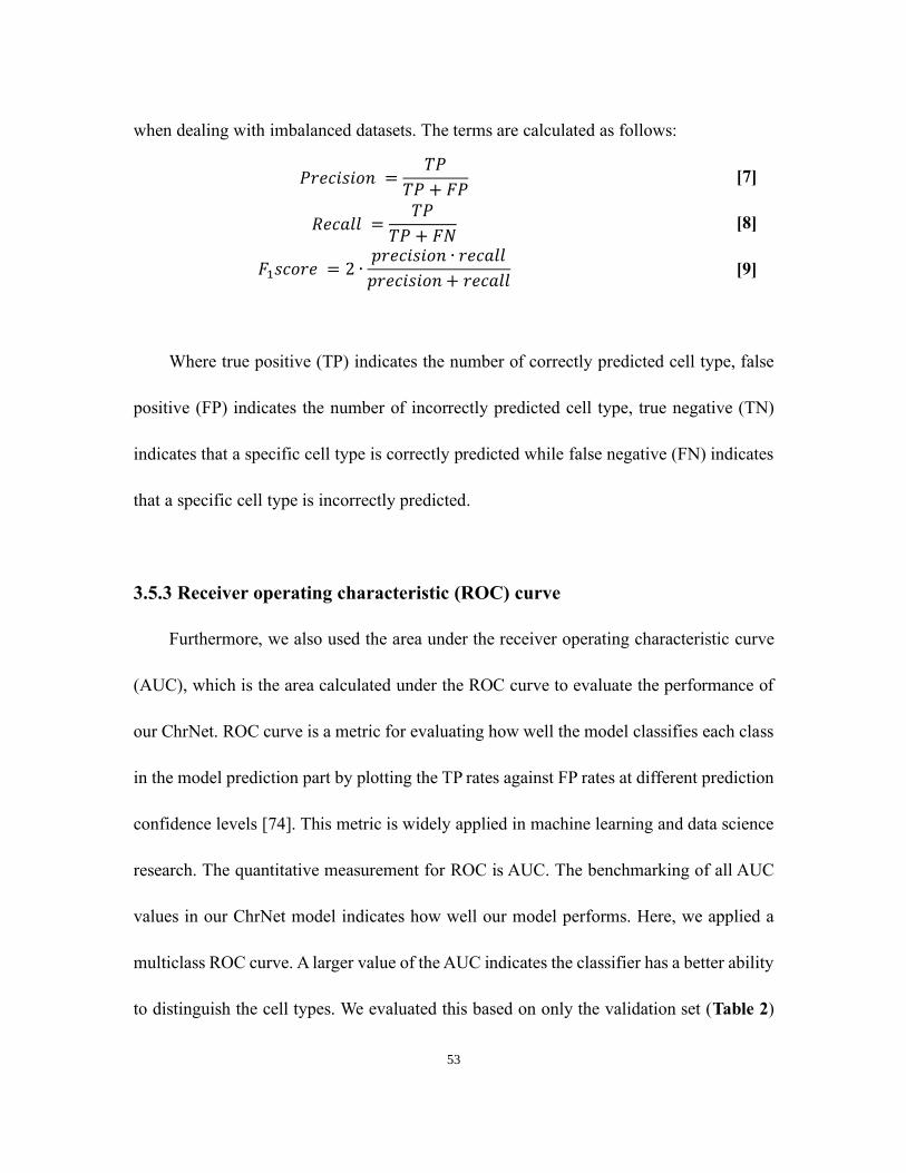
when dealing with imbalanced datasets. The terms are calculated as follows:
𝑃𝑟𝑒𝑐𝑖𝑠𝑖𝑜𝑛 =𝑇𝑃
𝑇𝑃 + 𝐹𝑃 [7]
𝑅𝑒𝑐𝑎𝑙𝑙 =𝑇𝑃
𝑇𝑃 + 𝐹𝑁 [8]
𝐹1𝑠𝑐𝑜𝑟𝑒 = 2 ∙𝑝𝑟𝑒𝑐𝑖𝑠𝑖𝑜𝑛 ∙ 𝑟𝑒𝑐𝑎𝑙𝑙
𝑝𝑟𝑒𝑐𝑖𝑠𝑖𝑜𝑛 + 𝑟𝑒𝑐𝑎𝑙𝑙 [9]
Where true positive (TP) indicates the number of correctly predicted cell type, false
positive (FP) indicates the number of incorrectly predicted cell type, true negative (TN)
indicates that a specific cell type is correctly predicted while false negative (FN) indicates
that a specific cell type is incorrectly predicted.
3.5.3 Receiver operating characteristic (ROC) curve
Furthermore, we also used the area under the receiver operating characteristic curve
(AUC), which is the area calculated under the ROC curve to evaluate the performance of
our ChrNet. ROC curve is a metric for evaluating how well the model classifies each class
in the model prediction part by plotting the TP rates against FP rates at different prediction
confidence levels [74]. This metric is widely applied in machine learning and data science
research. The quantitative measurement for ROC is AUC. The benchmarking of all AUC
values in our ChrNet model indicates how well our model performs. Here, we applied a
multiclass ROC curve. A larger value of the AUC indicates the classifier has a better ability
to distinguish the cell types. We evaluated this based on only the validation set (Table 2)

54
using the trained ChrNet (the trained parameter values can be found in Table 3) from the
10F CV.
3.6. Comparison with unsupervised clustering results
To compare the predicted immune cell types based on the ChrNet with those based on
traditional unsupervised clustering approaches, we followed the online tutorial from Butler
et al. [60] to apply Seurat-based clustering with default parameters to both test sets. Seurat
accepts unlabeled datasets and performs unsupervised clustering. After clustering, the
signature genes for each cluster were extracted for cell type labeling process. In each
dataset, the distribution of the cells and the histogram showing the numbers of cell in each
cluster were plotted. We also integrated our model’s predictions with Seurat’s clusters. In
Seurat’s protocol, marker genes of each clusters were generated with the function
“FindAllMarkers” (find differentially expressed genes). After clustering the cells in the test
sets, we selected genes from the results of “FindAllMarkers” in each cluster for further
examination. Four significant genes in each dataset were selected, and the comparison
between ChrNet’s results and Seurat’s results was illustrated using violin plots.

55
Chapter 4 Results and Discussion
4.1. Processed datasets
The training set contained 38,786 cells and the validation set contained 4,309 cells
with 7 different cell types (-labels). The test set contained 175 tumor-infiltrating immune
cells from breast cancer patients and 2,000 immune cells from healthy donors. All datasets
were normalized with TPM values. All cells in the test sets were not labeled. After applying
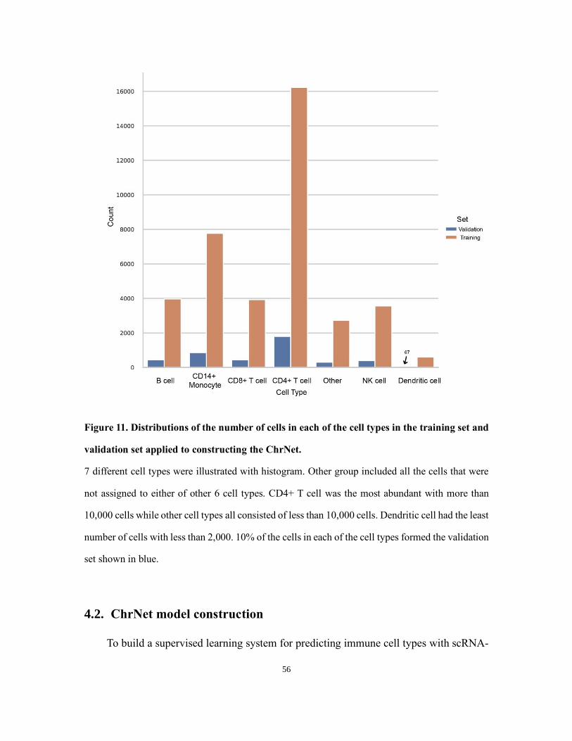
the splitting algorithm mentioned in Figure 5, the distribution for the number of cells in
each of the cell types in the reference case (training and validation set) is shown in Figure
11.
56
Figure 11. Distributions of the number of cells in each of the cell types in the training set and
validation set applied to constructing the ChrNet.
7 different cell types were illustrated with histogram. Other group included all the cells that were
not assigned to either of other 6 cell types. CD4+ T cell was the most abundant with more than
10,000 cells while other cell types all consisted of less than 10,000 cells. Dendritic cell had the least
number of cells with less than 2,000. 10% of the cells in each of the cell types formed the validation
set shown in blue.
4.2. ChrNet model construction
To build a supervised learning system for predicting immune cell types with scRNA-

57
seq, we introduced ChrNet, a re-trainable 1D-CNN model (Figure 7). Our model is capable
of learning not only binary gene expression values (representing presence (coded as 1) or
absence (coded as 0) of gene-specific expression) but also normalized gene expression
levels. The detailed architecture of the model is described in the method section. Briefly
speaking, as shown in Table 2, the ChrNet used immune cell type labels from a previously
published study for training the model. The genes were aligned to the human reference
genome hg19, and feature expression values were extracted from the convolutional layers
to train the model. The model output classes are: 1) CD8+ T cell; 2) CD4+ T cell; 3) B cell;
4) NK cell; 5) CD14+ monocyte, 6) Dendritic cell and 7) Other. Given the expression levels
of an unlabeled cell, the output of the ChrNet is one of the seven cell types we predefined
in the ChrNet. After the model framework was designed, we conducted the selection of
optimized hyper-parameters by experimenting with several combinations of various hyper-
parameters from the filter size in the convolutional layers to the loss function (Table 3).
Different combinations of hyper-parameters resulted in various outcomes, and bolded were
the parameter values with the best model performance (highest accuracy) in the validation
set.
After we trained the model, ChrNet’s performance on our validation set was illustrated
in the format of confusion matrix in Figure 12. The figure shows that the majority of the
cells in each cell type were correctly predicted, although Dendritic cell and Other had a
slightly larger proportion of incorrect predictions. NK cells and CD4+ T cells were more

58
likely to be predicted to be CD8+ T cells, while CD8+ T cells were also likely to be
predicted to be NK cells. This figure suggests that different types of immune cells can
express similar genes and may have overlapping functions.
Figure 12. The confusion matrix of the prediction results for each cell type in the validation
set.

59
The columns of the confusion matrix are the actual cell type labels, while the rows of the matrix
are our model’s prediction results. The colors indicate proportion of cells, where the darker blue
indicates a higher proportion. The diagonal line is the number of cells correctly predicted. The
values outside the parentheses indicate the prediction number and the values inside indicate the
proportion.
4.3. ChrNet performance evaluation
4.3.1 Comparing ChrNet with other classification methods using 10F CV
By benchmarking the three supervised models (ChrNet, DNN and SVM) with 10F
CV, we showed the prediction accuracy of the three models in each of the 10-fold in Figure
13.
Figure 13. The fold-specific accuracy of the three models in the 10-fold cross validation
procedure.
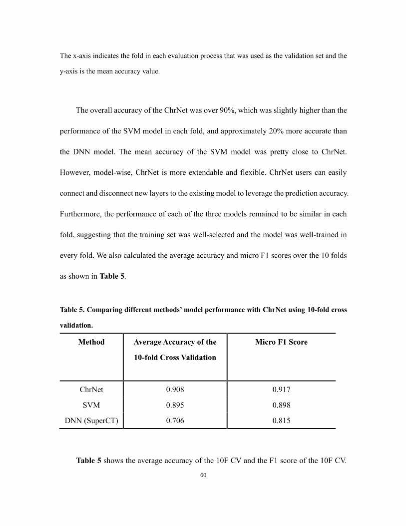
60
The x-axis indicates the fold in each evaluation process that was used as the validation set and the
y-axis is the mean accuracy value.
The overall accuracy of the ChrNet was over 90%, which was slightly higher than the
performance of the SVM model in each fold, and approximately 20% more accurate than
the DNN model. The mean accuracy of the SVM model was pretty close to ChrNet.
However, model-wise, ChrNet is more extendable and flexible. ChrNet users can easily
connect and disconnect new layers to the existing model to leverage the prediction accuracy.
Furthermore, the performance of each of the three models remained to be similar in each
fold, suggesting that the training set was well-selected and the model was well-trained in
every fold. We also calculated the average accuracy and micro F1 scores over the 10 folds
as shown in Table 5.
Table 5. Comparing different methods’ model performance with ChrNet using 10-fold cross
validation.
Method Average Accuracy of the
10-fold Cross Validation
Micro F1 Score
ChrNet 0.908 0.917
SVM 0.895 0.898
DNN (SuperCT) 0.706 0.815
Table 5 shows the average accuracy of the 10F CV and the F1 score of the 10F CV.

61
The average accuracy of the ChrNet reached up to 90%, which was the highest accuracy
among the three models. When considering F1 scores, ChrNet also performed better than
other models. Since F1 score takes precision and recall into consideration for model
evaluation, it is a better metric than cross validation accuracy when comparing multiple
models. For both metrics, ChrNet performed the best among the three models, indicating
that ChrNet is a good and robust model.
4.3.2 Evaluating cell-type specific ChrNet’s performance using ROC curve
After validating that ChrNet has achieved better performance compared to the SVM
and DNN models (Table 5), we visualized multiclass ROCs to examine the performance
for each of the cell types predicted by the trained ChrNet model. The ROC curve is shown
in Figure 14. Overall, all cell types predicted by the ChrNet model had AUC values larger
than 95%, indicating that the model was highly capable of assigning cell types to the cells
without labels.

62
Figure 14. ChrNet-based multiclass ROCs.
ROC curve for each of the cell types was generated with this-type versus not-this-type. For
example, ROC curve of CD4+ T cell is illustrated with CD4+ T cell comparing to all the
other cells.

63
4.4. ChrNet potentially overcame the limitations of the unsupervised
clustering approach
In order to further evaluate the performance of the supervised ChrNet model, we used
the trained ChrNet model to predict the cell types of the 175 breast tumor infiltrating
immune cells and 2,000 immune cells of cord blood and bone marrow (1000 cells each)
from 8 healthy donors from HCA project [61] in the testing set (Table 2). The results are
shown in the next two sections.
4.4.1 Prediction of the tumor infiltrating immune cells: ChrNet vs. the Seurat
unsupervised clustering
As a baseline, we used the state-of-the-art Seurat [60] unsupervised approach to
cluster the 175 cells, which resulted in 5 clusters (Figure 15A). The distribution of the cells
predicted to different cell types using the ChrNet model in each of the clusters is also shown
in Figure 15B. Generally speaking, the ChrNet predicted cell types in cluster 0 were very
diverse, majority of which were CD4+ T cells and CD8+ T cells. Clusters 1 and 2 were
enriched with B cells while clusters 3 and 4 had high proportions of Other and Dendritic
cells.

64
Figure 15. Comparisons of the Seurat unsupervised clustering predictions with our ChrNet’s
predictions of the 175 tumor infiltrating immune cells.
(A) Seurat pipeline was applied to cluster the 175 tumor infiltrating immune cells, and 5 different
clusters were generated. (B) The cell types of the 175 cells were also predicted using our trained
supervised ChrNet. The number of the cells from the different cell types in each of the five clusters
was visualized. The major predicted cell types from our model in Clusters 0-4 are CD4 T+ cell and
CD8 T+ cell, B cell, B cell, Other and Dendritic cell, respectively.
Expression values from the genes selected by Seurat’s “FindAllMarkers” were
illustrated with violin plots shown in Figure 16, which were grouped by the unsupervised
clustering results.
The four different genes were selected based on the top 5 marker genes from each of
the unsupervised clusters Seurat (excluding cluster 3, since cluster 3 is in accordance with
ChrNet’s prediction: Other). Considering the cell type-specific top marker genes selected
by the unsupervised clustering method, which is a crucial step in unsupervised-based cell
labeling procedure, ChrNet also showed great performance. In Figure 16A, CD3D gene,

65
that is relevant to T cell development [75], is the representative marker gene of cluster 0.
Thus, cluster 0 should be labeled as T cells according to Seurat. The major predicted cell
types by our ChrNet with high expression of CD3D are CD8+ T cell and CD4+ T cell,
which is in agreement with Seurat’s clustering results. In Figure 16B we selected MS4A1,
which is the B-Lymphocyte surface antigen [76] and is also one of the canonical genes for
B cells as implemented in Seurat. We can see that both cluster 1 and cluster 2 have higher
expression of MS4A1. MS4A1 is the differentially expressed gene generated by Seurat for
only cluster 1. Therefore, this shows that Seurat may not assign the cells with the same cell
type into the same cell cluster. On the contrary, the predictions by our ChrNet is mainly B
cell for both clusters. Hence, ChrNet proved to have the potential to correct some bias that
the unsupervised clustering method may have made. Previous study showed that ELL3 is
necessary for the proliferation and survival of B cells, and proper cell proliferation and
viability require properly regulated expression level, suggesting that abnormal level of
ELL3 may occur in impaired B cells [77]. In cluster 2 from Figure 16C, most cells highly
expressing ELL3 were labeled as B cell by the ChrNet model which was in accordance
with the results of Seurat. CLEC4C is a protein coding gene related to dendritic cell
developmental lineage pathway [78]. In Figure 16D, the majority of cells with high
expression of CLEC4C were in cluster 4, suggesting that cluster 4 was identified as
Dendritic cells in Seurat. These cells were also predicted to be Dendritic cell by the ChrNet
model.

66
Figure 16. The distributions of the expression levels of the four selected marker genes in the
175 tumor infiltrating immune cells by the unsupervised clustering.
The dot colors represent the predicted cell types using our model ChrNet. The red line indicates the
predicted representative cell type of a given marker gene due to its relatively high expression levels
of the cells in the given cluster. (A) CD3D is predominantly expressed by cells in cluster 0, which
ChrNet mainly predicted the cells as CD8+ T cell and CD4+ T cell. (B) MS4A1 is highly expressed
not only in cluster 1 but also in cluster 2, where most cells are B cell predicted by the ChrNet; (C)

67
ELL3 is mainly expressed in cluster 2 while it is related to B cell; (D) CLEC4C is expressed mostly
in cluster 4.
4.4.2 Prediction of the healthy immune cells: ChrNet vs. the Seurat
unsupervised clustering
The same procedure as the one used for analysis of the tumor infiltrating immune cells
was applied for the 2000 immune cells from the HCA project. The 2000 immune cells were
clustered into 10 different clusters shown in Figure 17A and the distribution of the number
of cells in each of the cell types predicted by the ChrNet in the 10 clusters was shown in
Figure 17B. The results generated by the Seurat and the ChrNet are diverse in each of the
clusters as shown in Figure 17B.
Figure 17. Comparison of the Seurat unsupervised clustering predictions with ChrNet’s
predictions using the 2000 immune cells from the 8 healthy donors.
(A) Seurat was applied to cluster the 2000 immune cells from the 8 healthy donors provided by
HCA project and 10 different clusters were generated. (B) The number of cells in each cell type
predicted by ChrNet in each of the 10 clusters. The cell types predicted in 10 clusters are more
diverse than the previous results from 175 tumor infiltrating immune cells.

68
To further compare the results produced by Seurat and ChrNet, we applied the same
procedure to extract selected marker genes using Seurat; the results are shown in Figure
18. The four different marker genes were selected based on the top 5 marker genes from
each of the 10 unsupervised clusters. In Figure 18A, the signature gene of cluster 0 was
CD3D gene, which is relevant to T cell development as mentioned before. In terms of
results from the ChrNet, a large proportion of cells highly expressing CD3D was shown in
clusters 0, 1 and 4. Other than CD8+ T cell and CD4+ T cell, a large number of CD14+
Monocyte cells were predicted in these 3 clusters. Literature search showed that there exist
TCR+ macrophages [79], that could be an explanation for a large proportion of CD14+
Monocyte cells in cluster 0, 1 and 4. This further demonstrated the advantage of ChrNet
over Seurat: the expression levels of the marker gene from cells predicted to be the same
cell type (according to the marker gene CD3D from Seurat) were relatively high in different
clusters (cells from cluster 0, 1, 4 all have a large number that highly expressing CD3D),
and this might generate bias when performing cell type classification with only Seurat, but
our ChrNet still can accurately predict individual cell types. In Figure 18B the selected
signature gene from Seurat cluster 2 was S100A8, which was shown to be a key regulator
for macrophage inflammatory response [80]. ChrNet predicted that most of S100A8-high
CD14+ Monocytes were mainly in cluster 2, which agreed to Seurat’s results. Marker gene
shown in Figure 18C is CD79B, a B cell antigen receptor coding gene [81], of cluster 3.

69
The majority of B cells predicted by ChrNet were shown to be in cluster 3, which agreed
with Seurat’s result. However, in cluster 3, large amount of CD14+ Monocyte cells were
predicted by ChrNet. Study by Frankenberger et al. showed that CD14+CD16+ monocytes
may highly express CD79B [82], which can be an explanation for the combination of B
cells and CD14+ Monocyte cells in cluster 3 predicted by the ChrNet. In addition, some
cells with high expression of CD79B in cluster 0, 1 and 7 were also predicted to be B cell
by ChrNet, showing that ChrNet can correctly identify cells that are confused by Seurat.
CCL5 gene, one of the major HIV-suppressive factors produced by CD8+ T cells [83], was
the marker gene for cluster 4. In Figure 18D, ChrNet predicted a large proportion of CD8+
T cells in cluster 4. Furthermore, NK cells and some CD14+ Monocyte cells predicted by
ChrNet in cluster 4 also had high expression levels of CCL5.
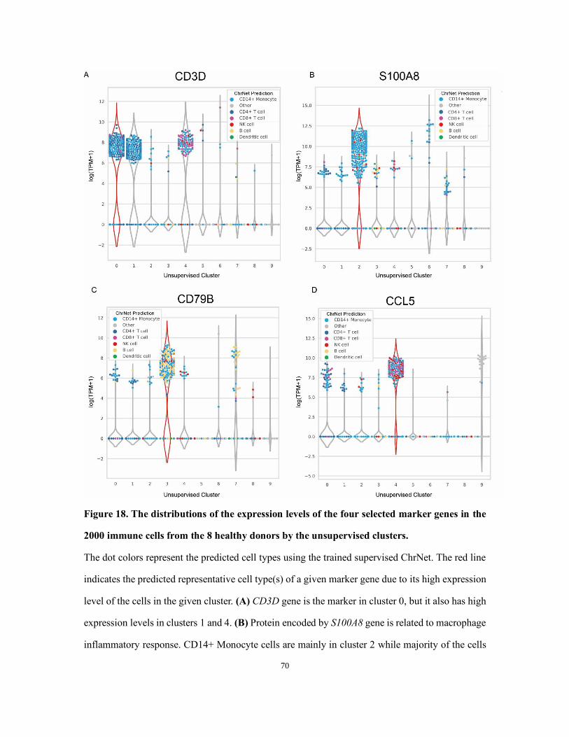
70
Figure 18. The distributions of the expression levels of the four selected marker genes in the
2000 immune cells from the 8 healthy donors by the unsupervised clusters.
The dot colors represent the predicted cell types using the trained supervised ChrNet. The red line
indicates the predicted representative cell type(s) of a given marker gene due to its high expression
level of the cells in the given cluster. (A) CD3D gene is the marker in cluster 0, but it also has high
expression levels in clusters 1 and 4. (B) Protein encoded by S100A8 gene is related to macrophage
inflammatory response. CD14+ Monocyte cells are mainly in cluster 2 while majority of the cells

71
in other clusters with high level expression of S100A8 are CD14+ Monocyte predicted by ChrNet.
(C) CD79B gene is mainly shown in cluster 3. Some cells in clusters 0, 1 and 7 that have high level
expression of CD79B are detected to be B cell by ChrNet. (D) CCL5 gene is the marker gene for
cluster 4. This gene correlates to a large number of CD8+ T cells predicted by ChrNet in cluster 4.
4.5. Software implementation for ChrNet
All our code for the ChrNet algorithm was published in the following link:
https://github.com/Krisloveless/ChrNet. Part of the homepage of the Github is shown
below. All codes were written in Python3. The program can be run under both Linux and
Windows environment. The advantage of our algorithm is that the code can be applied as
references for future algorithm-based research since other researchers can extend or adapt
the algorithm (codes) to their own research needs. A potential extension of our model in
the future might include other cellular information, such as cell size and cell status into our
input. This might elevate the prediction accuracy of our ChrNet. The major modules of the
algorithm tool are introduced below.

72
Figure 19. Homepage of ChrNet online repository.
A homepage illustration of our public repository. We hosted our source code on the website provided
above. The datasets we applied in our study were also made publicly available.
4.5.1 Main.py
Main.py file is the entry point of our whole model. Our program can run with both
CPUs- and GPUs-based machines. The advantage of using CPUs over GPUs is that GPU-
based machines usually have limited size of memory and can often lead to memory limit
error. Moreover, many machines have no GPUs for training the model. During the training
process the program will generate a log for training accuracy and validation accuracy for

73
tuning the model. ‘Run’ function and ‘predict’ function are the major functions for training
the model and predicting cell types of unlabeled cells, respectively. Our model is capable
of training with 1) different reference genomes and 2) different output cell types. To train
with another reference, first, ‘chr_list’ in model.py should be changed to the right
chromosome sizes in the new reference genome. Next, in main.py, the directory for the
reference path to the new reference path should also be changed. If researchers want to
customize the training with another set of cell types, the ‘dict_label’ in data.py should be
changed to the desired output cell types with cell types as keys and the number indices as
values. All of our temporary results are saved in a pickle file, which is a file format to save
a whole data structure object into a storable string, making it easier for loading and
dumping the data. We have also implemented a function to load and save pickle files in
main.py.
4.5.2 Model.py
The entire neural network architecture is written in the model.py file. By tuning
model.py, we can alter the model’s structure for better performance. The model was
implemented as illustrated in Figure 6. Connecting and disconnecting new layers can be
done in this file for altering the model architecture.
4.5.3 Data.py
The major data processing functions are implemented in data.py file. The detailed
description of each of the functions is listed below. However, researchers will not need to

74
alter any parameters in this file in a normal re-training procedure. “Process_reference” is a
function for creating a dictionary for storing the gene names with the starting and ending
positions. It requires the input of the reference genome. “Ten_fold_validation_split” is for
performing a random split of the dataset into 10 different folds for the 10F CV.
“Folding_Generator” is the function for generating the training dataset for the 10F CV. For
example, if input index is “1”, fold 1 will be the validation set and the rest will be combined
as the training set, which are processed to be ready for the model training. “Split_df” is a
function for randomly splitting a percentage of dataset. “Reorder” is a function to prepare
all datasets to be ready for generating the training dataset and is the implementation for the
core gene alignment algorithm. “TrainBatchGenerator” is the main training function for
generating the training set. It can receive an input to set a batch size and to select only top
‘number’ of the input cells for training the model. “Pickle_predict” is the major function
to predict cell types. The output will be saved into a pickle file, and the default output is
the predicted cell types. By changing ‘score=True’, the output will be the score for each
cell type instead of providing the predicted cell type (the cell type with the highest score is
chosen as the predicted cell type). “IG_reorder”, “pickle_predict_with_IG” and
“findMetaFeature” are the functions to first prepare the right format for integrated gradients
(IG) from the cell by gene matrix, then perform prediction and finally find the marker genes
(also called MetaFeatures) for each of the cell types. If a customized training set is used to
train a model with a different set of output, finding MetaFeatures can be still performed. A
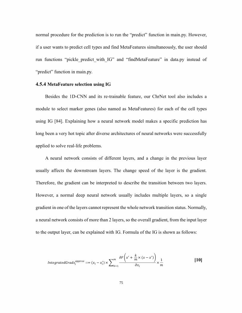
75
normal procedure for the prediction is to run the “predict” function in main.py. However,
if a user wants to predict cell types and find MetaFeatures simultaneously, the user should
run functions “pickle_predict_with_IG” and “findMetaFeature” in data.py instead of
“predict” function in main.py.
4.5.4 MetaFeature selection using IG
Besides the 1D-CNN and its re-trainable feature, our ChrNet tool also includes a
module to select marker genes (also named as MetaFeatures) for each of the cell types
using IG [84]. Explaining how a neural network model makes a specific prediction has
long been a very hot topic after diverse architectures of neural networks were successfully
applied to solve real-life problems.
A neural network consists of different layers, and a change in the previous layer
usually affects the downstream layers. The change speed of the layer is the gradient.
Therefore, the gradient can be interpreted to describe the transition between two layers.
However, a normal deep neural network usually includes multiple layers, so a single
gradient in one of the layers cannot represent the whole network transition status. Normally,
a neural network consists of more than 2 layers, so the overall gradient, from the input layer
to the output layer, can be explained with IG. Formula of the IG is shown as follows:
𝐼𝑛𝑡𝑒𝑔𝑟𝑎𝑡𝑒𝑑𝐺𝑟𝑎𝑑𝑠𝑖𝑎𝑝𝑝𝑟𝑜𝑥 ∷= (𝑥𝑖 − 𝑥𝑖
′) × ∑
𝜕𝐹 (𝑥′ + 𝑘𝑚 × (𝑥 − 𝑥′))
𝜕𝑥𝑖×
1
𝑚
𝑚
𝑘=1
[10]

76
Where m is the number of step size, 𝑖 is the different gene dimension, 𝑥 is the input value
and 𝑥′ is the baseline value.
After cell types of immune cells are predicted by our ChrNet, integrated gradients can
be used for extracting feature attributes among different cells and genes. For a quality
validation of the attribute values, we followed the method proposed by Anupama Jha et al.
[85] for assigning P-value to IG’s output. By extracting the attribute values for each gene
in all samples using the IG algorithm as shown in Table 6, the marker genes for each cell
type in a given scRNA-seq dataset can be identified. The pseudo code is shown below:

77
Table 6. Algorithm for finding significant MetaFeatures
Algorithm for finding significant MetaFeatures
Input: G = [attr(g1), attr(g2), …, attr(gm)],
R = [attr(r1), attr(r2), …, attr(rn)],
m = # of cells in G,
n = # of cells in R,
p = # of genes,
size(G) = m p,
size(R) = n p
Output: Set of significant features F
for i = 1 to p do
SetG = abs([attri(g1), attri(g
2), …, attri(gm)])
SetR = abs([attri(r1), attri(r
2), …, attri(rn)])
p-valuei = one-tailed t-test(SetG, SetR)
T[i] = p-valuei
end for
T’ = Benjamini-Hochberg Correction (T, FWER = 0.05)
for i = 1 to p do
if T’[i] then
F[i] = 1
else
F[i] = 0
end if
end for
Where SetG is all of the cells predicted as a certain cell type being evaluated and SetR
is all of the other cells in the sample. P is the number of genes. The absolute attribute values
for both sets of the cells are obtained before going through a one-tailed t test, with a null
hypothesis that the mean attribute value of SetG is smaller than that of the SetR. Benjamini-
Hochberg multiple testing correction is applied. Only genes with a false discovery rate less

78
than or equal to 0.05 can be considered as the MetaFeatures (significant genes) for that
given cell type. In summary, each cell type will have a set of MetaFeature as its gene
signatures.
This function was originally designed for extracting the signature features in different
cells by explaining the neural network. However, we currently do not have wet lab
validation on the current datasets. We implemented this as a backup for research that
require feature explanations from the neural network. By identifying the MetaFeatures
from the model, we can then apply the algorithm to different diseases such as TNBC to
select the disease-specific gene signatures for each cell type based on the model.

79
Chapter 5 Significance, limitations and future direction
5.1. Significance
In this study, we generated a supervised deep convolutional neural network for
predicting immune cell subtypes with capabilities for re-training, customizable outputs and
a publicly available Python implementation. It should be noted that this study mainly
focused on developing a novel scRNA-seq-based cell classification algorithm and
providing software implementation to accelerate scRNA-seq research. Thus, we applied
real scRNA-seq datasets to test our tool to demonstrate its ability for cell type classification.
We trained the ChrNet model along with other supervised models using the training set and
tested the ChrNet and an unsupervised clustering approach with two test sets. Considering
the lack of well-labeled data set and the limitations of the data set consisting of a mix of
both healthy and disease-specific samples, we evaluated the model’s generalizability to
predict cell types given scRNA-seq from both diseased and healthy individuals. We
demonstrated that the overall performance of the ChrNet is superior to other supervised
models, and is computationally fast and accurate. In addition, ChrNet can not only classify
immune cells but also classify other cell types as long as the model is re-trained to do so.
Without much wet lab experiments, the well-trained model can reliably distinguish
cancer-associated and cell type-specific immune cell signature composition accurately.
Moreover, ChrNet is extendable. The ChrNet architecture is capable of modeling diverse
scRNA-seq sources. With re-trainable structure, researchers can easily extend the model

80
with their own datasets and customize the output cell type according to the aims of their
own projects. Datasets with other variables like survival rate and other cell types can also
be integrated into the ChrNet for improving the prediction accuracy by slightly modifying
the input layers.
It must be noted that supervised models are not better than unsupervised clustering
approaches in all ways. Unsupervised clustering methods are also accurate in identifying
immune cell types when there are large amounts of data, and the supervised model cannot
be trained without the true-labeled cells. Unsupervised clustering methods are capable of
detecting novel cell types while supervised methods are not.
In summary, the proposed ChrNet model provides a reference 1D-CNN classification
model for processing large-scale and high-dimensional scRNA-seq data. As a signature-
specific immune cell classifier that is generalizable, our model can further be applied to
other tumor-associated immune scRNA-seq datasets, even non-immune datasets, for
exploring cellular heterogeneity. Furthermore, our model is extendable and re-trainable
since the users can customize the cell type output according to their own research aims. By
establishing a single-cell level immune subtyping architecture, we expect this will help us
develop fast and timely genomic testing platform for predicting prognosis and other clinical
purposes.
5.2. Limitations
Due to the lack of well-labeled datasets, we were not able to find a better study (the

81
dataset we used is from a study on autoimmune disease which may be too specific) to
generate model weights; however, ChrNet trained with reference dataset showed potential
for predicting immune cells accurately. That is to say, our model was built from
autoimmune disease but used to apply to different conditions. However, since our cell
source was only from a small number of patients, the results from our study may not
represent the whole cancer family. As such, researchers may need to generate their own
datasets for training the model in the future, which is expensive.
From the previous results in Figure 15 and Figure 17, though the overall predictions
from ChrNet were in accordance with the results of Seurat, there existed a mixture of cell
populations in both Figure 15B and Figure 17B. This is one of the drawbacks of the
unsupervised methods Seurat; in other words, further subtyping should only rely on our
model ChrNet. However, we could not validate our test set results with ground truth labels
from wet lab validation. Only differentially expressed genes from each cluster could be
used to validate our ChrNet’s predictions. Moreover, defining a cluster with a single
differentially expressed gene in unsupervised clustering may not be accurate since a cell
type is defined by its cell surface markers. Some cells can have certain surface markers
with low expression of the marker genes. An exploration of the connections between gene
expression and cell surface marker is needed.
Currently scRNA-seq studies are largely relying on unsupervised clustering methods.
However, there is no gold standard for labeling scRNA-seq with only computational
82
methods. Bioinformatics analysis should be aiding the biological discovery with supportive
evidence rather than defining biological facts. Thus, due to this limitation, unsupervised
clustering, if not properly conducted, may produce bias when it is used for labeling cell
types, which may make the entire procedure unreliable. An example of this limitation in
our study was that Seurat produced different clusters with many cells highly expressing
CD3D in Figure 18A. By applying only computational methods, we could not find the
right degree to determine cell types. The solution for this is to generate scRNA-seq datasets
with FACS validation. With validation through wet lab experiments supported by
computational analyses, we may be able to provide a better standard for scRNA-seq
subtyping.
Though the problem of dropouts were omitted in our model, a large percentage of
dropouts can really hinder the feasibility of our model either on the training aspect (cannot
really separate the cell types in training stage and lead to a poor model) or on accuracy
aspect (without enough information to determine the right cell types). Furthermore, in our
study, we do not exactly know what the sequencing qualities for our collected datasets are.
The model only gained around 90% ACC. Currently, the model still has room for
improvements in its performance. Moreover, there are not many methods to compare
against since there are only few published scRNA-seq deep learning methods available
online.
As for the application of our model on cancer diagnosis and prognosis, though ChrNet

83
has achieved high accuracy, it is not feasible to apply clinical immune cell classification
with ChrNet yet, since scRNA-seq experiments are still expensive with respect to time and
cost. Therefore, application of ChrNet should be focused more on research before being
applied as a part of clinical treatment.
5.3. Future directions
Though our study only focuses on immune cells for scRNA-seq-based cell typing, the
model has the potential to be generalized for classifying other cell types using scRNA-seq
datasets, if properly trained. We hope that this can be treated as a reference CNN
architecture for scRNA-seq-based cell classification approach for application to more
diverse cell types.
Furthermore, the gold standard for cell type classification using scRNA-seq should be
further explored. With a gold standard with respect to known cell types, all machine
learning methods can be benchmarked with a reliable baseline. New samples can be
generated to sequence cells after FACS validation, and construct a database that provides
the expression levels of immune cells with their cell type labels in different conditions such
as healthy, breast cancer, lung cancer, etc. As for model performance, other more recently
developed new machine learning models can be implemented to boost its performance.

84
References
1. Marusyk A, Polyak K. Tumor heterogeneity: Causes and consequences. Biochimica et
Biophysica Acta - Reviews on Cancer. 2010;1805:105–17.
2. Altschuler SJ, Wu LF. Cellular Heterogeneity: Do Differences Make a Difference? Cell.
2010;141:559–63.
3. White blood cell - Wikipedia. https://en.wikipedia.org/wiki/White_blood_cell. Accessed
19 Mar 2020.
4. Ward-Hartstonge KA, Kemp RA. Regulatory T-cell heterogeneity and the cancer
immune response. Clin Transl Immunol. 2017;6:e154.
5. Miyashita M, Sasano H, Tamaki K, Chan M, Hirakawa H, Suzuki A, et al. Tumor-
infiltrating CD8+ and FOXP3+ lymphocytes in triple-negative breast cancer: its correlation
with pathological complete response to neoadjuvant chemotherapy. Breast Cancer Res
Treat. 2014;148:525–34.
6. Mahmoud SMA, Paish EC, Powe DG, Macmillan RD, Grainge MJ, Lee AHS, et al.
Tumor-infiltrating CD8+ lymphocytes predict clinical outcome in breast cancer. J Clin
Oncol. 2011;29:1949–55.
7. Al Murri AM, Hilmy M, Bell J, Wilson C, McNicol AM, Lannigan A, et al. The
relationship between the systemic inflammatory response, tumour proliferative activity, T-
lymphocytic and macrophage infiltration, microvessel density and survival in patients with
primary operable breast cancer. Br J Cancer. 2008;99:1013–9.
8. Campbell MJ, Tonlaar NY, Garwood ER, Huo D, Moore DH, Khramtsov AI, et al.
Proliferating macrophages associated with high grade, hormone receptor negative breast
cancer and poor clinical outcome. Breast Cancer Res Treat. 2011;128:703–11.
doi:10.1007/s10549-010-1154-y.
9. Balkwill F, Mantovani A. Inflammation and cancer: Back to Virchow? Lancet. 2001.
10. Gonzalez H, Hagerling C, Werb Z. Roles of the immune system in cancer: From tumor
initiation to metastatic progression. Genes and Development. 2018.

85
11. Gun SY, Lee SWL, Sieow JL, Wong SC. Targeting immune cells for cancer therapy.
Redox Biology. 2019;25.
12. Checkpoint inhibitor - Wikipedia. https://en.wikipedia.org/wiki/Checkpoint_inhibitor.
Accessed 21 Dec 2019.
13. Sanger sequencing - Wikipedia.
https://en.wikipedia.org/wiki/Sanger_sequencing#cite_note-marra-11. Accessed 6 Apr
2020.
14. Massive parallel sequencing - Wikipedia.
https://en.wikipedia.org/wiki/Massive_parallel_sequencing. Accessed 19 Mar 2020.
15. Behjati S, Tarpey PS. What is next generation sequencing? Arch Dis Child Educ Pract
Ed. 2013.
16. Han Y, Gao S, Muegge K, Zhang W, Zhou B. Advanced applications of RNA
sequencing and challenges. Bioinform Biol Insights. 2015;9:29–46.
17. Mason CE, Porter SG, Smith TM. Characterizing multi-omic data in systems biology.
Adv Exp Med Biol. 2014;799:15–38.
18. Hwang B, Lee JH, Bang D. Single-cell RNA sequencing technologies and
bioinformatics pipelines. Experimental and Molecular Medicine. 2018;50.
19. Flow Cytometry (FCM) /FACS | Fluorescence-activated cell sorting (FACS).
https://www.sinobiological.com/flow-cytometry-fcm-facs-fluorescence-activated-cell-
sorting-facs.html. Accessed 19 Mar 2020.
20. Lieberman Y, Rokach L, Shay T. CaSTLe - Classification of single cells by transfer
learning: Harnessing the power of publicly available single cell RNA sequencing
experiments to annotate new experiments. PLoS One. 2018;13:1–16.
doi:10.1371/journal.pone.0205499.
21. Supervised learning - Wikipedia. https://en.wikipedia.org/wiki/Supervised_learning.
Accessed 24 Apr 2020.
22. Xie P, Gao M, Wang C, Zhang J, Noel P, Yang C, et al. SuperCT: a supervised-learning

86
framework for enhanced characterization of single-cell transcriptomic profiles. Nucleic
Acids Res. 2019;47:e48–e48.
23. Lin C, Jain S, Kim H, Bar-Joseph Z. Using neural networks for reducing the dimensions
of single-cell RNA-Seq data. Nucleic Acids Res. 2017;45:1–11.
24. Unsupervised learning - Wikipedia.
https://en.wikipedia.org/wiki/Unsupervised_learning. Accessed 24 Apr 2020.
25. Azizi E, Carr AJ, Plitas G, Cornish AE, Konopacki C, Prabhakaran S, et al. Single-Cell
Map of Diverse Immune Phenotypes in the Breast Tumor Microenvironment. Cell.
2018;174:1293-1308.e36. doi:10.1016/j.cell.2018.05.060.
26. Savas P, Virassamy B, Ye C, Salim A, Mintoff CP, Caramia F, et al. Single-cell profiling
of breast cancer T cells reveals a tissue-resident memory subset associated with improved
prognosis. Nat Med. 2018;24:986–93. doi:10.1038/s41591-018-0078-7.
27. Chung W, Eum HH, Lee HO, Lee KM, Lee HB, Kim KT, et al. Single-cell RNA-seq
enables comprehensive tumour and immune cell profiling in primary breast cancer. Nat
Commun. 2017;8 May:1–12. doi:10.1038/ncomms15081.
28. Wainberg M, Merico D, Delong A, Frey BJ. Deep learning in biomedicine. Nat
Biotechnol. 2018;36:829–38. doi:10.1038/nbt.4233.
29. Haque A, Engel J, Teichmann SA, Lönnberg T. A practical guide to single-cell RNA-
sequencing for biomedical research and clinical applications. Genome Med. 2017;9:1–12.
30. Littman DR, Rudensky AY. Th17 and Regulatory T Cells in Mediating and Restraining
Inflammation. Cell. 2010;140:845–58.
31. Sakaguchi S, Miyara M, Costantino CM, Hafler DA. FOXP3 + regulatory T cells in
the human immune system. Nature Reviews Immunology. 2010;10:490–500.
32. Wing K, Sakaguchi S. Regulatory T cells exert checks and balances on self tolerance
and autoimmunity. Nature Immunology. 2010;11:7–13.
33. Stovgaard ES, Nielsen D, Hogdall E, Balslev E. Triple negative breast cancer–
prognostic role of immune-related factors: a systematic review. Acta Oncol (Madr).

87
2018;57:74–82. doi:10.1080/0284186X.2017.1400180.
34. Loi S, Michiels S, Salgado R, Sirtaine N, Jose V, Fumagalli D, et al. Tumor infiltrating
lymphocytes are prognostic in triple negative breast cancer and predictive for trastuzumab
benefit in early breast cancer: Results from the FinHER trial. Ann Oncol. 2014;25:1544–
50.
35. Pagès F. Tumor-associated immune parameters for personalized patient care. Science
Translational Medicine. 2013;5.
36. Iglesia MD, Vincent BG, Parker JS, Hoadley KA, Carey LA, Perou CM, et al.
Prognostic B-cell signatures using mRNA-seq in patients with subtype-specific breast and
ovarian cancer. Clin Cancer Res. 2014;20:3818–29.
37. Ascierto ML, Idowu MO, Zhao Y, Khalak H, Payne KK, Wang XY, et al. Molecular
signatures mostly associated with NK cells are predictive of relapse free survival in breast
cancer patients. J Transl Med. 2013;11.
38. Medrek C, Pontén F, Jirström K, Leandersson K. The presence of tumor associated
macrophages in tumor stroma as a prognostic marker for breast cancer patients. BMC
Cancer. 2012;12.
39. Sisirak V, Faget J, Gobert M, Goutagny N, Vey N, Treilleux I, et al. Impaired IFN-α
production by plasmacytoid dendritic cells favors regulatory T-cell expansion that may
contribute to breast cancer progression. Cancer Res. 2012.
40. Stewart DA, Yang Y, Makowski L, Troester MA. Basal-like Breast Cancer Cells Induce
Phenotypic and Genomic Changes in Macrophages. Mol Cancer Res. 2012.
41. Tran Janco JM, Lamichhane P, Karyampudi L, Knutson KL. Tumor-infiltrating
dendritic cells in cancer pathogenesis. J Immunol. 2015;194:2985–91.
doi:10.4049/jimmunol.1403134.
42. Markowitz J, Wesolowski R, Papenfuss T, Brooks TR, Carson WE. Myeloid-derived
suppressor cells in breast cancer. Breast Cancer Research and Treatment. 2013;140:13–21.
43. Treilleux I, Blay JY, Bendriss-Vermare N, Ray-Coquard I, Bachelot T, Guastolla JP, et

88
al. Dendritic cell infiltration and prognosis of early stage breast cancer. Clin Cancer Res.
2004;10:7466–74.
44. Palucka K, Coussens LM, O’Shaughnessy J. Dendritic cells, inflammation, and breast
cancer. Cancer Journal (United States). 2013;19:511–6.
45. Ottaviano M, De Placido S, Ascierto PA. Recent success and limitations of immune
checkpoint inhibitors for cancer: a lesson from melanoma. Virchows Archiv. 2019.
46. Bonaventura P, Shekarian T, Alcazer V, Valladeau-Guilemond J, Valsesia-Wittmann S,
Amigorena S, et al. Cold tumors: A therapeutic challenge for immunotherapy. Frontiers in
Immunology. 2019;10 FEB.
47. Wang YE, Wei G-Y, Brooks D. Benchmarking TPU, GPU, and CPU Platforms for Deep
Learning. 2019. http://arxiv.org/abs/1907.10701. Accessed 6 Jan 2020.
48. Coudray N, Ocampo PS, Sakellaropoulos T, Narula N, Snuderl M, Fenyö D, et al.
Classification and mutation prediction from non–small cell lung cancer histopathology
images using deep learning. Nat Med. 2018;24:1559–67.
49. Xu J. Distance-based protein folding powered by deep learning. Proc Natl Acad Sci U
S A. 2019;116:16856–65.
50. Convolutional neural network - Wikipedia.
https://en.wikipedia.org/wiki/Convolutional_neural_network. Accessed 31 Dec 2019.
51. Wallach I, Dzamba M, Heifets A. AtomNet: A Deep Convolutional Neural Network for
Bioactivity Prediction in Structure-based Drug Discovery. 2015;:1–11.
http://arxiv.org/abs/1510.02855.
52. Eren L, Ince T, Kiranyaz S. A Generic Intelligent Bearing Fault Diagnosis System
Using Compact Adaptive 1D CNN Classifier. J Signal Process Syst. 2019;91:179–89.
53. Aoki G, Sakakibara Y. Convolutional neural networks for classification of alignments
of non-coding RNA sequences. Bioinformatics. 2018;34:i237–44.
54. Yuan Y, Bar-Joseph Z. Deep learning for inferring gene relationships from single-cell
expression data. Proc Natl Acad Sci U S A. 2019.

89
55. Oliver B, Parisi M, Clark D. Gene expression neighborhoods. J Biol. 2002;1:4.
http://www.ncbi.nlm.nih.gov/pubmed/12144705%0Ahttp://www.pubmedcentral.nih.gov/
articlerender.fcgi?artid=PMC117247.
56. Michalak P. Coexpression, coregulation, and cofunctionality of neighboring genes in
eukaryotic genomes. Genomics. 2008;91:243–8.
57. Ghanbarian AT, Hurst LD. Neighboring genes show correlated evolution in gene
expression. Mol Biol Evol. 2015;32:1748–66.
58. Arnone JT, Robbins-Pianka A, Arace JR, Kass-Gergi S, McAlear MA. The adjacent
positioning of co-regulated gene pairs is widely conserved across eukaryotes. BMC
Genomics. 2012.
59. Kang HM, Subramaniam M, Targ S, Nguyen M, Maliskova L, McCarthy E, et al.
Multiplexed droplet single-cell RNA-sequencing using natural genetic variation. Nat
Biotechnol. 2018;36:89–94.
60. Butler A, Hoffman P, Smibert P, Papalexi E, Satija R. Integrating single-cell
transcriptomic data across different conditions, technologies, and species. Nat Biotechnol.
2018;36:411–20. doi:10.1038/nbt.4096.
61. Regev A, Teichmann SA, Lander ES, Amit I, Benoist C, Birney E, et al. The human
cell atlas. Elife. 2017;6.
62. Reference genome - Wikipedia. https://en.wikipedia.org/wiki/Reference_genome.
Accessed 8 Jan 2020.
63. Homo sapiens - GRCh37 Archive browser 98.
https://grch37.ensembl.org/Homo_sapiens/Info/Annotation#assembly. Accessed 8 Jan
2020.
64. National Center for Biotechnology Information. https://www.ncbi.nlm.nih.gov/.
Accessed 8 Jan 2020.
65. RPKM, FPKM and TPM, clearly explained | RNA-Seq Blog. https://www.rna-
seqblog.com/rpkm-fpkm-and-tpm-clearly-explained/. Accessed 3 Mar 2020.

90
66. Qiu P. Embracing the dropouts in single-cell RNA-seq analysis. Nat Commun. 2020;11.
67. Anders S, Pyl PT, Huber W. HTSeq-A Python framework to work with high-throughput
sequencing data. Bioinformatics. 2015;31:166–9.
68. Sanna CR, Li WH, Zhang L. Overlapping genes in the human and mouse genomes.
BMC Genomics. 2008;9.
69. Chollet F. Keras: The Python Deep Learning library. KerasIo. 2015.
70. GRCh37 - hg19 - Genome - Assembly - NCBI.
https://www.ncbi.nlm.nih.gov/assembly/GCF_000001405.13/. Accessed 24 Apr 2020.
71. Overfitting - Wikipedia. https://en.wikipedia.org/wiki/Overfitting. Accessed 21 Mar
2020.
72. Confusion matrix - Wikipedia. https://en.wikipedia.org/wiki/Confusion_matrix.
Accessed 21 Mar 2020.
73. Cross-validation (statistics) - Wikipedia. https://en.wikipedia.org/wiki/Cross-
validation_(statistics). Accessed 24 Apr 2020.
74. Receiver operating characteristic - Wikipedia.
https://en.wikipedia.org/wiki/Receiver_operating_characteristic. Accessed 21 Mar 2020.
75. CD3D Gene - GeneCards | CD3D Protein | CD3D Antibody.
https://www.genecards.org/cgi-bin/carddisp.pl?gene=CD3D. Accessed 21 Mar 2020.
76. MS4A1 Gene - GeneCards | CD20 Protein | CD20 Antibody.
https://www.genecards.org/cgi-bin/carddisp.pl?gene=MS4A1. Accessed 21 Mar 2020.
77. Alexander LEMM, Watters J, Reusch JA, Maurin M, Nepon-Sixt BS, Vrzalikova K, et
al. Selective expression of the transcription elongation factor ELL3 in B cells prior to ELL2
drives proliferation and survival. Mol Immunol. 2017;91:8–16.
78. CLEC4C Gene - GeneCards | CLC4C Protein | CLC4C Antibody.
https://www.genecards.org/cgi-bin/carddisp.pl?gene=CLEC4C&keywords=CLEC4C.
Accessed 21 Mar 2020.
79. Chávez-Galán L, Olleros ML, Vesin D, Garcia I. Much more than M1 and M2

91
macrophages, there are also CD169+ and TCR+ macrophages. Front Immunol. 2015;6
MAY:1–15.
80. S100A8 Gene - GeneCards | S100A8 Protein | S100A8 Antibody.
https://www.genecards.org/cgi-bin/carddisp.pl?gene=S100A8. Accessed 22 Mar 2020.
81. CD79B Gene - GeneCards | CD79B Protein | CD79B Antibody.
https://www.genecards.org/cgi-bin/carddisp.pl?gene=CD79B&keywords=CD79b.
Accessed 22 Mar 2020.
82. Frankenberger M, Hofer TPJ, Marei A, Dayyani F, Schewe S, Strasser C, et al.
Transcript profiling of CD16-positive monocytes reveals a unique molecular fingerprint.
Eur J Immunol. 2012.
83. CCL5 Gene - GeneCards | CCL5 Protein | CCL5 Antibody.
https://www.genecards.org/cgi-bin/carddisp.pl?gene=CCL5&keywords=ccl5. Accessed
22 Mar 2020.
84. Sundararajan M, Taly A, Yan Q. Axiomatic attribution for deep networks. 34th Int Conf
Mach Learn ICML 2017. 2017;7:5109–18.
85. Jha A, Aicher JK, Singh D, Barash Y. Improving interpretability of deep learning
models: splicing codes as a case study. bioRxiv. 2019;:700096. doi:10.1101/700096.

92
Appendix
Source code for main.py
1. import os
2. from data import *
3. from model import *
4. from keras.callbacks import ModelCheckpoint,CSVLogger
5. import pickle
6.
7. def save(name,c_object):
8. """Save the weight of TrainBatchGenerator to pkl object.
9. """
10. with open(name,"wb") as saving:
11. pickle.dump(c_object,saving)
12.
13. def load(name):
14. """Load the weight of TrainBatchGenerator from pkl object.
15. """
16. with open(name,"rb") as loading:
17. res = pickle.load(loading)
18. return res
19.
20. def run(training_set_path,reference,weight=None,cpu=False):
21. if cpu:
22. os.environ["CUDA_DEVICE_ORDER"]="PCI_BUS_ID"
23. #force cpu
24. os.environ["CUDA_VISIBLE_DEVICES"]=""
25. # gather the training and validation set.
26. train,validation = TrainBatchGenerator(40,training_set_path,reference)
27. model = ChrNet()
28. # the generators can be save and load for reuse propose.
29. #save("training.pkl",train)
30. #save("validation.pkl",validation)
31. #train = load("training.pkl")
32. #validation = load("validation.pkl")
33. model_checkpoint = ModelCheckpoint("ChrNet.hdf5", monitor="val_acc",verbose=
1,save_best_only=True)
34. csv_logger = CSVLogger("training_ChrNet.log")
35. model.fit_generator(train,steps_per_epoch=900,epochs=50,callbacks=[csv_logge
r,model_checkpoint],validation_data=validation,validation_steps=200)

93
36.
37. def predict(file,model_path,reference,outname,cpu=False):
38. if cpu:
39. os.environ["CUDA_DEVICE_ORDER"]="PCI_BUS_ID"
40. #force cpu
41. os.environ["CUDA_VISIBLE_DEVICES"]=""
42. model = ChrNet(model_path)
43. pickle_predict(file,reference,model,outname)
44.
45. if __name__ == '__main__':
46. run("./dataset/training_tpm.tsv","./reference/hg19.sorted.bed")
47. #predict(".dataset/testing_tpm.tsv","./pre_trained/ChrNet.hdf5","./reference
/hg19.sorted.bed","ChrNet_prediction",cpu=True)
Source code for model.py
1. from keras.models import *
2. from keras.layers import *
3. from keras.optimizers import *
4. from keras.utils.vis_utils import plot_model
5.
6. def ChrNet(pretrained_weights = None):
7. input_sequence = ['1', '2', '3', '4', '5', '6', '7', '8', '9', '10', '11', '
12', '13', '14', '15', '16', '17', '18', '19', '20', '21', '22', 'X', 'Y']
8. # here chr_list is initalized according to hg19.sorted.bed
9. # gene size is here; if using another version of reference please change the
size of each chromosome
10. chr_list = [3203, 2205, 1730, 1364, 1658, 1636, 1431, 1335, 1239, 1267, 1921
, 1718, 612, 1099, 1075, 1486, 1873, 645, 2031, 829, 462, 703, 1062, 112]
11. multi_inputs = [Input((i,1)) for i in chr_list]
12. tmp = [None] * len(input_sequence)
13. for k,v in enumerate(tmp):
14. tmp[k] = Conv1D(4,3,activation="relu",padding="same",name="Conv1_{}".for
mat(input_sequence[k]))(multi_inputs[k])
15. for k,v in enumerate(tmp):
16. tmp[k] = Conv1D(4,3,activation="relu",padding="same",name="Conv2_{}".for
mat(input_sequence[k]))(v)
17. for k,v in enumerate(tmp):
18. tmp[k] = Conv1D(4,3,activation="relu",padding="same",name="Conv3_{}".for
mat(input_sequence[k]))(v)
19. for k,v in enumerate(tmp):
20. tmp[k] = Dropout(0.3)(v)

94
21. for k,v in enumerate(tmp):
22. tmp[k] = MaxPooling1D(2)(v)
23. for k,v in enumerate(tmp):
24. tmp[k] = BatchNormalization()(v)
25. for k,v in enumerate(tmp):
26. tmp[k] = Conv1D(8,3,activation="relu",padding="same",name="Conv4_{}".for
mat(input_sequence[k]))(v)
27. for k,v in enumerate(tmp):
28. tmp[k] = Conv1D(8,3,activation="relu",padding="same",name="Conv5_{}".for
mat(input_sequence[k]))(v)
29. for k,v in enumerate(tmp):
30. tmp[k] = Conv1D(8,3,activation="relu",padding="same",name="Conv6_{}".for
mat(input_sequence[k]))(v)
31. for k,v in enumerate(tmp):
32. tmp[k] = Dropout(0.3)(v)
33. for k,v in enumerate(tmp):
34. tmp[k] = MaxPooling1D(2)(v)
35. for k,v in enumerate(tmp):
36. tmp[k] = BatchNormalization()(v)
37. for k,v in enumerate(tmp):
38. tmp[k] = Conv1D(16,3,activation="relu",padding="same",name="Conv7_{}".fo
rmat(input_sequence[k]))(v)
39. for k,v in enumerate(tmp):
40. tmp[k] = Conv1D(16,3,activation="relu",padding="same",name="Conv8_{}".f
ormat(input_sequence[k]))(v)
41. for k,v in enumerate(tmp):
42. tmp[k] = Conv1D(16,3,activation="relu",padding="same",name="Conv9_{}".f
ormat(input_sequence[k]))(v)
43. for k,v in enumerate(tmp):
44. tmp[k] = Dropout(0.3)(v)
45. for k,v in enumerate(tmp):
46. tmp[k] = MaxPooling1D(2)(v)
47. for k,v in enumerate(tmp):
48. tmp[k] = BatchNormalization()(v)
49. for k,v in enumerate(tmp):
50. tmp[k] = Flatten()(v)
51. for k,v in enumerate(tmp):
52. tmp[k] = Model(inputs=multi_inputs[k],outputs=tmp[k])
53. combined = concatenate([i.output for i in tmp])
54. combined = Dense(256,activation="relu",name="combined1")(combined)
55. combined = Dropout(0.3)(combined)

95
56. combined = Dense(256,activation="relu",name="combined2")(combined)
57. combined = Dropout(0.3)(combined)
58. combined = Dense(7,activation="softmax",name="combined3")(combined)
59. model = Model(inputs=[i.input for i in tmp],outputs=combined)
60.
61. model.compile(optimizer = Adam(1e-
4), loss = 'sparse_categorical_crossentropy', metrics = ['accuracy'])
62.
63. if(pretrained_weights):
64. model.load_weights(pretrained_weights,by_name=True)
65.
66. return model
67.
68. if __name__ == '__main__':
69. model = ChrNet()
70. model.summary()
71. plot_model(model, to_file="model_plot.png", show_shapes=True, show_layer_nam
es=True)
Source code for data.py
1. import numpy as np
2. import os
3. import pandas as pd
4. from keras.utils import Sequence
5. from sklearn.utils import shuffle
6. import pickle
7. from keras.utils import to_categorical
8. import random
9. from IntegratedGradients import *
10. from itertools import chain
11. from scipy import stats
12. from statsmodels.stats.multitest import multipletests
13.
14. input_sequence = ['1', '2', '3', '4', '5', '6', '7', '8', '9', '10', '11', '12',
'13', '14', '15', '16', '17', '18', '19', '20', '21', '22', 'X', 'Y']
15. # dict_label can be changed here for customized training
16. dict_label = {"B cells":0,"CD14+ Monocytes":1,"CD4+ T cells":2,"CD8+ T cells":3,
"Dendritic cells":4,"NK cells":5,"Other":6}
17.
18. def out_label():
19. """Return the inital labels.

96
20. """
21. return dict_label
22.
23. def process_reference(reference_bed):
24. """Process the reference bed file, if altered also please
25. change the model.py chr_list, input a reference such as
26. hg19.sorted.bed.
27. """
28. res = {}
29. with open(reference_bed,"r") as f:
30. for i in f.readlines():
31. container = i.rstrip().split("\t")
32. if container[0] not in res.keys():
33. tmp = []
34. tmp.append(container[1])
35. res[container[0]] = tmp
36. else:
37. res[container[0]].append(container[1])
38. return res
39.
40. class Generator(Sequence):
41. """A generator for providing objects for model.fit_generator
42. """
43. # Class is a dataset wrapper for better training performance
44. def __init__(self,x_set,y_set,validation=False,batch_size=34):
45. self.x,self.y = x_set,np.array(y_set)
46. self.batch_size = batch_size
47. self.indices = np.arange(self.x[0].shape[0])
48. self.validation = validation
49.
50. def __len__(self):
51. return int(np.floor(self.x[0].shape[0] / self.batch_size))
52.
53. def __getitem__(self,idx):
54. inds = self.indices[idx * self.batch_size:(idx + 1) * self.batch_size]
55. batch_x = [self.x[i][inds].reshape(self.batch_size,-
1,1) for i in range(len(self.x))]
56. batch_y = self.y[inds]
57. return batch_x, batch_y
58.
59. def on_epoch_end(self):

97
60. if not self.validation:
61. np.random.shuffle(self.indices)
62.
63. def Ten_fold_validation_split(training_path):
64. """Split a tsv file with gene by sample to 10 folds and
65. save with pickle.
66. """
67. print("reading tsv")
68. df = pd.read_csv(training_path,sep="\t",header=0,index_col=0)
69. df = shuffle(df)
70. samples = len(df.index)
71. batch_size = int(np.floor(samples / 10))
72. for i in range(10):
73. out = df.iloc[i*batch_size:(i+1)*batch_size,:]
74. out.to_pickle("fold_{}.pkl".format(i))
75.
76. def folding_Generator(index,batch_size,reference_bed,categorical=False):
77. """Convert fold pickles in the current directory for fit_generator.
78. """
79. training = []
80. validation = None
81. for i in range(10):
82. out = pd.read_pickle("fold_{}.pkl".format(i))
83. if i == int(index):
84. validation = out
85. else:
86. training.append(out)
87. training = pd.concat(training)
88. print("processing labels")
89. dict_label = out_label()
90. print("processing reference")
91. dict_reference = process_reference(reference_bed)
92. print("reordering")
93. t_x,t_y = reorder(training,dict_reference,dict_label)
94. v_x,v_y = reorder(validation,dict_reference,dict_label)
95. if categorical:
96. t_y = to_categorical(t_y)
97. v_y = to_categorical(v_y)
98. return Generator(t_x,t_y,validation=False,batch_size=batch_size),Generator(v
_x,v_y,validation=True,batch_size=batch_size)
99.

98
100. def split_df(df,percentage=0.9):
101. """Random splitting dataframe according to a percentage.
102. """
103. table = {}
104. gb = df.groupby(df.index)
105. unique = set(df.index)
106. for i in unique:
107. table[i] = gb.get_group(i)
108. training = []
109. validation = []
110. for i in unique:
111. index = np.floor(percentage * table[i].shape[0]).astype(np.int64)
112. training.append(table[i].iloc[:index,:])
113. validation.append(table[i].iloc[index:,:])
114. training_res = pd.concat(training)
115. validation_res = pd.concat(validation)
116. indices = random.sample(range(training_res.shape[0]),training_res.shape[0])
117. training_res = training_res.iloc[indices,:]
118. indices = random.sample(range(validation_res.shape[0]),validation_res.shape[
0])
119. validation_res = validation_res.iloc[indices,:]
120. return training_res,validation_res
121.
122. def reorder(df,dr,dl,test=False):
123. """Reordering dataframe to fit in fit_generator. If test, the
124. will output the original labels, else will output the labels
125. according to dict_label's value(int).
126. """
127. samples = df.shape[0]
128. x_set = [np.zeros((samples,len(dr[i]))) for i in input_sequence]
129. y_set = []
130. for h,i in enumerate(input_sequence):
131. for k,j in enumerate(dr[i]):
132. if j in df.columns:
133. x_set[h][:,k] = np.copy(df[j])
134. if test == True:
135. for i in df.index:
136. y_set.append(i)
137. return x_set,y_set
138. for i in df.index:

99
139. y_set.append(dl[i])
140. return x_set,y_set
141.
142. def TrainBatchGenerator(batch_size,training_path,reference_bed,categorical=False
,number=None):
143. """Initalize the parameters with batch_size, dataframe directory,
144. reference_bed directory. If categorical, the value is converted to
145. y to one-hot vectors. If number, the first `number` of set inputted
146. will be applied to fit_generator. Input training file should be
147. a tsv file where rows should be cells and columns should be genes
148. , first column indicating the cell type and first row indicating gene
149. name (Ensembl ID).
150. """
151. print("processing labels")
152. dict_label = out_label()
153. print("reading tsv")
154. training_set = pd.read_csv(training_path,sep="\t",header=0,index_col=0)
155. #training_set,df_mean = pre_processing(training_set)
156. if number is not None:
157. training_set = training_set.iloc[:int(number),]
158. print("processing reference")
159. dict_reference = process_reference(reference_bed)
160. #need to perform validation split manually
161. print("splitting df")
162. df_train,df_validation = split_df(training_set,percentage=0.9)
163. print("reordering")
164. t_x,t_y = reorder(df_train,dict_reference,dict_label)
165. v_x,v_y = reorder(df_validation,dict_reference,dict_label)
166. if categorical:
167. t_y = to_categorical(t_y)
168. v_y = to_categorical(v_y)
169. return Generator(t_x,t_y,validation=False,batch_size=batch_size),Generator(v
_x,v_y,validation=True,batch_size=batch_size)
170.
171. def pickle_predict(df,reference_bed,model,out_name,dataframe=False,score=False,t
est=False):
172. """Predict with the trained model. The file will be named
173. `out_name`. If dataframe, the prediction will be output of
174. csv and a pickle file (both containing the same result, a
175. pickle file for a quicker input to python). If score,
176. the prediction score will be provided. If test, the real labels

100
177. will be provided. Input file should be a tsv file or pkl a pkl
178. that is holding a pandas dataframe where rows should be cells
179. and columns should be genes.
180. """
181. print("processing labels")
182. dict_label = out_label()
183. print("reading tsv")
184. t_y = None
185. if df.endswith("tsv"):
186. out = pd.read_csv(df,sep="\t",header=0,index_col=0)
187. elif df.endswith("pkl"):
188. out = pd.read_pickle(df)
189. else:
190. raise Exception("Not a valid tsv or pkl file")
191. print("processing reference")
192. dict_reference = process_reference(reference_bed)
193. t_x,t_y = reorder(out,dict_reference,dict_label,test=test)
194. batch_x = [t_x[i].reshape(t_x[i].shape[0],-1,1) for i in range(len(t_x))]
195. res = model.predict_on_batch(batch_x)
196. if dataframe:
197. df_res = pd.DataFrame(res)
198. df_res.columns = [i[0] for i in dict_label.items()]
199. df_res.index = out.index
200. df_res.to_csv(out_name + ".csv")
201. df_res.to_pickle(out_name + ".pkl")
202. else:
203. if score:
204. with open(out_name,"wb") as w:
205. pickle.dump({"true_label":t_y,"predict_label":res},w)
206. else:
207. res_index = [np.argmax(i) for i in res]
208. with open(out_name,"wb") as w:
209. pickle.dump({"true_label":t_y,"predict_label":res_index},w)
210.
211. def IG_reorder(input_batch):
212. """A function for reordering into the right reorder
213. that is accepted by intergrated gradients.
214. """
215. out = []
216. samples = input_batch[0].shape[0]
217. for i in range(samples):

101
218. tmp = []
219. for j in input_batch:
220. tmp.append(j[i,:,:])
221. out.append(tmp)
222. return out
223.
224. def pickle_predict_with_IG(df,reference_bed,model,out_name):
225. """Prediction with intergrated gradients. Input should be a
226. tsv or a pkl that is holding a pandas dataframe. Output csv
227. is the prediction result, while pkl file is the attribute of
228. different cell types.
229. """
230. print("processing labels")
231. dict_label = out_label()
232. print("reading csv")
233. t_y = None
234. if df.endswith("tsv"):
235. out = pd.read_csv(df,sep="\t",header=0,index_col=0)
236. elif df.endswith("pkl"):
237. out = pd.read_pickle(df)
238. else:
239. raise Exception("Not a valid tsv or pkl file")
240. print("processing reference")
241. dict_reference = process_reference(reference_bed)
242. t_x,t_y = reorder(out,dict_reference,dict_label,test=True)
243. batch_x = [t_x[i].reshape(t_x[i].shape[0],-1,1) for i in range(len(t_x))]
244. res = model.predict_on_batch(batch_x)
245. ig = integrated_gradients(model)
246. res_index = [np.argmax(i) for i in res]
247. IG_batch = IG_reorder(batch_x)
248. attribute = [ig.explain(i) for i in IG_batch]
249. barcode = t_y
250. pl = res_index
251. value = pd.DataFrame(np.array(barcode,dtype=object).reshape(-1,1))
252. prediction = pd.DataFrame(np.array(pl,dtype=object).reshape(-1,1))
253. conout = pd.concat([value,prediction],axis=1)
254. conout.columns = ["","Cluster"]
255. name = os.path.split(out_name)[1].split(".")[0]
256. # csv output here
257. conout.to_csv("{}.csv".format(name),index=False)
258. # resout is sample x gene

102
259. genes = [i.shape[0] for i in attribute[0]]
260. resout = np.zeros((len(attribute),sum(genes)))
261. resout = pd.DataFrame(resout)
262. tmp = [dict_reference[i] for i in input_sequence]
263. colnames = [i for i in chain(*tmp)]
264. resout.columns = colnames
265. resout.index = barcode
266. for i in range(len(attribute)):
267. tmp = [j[0] for j in chain(*(attribute[i]))]
268. resout.iloc[i,] = tmp
269. resout.to_pickle("{}_attribute.pkl".format(out_name))
270.
271. def findMetaFeature(pkl,cluster_csv,out_name,classes=len(dict_label)):
272. """Find the metafeatures from the model in each of the
273. cell types. Input should be output files from
274. pickle_predict_with_IG. classes is the number of class
275. for the model, default is 7.
276. """
277. data = pd.read_pickle(pkl)
278. reference = pd.read_csv(cluster_csv,header=0,index_col=0)
279. label = reverse_label()
280. for i in range(classes):
281. outname = "".join(label[i].split(" "))
282. current_index = reference[reference["Cluster"] == i].index
283. none_index = reference[reference["Cluster"] != i].index
284. G_set = abs(data.loc[current_index])
285. R_set = abs(data.loc[none_index])
286. gene_name_all = data.columns
287. MetaName = []
288. Pval = []
289. for j in range(G_set.shape[1]):
290. G_set_single = G_set.iloc[:,j].tolist()
291. R_set_single = R_set.iloc[:,j].tolist()
292. if G_set_single == R_set_single:
293. continue
294. P_out = stats.ttest_ind(G_set_single,R_set_single, equal_var=True).p
value
295. if np.isnan(P_out):
296. continue
297. MetaName.append(gene_name_all[j])
298. # two side to one side check for null hypothesis

103
299. P_out = P_out / 2
300. Pval.append(P_out)
301. if len(Pval) == 0:
302. continue
303. p_adjusted = multipletests(Pval, alpha=0.05, method='fdr_bh')
304. p_adj_value = p_adjusted[1]
305. sig = {}
306. #print(label[i],":",len(p_adjusted[0][p_adjusted[0]==True]))
307. for j in range(len(p_adjusted[0])):
308. if p_adjusted[0][j]:
309. sig[MetaName[j]] = p_adj_value[j]
310. with open("{}_{}_Meta.pkl".format(out_name,outname),"wb") as pkl:
311. pickle.dump(sig,pkl)
312.
313. if __name__ == '__main__':
314. pass