a novel approach of three-dimensional hybrid grid ... · a novel approach of three-dimensional...

Comput. Methods Appl. Mech. Engrg. 192 (2003) 4147–4171

www.elsevier.com/locate/cma

A novel approach of three-dimensional hybridgrid methodology: Part 1. Grid generation

Yao Zheng *, Meng-Sing Liou

NASA Glenn Research Center, MS 5-11, 21000 Brookpark Road, Cleveland, OH 44135, USA

Received 13 August 2001; received in revised form 22 April 2003; accepted 21 May 2003

Abstract

We propose a novel approach of three-dimensional hybrid grid methodology, the DRAGON grid method in the

three-dimensional space. The DRAGON grid is created by means of a Direct Replacement of Arbitrary Grid Over-

lapping by Nonstructured grid, and is structured-grid dominated with unstructured grids in small regions. The

DRAGON grid scheme is an adaptation to the Chimera thinking. It is capable of preserving the advantageous features

of both the structured and unstructured grids, and eliminates/minimizes their shortcomings. In the present paper, we

describe essential and programming aspects, and challenges of the three-dimensional DRAGON grid method, with

respect to grid generation. We demonstrate the capability of generating computational grids for multi-components

complex configurations.

� 2003 Elsevier B.V. All rights reserved.

Keywords: Computational fluid dynamics; Grid generation; Hybrid grid

1. Introduction

An effective CFD system for routine calculation of engineering problems, usually involving complex

geometry, must possess certain features such as: (1) fast turnaround and (2) accurate and reliable solution.

The first point, encompassing both the human and machine efforts, entails a short setup time for calcu-

lation, minimal memory requirement, and efficient and robust solution algorithm. The second point re-

quires a judicious choice of discretization procedure. Choice of grid methodologies will greatly influencewhether the above two criteria are met satisfactorily. In fact, the bulk of human effort, essentially involved

in the grid generation, has been seen no significant reduction over the years, while on the contrary the

machine effort has been dramatically reduced due to the incredible progress in microchips technology.

A propulsion system is an example of complex geometry, involving many separate geometrical entities

(multi-connected domain) with odd shapes and sharp turns. This topology creates challenges to grid

* Corresponding author. Present address: Center for Engineering and Scientific Computation, and College of Computer Science,

Zhejiang University, Hangzhou, Zhejiang 310027, PR China.

E-mail addresses: [email protected], [email protected] (Y. Zheng), [email protected] (M.-S. Liou).

0045-7825/$ - see front matter � 2003 Elsevier B.V. All rights reserved.

doi:10.1016/S0045-7825(03)00385-2

mail to: [email protected],

4148 Y. Zheng, M.-S. Liou / Comput. Methods Appl. Mech. Engrg. 192 (2003) 4147–4171

generation, especially for viscous flow calculations. For a typical three-dimensional flow calculation for apractical engineering device, the time spent in generating a grid is about two thirds of the total simulation

effort, resulting in a serious bottleneck in the entire design/analysis cycle, see [41] for example. Hence, grid

generation continues to be the pacing technology for a practical CFD analysis and is the area where sig-

nificant payoff can be realized. Furthermore, high quality grids for encompassing viscous regions are es-

sential to yielding an accurate and efficient solution.

During the past decades, both structured and unstructured grid techniques have been extensively de-

veloped and applied to solution of various engineering problems. To deal with situations in which complex

geometry imposes considerable constraints and difficulties in generating grids, composite structured gridschemes and unstructured grid schemes currently are the two mainstream approaches.

The Chimera grid scheme [2,8,39] and similar schemes [1,7,9], using overset grids to resolve complex

geometries or flow features, are generally classified into the composite structured grid category. Overset

grids allow structured grids to be used with good quality, such as orthogonality and smoothness, and with

ease to control grid spacing in viscous layers. While being used regularly for flows about complex con-

figuration [8,39], it has also been used to analyze flows over objects in relative motion [10,28]. Furthermore,

overset grids can be employed as a solution adaptation procedure [4,17,27]. However, the nonconservative

interpolations to update variables in the overlapped region, without strict satisfaction of the governingequations, can give rise to spurious solutions, especially through regions of sharp gradients [19,43].

Our experiences have indicated that the interpolation error can become globally significant if numerical

fluxes are not fully conserved, in particular when a discontinuity runs through the interpolated region. Also,

this error can be strongly affected by the underlying flux schemes, such as central vs. upwind schemes. It

must be noted that conservative interpolation schemes in two dimensions [29,44] have been shown to be

relatively easy to implement. Extension to three dimensions for irregular polyhedra, however, is not all that

straightforward. Even if the three-dimensional conservative interpolation proves to be feasible, a funda-

mental difficulty exists because the distribution of the coarse-grid data to the fine grid is not unique.On the other hand, the unstructured grid method is very flexible to generate grids around complex

geometries [5,15,35]. In particular, the solution adaptivity is perhaps its greatest strength [26,34]. However,

the unstructured grid method has been shown to be extremely memory and computation intensive [12].

Also, choices of efficient flow solvers are limited, thus further affecting computation efficiency of the

method. In practice, it is less amenable than the structured grid to implement a scheme higher than second

order accurate in space. In addition, it has been our experiences that generation of 3D viscous grids, for

domains such as that around a sharp concave corner, is not as easy as it seems and robustness is the issue.

In general, unstructured grid methods are considered to be more versatile and easier to adapt to complexgeometries but less suitable for resolving viscous layers, while composite structured grid methods are

considered to be more flexible to use efficient numerical algorithms and require less computer memory.

Clearly, both methods complement each other on strengths and weaknesses.

Hence, a method that properly employs a hybrid of structured and unstructured grids may prove to be

fruitful. In fact some hybrid schemes have already appeared in the literature [14,30,37,45] and have shown

promising features. Interestingly enough, researchers from each camp have infused ideas from the other to

approach a hybrid grid: a structured grid is embedded underneath an otherwise unstructured grid in order

to better resolve the viscous region [14,37], or an unstructured grid is used to enhance the flexibility ofstructured grid scheme for handling complex geometries [30,45]. Nevertheless, there is an important dif-

ference between the above two approaches toward hybrid grids. On the one hand, a majority of region is

filled with unstructured grids, while on the other the region is mostly structured. One can readily conclude

that the latter has more efficient flow solvers and utilizes less memory, thereby resulting in fast turnaround.

Today, most of the hybrid grid approaches have come from the unstructured grid community, where it is

recognized that a structured-like grid (prismatic grid) should be embedded underneath an otherwise un-

structured grid in order to better resolve the viscous region [14]. This is done only to address the accuracy

Y. Zheng, M.-S. Liou / Comput. Methods Appl. Mech. Engrg. 192 (2003) 4147–4171 4149

issue, but in fact, it presents difficulties for generating this type of grid near a concave corner, thus is shortof robustness. Here, a majority of the region is filled with unstructured grids and the grid data remains

unstructured––memory issue is still present.

The Chimera method is an outgrowth of the attempt to generalize a powerful solution approach (the

structured and body-conforming grid method) to more complex situations. It is recognized, however, that

there are weaknesses that may be of concern. There are two main drawbacks leveled against the current

implementations of the Chimera method: (1) the complexity of the interconnectivity is often difficult, re-

quiring extensive experience to avoid orphan points and interpolation stencils of bad quality, and (2)

nonconservative interpolations to update interface boundaries are used in practical cases. The fact thatinterpolation is used to connect grids with no regard to governing conservation equations in question

implies that conservation is not strictly enforced.

On the contrary, our approach will yield structured grids in the major portion of the domain and only

small regions filled with unstructured grids. Hence, the DRAGON grid [16,21], as a hybrid grid, is created

by means of a Direct Replacement of Arbitrary Grid Overlapping by Nonstructured grid. While the

DRAGON grid adapts the thinking of the Chimera grid, it has three important advantages: (1) preserving

strengths of the Chimera grid, (2) eliminating difficulties (the most time-consuming part) encountered in the

Chimera scheme, related to orphan points and interpolation stencils of bad quality, and (3) enabling gridcommunication in a fully conservative and consistent manner insofar as the governing equations are

concerned. Furthermore, the DRAGON scheme is aimed at achieving the following goals: (1) efficiency, (2)

high quality grid, and (3) robustness (generality) for complex multi-components geometry. Table 1 sum-

marizes the features of Chimera grid, unstructured grid, and DRAGON grid schemes. In one word, the

DRAGON gridding scheme maximizes the advantages of the Chimera scheme, and adopts the strengths of

the unstructured grid while minimizing its weakness [16,21].

In the following text, we will first outline the Chimera grid methodology [38], then address the essentials

of the DRAGON grid methodology [21]. Finally, we will concentrate on the extension of the DRAGONgrid technology into three-dimensional space [22,23,48,49]. Essential and programming aspects of the ex-

tension, and new challenges for the three-dimensional cases, are to be presented. Associated with this

gridding methodology, a flow solver has been developed to demonstrate the practical use with the DRA-

GON grids [22–25,48].

Table 1

Comparison of gridding methodologies

Gridding methods Features

Chimera grid + Flexibility for complex shapes

+ Body-fitted, high-quality grids

+ Less memory requirement

+ Efficient solution algorithms

) Nonconservative interpolation

) Complexity of interconnectivity

Unstructured grid + Flexibility for complex shapes

+ Solution adaptation

) Memory intensiveness

) Prismatic grids required for viscous layers

) Fewer choices of efficient solvers

DRAGON grid + Flexibility for complex shapes

+ Less memory requirement

+ Efficient solution algorithms

+ Grid communication in a conservative and consistent manner


2. Outline of Chimera grid methodology

The Chimera and other like methods have two principal elements: (1) decomposition of a chosen

computation domain into subdomains, and (2) communications of solution data among these subdomains

through an interpolation procedure. Software is needed to automatically interconnect grids of subdomains,

define the holed region, and supply pointers to facilitate communication among grids during the solution

process. Two major codes in this area are PEGSUS [2,40] and CMPGRD [7,9]. We have used the PEGSUS

code [2,40] to perform the above task. The CMPGRD code has similar capabilities, but uses different andmore involved interpolation strategies. Hereafter, we will specifically discuss the Chimera grid within the

capability of the PEGSUS codes. PEGSUS 4.0 [40] executes four basic tasks: (1) process the grids and user

inputs for all subdomains, (2) identify the hole and interpolation boundary points, (3) determine the in-

terpolation stencil and interpolation coefficients for each interpolation boundary point, and (4) supply

diagnostic information on the execution and output the results for input to the flow solver.

2.1. Generation of body-fitted grids

The Chimera grid method makes use of body-fitted grids, which we emphasize, are an essential asset

known to give viscous solutions accurately and economically, see [14,37] for example. In the gridding

process, the complete geometrical model is divided up into subdomains, which in general are associated

with components of a configuration. Each subdomain is gridded independently and is required to have

overlapped regions between subdomains. The grid boundaries are not required to join in any special way. A

number of grids can be introduced to focus on interesting geometrical or physical features. Fig. 1 illustrates

the Chimera grid for the complex geometry of the space shuttle launch vehicle, representing an impressive

capability of the method [32]. The computational volumetric domain has been decomposed into manysubdomains filled with structured grids. The surface boundaries of the geometry have been conformed with

the structured grids. The subdomains overlap with each other. A common or overlapped region is always

required to provide the means of matching solutions across boundary interfaces.

Hole boundaries and outer boundaries are the two ways through which information is communicated

from one grid to another. A novel approach used in the Chimera method to distinguish a hole point and an

outer boundary point from a field point is to flag the IBLANK array, which is dimensioned identically to

the number of points in each grid, to either 1 for a field point or 0 otherwise. The boundary points with

Fig. 1. Chimera grid used for integrated space shuttle geometry consisting of orbiter, external tank (ET), and solid rocket booster

(SRB).

Fig. 2. Construct of the Chimera grid.


IBLANK¼ 0 are to be updated by interpolation, while points with IBLANK¼ 1 are updated as usual for

the interior points.

We summarize the grid-related portion of the Chimera method in Fig. 2 by displaying: (1) the over-

lapping of two grids, respectively designated as major and minor grids, with the latter being thought of as

conforming to a component, (2) the hole creation boundary specified as a level surface in the minor grid

and the fringe-point boundary in the major grid, and (3) the outer boundary in the minor grid.

2.2. Data communication

Since the separate grids are to be solved independently, boundary conditions for each grid must be made

available. Boundary conditions on the interpolated hole boundary and interpolated outer boundary are

supplied from the grid in which the boundaries are contained. There are currently several approaches (e.g.,

[2,3,7,29,36,44]) to obtain data for these conditions, but all involve some form of interpolation of data in a

grid. Generally they can be grouped into two categories: nonconservative and conservative interpolations,which are discussed in the following.

2.2.1. Nonconservative interpolation

Once the interpolation stencils are searched and identified, PEGSUS procedure employs a nonconser-

vative trilinear interpolation scheme [2]. It is unclear to what extent the nonconservative interpolation will

affect the solution, locally or globally, especially when a strong-gradient region intersects the interpolated

region. Study on this subject has been scarce in the literature. Our experience, such as [21], indicates that

significant error can appear. For steady problems, a shock may be placed at an incorrect location andnoticeable spurious waves can emanate from the boundary of the interpolated region. For unsteady

problems [21], the shock strength and speed is changed as the shock goes through the region of interpo-

lation. In Ref. [9], the order of interpolation has been studied in relation to the order of the partial dif-

ferential equations (PDEs), the order of the discretization, and the width of interpolation stencils for a

model boundary value problem. For a second order differential equation discretized with a second order


formula, it was found necessary to use an interpolant at least of third order, as the overlap width is on theorder of the grid size. A critical assessment of their proposal�s validity for a range of problems is warranted

because interpolating has the advantage of being relatively simple matter to perform.

2.2.2. Conservative interpolation

It has been asserted that the conservation property needs to be enforced for cases in which shock waves

or other high-gradient regions intersect the region of interpolation. Several conservative interpolation

schemes have been proposed for patched interfaces [4,36] and arbitrarily overlapped regions [29]. These

schemes are relatively easy in a two-dimensional domain, but still substantially more complex than thenonconservative schemes. Their extensions to three dimensions are extremely difficult and still remain to be

done. Simplification is possible [18,42] for patched grids in three dimensions, but they come with more

restrictions on grid generation, making them less attractive for practical use.

A fundamental deficiency in all these approaches is that a choice has to be made concerning the dis-

tribution of fluxes from one grid to another, even though the sum of fluxes can be made conservative. Since

the overlapped region is necessarily arbitrary, there will be great disparity in grid spacing and orientation

along the overlapped region (or hole boundary). The choice of weighting formulas is not clear and certainly

not unique.

3. Essentials of DRAGON grid methodology

We conclude from the previous section that (1) the property of maintaining grid flexibility and the

quality of the Chimera method are definitely to be preserved, and (2) focusing on improving (choosing)

interpolation schemes perhaps only leads to more complication and it does not seem to be a fruitful way to

follow.An alternative method which avoids interpolation altogether and strictly enforces flux conservation for

both steady and unsteady problems is to solve the region in question on the same basis as the rest of the

domain.

Since the overlapped region (thus, the hole boundary) is necessarily irregular in shape, the unstructured

grid method is most suitable for gridding up this region. Furthermore, this region is in general away from

the body where the viscous effect is less important than the inviscid effect, and coarse grid would suffice as

far as solution accuracy is concerned. This situation would be amenable to using the unstructured grid, thus

minimizing its penalty associated with memory requirements. The combination of both types of gridsresults in a hybrid grid. In this approach, we in effect Directly Replace Arbitrary Grid Overlapping by a

Non-structured grid [21]. The resulting grid is thus termed the DRAGON grid. Major differences of our

approach from other hybrid methods are: (1) We heavily utilize the proven Chimera method and the

powerful and versatile automatic code PEGSUS, thus retaining attractive features already described in the

Introduction. (2) We use unstructured grids only in limited regions which are mostly located away from

viscous-dominant regions, thus minimizing disadvantages of unstructured grids insofar as memory and

efficiency are concerned.

In other words, majority of the region is structured hexahedral grids in the DRAGON grid and theunstructured grids cover region where viscous effects are often less important, thus minimizing disadvan-

tages of unstructured grids. To preserve the efficiency of the solution schemes, we opt to integrate two

separate solvers––one structured and another unstructured. Although it requires extra efforts in the be-

ginning during the development phase of the solver, the effort is made once and for all. Moreover, obtaining

two such codes nowadays is no longer a hurdle since many are available and they have been individually

validated and used in a production mode. Hence, proper integration of codes essentially is the task to be

done.


In what follows we will separately describe the steps taken to generate structured and unstructured gridsin the DRAGON grid method. Data communication through grid interfaces is to be mentioned in the next

paper of this series [25]. For essentials of the DRAGON grid technique, we will consider a two-dimensional

topology only in order to simplify the description of this methodology, but without loss of generality.

3.1. Structured grid region

The PEGSUS code now is used and modified to provide information necessary for the DRAGON grid.

The algorithmic steps are enumerated as follows:

(1) As in the Chimera grid, the entire computational domain is divided up into subdomains. We often de-

signate a major (or background) grid enclosing the complete computational domain and the component

grids as minor grids.

(2) Hole regions are created, referring to Fig. 3(a), if overlapped, otherwise the void region is the hole. For

example, the outer boundary of a minor grid may be used as the hole creation boundary.

(3) The hole boundary points are now forming the new boundaries for the unstructured grid region.

It is noted that there is no reason that grids are to be overlapped under the DRAGON grid framework.

If grids are not overlapped, the void space is likewise filled with an unstructured grid as in the hole region.

Thus this in a sense results in a more robust and flexible procedure than the Chimera grid method. We

remark that since the interpolation process is no longer performed between structured grid blocks, output

files providing interpolation information are deleted from the PEGSUS code. This completes the portion of

structured grid in the DRAGON grid.

3.2. Non-structured grid region

The gap region created by arbitrarily overset grids is inevitably of irregular shape. Unstructured grid can

lend its strength readily to handle this irregularly shaped space. Unstructured grid cells, especially, can

provide a good deal of flexibility to adapt to the odd shape. Recall that one important feature in the

Fig. 3. Direct Replacement of Arbitrary Grid Overlapping by Non-structured gird: (a) Chimera grid, (b) DRAGON grid.

Fig. 4. A sideview of a three-dimensional DRAGON grid.


DRAGON grid is to eliminate any cumbersome interpolation which causes nonconservation of fluxes.

Unstructured grids alone are not sufficient to do the task. An additional constraint to the grid generation isimposed to require that the boundary nodes of the structured grid coincide with vertices of boundary

triangular cells. In other words, there might be more than one triangle connected to one structured grid cell,

but not vice versa (refer to Figs. 3 and 4). Fortunately, this constraint fits well in unstructured grid gen-

eration. The Delaunay triangulation scheme [6,46,47] is applied to generate an unstructured grid in the

present work. Fig. 3(b) depicts the DRAGON grid with the unstructured grid filling up the hole region. In

what follows we give the steps adopting the unstructured cells if the framework of the Chimera grid scheme

is used.

(1) Boundary nodes provided by the PEGSUS code [40] are reordered according to their geometric coor-

dinates.

(2) Delaunay triangulation method is then performed to connect these boundary nodes.

(3) Besides from the standard connectivity matrices containing the cell-based as well as edge-based infor-

mation, we need to introduce additional matrices to describe the connection between the structured and

unstructured grids.

4. Three-dimensional DRAGON grid technology

The extension of the concept of DRAGON grid described above to that in three-dimensional space is

straightforward. However, more difficulties are anticipated in actual implementation. Unique challenges for

the case of three dimensions exist in various aspects, such as unstructured grid generation algorithms and

code implementation. Research and development has been conducted to establish the three-dimensional

DRAGON gridding methodology, in light of previous experiences on two-dimensional DRAGON [16,21],

three-dimensional Chimera and unstructured gridding [20,46,47].With reference to Fig. 3, while the boundary edges of the structured grid coincide with edges of

boundary triangular cells in two dimensions, the faces of the structured grid in general do not necessarily

match the faces of the unstructured grid in the same location for three-dimensional cases as illustrated in

Faces of Structured Grid Faces of Nonstructured Grid

1

2

3

4

5

6

1

2

3

4

5

6

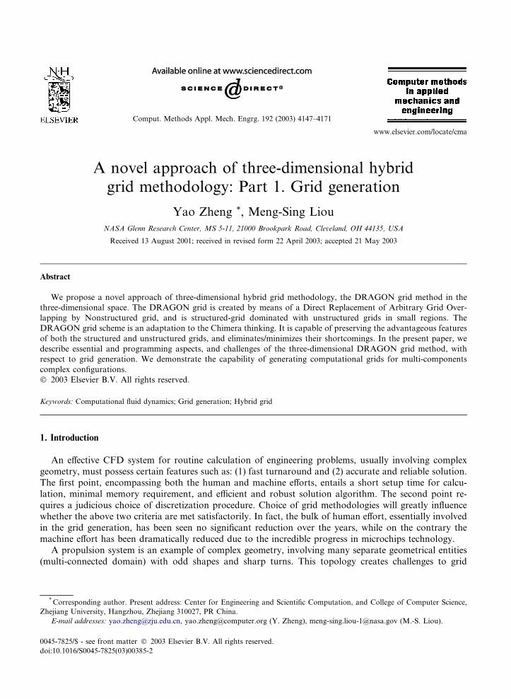
Fig. 5. Interface between structured and nonstructured grids in a three-dimensional DRAGON grid.


Fig. 5. This restriction may arise from the grid generation procedure or the requirement to adapt to the

physical phenomena. In Fig. 5, Points 1, 2, 3, 4, 5 and 6 on the structured grid are made coincident with the

corresponding ones on the unstructured grid. Therefore, a scheme can be easily developed to meet flux

conservation at common faces without resorting to interpolation of fluxes.

Occasionally, there might be areas of different grid spacings in an interfacial region between the struc-

tured and unstructured grids, as shown in Fig. 4(b). This is due to the requirements in the grid generation

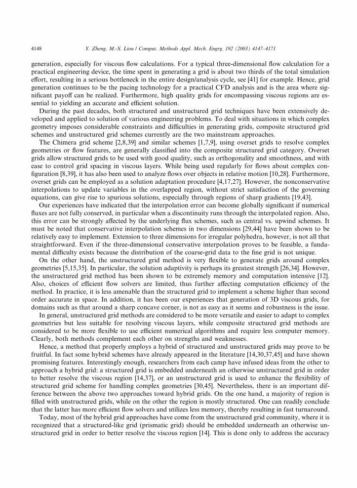
stage, and/or those to reflect the associated physical phenomena.As an example, Figs. 6 and 7 depict a DRAGON grid for the compressor drum cavity problem. This grid

is created from a base structured grid, where there are both overlapped domains and voids. The structured

grid is body-fitted, and of high quality for viscous flow simulation. The easily generated unstructured grid

Fig. 6. DRAGON grid for the compressor drum cavity problem. The outer rim barely reveals the third dimension.

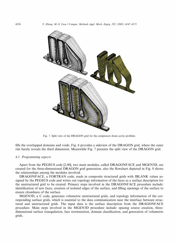
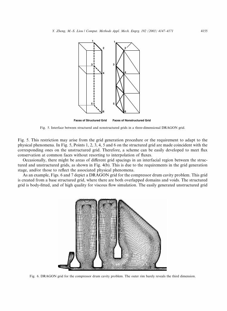
Fig. 7. Split view of the DRAGON grid for the compressor drum cavity problem.


fills the overlapped domains and voids. Fig. 6 provides a sideview of the DRAGON grid, where the outer

rim barely reveals the third dimension. Meanwhile Fig. 7 presents the split view of the DRAGON grid.

4.1. Programming aspects

Apart from the PEGSUS code [2,40], two main modules, called DRAGONFACE and MGEN3D, arecreated for the three-dimensional DRAGON grid generation, also the flowchart depicted in Fig. 8 shows

the relationships among the modules involved.

DRAGONFACE, a FORTRAN code, reads in composite structured grids with IBLANK values as-

signed by the PEGSUS code and writes out topology information of the faces as a surface description for

the unstructured grid to be created. Primary steps involved in the DRAGONFACE procedure include:

identification of new faces, creation of isolated edges of the surface, and filling openings of the surface to

ensure closedness of the surface.

MGEN3D, a C code, generates volumetric unstructured grids, and topology information of the cor-responding surface grids, which is essential to the data communication near the interface between struc-

tured and unstructured grids. The input data is the surface description from the DRAGONFACE

procedure. Main steps involved in the MGEN3D procedure include: spacing source creation, three-

dimensional surface triangulation, face reorientation, domain classification, and generation of volumetric

grids.

Composite Structured Grids

Domain Connectivity (PEGSUS)

Unstructured Grid Generation (MGEN3D)Surface and Volume Grids

Faces for Unstructured Grids (DRAGONFACE)

DRAGON Grid

Fig. 8. Program modules involved in the three-dimensional DRAGON grid generation.


4.2. Surface generation for nonstructured grids

4.2.1. Basics of resurfacing module

In the DRAGON gridding procedure, a void domain between structured grids is to be filled with anunstructured grid. Meanwhile a domain occupied by overlapped structured grids is also to be replaced with

an unstructured grid. Before the filling and replacement, quadrilateral (and then triangular) surface ele-

ments are constructed to describe the boundary of the volume, where a great deal of element/element

classification for the volumetric structured grids is involved. DRAGONFACE, a resurfacing module, has

been developed for this purpose, in conjunction with employing the existing PEGSUS code, which cuts the

overlapped regions and provides the associated blanking information.

A surface element consists of several edges. An edge is referred to as an isolated edge, if it belongs to only

one element of the surface. For a general surface, there are many edges, which belong to two neighboringelements, and clearly these edges are not isolated edges. Furthermore, for a closed surface, there are no

isolated edges; for an open surface, the corresponding isolated edges are bounding the openings of the

surface. Therefore, in order to close the surface, it is natural to establish the isolated edges first, and then to

identify facets which fill the openings.

In the following discussion, a special three-dimensional structured grid, namely 2.5-dimensional grid, is

to be mentioned. A 2.5-dimensional grid is a two-dimensional grid, except for being topologically trans-

formed (such as swept, rotated, and swept/rotated). Although the corresponding geometry is in three di-

mensions, it can be obtained by means of extrusion from a two-dimensional geometry, and the grid can bebuilt based on a two-dimensional base grid via extrusion.

Referring to Fig. 9, a flow chart of the DRAGONFACE module, we list the primary steps as follows:

(1) Read in composite structured grids and the associated IBLANK values assigned by the PEGSUS code.

(2) Identify new faces based on connectivity information of the volumetric grid elements, taking into ac-

count the known IBLANK values.

(3) Assign coordinates and set flags for the points associated with the newly defined faces. Update

IBLANK values if necessary to ensure that a closed surface is available.(4) Calculate default tolerance for determining coincident points.

(5) Flag edge entries based on the surface information. With the help of a sorting scheme, establish isolated

edges.

Read in Structured Gridswith IBLANK Values

Identify New Faces

Assign Coordinates and Set Point Flags

Check Closedness of the Surface

Calculate Default Geometry Tolerance

Flag Edge Entries

Identify Openings for General Cases(addwal3)

2.5-Dimensional?

No

Fill Gaps in the J and K Directions(addwal1)

Yes

Identify Openings in the L Planes(addwal3)

Fill Gaps or Identify Openings

Fig. 9. Flow chart of the DRAGONFACE procedure.


(6) If the grid is 2.5-dimensional in the sense of topology, and the L direction is assumed to be the one

which the third dimension lies in without loss of generality, then perform Operations addwal1 and add-wal2. Otherwise perform Operation addwal3 for general cases. In summary, we can list:addwal1: Fill gaps in the J and K directions;

addwal2: Identify openings in the L planes; and

addwal3: Identify openings for general cases.

4.2.2. Defining closed surfaces

Here we will dissect schemes of filling gaps and identifying openings in the DRAGONFACE procedure

(refer to Fig. 9), which are the master part of the procedure. Operation addwal1 is designed to fill gaps in the

J and K directions for 2.5-dimensional cases, and Fig. 10 illustrates this operation for the configurationinvolved in a turbine branch-duct problem. The detailed steps of this operation are itemized as follows:

(1) Establish segments along the isolated edges of the faces defined so far.

(2) Identify turning points on the segments. A point is referred to as a turning point if there exist two seg-

ments through the point, where one segment is on a J–K plane, but the other is not. Refer to Fig. 11,

Points A, B, C, and D are turning points.

(3) If Points A and B, and points C and D are pairs of coincident points, then zip the seam denoted by

segments AC and BD.

Fig. 10. Gap filling operation working on the surface description for a turbine branch-duct problem. The gaps filled are marked by

circles.

Fig. 11. Illustration of filling a gap in the J and K directions and definition of turning points.


(4) If Points A and B, and Points C and D are not pairs of coincident points, then fill the gap ABDC with

quadrilaterals, referring to Fig. 11.


Operation addwal2 is designed to identify openings in the L planes for the 2.5-dimensional case and thesteps involved are given as follows:


(2) Identify turning points on the segments if they exist.

(3) Based on the segments, identify openings in the L planes. This will result in a set of closed loops of seg-

ments (refer to Fig. 12).

(4) Determine an approximate fitting plane for the loops to be projected to.

(5) According to the projection, determine location relationship of the loops (insidedness) by means of areamethod, rebuild loops if necessary and then create the surface description. For the example shown in

Fig. 12, the corresponding surface region is a region (i.e., an opening to be filled) with two isolated is-

lands inside it, where loops L2 and L3 are considered to be inside loop L1. These loops together define a

surface region, a shaded area in Fig. 12.

Fig. 13 shows a surface definition for unstructured grid generation for a turbine branch-duct problem.

This definition is the result from the DRAGONFACE procedure before the addwal2 operation has been

performed. The corresponding faces have not yet been split into triangles, and are still in the quadrilateralform. Fig. 14 depicts unstructured grids generated to fill the gap regions between structured grids.

For general cases, Operation addwal3 has been designed to identify openings towards establishing the

surface definition. The corresponding steps involved are as below:


(2) Construct a set of segment loops from the segments created above.

(3) Determine an approximate fitting plane for the loops to be projected to.

(4) According to the projection, determine location relationship of the loops (insidedness) by means of areamethod, rebuild loops if necessary, and then create the surface description.

Fig. 12. Illustration of identifying an opening in the L planes.

Fig. 13. Surface description for unstructured grid generation for the turbine branch-duct problem.

Fig. 14. Unstructured grids created based on the surface description shown in Fig. 13.



4.3. Generation of nonstructured grids

4.3.1. Basics of the generation method

The generation of nonstructured grids is essential to the three-dimensional DRAGON gridding. The

specific task is the implementation of a tetrahedral grid generation kernel. This kernel is the key to the

success of DRAGON gridding, and serves as an engine to create tetrahedral grids for particular domains.

Currently there are two basic types of tetrahedral grid generation schemes: advancing front approach [33]

and Delaunay triangulation [20]. Also a coupled approach [11] has been proposed to take the advantages ofboth schemes. After an investigation into these schemes, Delaunay triangulation has been chosen, partly

taking into account the time frame required in the development.

The algorithm of the MGEN3D code evolves from the framework of previous work [20,46,47], and is a

Delaunay-type method. The Steiner point [31] creation algorithm has been incorporated into this grid

generator. Surface grids are created based on two-dimensional geometries by means of coordinate mapping.

Volume grids are generated through three-dimensional triangulation and interior point creation based on

the surface grids. Boundary surface conformity is gained via edge swapping, boundary edge and surface

recovery. In order to control the quality of the resulting grids, several parameters have been introduced,such as the baseline grid spacing and the grid regularity parameter.

Algorithms involved in the MGEN3D procedure are summarized as follows:

(1) Surface description generated via the DRAGONFACE procedure is read in, while spacing source cre-

ation is performed automatically (refer to Section 4.3.2 below).

(2) Surface triangulation is carried out taking into account the baseline grid spacing, point and line source

distribution.

(3) From this surface triangulation, the face orientation may not be consistent over the whole surface. Facereorientation is necessary and essential, which ensures that all the normals of the triangular faces are

consistently outwards or inwards.

(4) Domain classification is performed to provide domain information of the geometry specified by the

above surface definition.

(5) Volumetric grids are generated for the domains one by one until the end. Data of the assembly of in-

dividual volumetric grids, including nodal coordinates and connectivities, are finally created.

4.3.2. Automatic spacing source creation

A conversion from the quadrilateral grid-based surface into the triangular grid-based surface is neces-

sary, in order to generate tetrahedral grids. From time to time, there might be sharp changes in the sizes of

the quadrilaterals. In order to obtain a surface grid, and then a volume grid, with smooth variation of point

spacing, certain controls need to be introduced. Sometimes certain quadrilaterals are stretched too much,

then another type of control may be employed, in order to get a grid with limited stretch ratio of its ele-

ments.

A point source is assigned with two radii and a spacing value. Within the first radius the elements will be

generated which have a length scale that is similar to the spacing value specified. The element length scalethen exponentially increases to a global spacing value outside the first radius. The incremental rate of

expansion of point spacing is defined by the relationship shown in Fig. 15. This expression prescribes the

spacing at the outer radius to be twice that at the inner radius. Fig. 15 illustrates the influence of a point

source on the point spacing variation. In light of the concept of point source, the concept of line source can

be introduced. A line source has a cylindrical range of influence. The point and line source distribution

control surface grid generation, and further volumetric grid generation as well.

The procedure to create point and line sources to control the spacing of the new surface grids has been

automated during the DRAGONFACE process. Fig. 16 depicts point sources, which reflect the spacing

Fig. 15. Illustration of the influence of a point grid source on the point spacing variation.

Fig. 16. Illustration of automatic spacing source creation during unstructured grid generation: (a) surface description; (b) point

sources created to reflect the spacing variation of the structured grid; (c) line sources introduced in the area of stretched elements;

(d) volumetric grid; and (e) volumetric grid with a part cut.


variation of the structured grid, and line sources, which are introduced in the neighborhoods of stretchedelements. A coloring scheme is used to display the intensity variations of various sources.


A baseline grid spacing can take a value, which is of the same order as the average grid size of thequadrilaterals. Then roughly a quadrilateral, with an edge length larger than the baseline grid spacing, will

be divided into more than two triangles. This baseline grid spacing value is only a reference value for the

grid generation. And the point and line sources provide a further and local control on the overall grid

spacing variation.

If the maximal edge length of a quadrilateral is larger than a given grid spacing threshold, then a point

source will be created to influence the neighborhood of the quadrilateral. If the stretch ratio of a quadri-

lateral is larger than a given stretch threshold, then a line source will be generated with an influence on the

neighborhood of the quadrilateral.

4.4. Special treatment for viscous grids

By examining Figs. 13 and 14, we find that the unstructured grids are much finer than the structured

grids nearby. The small grid spacing is due to the fact that the spacing of the structured grids vary in the

spanwise direction, with the smallest spacing values at the top and bottom of the geometries in that di-

rection to account for the viscous effects near the side walls (refer to Fig. 13). When an original quadri-

lateral element is greatly stretched, a line source will be automatically created within the framework of thestandard Delaunay-type gridding algorithm, which usually tends to yield a finer grid locally. The standard

Delaunay-type grid generation normally leads to isotropic grids. If an extension to the standard method

were made, in order to create stretched grids, then the unstructured grid shown in Fig. 14 could be coarser,

and some memory would be saved.

As an alternative, special treatment could be conducted by means of leaving out the regions within

viscous layers during the first phase of unstructured grid generation. Then we could grow viscous layers in a

Fig. 17. Unstructured grid domains for the turbine branch-duct problem, after the first phase of unstructured grid generation.

Fig. 18. Unstructured grid domains considering viscous layers for the turbine branch-duct problem.


form of structured-grid-like tetrahedral elements, taking into account the surface grids of the tetrahedral

grids previously created. The operation of growing viscous layers is quite straightforward, where base

surface elements, their normals, and layer thicknesses are the only information required. Fig. 17 shows the

unstructured grid domains leaving out viscous layers, based on the surface description given in Fig. 13. And

finally the whole unstructured grid domains of the DRAGON grid for the turbine branch-duct problem are

depicted in Fig. 18, after the operation of growing viscous layers.

5. Industrial examples

Three examples often seen in propulsion systems have been introduced to validate the three-dimensional

DRAGON gridding methodology. These include a compressor drum cavity, turbine branch-duct––a

portion of an internal coolant passage, and a film-cooled turbine vane. We have seen in Figs. 6 and 7 the

three-dimensional DRAGON grid for the compressor drum cavity.Fig. 19 is a schematic of the turbine branch-duct. It shows rows of pins placed in a turbine coolant

passage used to promote mixing. During the creation of Chimera and/or DRAGON grids, once a cylin-

drical structured grid is generated for a pin, a duplication of it can be added and moved to any place to

assess their effects on aerodynamic performance and heat transfer. For the generation of the overlaid

structured grids, it is just as easy to add/delete components to/from the configuration. This flexibility clearly

has great potential for design purposes. Fig. 20 followed by Fig. 21 shows the DRAGON grid for the

computational problem.

Fig. 20. DRAGON grid for the turbine branch-duct problem.

Fig. 21. Close-up view of the DRAGON grid for the turbine branch-duct problem.

Fig. 19. Schematic of the turbine branch-duct.


Lastly, we consider a typical film-cooled turbine vane, whose schematic is shown in Fig. 22. This ge-ometry includes the vane, coolant plena, and 33 holes inside of the vane. Fig. 23 depicts the whole resulted

Fig. 23. DRAGON grid for the film-cooled turbine vane problem.

Fig. 22. Schematic of the vane cross-section and coolant holes.


DRAGON grid, where the connecting regions between the 33 holes and the flow domain are filled withunstructured grids. Fig. 24 is a close-up view of this DRAGON grid in the leading edge region of the

Fig. 24. Close-up view of the DRAGON grid in the leading edge region of the film-cooled turbine vane.


film-cooled turbine vane. Furthermore, Fig. 25 provides a deep insight into this DRAGON grid by means

of cutting through the grid, where attention has only been paid to the leading edge region.

During the DRAGON grid generation, the 33 individual structured grids for the holes have been created

without trying to topologically join them to the grids representing the external flow domain, which wouldbe required in the multiblock grid generation [13]. From this point of view, the DRAGON grid scheme

could be considered as a more flexible and easier approach.

Fig. 25. Cut-through view of the DRAGON grid in the leading edge region of the film-cooled turbine vane, showing the internal plena

and coolant holes inside the vane.


However, the user may prefer to have structured grids presented in a specific region, due to the physicaland numerical characteristic. For instance in this example, the user might like to use structured grids to fill

the connecting regions between the holes and the flow domain. Because the DRAGON grid is actually

created by using a base composite structured grid, one can make structured grids presented in a particular

region, as long as the base composite structured grid is generated with such an intention.

6. Concluding remarks

In the present work, we have presented the essentials and challenges of a new three-dimensional hybrid

grid, termed DRAGON grid, methodology. This methodology attempts to blend the advantageous features

of both the structured and unstructured grids, while eliminating or minimizing their respective short-

comings. As a result, the method is very amenable to quickly creating quality viscous grids for various

individual components with complex shapes found in an engineering system. The base composite structured

grid does not need to cover the whole domain. This makes the corresponding structured grid generation

much easier. We concluded that the applications of three-dimensional DRAGON grid technology are very

encouraging because the objectives of quickly generating quality grids for complex geometries have beendemonstrated.

Computationally, the resulting grid drastically reduces the memory required in the unstructured grid and

makes more efficient solvers accessible because the major portion of the DRAGON grid is in the form of

the structured grid. Moreover, high quality viscous grids are inherited in the process, unlike in the un-

structured grid generation, where structured-grid-like grids (such as prismatic layers) can be added, but are

still based on the unstructured-grid data structure.

Acknowledgements

We thank James D. Heidmann for kindly providing us the geometry of the film-cooled turbine vane, and

Kumud Ajmani for generating the Chimera grids for the compressor drum cavity and the turbine branch-

duct. We also thank Pieter G. Buning for providing us the picture of the Chimera grid for the integrated

space shuttle geometry.

References

[1] E.H. Atta, Component-adaptive grid interfacing, AIAA Paper 81-0382, AIAA 19th Aerospace Sciences Meeting, St. Louis, MO,

1981.

[2] J.A. Benek, J.L. Steger, F.C. Dougherty, P.G. Buning, Chimera: A grid-embedding technique, Report AEDC-TR-85-64, Arnold

Engineering Development Center, April 1986.

[3] M.J. Berger, On conservation at grid interfaces, NASA ICASE Report 84-43, Institute for Computer Applications in Science and

Engineering, NASA Langley Research Center, Hampton, VA, September 1984.

[4] M.J. Berger, J. Oliger, Adaptive mesh refinements for hyperbolic partial differential equations, J. Comput. Phys. 53 (1984) 484–

512.

[5] K.R. Blake, G.S. Spragle, Unstructured 3D Delaunay mesh generation applied to planes, trains and automobiles, AIAA Paper 93-

0673, AIAA 31th Aerospace Sciences Meeting & Exhibit, Reno, NV, January 1993.

[6] A. Bowyer, Computing Dirichlet tessellations, Comput. J. 24 (2) (1981) 162–166.

[7] D.L. Brown, G. Chesshire, W.D. Henshaw, Getting started with CMPGRD, Introductory User�s Guide and Reference Manual,

LA-UR-89-1294, Los Alamos National Laboratory, 1989.

[8] P.G. Buning, I.T. Chiu, F.W. Martin Jr., R.L. Meakin, S. Obayashi, Y.M. Rizk, J.L. Steger, M. Yarrow, Flowfield simulation of

the space shuttle vehicle in ascent, in: Proc. the Fourth International Conference on Supercomputing, Santa Clara, CA, April

1989, pp. 20–28.


[9] G. Chesshire, W.D. Henshaw, Composite overlapping meshes for the solution of partial differential equations, J. Comput. Phys.

90 (1990) 1–64.

[10] F.C. Dougherty, J.A. Benek, J.L. Steger, On application of Chimera grid schemes to store separation, NASA TM 88193, NASA,

October 1985.

[11] P.J. Frey, H. Borouchaki, P.-L. George, 3D Delaunay mesh generation coupled with an advancing-front approach, Comput.

Methods Appl. Mech. Engrg. 157 (1998) 115–131.

[12] F. Ghaffari, On the vortical-flow prediction capability of an unstructured-grid Euler solver, AIAA Paper 94-0163, AIAA 32nd

Aerospace Sciences Meeting & Exhibit, Reno, NV, January 1994.

[13] J.D. Heidmann, D. Rigby, A.A. Ameri, A three-dimensional coupled internal/external simulation of a film-cooled turbine vane,

Trans. ASME, J. Turbomach. 122 (2000) 348–359.

[14] D.G. Holmes, S.D. Connell, Solution of the 2D Navier–Stokes equations on unstructured adaptive grids, AIAA Paper 89-1932,

AIAA 9th CFD Conference, Buffalo, NY, June 1989.

[15] A. Jameson, T.J. Baker, N.P. Weatherill, Calculation of inviscid transonic flow over a complete aircraft, AIAA Paper 86-0103,

AIAA 24th Aerospace Sciences Meeting, Reno, NV, January 1986.

[16] K.-H. Kao, M.-S. Liou, Advance in overset grid schemes: From Chimera to DRAGON grids, AIAA J. 33 (10) (1995) 1809–1815.

[17] K.-H. Kao, M.-S. Liou, C.Y. Chow, Grid adaptation using Chimera composite overlapping meshes, AIAA J. 32 (5) (1994) 942–

949.

[18] G.H. Klopfer, G.A. Molvik, Conservative multi-zonal interface algorithm for the 3D Navier–Stokes equations, AIAA Paper 91-

1601-CP, AIAA 10th CFD Conference, Honolulu, Hawaii, June 1991.

[19] A. Lerat, Z.N. Wu, Stable conservative multidomain treatments for implicit Euler solvers, J. Comput. Phys. 123 (1996) 45–64.

[20] R.W. Lewis, Y. Zheng, D.T. Gethin, Three-dimensional unstructured mesh generation: Part 3. Volume meshes, Comput. Methods

Appl. Mech. Engrg. 134 (3/4) (1996) 285–310.

[21] M.-S. Liou, K.-H. Kao, in: D.A. Caughey, M.M. Hafez (Eds.), Progress in grid generation: From Chimera to DRAGON grids,

NASA TM 106709, Lewis Research Center, Cleveland, OH, August 1994; Also, in: D.A. Caughey, M.M. Hafez (Eds.), Frontiers

of Computational Fluid Dynamics, John Wiley & Sons, 1994 (chapter 21).

[22] M.-S. Liou, Y. Zheng, Development of 3D DRAGON grid method for complex geometry, in: D.A. Caughey, M.M. Hafez (Eds.),

Frontiers of Computational Fluid Dynamics––2002, World Scientific Publishing Company, Singapore, 2001, pp. 299–317.

[23] M.-S. Liou, Y. Zheng, A three-dimensional hybrid grid: DRAGON grid, in: N. Satofuka (Ed.), Computational Fluid Dynamics

2000, Proceedings of the First International Conference on Computational Fluid Dynamics (1st ICCFD), Kyoto, Japan, July,

2000, Springer-Verlag, Berlin, 2001, pp. 113–118.

[24] M.-S. Liou, Y. Zheng, A flow solver for three-dimensional dragon grids, NASA TM 2002-211512, NASA, May 2002.

[25] M.-S. Liou, Y. Zheng, A novel approach of three-dimensional hybrid grid methodology: Part 2. Flow solution, Comput. Methods

Appl. Mech. Engrg. 192 (35–36) (2003), next article in this issue.

[26] R. L€oohner, An adaptive finite element scheme for transient problems in CFD, Comput. Methods Appl. Mech. Engrg. 61 (3) (1987)

323–338.

[27] R.L. Meakin. On adaptive refinement and overset structured grids, AIAA Paper 97-1858, AIAA 13th CFD Conference,

Snowmass, CO, June 1997.

[28] R.L. Meakin, N. Suhs, Unsteady aerodynamic simulation of multiple bodies in relative motion, AIAA Paper 89-1996-CP, AIAA

9th CFD Conference, Buffalo, NY, June 1989.

[29] Y.J. Moon, M.-S. Liou, Conservative treatment of boundary interfaces for overlaid grids and multi-level grid adaptations, AIAA

Paper 89-1980-CP, AIAA 9th CFD Conference, Buffalo, NY, June 1989.

[30] K. Nakahashi, S. Obayashi, FDM-FEM zonal approach for viscous flow computations over multiple-bodies, AIAA Paper 87-

0604, AIAA 25th Aerospace Sciences Meeting, Reno, NV, January 1987.

[31] A. Okabe, B. Boots, K. Sugihara, Spatial Tessellations: Concepts and Applications of Voronoi Diagrams, John Wiley & Sons,

Chichester, 1992.

[32] D.G. Pearce, S.A. Stanley, F.W. Martin Jr., R.J. Gomez, G.J. Le Beau, P.G. Buning, W.M. Chan, I.T. Chiu, A. Wulf, V. Akdag,

Development of a large scale Chimera grid system for the space shuttle launch vehicle, AIAA Paper 93-0533, AIAA 31st

Aerospace Sciences Meeting, Reno, NV, January 1993.

[33] J. Peraire, J. Peiro, K. Morgan, Adaptive remeshing for three-dimensional compressible flow computations, J. Comput. Phys. 103

(1992) 269–285.

[34] J. Peraire, M. Vahdati, K. Morgan, O.C. Zienkiewicz, Adaptive remeshing for compressible flow computations, J. Comput. Phys.

72 (1987) 449–466.

[35] M. Posenau, Unstructured Grid Generation Techniques and Software, NASA CP-10119 NASA, 1993.

[36] M.M. Rai, A conservative treatment of zonal boundaries for Euler equation calculations, J. Comput. Phys. 62 (1986) 472–503.

[37] M. Soetrisno, S.T. Imlay, D.W. Roberts, A zonal implicit procedure for hybrid structured-unstructured grids, AIAA Paper 94-

0645, AIAA 32nd Aerospace Sciences Meeting & Exhibit, Reno, NV, 1994.


[38] J.L. Steger, Thoughts on the Chimera method of simulation of three-dimensional viscous flow, in: M.-S. Liou, L.A. Povinelli

(Eds.), Proc. Computational Fluid dynamics Symposium on Aeropropulsion, NASA CP-3078, 1990, pp. 1–10.

[39] J.L. Steger, J.A. Benek, On the use of composite grid schemes in computational aerodynamics, Comput. Methods Appl. Mech.

Engrg. 64 (1/3) (1987) 301–320.

[40] N.E. Suhs, R.W, Tramel, PEGSUS 4.0 User�s Manual, AEDC-TR-91-8, Calspan Corporation/AEDC Operations, Arnold AFB,

TN, November 1991.

[41] R. Taghavi, Automatic, parallel and fault tolerant mesh generation from CAD on Cray Research supercomputers, Technical

Report, Cray User Group Conference, Tours, France, 1994.

[42] J.L. Thomas, R.W. Walters, T. Reu, F. Ghaffari, R. Weston, J.M. Luckring. Patched-grid algorithm for complex configurations

directed towards the F/A-18 aircraft, AIAA Paper 89-0121, AIAA 27th Aerospace Sciences Meeting, Reno, NV, January 1989.

[43] Z.J. Wang, N. Hariharan, R. Chen, Recent developments on the conservation property of Chimera, AIAA Paper 98-0216, AIAA

36th Aerospace Sciences Meeting & Exhibit, Reno, NV, January 1998.

[44] Z.J. Wang, H.Q. Yang, A unified conservative zonal interface treatment for arbitrarily patched and overlapped grids, AIAA Paper

94-0320, AIAA 32nd Aerospace Sciences Meeting & Exhibit, Reno, NV, January 1994.

[45] N.P. Weatherill, On the combination of structured-unstructured meshes, in: S. Sengupta, J. H€aauser, P.R. Eiseman, J.F. Thompson

(Eds.), Numerical Grid Generation in Computational Fluid Mechanics, Pineridge Press, Swansea, UK, 1988, pp. 729–739.

[46] Y. Zheng, R.W. Lewis, D.T. Gethin, Three-dimensional unstructured mesh generation: Part 1. Fundamental aspects of

triangulation and point creation, Comput. Methods Appl. Mech. Engrg. 134 (3/4) (1996) 249–268.

[47] Y. Zheng, R.W. Lewis, D.T. Gethin, Three-dimensional unstructured mesh generation: Part 2. Surface meshes, Comput. Methods

Appl. Mech. Engrg. 134 (3/4) (1996) 269–284.

[48] Y. Zheng, M.-S. Liou, Progress in the three-dimensional DRAGON grid scheme, AIAA Paper 2001-2540, Presented at the 15th

AIAA Computational Fluid Dynamics Conference, CA, USA, June, 2001.

[49] Y. Zheng, M.-S. Liou, K.C. Civinskas, Development of three-dimensional DRAGON grid technology, NASA TM 1999-209458,

NASA, November 1999.

a novel approach of three-dimensional hybrid grid ... · a novel approach of three-dimensional...

Documents