remote sensing

Article

A Novel Approach for the Determination of theHeight of the Tropopause from Ground-BasedGNSS Observations

Jorge Mendez Astudillo 1, Lawrence Lau 2,* , Yu-Ting Tang 3 and Terry Moore 4

1 International Doctoral Innovation Center, University of Nottingham Ningbo China, Ningbo 315100, China;Jorge.mendez@nottingham.edu.cn

2 Department of Civil Engineering, University of Nottingham Ningbo China, Ningbo 315100, China3 School of Geographical Sciences, University of Nottingham Ningbo China, Ningbo 315100, China;

Yuting.tang@nottingham.edu.cn4 Nottingham Geospatial Institute, the University of Nottingham, Nottingham NG7 2RD, UK;

Terry.Moore@nottingham.ac.uk* Correspondence: Lawrence.Lau@nottingham.edu.cn; Tel.: +86-574-8818-9032

Received: 24 November 2019; Accepted: 12 January 2020; Published: 16 January 2020�����������������

Abstract: In this paper, we present a new method to calculate the height of the second lapse-ratetropopause (LRT2) using GNSS high-precision data. The use of GNSS data for monitoring theatmosphere is possible because as the radio signals propagate through the troposphere, they aredelayed according to the refractive index of the path of the signal. We show that by integrating thevertical profile of the refractive index in the troposphere, we are able to determine the altitude ofLTR2. Furthermore, as GNSS data is available from many stations around all latitudes of the globeand make up a network with high spatial and temporal resolution, we can monitor the diurnal cycleof the variables related to the refractive index of the path of the signal. A comparison between theheights of the LRT2 obtained with radiosonde data and with this novel method is presented in thepaper, and it shows good agreement. The average difference found is ≤1 km for stations between thelatitudes of 30◦S and 30◦N.

Keywords: Lapse Rate Troposphere (LRT); Zenith Tropospheric Delay (ZTD); GNSS atmosphericmonitoring

1. Introduction

Accurate weather data is required to correctly assess weather issues and to produce accuratemodels that help mitigate climate issues such as global warming. One atmospheric parameter that isimportant to monitor is the height of the tropopause. The tropopause is defined by the second and firstlapse-rate tropopauses (LRT2 and LRT1, respectively). Changes in the height of the global tropopausecan be an indicator of anthropogenic climate change [1–3]. Also, it is relevant to study the tropopauselayer because it separates the troposphere and stratosphere, which have different characteristics withrespect to chemical composition and static stability, which affect the tropopause layer [4]. Furthermore,the tropopause region plays an important role in the stratosphere–troposphere exchange [5].

The troposphere is the layer of the atmosphere closest to the earth’s surface which extends toabout 18 km above sea level. Between the troposphere and the stratosphere, there is a middle layercalled the tropopause [6]. This layer starts with the LRT1 and ends at the LRT2 [7]. The next layeris called the stratosphere. Figure 1 illustrates the approximate height of each layer, as well as thetemperature profile through the layers.

Remote Sens. 2020, 12, 293; doi:10.3390/rs12020293 www.mdpi.com/journal/remotesensing

Remote Sens. 2020, 12, 293 2 of 18

Remote Sens. 2020, 12, x FOR PEER REVIEW 2 of 18

Figure 1. Location of the tropopause and the troposphere and the profile of temperature in the troposphere.

The LRT1 can be defined in terms of the gradient of temperature against altitude. For example, Seidel and Randel [8], based on the World Meteorological Organization (WMO), defined the LRT1 as being at the altitude where the lapse rate of the temperature decreases to −2 °C/km, provided that within 2 km above this point, the average lapse rate does not exceed 2 °C/km. The LRT2 is defined as the point above the first tropopause, 1 km beyond which the average lapse exceeds 3 °C/km; any point higher than this 1-km layer, the lapse exceeds 3 °C/km.

In the profile of temperature showed in Rieckh et al. [9], as the altitude increases to 10 km, the temperature decreases up to 200 K (−73 °C). Then, there is an inflection point where the temperature remains almost constant as the altitude further increases; this point is defined as LRT1. It has been found that in the northern hemisphere between latitudes 20° and 40°, the height of the LRT1 is approximately 15 km above sea level [9]. According to the results obtained by Feng et al. [6], the LRT2 can be found at altitudes of around 14 and 25 km, depending on the latitude where the measurement is done. The tropopause layer is, therefore, defined as the distance between LRT2 and LRT1. The tropical tropopause is defined as being between the latitudes of 30°N and 30°S.

There are three main methods to obtain the height of the tropopause: the use of radiosonde data [4,6,8,10], the use of GPS Radio occultation (GPS-RO) [9], and the use of Very High Frequency (VHF) radars [11]. Radiosonde is the data source most commonly used. Other sources that have been used to study the tropopause are Atmospheric Infrared Sounder (AIRS) [12], Infrared Atmospheric Sounding Interferometer (IASI) [13], and the High-Resolution Infrared Radiation Sounder (HIRS).

Radiosonde data is readily available from stations around the globe; they provide environmental measurements such as temperature, humidity, pressure, etc. at different heights in one sounding. Radiosondes take measurements for the whole troposphere up to the geopotential height where the pressure is 100 hPa; however, radiosondes have a poor temporal resolution, because the measurements are only taken every 12 h. Its vertical resolution of 2 km requires the use of complex mathematical models to interpolate the temperature transition to determine the height of the tropopauses. In addition, the unique temperature profile along the altitude also increases the complexity of the mathematical models required to process the radiosonde data [8]. Because of a few potential inflection points in the temperature changes along the altitude, the mathematical model needs to describe a curve, rather than a linear relationship. The spatial resolution of the stations remains poor, even though developed algorithms are used to increase it.

The GPS-RO method provides near-vertical profiles of atmospheric thermodynamic variables with high vertical resolution (better than 1 km) and global coverage [9]. Using AIRS data, an error of approximately 4 K is found for temperatures around the tropopause [12]. In a study by Lerner et al. [13], the authors used IASI data and found that in the troposphere (i.e., below 200 hPa), the retrieved profiles exhibited temperature errors of less than 1 K and specific humidity errors of minus 10% at most heights, associated with a vertical resolution of 1.5–2 km. HIRS data provides a vertical resolution of 3–5 km in the troposphere.

Figure 1. Location of the tropopause and the troposphere and the profile of temperature inthe troposphere.

The LRT1 can be defined in terms of the gradient of temperature against altitude. For example,Seidel and Randel [8], based on the World Meteorological Organization (WMO), defined the LRT1 asbeing at the altitude where the lapse rate of the temperature decreases to −2 ◦C/km, provided thatwithin 2 km above this point, the average lapse rate does not exceed 2 ◦C/km. The LRT2 is defined asthe point above the first tropopause, 1 km beyond which the average lapse exceeds 3 ◦C/km; any pointhigher than this 1-km layer, the lapse exceeds 3 ◦C/km.

In the profile of temperature showed in Rieckh et al. [9], as the altitude increases to 10 km, thetemperature decreases up to 200 K (−73 ◦C). Then, there is an inflection point where the temperatureremains almost constant as the altitude further increases; this point is defined as LRT1. It has beenfound that in the northern hemisphere between latitudes 20◦ and 40◦, the height of the LRT1 isapproximately 15 km above sea level [9]. According to the results obtained by Feng et al. [6], the LRT2can be found at altitudes of around 14 and 25 km, depending on the latitude where the measurement isdone. The tropopause layer is, therefore, defined as the distance between LRT2 and LRT1. The tropicaltropopause is defined as being between the latitudes of 30◦N and 30◦S.

There are three main methods to obtain the height of the tropopause: the use of radiosondedata [4,6,8,10], the use of GPS Radio occultation (GPS-RO) [9], and the use of Very High Frequency(VHF) radars [11]. Radiosonde is the data source most commonly used. Other sources that have beenused to study the tropopause are Atmospheric Infrared Sounder (AIRS) [12], Infrared AtmosphericSounding Interferometer (IASI) [13], and the High-Resolution Infrared Radiation Sounder (HIRS).

Radiosonde data is readily available from stations around the globe; they provide environmentalmeasurements such as temperature, humidity, pressure, etc. at different heights in one sounding.Radiosondes take measurements for the whole troposphere up to the geopotential height where thepressure is 100 hPa; however, radiosondes have a poor temporal resolution, because the measurementsare only taken every 12 h. Its vertical resolution of 2 km requires the use of complex mathematicalmodels to interpolate the temperature transition to determine the height of the tropopauses. In addition,the unique temperature profile along the altitude also increases the complexity of the mathematicalmodels required to process the radiosonde data [8]. Because of a few potential inflection points inthe temperature changes along the altitude, the mathematical model needs to describe a curve, ratherthan a linear relationship. The spatial resolution of the stations remains poor, even though developedalgorithms are used to increase it.

The GPS-RO method provides near-vertical profiles of atmospheric thermodynamic variableswith high vertical resolution (better than 1 km) and global coverage [9]. Using AIRS data, an errorof approximately 4 K is found for temperatures around the tropopause [12]. In a study by Lerner etal. [13], the authors used IASI data and found that in the troposphere (i.e., below 200 hPa), the retrievedprofiles exhibited temperature errors of less than 1 K and specific humidity errors of minus 10% at most

Remote Sens. 2020, 12, 293 3 of 18

heights, associated with a vertical resolution of 1.5–2 km. HIRS data provides a vertical resolution of3–5 km in the troposphere.

The numerical weather prediction (NWP) and climate monitoring communities require a retrievalaccuracy of less than 1 K in 1-km layers for temperature and better than 15% in 2-km layers forwater vapor in the troposphere [13]. Thus, in order to improve the spatial resolution of the estimatedthickness of the troposphere without increasing the complexity of mathematical models, an alternativemethod of measuring the height of the first and second lapse rate tropopauses is proposed based inGlobal Navigation Satellite System data (GNSS).In this paper, a new method is proposed to obtain afine spatial resolution of both LRT1 and LRT2 at different latitudes from GNSS data.

Global Navigation Satellite System (GNSS) has been widely used in positioning [14,15] andattitude determination [16,17]. Also, GNSS data has been used to monitor the atmosphere [18]. Theusage of GNSS signals for climate studies is gaining more interest as global warming becomes aserious challenge.

The method is novel because it uses of the Zenith Tropospheric Delay (ZTD), a by-product ofthe Precise Point Positioning (PPP) technique using Global Navigation Satellite System (GNSS) data.The ZTD can be used to determine the height of the troposphere because radio signals are delayeddepending on the radio refractive index of the travelling path. Thus, by mathematically modeling therefractivity profile of the troposphere, it is possible to solve for the path of the signal which correspondsto the troposphere thickness. The main advantage of using the ZTD is that the temporal resolution isincreased, as there is GNSS data every 30 s. Also, any GNSS receiver can be turned into a measuringstation which makes it possible to increase the spatial resolution. There are GNSS receivers embeddedin devices such as smartphones, car-navigation systems, etc. If the device supports carrier-phasetracking, the ZTD can be estimated from the PPP technique. The PPP positioning technique is widelyimplemented in many software and online services. A previous study [19] found that most onlinesoftware available for PPP obtained very close values for the estimation of the ZTD. Thus, we canexpect consistent results using any software.

The method presented in this paper makes it possible to estimate the height of the LRT1 with aprecision of 500 m from GNSS data once an adjustment parameter (derived with radiosonde data) isknown. In this study, only one year of data is used to test the method because in previous studies,such as the one by Mathew and Kumar [20], it was argued that once the height of the LRT had beencalculated, it could be applied globally to data from different years.

The paper is structured as follows. Section 2 describes the data used to measure the height ofthe LRT1 and LRT2, i.e., radiosonde data and GNSS data, and the new method proposed to measurethe height of the LRT1 from GNSS data is presented. Section 3 shows the results of the presentedtechnique. Section 4 comprises discussion of the results. Section 5 presents the conclusion drawn fromthis analysis.

2. Materials and Methods

2.1. Description of GNSS Data Sources

The International GNSS Service (IGS) operates 505 GNSS stations across the world. Differentproducts and observation data are provided by each station. Collectively, they provide data every dayin a year (some stations do not provide data daily). They are made publicly available through theirftp site (ftp://cddis.gsfc.nasa.gov/gnss). Observation data with a frequency of 30 s is available for allstations managed by the IGS. The IGS also provides navigation data and ephemeris used in the PPPtechnique. The latitudes, longitudes, and heights of 15 selected GNSS stations covering the latitudes of35◦N to 35◦S are given in Table 1 (values provided by the IGS). This data is used to determine LRT1and LRT2.

Remote Sens. 2020, 12, 293 4 of 18

Table 1. Details about IGS ZTD data used in this study. The code, latitude, longitude, and height areprovided by the IGS.

GNSS Stations

Code Lat (◦) Long (◦) Height (m) Location Country

JPLM 34.2 −118.17 423.99 Pasadena United StatesGMSD 30.56 131.02 142.65 Nakatane town JapanTWTF 24.95 121.16 203.12 Taoyuan TaiwanMKEA 19.8 −155.46 3754.7 Mauna Kea United StatesCNMR 15.23 145.74 64.4 Saipan United StatesDJIG 11.53 42.85 711.41 Djibouti Djibouti

KOUG 5.09 −52.64 107.25 Kourou French GuianaNAUR −0.55 166.93 46.3 Nauru, Yaren District NauruSEYG −4.68 55.53 −37.09 Pointe Larue SeychellesXMIS −10.45 105.69 261.58 Christmas Island Australia

ZAMB −15.46 28.31 1324.91 Lusaka ZambiaVACS −20.3 57.5 420.4 Vacoas MauritiusUFPR −25.45 −49.23 925.8 Curitiba Brazil

NNOR −31.05 116.19 234.98 New Norcia AustraliaSTR1 −35.31 149.01 800.03 Canberra Australia

2.2. Description of Radiosonde Data

The Integrated Global Radiosonde Archive (IGRA) run by the National Ocean and AtmosphereAdministration (NOAA) (https://www.ncdc.noaa.gov/data-access/weather-balloon/integrated-global-radiosonde-archive) contains radiosonde data from more than 2500 stations around the world. Moststations contain data from two soundings every day: one at 00:00 Coordinated Universal Time (UTC)and one at 12:00 UTC. For the validation of the values of LRT1 and LRT2 obtained with GNSS data, 15stations were chosen with the same latitude (because the height of the tropopause is highly associatedwith latitude) as the GNSS stations previously described. The latitude, longitude, and height of theradiosonde stations used in this study as reported by the IGRA are given in Table 2.

Table 2. Radiosondes selected for this study and their location.

Radiosonde Stations

Code Lat (◦) Lon (◦) Height (m) City

USM00072376 35.23 −111.82 2179 AZ FLAGSTAFF, USAIRM00040841 30.25 56.97 1748 KERMAN, IRAN

CHM00056778 25.01 102.68 1892 KUNMING, CHINACHM00059758 20 110.25 64 HAIKOU, CHINAINM00043192 15.48 73.82 58.4 GOA/PANJIM, INDIARPM00098646 10.32 123.98 23 MACTAN, THE PHILIPINESMYM00048601 5.3 100.27 3 PENANG, MALASYABRM00082099 0.05 −51.07 16 MACAPA (AERO), BRAZILIDM00097180 −5.07 119.55 14 UJUNG PANDANG, INDONESIABRM00082917 −10 −67.8 142 RIO BRANCO (AERO), BRAZILBRM00083378 −15.87 −47.93 1061 BRASILIA (AERO), BRAZILBRM00083650 −20.5 −29.317 5 TRINDADE (ILHA), BRAZILMAM00067197 −25.03 46.95 8 TAOLAGNARO, MADAGASCARBRM00083971 −30 −51.18 3 PORTO ALEGRE (AERO), BRAZILASM00094910 −35.16 147.46 220.7 WAGGA AMO, AUSTRALIA

2.3. Methodology

Figure 2 shows in a block diagram of the methodology used to calculate the LRT1 from GNSS data.

Remote Sens. 2020, 12, 293 5 of 18

Remote Sens. 2020, 12, x FOR PEER REVIEW 5 of 18

2.3. Methodology

Figure 2 shows in a block diagram of the methodology used to calculate the LRT1 from GNSS data.

Figure 2. Block diagram of the algorithm developed to calculate the height of LRT2 from GNSS data.

Radiosonde data collected from stations described in Table 2 were used to construct the vertical profile of the refractivity of the troposphere and to calculate the height of LRT1 and LRT2 applying the Word Meteorological Organization (WMO)’s definition. The Zenith Tropospheric Delay ZTD is obtained by processing GNSS data in the Precise Point Positioning Technique. The ZTD is the input to the algorithm here presented together with the altitude of the receiver found using the PPP technique. Validation of the technique here presented was done by comparing the height of LRT2 obtained with GNSS data and with radiosonde data. Each of the blocks shown in Figure 2 are described in detail in the following subsection.

2.3.1. LRT1 and LRT2 from Radiosonde Data

According to the WMO, the tropopause layer can be defined by two points, the LRT1 and the LRT2, which can be obtained from the vertical profile of temperature and height obtained from radiosonde data [21]. The first tropopause is defined as the lowest level at which the lapse rate decreases to 2 °C/km [7]. If above the first tropopause, the average lapse rate between any level of all higher levels within 1 km exceeds 3 °C/km, then a second tropopause is defined by the same criterion as before [7]. This troposphere may be either within or above the 10 km layer. The height of the LRT1 is relevant for climate studies and studies where the depth of the troposphere closest to the earth ground is needed.

2.3.2. Profile of the Refractivity of the Troposphere

According to the literature [22–25], the refractivity of the troposphere (N) at height z depends on environmental variables at the point of measurement. The empirical relation used to describe the refractive index in terms of environmental variables is shown in Equation (1). 𝑁(𝑧) = 𝑘 𝑝(𝑧) − 𝑒(𝑧)𝑇(𝑧) + 𝑘 𝑒(𝑧)𝑇(𝑧) + 𝑘 𝑒(𝑧)𝑇(𝑧) (1)

The constants k1, k2, and k3 have been empirically determined: k1 = 7.76 × 10−1 K/Pa, k2 = 7.04 × 10−1 K/Pa, and k3 = 3.739 × 103 K2/Pa [24]. p(z) is the air pressure in hPa at height, z, T(z) is the absolute temperature in Kelvin at height z, and e(z) is the water vapor partial pressure in hPa at height z [24].

Figure 2. Block diagram of the algorithm developed to calculate the height of LRT2 from GNSS data.

Radiosonde data collected from stations described in Table 2 were used to construct the verticalprofile of the refractivity of the troposphere and to calculate the height of LRT1 and LRT2 applyingthe Word Meteorological Organization (WMO)’s definition. The Zenith Tropospheric Delay ZTD isobtained by processing GNSS data in the Precise Point Positioning Technique. The ZTD is the input tothe algorithm here presented together with the altitude of the receiver found using the PPP technique.Validation of the technique here presented was done by comparing the height of LRT2 obtained withGNSS data and with radiosonde data. Each of the blocks shown in Figure 2 are described in detail inthe following subsection.

2.3.1. LRT1 and LRT2 from Radiosonde Data

According to the WMO, the tropopause layer can be defined by two points, the LRT1 and the LRT2,which can be obtained from the vertical profile of temperature and height obtained from radiosondedata [21]. The first tropopause is defined as the lowest level at which the lapse rate decreases to 2◦C/km [7]. If above the first tropopause, the average lapse rate between any level of all higher levelswithin 1 km exceeds 3 ◦C/km, then a second tropopause is defined by the same criterion as before [7].This troposphere may be either within or above the 10 km layer. The height of the LRT1 is relevant forclimate studies and studies where the depth of the troposphere closest to the earth ground is needed.

2.3.2. Profile of the Refractivity of the Troposphere

According to the literature [22–25], the refractivity of the troposphere (N) at height z dependson environmental variables at the point of measurement. The empirical relation used to describe therefractive index in terms of environmental variables is shown in Equation (1).

N(z) = k1p(z) − e(z)

T(z)+ k2

e(z)T(z)

+ k3e(z)

T(z)2 (1)

The constants k1, k2, and k3 have been empirically determined: k1 = 7.76 × 10−1 K/Pa, k2 = 7.04 ×10−1 K/Pa, and k3 = 3.739 × 103 K2/Pa [24]. p(z) is the air pressure in hPa at height, z, T(z) is the absolutetemperature in Kelvin at height z, and e(z) is the water vapor partial pressure in hPa at height z [24].e(z) is calculated using the following model where A, B, and C are Antoine’s constants (A = 8.071 B =

1730.63 C = 233.43), and T(z) is the temperature in Kelvin [26].

e(z) =10A− B

C+T(z)

0.75(2)

Remote Sens. 2020, 12, 293 6 of 18

Equation (2) is valid for temperatures greater than 0 ◦C. Lower temperatures produce ice foginstead of water vapor. In this research, two values of e are found, i.e., one at 00:00 UTC and another at12:00 UTC, because radiosonde data is available at those times. Only temperatures above 0 ◦C areprocessed. Therefore, if a temperature is lower than 0 ◦C, the measurement is discarded, and the valueof e is not updated. The profile of the water vapor partial pressure obtained using Antoine’s model fortemperatures between 1 ◦C and 50 ◦C (typical surface temperatures on Earth) is shown in Figure 3.

Remote Sens. 2020, 12, x FOR PEER REVIEW 6 of 18

e(z) is calculated using the following model where A, B, and C are Antoine’s constants (A = 8.071 B = 1730.63 C = 233.43), and T(z) is the temperature in Kelvin [26].

𝑒(𝑧) = 10 ( )0.75 (2)

Equation (2) is valid for temperatures greater than 0 °C. Lower temperatures produce ice fog instead of water vapor. In this research, two values of e are found, i.e., one at 00:00 UTC and another at 12:00 UTC, because radiosonde data is available at those times. Only temperatures above 0 °C are processed. Therefore, if a temperature is lower than 0 °C, the measurement is discarded, and the value of e is not updated. The profile of the water vapor partial pressure obtained using Antoine’s model for temperatures between 1 °C and 50 °C (typical surface temperatures on Earth) is shown in Figure 3.

Figure 3. Water vapor partial pressure as the temperature increases from 1 °C to 50 °C.

Figure 3 shows that at 1 °C, the e = 5 hPa and at 50 °C e = 120 hPa. The variation of the air temperature at locations near the equator is very small. Therefore, the change of e is very small. In this research, it is assumed that the water vapor partial pressure can be fitted into the curve shown in Figure 3.

2.3.3. Profile of the Refractivity

An example of the profile of the refractivity vs height estimated based on radiosonde data and Equation (1) (radiosonde USM00072376 located in the coordinates lat = 35.05°, long = −111°, height = 2179 m) is shown in Figure 4. The curve is fitted to an exponential function in order to find a mathematical relationship between the two variables.

The decrease of the refractivity as the geodetic height increases can be fitted to an exponential function. Thus, Equation (1) can be written as the empirically determined equation: 𝑁(𝑧) = 𝑁 exp (3)

where N0 is the refractivity at height = 0 and Nh is a factor that indicates the exponential decay of the refractivity with respect to the height.

Figure 3. Water vapor partial pressure as the temperature increases from 1 ◦C to 50 ◦C.

Figure 3 shows that at 1 ◦C, the e = 5 hPa and at 50 ◦C e = 120 hPa. The variation of the airtemperature at locations near the equator is very small. Therefore, the change of e is very small. Inthis research, it is assumed that the water vapor partial pressure can be fitted into the curve shown inFigure 3.

2.3.3. Profile of the Refractivity

An example of the profile of the refractivity vs height estimated based on radiosonde data andEquation (1) (radiosonde USM00072376 located in the coordinates lat = 35.05◦, long = −111◦, height= 2179 m) is shown in Figure 4. The curve is fitted to an exponential function in order to find amathematical relationship between the two variables.Remote Sens. 2020, 12, x FOR PEER REVIEW 7 of 18

Figure 4. Profile of refractivity vs geodetic height. Measurements and exponential fitting.

2.3.4. Estimation of ZTD

The troposphere causes a delay to the signal travelling in the zenith direction ZTD (in meters) which can be expressed as an integral of the total refractivity N along a propagation path from the satellite to the receiver. Therefore, the ZTD can be defined as [26]: 𝑍𝑇𝐷 = 10 𝑁𝑑𝑧 (4)

where zsite is the height of the receiver with respect to sea level and ztrop is the height of the tropopause. The integral is calculated from the geopotential height where the receiver is located (zsite) to the top of the troposphere (ztrop). ztrop defines the layer of the atmosphere that causes the tropospheric delay to the travelling GNSS signal. It corresponds to the height of the LRT2. In terms of Equation (3): 𝑍𝑇𝐷 = 10 𝑁 exp 𝑑𝑧 (5)

where N0 and Nh are the parameters of the refractivity of the tropopause defined in Equation (3). z is the height of the LRT2. The path of the signal causing the tropospheric delay is defined between zsite and the height of LRT2, as shown in Figure 1.

The Precise Point Positioning (PPP) technique is a method that performs positioning determination using a single GNSS receiver [27]. Double frequency GNSS pseudorange and carrier-phase data is used as an input to mostly eliminate the effect of the ionosphere on the GNSS signal [28]. The technique requires precise orbit and clock products which are available from the International GNSS Service (IGS) or other sources at different resolutions [28]. The PPP algorithm requires an estimator which is typically the Least Squares [29] or the Extended Kalman Filter [31]. In both cases, raw GNSS data is the input, and the output is the estimated location coordinates and other parameters such as tropospheric delay and ambiguities.

In this research, the ZTD has been obtained as a by-product of the Precise Point Positioning (PPP) technique [27,29] implemented with the open-source software RTKLIB [31]. The PPP implementation in RTKLIB uses the Extended Kalman Filter EKF [30] to estimate the position of the receiver (x, y, and z in the Cartesian coordinates system, which can be converted to latitude, longitude, and height in the Geodetic coordinates system) and other parameters such as ZTD and ambiguities [30]. The inputs are GNSS observation data and precise ephemeris obtained from thIGS. RTKLIB developed by T. Takatsu [31], has been chosen as the processing software because in a previous study [14], it was found that the estimations from it were very near those obtained using other software. Furthermore, open-source RTKLIB allowed us modify the code for our development, and it has the flexibility of using different orbit and clock products. In this research, GNSS observation

Figure 4. Profile of refractivity vs geodetic height. Measurements and exponential fitting.

Remote Sens. 2020, 12, 293 7 of 18

The decrease of the refractivity as the geodetic height increases can be fitted to an exponentialfunction. Thus, Equation (1) can be written as the empirically determined equation:

N(z) = N0 exp−NhZ (3)

where N0 is the refractivity at height = 0 and Nh is a factor that indicates the exponential decay of therefractivity with respect to the height.

2.3.4. Estimation of ZTD

The troposphere causes a delay to the signal travelling in the zenith direction ZTD (in meters)which can be expressed as an integral of the total refractivity N along a propagation path from thesatellite to the receiver. Therefore, the ZTD can be defined as [26]:

ZTD = 10−6∫ ztrop

zsite

Ndz (4)

where zsite is the height of the receiver with respect to sea level and ztrop is the height of the tropopause.The integral is calculated from the geopotential height where the receiver is located (zsite) to the top ofthe troposphere (ztrop). ztrop defines the layer of the atmosphere that causes the tropospheric delay tothe travelling GNSS signal. It corresponds to the height of the LRT2. In terms of Equation (3):

ZTD = 10−6∫ ztrop

zsite

N0 exp−Nhz dz (5)

where N0 and Nh are the parameters of the refractivity of the tropopause defined in Equation (3). z isthe height of the LRT2. The path of the signal causing the tropospheric delay is defined between zsiteand the height of LRT2, as shown in Figure 1.

The Precise Point Positioning (PPP) technique is a method that performs positioning determinationusing a single GNSS receiver [27]. Double frequency GNSS pseudorange and carrier-phase data is usedas an input to mostly eliminate the effect of the ionosphere on the GNSS signal [28]. The techniquerequires precise orbit and clock products which are available from the International GNSS Service(IGS) or other sources at different resolutions [28]. The PPP algorithm requires an estimator which istypically the Least Squares [29] or the Extended Kalman Filter [31]. In both cases, raw GNSS data is theinput, and the output is the estimated location coordinates and other parameters such as troposphericdelay and ambiguities.

In this research, the ZTD has been obtained as a by-product of the Precise Point Positioning (PPP)technique [27,29] implemented with the open-source software RTKLIB [31]. The PPP implementationin RTKLIB uses the Extended Kalman Filter EKF [30] to estimate the position of the receiver (x, y,and z in the Cartesian coordinates system, which can be converted to latitude, longitude, and heightin the Geodetic coordinates system) and other parameters such as ZTD and ambiguities [30]. Theinputs are GNSS observation data and precise ephemeris obtained from thIGS. RTKLIB developed byT. Takatsu [31], has been chosen as the processing software because in a previous study [14], it wasfound that the estimations from it were very near those obtained using other software. Furthermore,open-source RTKLIB allowed us modify the code for our development, and it has the flexibility ofusing different orbit and clock products. In this research, GNSS observation data from the whole year2018 from the stations described in Table 1 were used to test the proposed algorithm.

2.3.5. Computing LRT2 from GNSS Data

The height of LRT2 is the whole path through which the GNSS signals propagate the troposphere;it is equivalent to the height of the tropopause. Therefore, from Equation (5), the height of tropopauseztrop can be calculated from the ZTD by using the derivative of Equation (5).

Remote Sens. 2020, 12, 293 8 of 18

Reorganizing Equation (5), ztrop is obtained in terms of ZTD and the profile of the refractivity ofthe troposphere:

ztrop =ln

(−NhN0

(ZTD)(10−3

)+ exp−Nhzsite

)−Nh

(6)

Nh and N0 are determined from the profile of refractivity at the site of measurement fromradiosonde data. The ZTD and zsite are the Zenith Tropospheric Delay estimated from GNSS data andthe height of the station, respectively.

3. Results

In this section, the outcomes of each of the steps of the algorithm described in Figure 2 are shown.The first outcome shown here is the annual cycle of the refractivity profile, in order to show the diurnalcycle of that profile (N against height). Also, the diurnal cycle of the N0 and Nh is shown. Then,in Section 3.2, the definition of a parameter called D1 is defined. D1 is used to calculate LRT1 fromLRT2. In Section 3.3, the LRT2 calculated from GNSS data is shown in two different time frames: oneweek and the whole year, 2018. In Section 3.4, the results are validated by comparing them to theLRT2 values obtained with radiosonde data and the WMO definition of LRT1 and LRT2. A statisticalanalysis is presented in order to validate the algorithm.

3.1. Annual Cycle of the Refractivity Profile

The annual cycle of the refractivity profile was calculated using 10 years of radiosonde data,as described in Table 2. In Figure 5, the values of N0 and Nh for station USM00072376 are shown.A clear periodicity is seen. We compared all years and found that the variations between years issmall (a variation of the height of the tropical tropopause of 0.5–1.2 Km has been found by Seidel andRandel [8]). This confirms that we can use radiosonde data for the slow-varying cycle, and GNSS datafor the fast-varying cycle, (diurnal cycle). The numerical values are unique for each station, but anannual cycle is found for all stations. So, in order to compute Equation (6), we use the closest N0 andNh to the DOY when the ZTD was determined.

Remote Sens. 2020, 12, x FOR PEER REVIEW 9 of 18

Figure 5. Annual cycle of the refractivity profile (N0, and Nh) for station USM00072376.

Figure 6. Diurnal cycle for N0 and Nh for station USM00072376.

The diurnal cycle of the profile of the refractivity shows two inflection points: the maximum is found every day at 00:00 Coordinated Universal Time (UTC) and the minimum at 12:00 UTC. From 00:00 UTC to 12:00 UTC, the values of N0 decrease an average of 40 units for N0. The behavior of Nh is the inverse to the behavior of N0, i.e., the minimum value is found at 00:00 UTC and the maximum value is found at 12:00 UTC. Most radiosonde stations described in Table 2 provide data at both times.

3.2. D1 Parameter

The use of Equation (5) yields the height of LRT2 directly because the whole troposphere causes a tropospheric delay. Therefore, in order to calculate the LRT1 with GNSS data, an adjustment parameter D1 is needed which corresponds to the thickness of the tropopause obtained with radiosonde data [6] (i.e., D1 = LRT2RS − LRT1RS). Therefore, LRT1GNSS = LRT2GNSS − D1.

years

N0

Nh

years

Figure 5. Annual cycle of the refractivity profile (N0, and Nh) for station USM00072376.

Remote Sens. 2020, 12, 293 9 of 18

Diurnal Cycle of N0 and Nh

Figure 5 indicates a yearly periodicity of the profile of N0 and Nh with data from radiosondestation USM0006727376 (Northern Hemisphere). During the summer months, the values of N0 arethe highest, and those of Nh are the lowest. In order to analyze the diurnal cycle of N0 and Nh, thesame radiosonde data was used. The data was fitted to an exponential in order to visually display thebehavior of N0 and Nh during a single day. Figure 6 shows the profile of the fitted N0 and Nh fromradiosonde data over four days in the summer of 2018.

Remote Sens. 2020, 12, x FOR PEER REVIEW 9 of 18

Figure 5. Annual cycle of the refractivity profile (N0, and Nh) for station USM00072376.

Figure 6. Diurnal cycle for N0 and Nh for station USM00072376.

The diurnal cycle of the profile of the refractivity shows two inflection points: the maximum is found every day at 00:00 Coordinated Universal Time (UTC) and the minimum at 12:00 UTC. From 00:00 UTC to 12:00 UTC, the values of N0 decrease an average of 40 units for N0. The behavior of Nh is the inverse to the behavior of N0, i.e., the minimum value is found at 00:00 UTC and the maximum value is found at 12:00 UTC. Most radiosonde stations described in Table 2 provide data at both times.

3.2. D1 Parameter

The use of Equation (5) yields the height of LRT2 directly because the whole troposphere causes a tropospheric delay. Therefore, in order to calculate the LRT1 with GNSS data, an adjustment parameter D1 is needed which corresponds to the thickness of the tropopause obtained with radiosonde data [6] (i.e., D1 = LRT2RS − LRT1RS). Therefore, LRT1GNSS = LRT2GNSS − D1.

years

N0

Nh

years

Figure 6. Diurnal cycle for N0 and Nh for station USM00072376.

The diurnal cycle of the profile of the refractivity shows two inflection points: the maximum isfound every day at 00:00 Coordinated Universal Time (UTC) and the minimum at 12:00 UTC. From00:00 UTC to 12:00 UTC, the values of N0 decrease an average of 40 units for N0. The behavior of Nh isthe inverse to the behavior of N0, i.e., the minimum value is found at 00:00 UTC and the maximumvalue is found at 12:00 UTC. Most radiosonde stations described in Table 2 provide data at both times.

3.2. D1 Parameter

The use of Equation (5) yields the height of LRT2 directly because the whole troposphere causes atropospheric delay. Therefore, in order to calculate the LRT1 with GNSS data, an adjustment parameterD1 is needed which corresponds to the thickness of the tropopause obtained with radiosonde data [6](i.e., D1 = LRT2RS − LRT1RS). Therefore, LRT1GNSS = LRT2GNSS − D1.

3.3. Results of Proposed Algorithm

GNSS data is available every 30 seconds every day of the year for most of the stations presented inTable 1. However, in some cases, some data is missing. All available GNSS data of the selected stationsand periods was processed to test the algorithm. Daily, there are 2880 epochs of data, which wereprocessed with RTKLIB. Each processed epoch produced a value for ZTD and for zsite, which wereused to test the proposed algorithm. The results are presented at three different time frames; first, oneweek in the month of July for two stations are presented as an example of how the results can be usedto study the diurnal cycle of the height of the tropopause. Second, the yearly profile of the height of thetropopause obtained with the algorithm is shown for two stations as an example. Finally, the height ofLRT1 and LRT2 obtained from radiosonde data and from the algorithm are shown for all latitudes.

Remote Sens. 2020, 12, 293 10 of 18

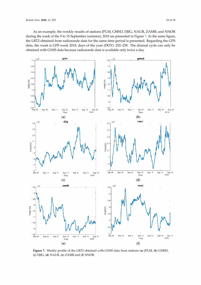
As an example, the weekly results of stations JPLM, GMSD, DJIG, NAUR, ZAMB, and NNORduring the week of the 9 to 15 September (autumn), 2018 are presented in Figure 7. In the same figure,the LRT2 obtained from radiosonde data for the same time period is presented. Regarding the GPSdata, the week is GPS week 2018, days of the year (DOY): 252–258. The diurnal cycle can only beobtained with GNSS data because radiosonde data is available only twice a day.

Remote Sens. 2020, 12, x FOR PEER REVIEW 10 of 18

3.3. Results of Proposed Algorithm

GNSS data is available every 30 seconds every day of the year for most of the stations presented in Table 1. However, in some cases, some data is missing. All available GNSS data of the selected stations and periods was processed to test the algorithm. Daily, there are 2880 epochs of data, which were processed with RTKLIB. Each processed epoch produced a value for ZTD and for zsite, which were used to test the proposed algorithm. The results are presented at three different time frames; first, one week in the month of July for two stations are presented as an example of how the results can be used to study the diurnal cycle of the height of the tropopause. Second, the yearly profile of the height of the tropopause obtained with the algorithm is shown for two stations as an example. Finally, the height of LRT1 and LRT2 obtained from radiosonde data and from the algorithm are shown for all latitudes.

As an example, the weekly results of stations JPLM, GMSD, DJIG, NAUR, ZAMB, and NNOR during the week of the 9 to 15 September (autumn), 2018 are presented in Figure 7. In the same figure, the LRT2 obtained from radiosonde data for the same time period is presented. Regarding the GPS data, the week is GPS week 2018, days of the year (DOY): 252–258. The diurnal cycle can only be obtained with GNSS data because radiosonde data is available only twice a day.

(a) (b)

(c) (d)

Remote Sens. 2020, 12, x FOR PEER REVIEW 11 of 18

(e) (f)

Figure 7. Weekly profile of the LRT2 obtained with GNSS data from stations (a) JPLM, (b) GMSD, (c) DJIG, (d) NAUR, (e) ZAMB and (f) NNOR.

Figure 7 shows the diurnal cycle of the height of the tropical tropopause obtained with GNSS data and the algorithm presented in the previous section. In all stations, during the week, rapid variations of the height of the tropopause can be seen. For some days, there is a clear diurnal cycle: at the beginning of the day, the height is higher than at the end of the day. However, some days exhibit more chaotic variation, and the diurnal cycle is less obvious.

Figure 8 shows the annual profile of the height of LRT2 for stations JPLM, GMSD, DJIG, NAUR, ZAMB, and NNOR obtained with GNSS data and the presented algorithm.

(a) (b)

(c) (d)

Figure 7. Weekly profile of the LRT2 obtained with GNSS data from stations (a) JPLM, (b) GMSD,(c) DJIG, (d) NAUR, (e) ZAMB and (f) NNOR.

Remote Sens. 2020, 12, 293 11 of 18

Figure 7 shows the diurnal cycle of the height of the tropical tropopause obtained with GNSS dataand the algorithm presented in the previous section. In all stations, during the week, rapid variations ofthe height of the tropopause can be seen. For some days, there is a clear diurnal cycle: at the beginningof the day, the height is higher than at the end of the day. However, some days exhibit more chaoticvariation, and the diurnal cycle is less obvious.

Figure 8 shows the annual profile of the height of LRT2 for stations JPLM, GMSD, DJIG, NAUR,ZAMB, and NNOR obtained with GNSS data and the presented algorithm.

Remote Sens. 2020, 12, x FOR PEER REVIEW 11 of 18

(e) (f)

Figure 7. Weekly profile of the LRT2 obtained with GNSS data from stations (a) JPLM, (b) GMSD, (c) DJIG, (d) NAUR, (e) ZAMB and (f) NNOR.

Figure 7 shows the diurnal cycle of the height of the tropical tropopause obtained with GNSS data and the algorithm presented in the previous section. In all stations, during the week, rapid variations of the height of the tropopause can be seen. For some days, there is a clear diurnal cycle: at the beginning of the day, the height is higher than at the end of the day. However, some days exhibit more chaotic variation, and the diurnal cycle is less obvious.

Figure 8 shows the annual profile of the height of LRT2 for stations JPLM, GMSD, DJIG, NAUR, ZAMB, and NNOR obtained with GNSS data and the presented algorithm.

(a) (b)

(c) (d) Remote Sens. 2020, 12, x FOR PEER REVIEW 12 of 18

(e) (f)

Figure 8. Annual profile of the height of LRT2 obtained with GNNS data from station (a) JPLM, (b) GMSD, (c) DJIG, (d) NAUR, (e) ZAMB, and (f) NNOR.

According to Figure 8a–f, Stations JPLM and GMSD follow the same pattern because they are further away from the equator. During the summer months, the height of LRT2 is minimum. Station NAUR shows a very small variation, i.e., the height of LRT2 seems to be constant except for three peaks. Station NAUR is located in Nauru, which is on the equator; therefore, the height of LRT2 is expected to be higher than other locations and the weather to be almost constant. Station NNOR is south of the equator; therefore, the maximum values for the height of LRT2 are found during the summer. The behavior is the opposite to that of stations north of the equator.

Equation (6) is applied to estimate the height of the tropical tropopause using GNSS data; however, radiosonde data is also used for validation purposes. The height of the tropical tropopause measured using annual GNSS and radiosonde data is shown in Figure 9.

Figure 9. Height of LRT2 obtained with radiosonde and GNSS data.

Figure 9 shows the height of LRT2 obtained with radiosonde and with GNSS data. The LRT2 was calculated using the algorithm previously described with GNSS data and applying the WMO’s definition of the LRT2 to the radiosonde soundings in the stations described in Table 2. Every day, there are 2880 epochs of GNSS data. Therefore, a daily average is calculated; these daily averages are themselves averaged to find a single value at a given station in a year, which is plotted in Figure 9.

Figure 8. Annual profile of the height of LRT2 obtained with GNNS data from station (a) JPLM, (b)GMSD, (c) DJIG, (d) NAUR, (e) ZAMB, and (f) NNOR.

Remote Sens. 2020, 12, 293 12 of 18

According to Figure 8a–f, Stations JPLM and GMSD follow the same pattern because they arefurther away from the equator. During the summer months, the height of LRT2 is minimum. StationNAUR shows a very small variation, i.e., the height of LRT2 seems to be constant except for three peaks.Station NAUR is located in Nauru, which is on the equator; therefore, the height of LRT2 is expected tobe higher than other locations and the weather to be almost constant. Station NNOR is south of theequator; therefore, the maximum values for the height of LRT2 are found during the summer. Thebehavior is the opposite to that of stations north of the equator.

Equation (6) is applied to estimate the height of the tropical tropopause using GNSS data; however,radiosonde data is also used for validation purposes. The height of the tropical tropopause measuredusing annual GNSS and radiosonde data is shown in Figure 9.

Remote Sens. 2020, 12, x FOR PEER REVIEW 12 of 18

(e) (f)

Figure 8. Annual profile of the height of LRT2 obtained with GNNS data from station (a) JPLM, (b) GMSD, (c) DJIG, (d) NAUR, (e) ZAMB, and (f) NNOR.

According to Figure 8a–f, Stations JPLM and GMSD follow the same pattern because they are further away from the equator. During the summer months, the height of LRT2 is minimum. Station NAUR shows a very small variation, i.e., the height of LRT2 seems to be constant except for three peaks. Station NAUR is located in Nauru, which is on the equator; therefore, the height of LRT2 is expected to be higher than other locations and the weather to be almost constant. Station NNOR is south of the equator; therefore, the maximum values for the height of LRT2 are found during the summer. The behavior is the opposite to that of stations north of the equator.

Equation (6) is applied to estimate the height of the tropical tropopause using GNSS data; however, radiosonde data is also used for validation purposes. The height of the tropical tropopause measured using annual GNSS and radiosonde data is shown in Figure 9.

Figure 9. Height of LRT2 obtained with radiosonde and GNSS data.

Figure 9 shows the height of LRT2 obtained with radiosonde and with GNSS data. The LRT2 was calculated using the algorithm previously described with GNSS data and applying the WMO’s definition of the LRT2 to the radiosonde soundings in the stations described in Table 2. Every day, there are 2880 epochs of GNSS data. Therefore, a daily average is calculated; these daily averages are themselves averaged to find a single value at a given station in a year, which is plotted in Figure 9.

Figure 9. Height of LRT2 obtained with radiosonde and GNSS data.

Figure 9 shows the height of LRT2 obtained with radiosonde and with GNSS data. The LRT2was calculated using the algorithm previously described with GNSS data and applying the WMO’sdefinition of the LRT2 to the radiosonde soundings in the stations described in Table 2. Every day,there are 2880 epochs of GNSS data. Therefore, a daily average is calculated; these daily averages arethemselves averaged to find a single value at a given station in a year, which is plotted in Figure 9.There are two radiosonde soundings every day. Therefore, a daily average of the obtained height ofLRT2 is calculated and plotted per station in Figure 9.

3.4. Validation of Results

Validation of the algorithm was done by comparing the results of LRT2 obtained with GNSS andradiosonde data. The results are shown in Figure 9. The differences of 1.4 km between 30◦S and 30◦Nwith a 95% confidence interval were obtained by doing a P-value test. Data from radiosondes wereaveraged and a single value per day was used. Figure 10 shows the residuals of the comparison ofLRT2 obtained with GNSS and radiosonde data.

Remote Sens. 2020, 12, 293 13 of 18

Remote Sens. 2020, 12, x FOR PEER REVIEW 13 of 18

There are two radiosonde soundings every day. Therefore, a daily average of the obtained height of LRT2 is calculated and plotted per station in Figure 9.

3.4. Validation of Results

Validation of the algorithm was done by comparing the results of LRT2 obtained with GNSS and radiosonde data. The results are shown in Figure 9. The differences of 1.4 km between 30°S and 30°N with a 95% confidence interval were obtained by doing a P-value test. Data from radiosondes were averaged and a single value per day was used. Figure 10 shows the residuals of the comparison of LRT2 obtained with GNSS and radiosonde data.

Figure 10. Residuals of the comparison of LRT2 obtained with GNSS and RS data.

Table 3 shows the height of LRT2 measured with radiosonde and GNSS data from the year 2018 (LRT2_RS and LRT2_GNSS). Also, the mean of the differences, the standard deviation, the maximum and minimum values, the median, and the RMSE of the differences are shown in Table 3 for validation purposes.

Figure 10. Residuals of the comparison of LRT2 obtained with GNSS and RS data.

Table 3 shows the height of LRT2 measured with radiosonde and GNSS data from the year2018 (LRT2_RS and LRT2_GNSS). Also, the mean of the differences, the standard deviation, themaximum and minimum values, the median, and the RMSE of the differences are shown in Table 3 forvalidation purposes.

Remote Sens. 2020, 12, 293 14 of 18

Table 3. Values of LRT1 and LRT2 obtained with radiosonde data and LRT2 obtained with GNSS data A1, LRT1_GNSS, and dLRT1.

Station Latitude[◦]

LRT2_RS[km]

LRT2_GNSS[km]

Mean_dlrt2[km]

STD_DLRT2[km]

dlrt2_Max[km]

dlrt2_Min[km]

Median_dlrt2[km]

RMSE[km]

JPLM 35 17.6 17.25 0.35 3.16 10.18 −6.76 −0.50 3.16GMSD 30 17.9 18.79 −0.89 3.36 12.42 −6.66 −0.31 3.37TWTF 25 18 19.53 −1.53 2.56 10.52 −6.00 −0.10 2.57MKEA 20 18 19.72 −1.72 2.36 6.30 −1.74 0.21 2.09CNMR 15 18.1 19.81 −1.71 1.98 10.12 −2.56 0.44 1.24DJIG 10 18.5 19.91 −1.41 1.69 5.96 −3.20 0.57 1.84

KOUG 5 19 19.95 −0.95 1.00 7.54 −0.12 1.68 2.50NAUR 0 19 20.36 −1.36 2.12 10.52 −0.99 2.30 3.36SEYG −5 18.9 19.70 −0.80 2.30 12.42 −0.12 2.08 2.99XMIS −10 18.5 17.95 0.55 2.40 6.30 −1.21 1.89 3.13

ZAMB −15 18.1 19.22 −1.12 2.31 9.62 −2.15 1.57 3.28VACS −20 18 19.30 −1.30 2.01 10.12 −1.99 0.54 2.51UFPR −25 17.8 18.59 −0.79 2.00 12.42 −0.88 0.34 2.00

NNOR −30 17.7 17.55 0.15 2.30 7.31 −4.05 0.13 2.34STR1 −35 17.7 19.33 −1.63 3.10 5.96 −1.10 −0.14 3.10

Remote Sens. 2020, 12, 293 15 of 18

4. Discussion of Results

GNSS data can be used to calculate the height of LRT2 and LRT1. Furthermore, it is possible todetect the diurnal cycle of the height of LRT2. The results in Figure 7 show the diurnal cycle of theheight of the tropopause found with GNSS data and the algorithm presented in this paper. StationsJPLM and GSMD are located at latitudes 35◦ and 30◦ north of the equator. For both stations, during themorning, the values were higher than during the afternoon. That’s the reason why a peak was foundat the beginning of the day. The average height found for JPLM was 13.4 km, while for GSMD, it was16.5 km, as expected, because latitudes closer to the equator have higher values for the height of LRT2.

Stations DJIG and NAUR are closer to the equator: DJIG is located at latitude 10◦ and NAUR ison the equator. Figure 7c,d show that the values for the height of LRT2 are bigger for NAUR thanfor DJIG because, according to previous research, the highest values of height of LRT2 are found atthe equator. The profile of diurnal cycle shows a little change between heights in one day. StationsZAMB and NNOR are represented in Figure 7e,f respectively. Both stations are south of the equator, atlatitudes of −15◦ and −30◦ respectively. The maximum values were found during the afternoon ratherthan in the morning. As expected, the heights were lower than those for the stations near the equator.

The heights of the LRT2 obtained with radiosonde and GNSS data for six stations are shown inFigure 8. Figure 8a−f show the annual profile of the height of the tropopause found with GNSS data.Figure 8a,b show the profile for stations JPLM and GSMD at latitude 35◦ and 30◦ north of the equator.In both cases, the minimum values were found during the summer months. The maximum valueswere found during the spring. GSMD lacks data from July and August 2018, but the tendency is clearfor lower values. The values for the height were lower at station JPLM than GSMD. Figure 8c,d showthe annual profile of the height of LRT2 at stations DJIG and NAUR, located at latitudes 10◦ and on theequator. As expected, the values for NAUR were the greater than those for all other stations becauseit is on the equator. Furthermore, the profile is almost flat. DJIG has bigger changes than NAUR;the maximum values for this latitude are found during the months of August and September, whichcorrespond to the summertime in the northern hemisphere.

Figure 8e,f show the annual profile of the height of LRT2 obtained with GNSS data at stationsin the southern hemisphere ZAMB (lat: −15◦) and NNOR (lat: −30◦). The profile at ZAMB has theopposite behavior to the profile of stations north of the equator. The maximum values were foundduring the months of February and March, which are the summer months in that hemisphere, and theminimum values were found in the months of August and September, which are the winter months inthe southern hemisphere. The values of the height of LRT2 at NNOR were smaller than for ZAMB, andthe profile showed small changes between the maximum and minimum values. The maximum valueswere found during June and July. In contrast, the minimum values were found during the months ofApril and May. The averaged values of LRT2 at different latitudes yielded the results presented inFigure 9, which show that the maximum values were found for stations closer to the equator with bothGNSS and radiosonde data.

Validation of the results was done by comparing the results obtained with radiosonde data andwith GNSS data. Both outcomes are shown in Figure 9. The quality of the results was evaluated withstatistical indicators. In Table 3, the following statistical indicators are shown: the average of thedifferences, the maximum and minimum values, the standard deviation of the differences, and themedian and the Root Mean Square Error of the differences. Furthermore, a P-value test found that thedifference in the 95% confidence interval for stations between −35◦ and 35◦ latitude is 2.7 km, whichis close to the resolution obtained using other techniques and data sources. Seven stations had anaverage difference of less than 1 km, five stations had an average difference between 1 and 2 km, andthe remaining three stations had an average difference between 2 km and 3 km. However, none ofthe stations had an average greater than 3 km. The discrepancies between the results are due to themodel of the e, and to errors in the estimation of ZTD, which are also linked to environmental variablesnot being accurately measured or estimated. Furthermore, missing radiosonde or GNSS data alsocontributed to the discrepancies.

Remote Sens. 2020, 12, 293 16 of 18

In order to reduce discrepancies, one year of data was processed so that different weatherconditions would be present, especially in the stations further away from the equator which havedifferent weather conditions through the year. Ten years of radiosonde data were processed to obtainthe equation here presented. The profile of the refractivity through the years changes very little;therefore, we used only one year of data to test the algorithm and assumed that in the other years, theresults would be similar. A limitation of the algorithm is that special weather conditions can increasethe discrepancies between the obtained height of the LRT2 with GNSS data and the measured LRT2from radiosonde data.

The advantage of the proposed technique is that the temporal resolution is increased. The ZTD canbe estimated with the PPP technique as frequently as the ephemeris and the GNSS data are available.In this case, there is a solution available every 30 seconds. Final precise ephemeris was used in our test;therefore, the solutions of the proposed algorithm is postprocessing with the latency of the availabilityof the final precise ephemeris product from IGS. Rapid precise ephemeris and improvements of thePPP technique towards real time would make the computation of ZTD possible in real time. Therefore,the height of LRT2 could be measured in real time. In contrast, the use of radiosonde data is limited bythe number of soundings, i.e., two per day in most radiosonde stations. Another advantage of theproposed algorithm is that it is possible to observe the diurnal cycle of the height of LRT2 at a higherresolution, because there are GNSS measurements throughout whole the day.

5. Conclusions

The Zenith Tropospheric Delay (ZTD) can be used to monitor the environment because of tworelationships, i.e., the relationship between the ZTD and the refractivity index of the troposphere (N),as defined using Equation (4), as well as the relationship between N and environmental variablessuch as temperature, water vapor partial pressure, and atmospheric pressure. Previously, algorithmshave been developed to monitor the water vapor and the precipitable water using ZTD. However, thisresearch showed that monitoring the height of the tropopause layer using the ZTD as input is alsopossible because of the relationship of the ZTD and the path of the signal which passes the tropopause.

The profile of refractivity was obtained with the measurements of pressure (p) and temperature(T) at different levels. It was assumed that the water vapor is distributed in the troposphere, so it wascalculated with the first temperature reported by the radiosonde; the same value was used at differentheights. The profile was fitted into an exponential function, and two values were found: N0 and Nh.Ten years of data were processed, and it was found that the profiles of N0 and Nh were periodical ateach latitude. Therefore, a single average value of N0 and Nh per latitude was obtained.

In this paper, we have presented an algorithm to calculate the height of the tropical tropopauseusing high-resolution GNSS data. The algorithm was tested using high-resolution GNSS data from15 stations between latitudes of 30◦S and 30◦N. The algorithm was validated using radiosonde datafrom stations in the same latitudes. It was found that the profile of refractivity against height isperiodical through the years. Also, it was found that the annual change of the values N0 and Nh arenegligible; therefore, those parameters can be calculated with data from a single year and applied todifferent years.

The profile of the height of the tropopause (LRT1 and LRT2) can be obtained with GNSS data, asshown in Figure 9. Validation was done by comparing the results obtained with GNSS and radiosondedata, and the definition of the WMO. It was found that the average difference between both results isless than 3 km for all stations; five stations yielded averaged differences of less than 1 km. Furthermore,it is shown in Figure 8 that it is possible to monitor the diurnal cycle of the height of the tropopauseusing GNSS data because it has a higher temporal resolution. The ZTD can be estimated from PPP at afrequency of 30 s. Therefore, the height of LRT2 can be estimated at the same frequency as the ZTD.

Author Contributions: Conceptualization: J.M.A. and L.L.; Data downloading and processing J.M.A.; Correlationanalysis and validation Y.-T.T.; Presentation of results including plots and tables: J.M.A. and L.L.; Algorithm

Remote Sens. 2020, 12, 293 17 of 18

validation and analysis: J.M.A., Y.-T.T., and T.M. Writing, review and editing, J.M.A., L.L., Y.-T.T., and T.M. Finalreview and editing L.L. and T.M. All authors have read and agreed to the published version of the manuscript.

Funding: This work was supported by financial support from the International Doctoral Innovation Centre,Ningbo Education Bureau, Ningbo Science and Technology Bureau, and the University of Nottingham. This workwas also supported by the UK Engineering and Physical Sciences Research Council [grant number [EP/L015463/1].

Conflicts of Interest: The authors declare no conflict of interest.

References

1. Santer, B.D.; Sausen, R.; Wigley, T.M.L.; Boyle, J.S.; AchutaRao, K.; Doutriaux, C.; Hansen, J.E.; Meehl, G.A.;Roeckner, E.; Ruedy, R.; et al. Behavior of tropopause height and atmospheric temperature in models,reanalyses, an d observations: Decadal changes. J. Geophys. Res. 2003, 108, 22. [CrossRef]

2. Santer, B.D.; Wehner, M.F.; Wigley, T.M.L.; Sausen, R.; Meehl, G.A.; Taylor1, K.E.; Ammann, C.; Arblaster, J.;Washington, W.M.; Boyle1, J.S.; et al. Contribution of anthropogenic and natural forcing to recent tropopauseheight changes. Sci. Mag. 2003, 301, 479–483. [CrossRef]

3. Santer, B.D.; Wigley, T.M.L.; Simmons, A.J.; Kållberg, P.W.; Kelly, G.A.; Uppala, S.M.; Ammann, C.;Boyle, J.S.; Brüggemann, W.; Doutriaux, C.; et al. Identification of anthropogenic climate change using asecond-generation reanalysis. J. Geophys. Res. 2004, 109, 1–19. [CrossRef]

4. Schmidt, T.; Beyerle, G.; Heise, S.; Wickert, J.; Rothaucher, M. A climatology of multiple tropopauses derivedfrom GPS radio occultations with CHAMP and SAC-C. Geophys. Res. Lett. 2006, 33. [CrossRef]

5. Holton, J.R.; Haynes, P.H.; McIntyre, M.E.; Douglass, A.R.; Rood, R.B.; Pfister, L. Stratosphere-TroposphereExchange. Rev. Geophys. 1995, 33, 403–439. [CrossRef]

6. Feng, S.; Fu, Y.; Xiao, Q. Trends in the global tropopause thickness revealed by radiosondes. Geophys. Res.Lett. 2012, 39. [CrossRef]

7. WMO. Meteorology: A three-dimensional science: Second session of the Commission for Aerology. WMOBull. 1957, 4, 134–138.

8. Seidel, D.J.; Randel, W.J. Variability and trends in the global tropopause estimated from radiosonde data. J.Geophys. Res. 2006, 111. [CrossRef]

9. Rieckh, T.; Scherllin-Pirscher, B.; Ladstädter, F.; Foelsche, U. Characteristics of tropopause parameters asobserved with GPS radio occultation. Atmos. Meas. Tech. 2014, 7, 2014–3958. [CrossRef]

10. Añel, J.A.; Gimeno, L.; de la Torre, L.; Nieto, R. Changes in tropopause height for the Eurasian regiondetermined from CARDS radiosonde data. Naturwissenschaften 2006, 93, 2006–2609. [CrossRef]

11. Hall, C.M.; Hansen, G.; Sigernes, F.; Ruiz, K.M.K. Tropopause height at 78N 16E: Average seasonal variation2007–2010. Atmos. Chem. Phys. 2011, 11, 2011–5490. [CrossRef]

12. Arai, K.; Liang, X.M. Sensitivity analysis for air temperature profile estimation methods around the tropopauseusing simulated Aqua/AIRS data. Adv. Space Res. 2009, 43, 2009–2851. [CrossRef]

13. Lerner, J.A.; Weisz, E.; Kirchengast, G. Temperature and humidity retrieval from simulated InfraredAtmospheric Sounding Interferometer (IASI) measurements. J. Geophys. Res. Atmos. 2002, 107, 1–11.[CrossRef]

14. Lau, L.; Cross, P. Phase Multipath Mitigation Techniques for High Precision Positioning in All Conditionsand Environments. J. Navig. 2007, 60, 457–482. [CrossRef]

15. Lau, L.; Tateshita, H.; Sato, K. Impact of Multi-GNSS on Positioning Accuracy and Multipath Errors inHigh-Precision Single-Epoch Solutions -A Case Study in Ningbo China. J. Navig. 2015, 68, 999–1017.[CrossRef]

16. Wang, B.; Miao, L.; Wang, S.; Shen, J. A constrained LAMBDA method for GPS attitude determination. GPSSolut. 2009, 13, 97–107. [CrossRef]

17. Lau, L.; Cross, P.; Steen, M. Flight Tests of Error-Bounded Heading and Pitch Determination with Two GPSReceivers. IEEE Trans. Aerosp. Electron. Syst. 2012, 48, 388–404. [CrossRef]

18. Awange, J.L. Environmental Monitoring Using GNSS: Global Navigation Satellite Systems; Springer:Berlin/Heidelberg, Germany, 2012.

19. Astudillo, J.M.; Lau, L.; Tang, Y.-T.; Moore, T. Analysing the Zenith Tropospheric Delay Estimates in On-linePrecise Point Positioning (PPP) Services and PPP Software Packages. Sensors 2018, 18, 580. [CrossRef][PubMed]

Remote Sens. 2020, 12, 293 18 of 18

20. Mathew, S.S.; Kumar, K. Estimation of zonally resolved edges of the tropical belt using GPS-RO measurements.IEEE J. Sel. Top. Appl. Earth Obs. Remote Sens. 2018, 11, 2555–2561. [CrossRef]

21. Hoinka, K.P. Statistics of the Global Tropopause Pressure. Mon. Weather Rev. 1998, 126, 3303–3325. [CrossRef]22. Hofmann-Wellenhof, B.; Lichtenegger, H.; Wasle, E. GNSS-Global Navigation Satellite Systems GPS, GLONASS,

GALILEO and More; Springer: Wien, Austria, 2008.23. Thayer, G. An improved equation for the radio refractive index of air. Radio Sci. 1974, 9, 803–807. [CrossRef]24. Essen, L.; Froome, K.D. The refractive indices and dielectric constants of air and its principal constituents at

24,000 Mc/s. Proc. Phys. Soc. Sect. B 1951, 64, 862. [CrossRef]25. Bevis, M.; Businger, S.; Herring, T.A.; Rocken, C.; Anthes, R.A.; Ware, R.H. GPS Meteorology: Remote Sensing

of Atmospheric Water Vapor Using the Global Positioning System. J. Geophys. Res. 1992, 97, 15787–15801.[CrossRef]

26. Thomson, G.W. The Antoine Equation for Vapor Pressure Data. Chem. Rev. 1946, 38, 1–39. [CrossRef]27. Gao, Y. GNSS Solutions: Precise Point Positioning and Its Challenges. InsideGNSS 2006, November/December,

16–18.28. Heroux, P.; Kouba, J. GPS Precise Point Positioning Using IGS Orbit Products. Phys. Chem. Earth 2001, 26,

573–578. [CrossRef]29. Zumberge, J.F.; Heflin, M.B.; Jefferson, D.C.; Watkins, M.M.; Webb, F.H. Precise point positioning for the

effcient and robust analysis of GPS data from large networks. Geophys. Res. 1997, 12, 5005–5017. [CrossRef]30. Tolman, B.W. GPS Precise Absolute Positioning via Kalman Filtering. In Proceedings of the ION GNSS 21st

International Technical Meeting of the Satellite Division, Savannah, GA, USA, 16–19 September 2008.31. Takasu, T. Real-time PPP with RTKLIB and IGS real-time satellite orbit and clock. In Proceedings of the IGS

Workshop 2010, Newcastle upon Tyne, UK, 28 June–2 July 2010.

© 2020 by the authors. Licensee MDPI, Basel, Switzerland. This article is an open accessarticle distributed under the terms and conditions of the Creative Commons Attribution(CC BY) license (http://creativecommons.org/licenses/by/4.0/).