A Note on the Symplectic Integration of theNonlinear Schrödinger Equation

Clemens Heitzinger and Christian Ringhofer

October 2003

Abstract

Numerically solving the nonlinear Schrödinger equation and be-ing able to treat arbitrary space dependent potentials permits manyapplication in the realm of quantum mechanics.

The long-term stability of a numerical method and its conservationproperties is an important feature since it assures that the underlyingphysics of the solution are respected and it ensures that the numericalresult is correct also for small time spans.

In this paper we describe symplectic integrators for the nonlin-ear Schrödinger equation with arbitrary potentials and perform nu-merical experiments comparing different approaches and highlight-ing their respective advantages and disadvantages.

1 Introduction

The motivation for considering the time-dependent Schrödinger equationand its solutions for large time spans stems from the fact that quantum-mechanical effects will play a dominating role in nano-scale semiconduc-tor devices and in new device concepts beyond traditional CMOS based onsilicon technology (e.g., single-electron devices and resonant-tunneling de-vices) [1]. Numerical schemes of this kind are also a prerequisite for thetransient simulation of proposed devices like quantum dots and quantumcellular automata [2, 3].

The wave equation or the time-dependent Schrödinger equation

ih∂ψ(r, t)

∂t= − h2

2m∇2ψ(r, t) + V0 · ψ(r, t)

1

describes the non-relativistic quantum mechanics for particles withoutspin. Here a particle of mass m moves in a field represented by the potentialenergy function V0. Scaling this equation yields the equations consideredin this work.

In the following we consider the Schrödinger equation in the form

iut + uxx + 2uV(t, x, u) = 0.

V(t, x, u) denotes the potential and in the case of the Schrödinger equationwith cubic nonlinearity in one space dimension it is of the form V(t, x, u) =|u|2 + V1(t, x), where V1(t, x) is an arbitrary real valued function. Moreprecisely, we are interested in numerical solutions of the initial boundaryvalue problem

u : [0, T]× [0, 1] → C

iut + uxx + 2uV(t, x, u) = 0u(0, x) givenperiodic boundary conditions for x ∈ [0, 1]

obtained by methods of geometric integration.A review of the analytical properties of the solutions of the cubic nonlin-

ear Schrödinger equation can be found in [4] which also discusses the con-nection of this PDE to dynamical systems. This nonlinear equation showsinteresting phenomena like solitary waves and solitons, finite-time blow-up, chaotic evolution in deterministic PDEs, and periodic waves and quasi-periodic wave-trains. It also has applications to nonlinear optics, laserdynamics, and photonics [5, 6]. Implementors of simulators for quantumdots and similar applications will be more interested in the equation withthe linear potential term, to which the same methods can be applied in astraightforward manner.

Runge–Kutta methods and linear multi-step methods for ODEs havereached a high level of maturity and are generally available program codes.Although Runge–Kutta methods can conserve linear and quadratic invari-ants, no Runge–Kutta method can conserve all polynomial invariants ofdegree three and higher [7]. This motivates the search for new methodswhich respect the geometric properties of the solutions.

The main idea of the geometric integration of ODEs and PDEs is that thegeometry of the equation to be solved should be respected by the numericalmethod, i.e., invariants of the equation are also conserved by the numericalintegrator [7–10].

2

The method of Poisson integrators, a generalization of symplectic in-tegrators, will be used to derive implicit finite difference schemes for theproblem above. The paper is organized into an introduction to symplecticintegrators for Hamiltonian systems in Section 2, a recapitulation of Pois-son integrators and their application to the initial boundary value problemin Section 3 and Section 4, and finally several numerical results for the non-linear Schrödinger equation are presented in Section 5.

2 Symplectic Integrators

We start by defining the notion of symplectic (i.e., area preserving) func-tions. A linear function is defined to be symplectic if it conserves orientedarea as defined by the parallelogram spanned by two vectors. Hence a dif-ferentiable function is called symplectic if its Jacobian is everywhere sym-plectic.

There is an interesting connection between symplectic functions andHamiltonian systems, i.e., systems of the form

p = −∇qH(p, q)q = ∇pH(p, q),

where p and q are vectors denoting momentum and position, respectively.H(p, q) is the Hamiltonian and a first integral of the system. The followingtheorem is due to Poincaré [7, 11].

Theorem 2.1 Let H(p, q) be a twice continuously differentiable function onU ⊂ R2d defining a Hamiltonian system. Then the flow ϕt of the Hamiltoniansystem (i.e., the mapping that advances the solution by time) is a symplectic trans-formation (wherever it is defined) for all t.

The converse is also true:

Theorem 2.2 Let f : U → R2d be a continuously differentiable function. Thenthe system y = f (y) is locally Hamiltonian (i.e., it can locally be written in theform of a Hamiltonian system) if and only if its flow ϕt(y) is symplectic for ally ∈ U and for all sufficiently small t.

Because of the characteristic symplectic nature of the flow of a Hamil-tonian system, it is natural to search for numerical methods sharing thisproperty. Hence we extend the definition of symplecticity to numericalone-step methods.

3

Definition 2.3 A numerical one-step method is called symplectic, if the one-step map yn+1 = Φh(yn) is symplectic whenever the method is applied to asmooth Hamiltonian system.

Examples of symplectic one-step methods are the symplectic Eulerscheme

pn+1 = pn − h∂H∂q

(pn+1, qn)

qn+1 = qn + h∂H∂p

(pn+1, qn)

which is of order 1. The same holds for its adjoint method

pn+1 = pn − h∂H∂q

(pn, qn+1)

qn+1 = qn + h∂H∂p

(pn, qn+1).

The implicit mid-point rule

pn+1 = pn − h∂H∂q

((pn+1 + pn)/2, (qn+1 + qn)/2

)qn+1 = qn + h

∂H∂p

((pn+1 + pn)/2, (qn+1 + qn)/2

)is a symplectic method of order 2. Furthermore compositions of symplec-tic methods are again symplectic methods, which is one way to constructhigher-order symplectic schemes.

Examples of symplectic Gauss collocation (or Runge–Kutta) methodsare the following. If s is the degree of the collocation polynomial, then theGauss collocation methods are of order 2s. For s = 1 we again have theimplicit midpoint rule

1/2 1/21

, (1)

and the methods for s = 2 (order 4) and s = 3 (order 6) are shown in Table 2.The conservation property of symplectic methods is condensed in the

following important result obtained by backward error analysis [7, 12]. Af-ter truncation, the modified Hamiltonian is

H(y) = H(y) + hmHm+1(y) + · · ·+ hN−1HN(y),

where m is the order of the method.

4

1/2−√

3/6 1/4 1/4−√

3/61/2 +

√3/6 1/4 +

√3/6 1/4

1/2 1/2

1/2−√

15/10 5/36 2/9−√

15/15 5/36−√

15/301/2 5/36 +

√15/24 2/9 5/36−

√15/24

1/2 +√

15/10 5/36 +√

15/30 2/9 +√

15/15 5/365/18 4/9 5/18

Table 1: Butcher tableaus of Gauss collocation methods of order 4 and 6.

Theorem 2.4 (Long Term Energy Conservation) If a symplectic numericalmethod of order m with step size h is applied to a Hamiltonian system with an-alytic H : D → R (where D ⊂ R2d) and the numerical solution remains in acompact set K ⊂ D, then there are h0 and N(h) such that

H(yn) = H(y0) + O(e−h0/2h)H(yn) = H(y0) + O(hm)

over exponentially long time intervals nh ≤ eh0/2h.

It is one of the favorable properties of symplectic methods that these equa-tions hold for exponentially long time intervals. For a non-symplecticmethod the second equation would generally read H(yn) = H(y0) +O(nhm) meaning that the error would generally increase linearly with time.

3 Poisson Integrators

Unfortunately many systems of practical importance, especially those forquantum-mechanical systems, cannot be written as Hamiltonian systems.Generalizing the ideas from Section 2 to systems of the form

y = P(y)∇H(y), (2)

where P(y) is a Poisson bracket, leads to Poisson integrators. In the previ-ous section we had y = (p, q) and P(y) = J−1, where

J :=(

0 I−I 0

)(3)

and I is the identity matrix. In this section we summarize the generalizationto more general P(y). It is based on the Darboux–Lie Theorem and henceclassic work by Clebsch, Darboux, Jacobi, and Lie [7, 13–16].

5

We start with some definitions.

Definition 3.1 (Poisson Bracket) Let P(y) = pij(y) (i, j ∈ {1, . . . , n}) be asmooth matrix-valued function. If

{F, G}(y) := ∇F(y)TP(y)∇G(y) =n

∑i=1

n

∑j=1

∂F(y)∂yi

pij(y)∂G(y)

∂yj

is bilinear, skew-symmetric ({F, G} = −{G, F}), and satisfies Leibniz’s rule

{F · G, H} = F · {G, H}+ G · {F, H}

and the Jacobi identity{{F, G}, H

}+

{{H, F}, G

}+

{{G, H}, F

}= 0

for sufficiently smooth F, G, and H, then {F, G}(y) is called the Poissonbracket of F and G.

Definition 3.2 (Poisson System) If P(y) represents a Poisson bracket, then

y = P(y)∇H(y)

is called a Poisson system. Again H is called the Hamiltonian.

Lemma 3.3 P(y) represents a Poisson bracket if and only if P(y) is a skew-symmetric matrix and the condition ∀∀∀i, j, k :

n

∑ν=1

(∂pij(y)

∂yνpνk(y) +

∂pjk(y)∂yν

pνi(y) +∂pki(y)

∂yνpνj(y)

)= 0

for the Jacobi identity is satisfied. (Because of the structure of the Poisson bracketas a sum it is always bilinear and and always satisfies Leibniz’s rule.)

It is trivial to check that J defined in (3) indeed represents a Poisson bracket.The Darboux–Lie Theorem answers the question which coordinate

transformation of a Poisson system yields the simplest possible form – orcanonical form – of P(y).

Definition 3.4 (Canonical Form) A Poisson system represented by P(y) issaid to be in canonical form if it is of the form

P(y) =(

J−1 00 0

).

6

Theorem 3.5 (Darboux–Lie) Let P(y) represent a Poisson system. If P(y)is of constant rank n − r = 2m in a neighborhood of y0 ∈ Rn, then thereare functions P1(y), . . . , Pm(y), Q1(y), . . . , Qm(y), and (the so-called Casimirs)C1(y), . . . , Cr(y) so that

{Pi, Pj} = 0 {Pi, Qj} = −δij {Pi, Cl} = 0

{Qi, Pj} = δij {Qi, Qj} = 0 {Qi, Cl} = 0

{Ck, Pj} = 0 {Ck, Qj} = 0 {Ck, Cl} = 0

holds in a neighborhood of y0. The gradients of Pi, Qi, and Ck are linearly inde-pendent and hence y 7→

(Pi(y), Qi(y), Ck(y)

)is a local change of coordinates to

canonical form.

The proof is constructive and, roughly speaking, works by iterating overthe rows and columns of the structure matrix to find suitable coordinates Piand Qi as solutions of linear PDEs.

Important properties of Hamiltonian systems are also true for Poissonsystems. First the Hamiltonian of the Poisson system is again a first inte-gral. Analogously to symplectic maps, it is possible to define Poisson maps.Then in analogy to Theorem 2.1 it can be proven under certain smoothnessassumptions that a system is locally a Poisson system, whose structure ma-trix is a Poisson bracket, if and only if its flow is a Poisson map and respectsthe Casimirs of the transformation of the Poisson bracket to canonical form.Again, as in the case of Definition 2.3, this motivates the following defini-tion.

Definition 3.6 A numerical one-step method is called a Poisson integratorfor a Poisson system with structure matrix P(y), if the one-step map yn+1 =Φh(yn) is a Poisson map whenever it is applied to the Poisson system andif Φh respects the Casimirs of the transformation of P(y) to canonical form.

Clearly a numeric integrator can only be a Poisson integrator for certainstructure matrices P(y).

Table 2 summarizes how the concepts for Hamiltonian systems, i.e., sys-tems with canonical Poisson bracket, and systems with general Poissonbracket relate to one another. These considerations give rise to a Poissonintegrator for Poisson systems. In summary it consists of the followingsteps:

1. First find the transformation ϕ(y) :=(

Pi(y), Qi(y), Ck(y))

to canoni-cal form for the given structure matrix P(y) by using Theorem 3.5.

7

Hamiltonian system Poisson systemCanonical form General Poisson bracketSymplectic transformation Poisson mapFlow is symplectic Flow is a Poisson map

and respects the CasimirsSymplectic integrator Poisson integrator

Table 2: The column on the left hand side lists some concepts for Hamiltoniansystems and the corresponding concepts for general Poisson systems are shownon the right hand side. The transformation to canonical Poisson form allows totranslate between these two.

2. Define zn := ϕ(yn) and apply a symplectic integrator to the trans-formed system which has now a structure matrix in canonical form(cf. Definition 3.4).

3. Transform back to the original coordinates yn = ϕ−1(zn).

4 Poisson Integrators for the Nonlinear SchrödingerEquation

We now carry out the ideas of the previous sections for the nonlinear equa-tion in its most general form

iut + uxx + 2αu(|u|2 + V1(t, x)

)= 0

for periodic boundary conditions. V1 is a real valued function and α ∈R\{0}. Depending on how the nonlinear term is discretized, one can writethe system in Hamiltonian form in straightforward manner (u 7→ wk, Sec-tion 4.1) or one arrives at the Ablowitz–Ladik model (2u 7→ wk−1 + wk+1,Section 4.2).

4.1 A Hamiltonian for the Canonical Form

Discretizing the derivations with respect to the space variable first in anequidistant manner, we obtain the equations

i∂wk

∂t+

wk+1 − 2wk + wk−1

∆x2 + 2αwk(|wk|2 + V1(t, x)

)= 0

8

in the new variables wk, k ∈ {1, . . . , N}. In the next step we split the newvariables wk into real and imaginary parts via wk = uk + ivk. This yields

∂uk

∂t= − 1

∆x2 (vk+1 − 2vk + vk−1)− 2αvk(u2k + v2

k + V1(t, x))

∂vk

∂t= 1

∆x2 (uk+1 − 2uk + uk−1) + 2αuk(u2k + v2

k + V1(t, x)).

Introducing the notation u := (u1, . . . , uN) and v := (v1, . . . , vN) and defin-ing the Hamiltonian

H(u, v) :=1

∆x2

N

∑k=1

(ukuk−1 − u2k + vkvk−1 − v2

k) +α

2

N

∑k=1

(u2

k + v2k + V1(t, x)

)2

we obtain(uv

)=

(0 −II 0

) (∇uH(u, v)∇vH(u, v)

)and have thus written the system in canonical form.

4.2 A Transformation for the Ablowitz–Ladik Model

To arrive at the Ablowitz-Ladik model, we now discretize the nonlinearterm using 2u 7→ wk−1 + wk+1 [17, 18] and obtain

i∂wk

∂t+

wk+1 − 2wk + wk−1

∆x2 + α(wk−1 + wk+1)(|wk|2 + V1(t, x)

)= 0

in the new variables wk, k ∈ {1, . . . , N}. Again we split the new variableswk into real and imaginary parts via wk = uk + ivk. This yields

∂uk

∂t= − 1

∆x2 (vk+1 − 2vk + vk−1)− α(vk+1 + vk−1)(u2k + v2

k + V1(t, x))

∂vk

∂t= 1

∆x2 (uk+1 − 2uk + uk−1) + α(uk+1 + uk−1)(u2k + v2

k + V1(t, x)).

We can write these equations in the form of (2). Introducing the notationu := (u1, . . . , uN) and v := (v1, . . . , vN) we obtain(

uv

)=

(0 −DD 0

) (∇uH(u, v)∇vH(u, v)

),

where the entries of the diagonal matrix D are

dk := 1 + α∆x2(u2k + v2

k + V1(t, x))

9

and

H(u, v) :=1

∆x2

N

∑k=1

(ukuk−1 + vkvk−1)

− 1α∆x4

N

∑k=1

ln(1 + α∆x2(u2

k + v2k + V1(t, x))

).

Checking the conditions from Definition 3.1 via Lemma 3.3 is straightfor-ward. (This is in fact true for all systems where P(y) has the structure

P(y) =(

0 −DD 0

)(4)

with D being a diagonal matrix.) Fortunately this system is a Poisson sys-tem (Definition 3.2) and the theory of Section 3 can be applied.

The transformation to canonical form is not unique and will generallydepend on V1, since dk depends on V1. However, the transformation tocanonical form should be global, i.e., it should be identical for all time steps;otherwise poor performance as time progresses has to be expected [7].Therefore we assume in the following that V1(t, x) vanishes.

In order to find a transformation to canonical form, we have to em-ploy Theorem 3.5 and set y := (p1, . . . , pN , q1, . . . , qN). For our P(y), theconventional procedure is to define Q1(y) := y1 and solve the linear PDE

{Q1, P1} = 1. This yields the transformation given in [19] for a transformedSchrödinger equation, which does not treat the variables u and v symmet-rically.

Because of dk(u, v) = dk(v, u) and H(u, v) = H(v, u) it is desirable tofind a transformation so that the relations pk(u, v) = pk(v, u) and qk(u, v) =qk(v, u) hold for the new variables pk and qk . We also use the ansatz P1 =P1(y1, yN+1) and Q1 = Q1(y1, yN+1) which is equivalent to pk = pk(uk, vk)and qk = qk(uk, vk). Due to the special structure (4) of P(y), we have r = 0in Theorem 3.5 and it can be verified that are the conditions {Pi, Pj} = 0and {Qi, Qj} = 0 of Theorem 3.5 are always fulfilled for structure matricesof this form. Therefore we have to find symmetric solutions of {Q1, P1} = 1which is equivalent to

−∂Q1

∂y1

∂P1

∂yN+1+

∂Q1

∂yN+1

∂P1

∂y1=

1dk

=1

1 + α∆x2(y21 + y2

N+1).

The right hand side suggests the substitution z := α∆x2(y21 + y2

N+1). Thesimple ansatz P1 = y1σ(z) and Q1 = yN+1σ(z) leads to the ODE

σ2 + 2zσσ′ =1

1 + z

10

which has the solution

σ(x) :=

√ln(1 + x)

x.

Hence we arrive at the transformation

pk := ukσ(α∆x2(u2

k + v2k)

)qk := vkσ

(α∆x2(u2

k + v2k)

),

which was also proposed in [7]. Its inverse transformation is

uk = pkτ(α∆x2(p2

k + q2k)

)vk = qkτ

(α∆x2(p2

k + q2k)

),

where

τ(x) :=

√ex − 1

x.

The inverse is found by observing that

α∆x2(p2k + q2

k) = ln(1 + α∆x2(u2

k + v2k)

)and

eα∆x2(p2k+q2

k) − 1 = α∆x2(u2k + v2

k),

which leads to

eα∆x2(p2k+q2

k) − 1α∆x2(p2

k + q2k)

2=

α∆x2(u2k + v2

k)ln

(1 + α∆x2(u2

k + v2k)

)and thus

τ(α∆x2(p2

k + q2k)

)=

1σ(α∆x2(u2

k + v2k)

) .

Therefore we have uk = pk/σ(α∆x2(u2

k + v2k)

)= pkτ

(α∆x2(p2

k + q2k)

)and

analogously vk = qk/σ(α∆x2(u2

k + v2k)

)= qkτ

(α∆x2(p2

k + q2k)

).

11

After the transformation the new Hamiltonian H in the variables pand q reads

H(p, q) =1

∆x2

N

∑k=1

τ(α∆x2(p2

k + q2k)

)τ(α∆x2(p2

k−1 + q2k−1)

)(pk pk−1 + qkqk−1)

− 1α∆x4

N

∑k=1

ln(eα∆x2(p2

k+q2k) + α∆x2V1(t, x)

).

Symplectic schemes can now be applied to this Hamiltonian as describedin Section 3.

5 Numerical Results

We use the numeric integrators to simulate physical situations of interest.The first example is a recurrence similar to those recently observed in op-tical fibers. The second one is a soliton hitting a sidewall potential. In thefirst example we compare the two Hamiltonian based methods from Sec-tion 4.

The symplectic methods from Section 2 are implicit. In the followingexamples experience showed that fixed-point iteration yields much betterresults than Newton methods, and hence fixed-point iteration was used toobtain all of the numerical results.

5.1 A Recurrence

Recently, an optical Fermi–Pasta–Ulam recurrence [20] was demonstratedexperimentally in an optical fiber [5, 6]. In this example we consider theequation with α := 1. We start from the initial condition u(0, x) := π

√2(1 +

110 cos(πx)

)and use periodic boundary conditions for x ∈ [−1, 1]. The

symplectic scheme for solving the ODE is the sixth order Gauss collocationmethod (Table 2) and N := 50.

Using the scheme from Section 4.1 we obtain the solution shownin Figure 1. The value of the mass varies between approximately39.675809692379175 and 39.67580969237926 and is well-conserved. Thesame is true for the Hamiltonian from Section 4.1, which varies betweenapproximately 10009.181417277767 and 10009.18141727789.

The scheme from Section 4.2 results in the solution shown in Fig-ure 2. The notable variation in mass is shown in Figure 3. The Hamilto-nian from Section 4.2 is well-conserved and stays between approximately9793.991350824712 and 9793.99135082576.

12

10

20

30

40

50

t10

20

30

40

50

x

0

5

10

15

10

20

30

40

50

t

Figure 1: The absolute value of the solution found using the direct method fort ∈ [0, 1] and ∆t := 5 · 10−6.

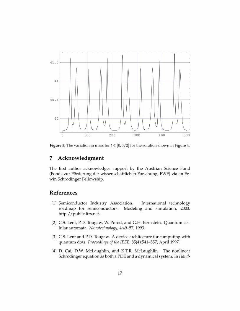
For reference Figure 4 shows the solution found by a first-same-as-lastembedded pair of explicit Runge–Kutta methods of order 6 using auto-matic time-step control. The notable variation in mass is shown in Figure 5.The Hamiltonian (Section 4.2) is well-conserved and lies between approxi-mately 9793.989394666394 and 9793.991573444684.

The analytic solution is unstable. The smallest perturbations result inlarge differences and this explains why the two solutions obtained fromthe two symplectic schemes (Figure 1 and Figure 2) show different behav-ior. Interestingly, mass is not conserved by the scheme from Section 4.2 asillustrated in Figure 3.

13

10

20

30

40

50

t10

20

30

40

50

x

0

5

10

10

20

30

40

50

t

Figure 2: The absolute value of the solution found using the transformation tocanonical form for t ∈ [0, 1/2] and ∆t := 5 · 10−6.

5.2 A Soliton Hitting a Sidewall Potential

In this section we consider the nonlinear Schrödinger equation with α :=1/2. Then a family of soliton solutions for x ∈ R is given by

u(t, x) := β sechβ(x − ct)√

2eic(x−ct)/2+iγt,

where c ∈ R is the speed of the soliton and γ ∈ R a parameter so thatβ2 := 2(γ− c2/4) has a positive solution for β.

In this example we chose V(x) := 1000 ·Heaviside(x− 5) as the outsidepotential, x ∈ [−5, 10], N := 100, and ∆t := 1/2000. In total 40 000 timesteps were performed for t ∈ [0, 20]. For solving the ODE we used the sixthorder Gauss collocation method (Table 2). The soliton is given by c := 1/2and γ := 10.

14

0 100 200 300 400 500

40

40.5

41

41.5

Figure 3: The variation in mass for t ∈ [0, 1/2] for the solution shown in Figure 2.

Figures 6 and 7 show the real and imaginary part of the solution, re-spectively, as found by the scheme from Section 4.1. The scheme fromSection 4.2 is not applicable, since the transformation to canonical Pois-son form is not possible where the initial conditions are sufficiently close tozero.

Table 3 compares mass conservation using double-precision floatingpoint numbers (about 16 digits). The mass difference between initial andfinal time step is Msymplectic(20)− M(0) ≈ −7.1 · 10−15.

The second column shows the mass of several time steps of a solutionobtained by a first-same-as-last embedded pair of explicit Runge–Kuttamethods of order 6 using automatic time-step control. The change in massis considerable.

6 Conclusion

Symplectic numerical methods are interesting because of their conservationproperties and their long-term stability for exponentially long time spans.When applying these methods to PDEs, it is however not obvious how towrite the ODE system obtained by the method of lines as a Hamiltonian

15

10

20

30

40

50

t10

20

30

40

50

x

5

10

10

20

30

40

50

t

Figure 4: The absolute value of the solution found using a nonsymplectic schemefor t ∈ [0, 3/2].

system. It may not be possible to write it as a Hamiltonian system or theform as a Hamiltonian or Poisson system is not unique. Furthermore in thecase of a Poisson system, the choice of the transformation to canonical formmay influence the numerical results as well.

Symplectic numerical schemes were given for the nonlinear Schrödin-ger equation with a cubic nonlinearity. The nonlinear term of the equationmay contain a arbitrary space and time dependent potential.

As the numerical experiments in Section 5 for the cubic nonlinear Schrö-dinger equation show, a mass conserving scheme is not necessarily ob-tained in this way. Examples for different behaviors are given and eachof the numeric integrators has its respective advantages and disadvantageswhen considering computation time, accuracy, and conservation proper-ties.

16

0 100 200 300 400 500

40

40.5

41

41.5

Figure 5: The variation in mass for t ∈ [0, 3/2] for the solution shown in Figure 4.

7 Acknowledgment

The first author acknowledges support by the Austrian Science Fund(Fonds zur Förderung der wissenschaftlichen Forschung, FWF) via an Er-win Schrödinger Fellowship.

References

[1] Semiconductor Industry Association. International technologyroadmap for semiconductors: Modeling and simulation, 2003.http://public.itrs.net.

[2] C.S. Lent, P.D. Tougaw, W. Porod, and G.H. Bernstein. Quantum cel-lular automata. Nanotechnology, 4:49–57, 1993.

[3] C.S. Lent and P.D. Tougaw. A device architecture for computing withquantum dots. Proceedings of the IEEE, 85(4):541–557, April 1997.

[4] D. Cai, D.W. McLaughlin, and K.T.R. McLaughlin. The nonlinearSchrödinger equation as both a PDE and a dynamical system. In Hand-

17

10

20

30

40

50

t

10

20

30

40

50

x

-4

-2

0

2

4

10

20

30

40

50

t

10

20

30

40

50

x

Figure 6: The real part, i.e., u(t, x), of a soliton being reflected by a sidewall poten-tial.

book of Dynamical Systems, Vol. 2, pages 599–675. North-Holland, Ams-terdam, 2002.

[5] G. Van Simaeys, Ph. Emplit, and M. Haelterman. Experimentaldemonstration of the Fermi–Pasta–Ulam recurrence in a modulation-ally unstable optical wave. Phys. Rev. Lett., 87(3):033902, July 2001.

[6] N.N. Akhmediev. Nonlinear physics – déjà vu in optics. Nature,413:267–268, September 2001.

[7] E. Hairer, C. Lubich, and G. Wanner. Geometric Numerical Integra-tion: Structure-Preserving Algorithms for Ordinary Differential Equations.Springer-Verlag, Berlin, 2002.

[8] V.A. Dorodnitsyn. Transformation groups in net spaces. J. Soviet Math.,55:1490–1517, 1991.

18

10

20

30

40

50

t

10

20

30

40

50

x

-4

-2

0

2

10

20

30

40

50

t

10

20

30

40

50

x

Figure 7: The imaginary part, i.e., v(t, x), of a soliton being reflected by a sidewallpotential.

[9] V.A. Dorodnitsyn. Finite difference models entirely inheriting contin-uous symmetry of original differential equations. Internat. J. ModernPhys. C, 5(4):723–734, 1994.

[10] V. Dorodnitsyn. Noether-type theorems for difference equations. Appl.Numer. Math., 39(3–4):307–321, 2001.

[11] H. Poincaré. Les Méthodes Nouvelles de la Mécanique Céleste, Tome III.Gauthiers–Villars, Paris, 1899.

[12] G. Benettin and A. Giorgilli. On the Hamiltonian interpolation of near-to-the-identity symplectic mappings with application to symplecticintegration algorithms. J. Statist. Phys., 74(5-6):1117–1143, 1994.

[13] A. Clebsch. Ueber die simultane integration linearer partieller differ-entialgleichungen. Crelle Journal f. d. reine u. angew. Math., 65:257–268,1866.

19

t Msymplectic(t) Mnon−symplectic(t)0 12.609519759413226 12.6095197594132261 12.609519759413207 12.609519759315922 12.60951975941322 12.6095197573024923 12.609519759413228 12.6095197585908784 12.60951975941322 12.6095197593459065 12.609519759413214 12.6095197574348946 12.609519759413224 12.6095197586285017 12.60951975941322 12.6095197581224928 12.60951975941322 12.6095197580265199 12.609519759413208 12.609519757267089

10 12.609519759413217 12.6095197574923111 12.609519759413233 12.60951975749628112 12.60951975941322 12.6095197576633613 12.609519759413217 12.60951975786568514 12.609519759413228 12.60951975758279915 12.609519759413223 12.6095197589934816 12.609519759413224 12.60951975855855917 12.609519759413223 12.60951975936241918 12.609519759413214 12.60951975941270819 12.609519759413216 12.60951975896774620 12.60951975941322 12.609519759415354

Table 3: The mass during the solution shown in Figures 6 and 7.

[14] G. Darboux. Sur le problème de Pfaff. C. R. XCIV. 835-837; Darb. Bull.(2) VI. 14-36, 49-68, 1882.

[15] C.G.J. Jacobi. Gesammelte Werke, V. Band. G. Reimer, Berlin, 1890.

[16] S. Lie. Gesammelte Abhandlungen, 5. Band: Abhandlungen über die Theorieder Transformationsgruppen. B. Teubner, Leipzig, 1924.

[17] M.J. Ablowitz and J.F. Ladik. A nonlinear difference scheme and in-verse scattering. Studies in Appl. Math., 55(3):213–229, 1976.

[18] B. Fornberg. A Practical Guide to Pseudospectral Methods. CambridgeUniversity Press, Cambridge, 1996.

[19] Y.-F. Tang, V.M. Pérez-García, and L. Vázquez. Symplectic methodsfor the Ablowitz–Ladik model. Appl. Math. Comput., 82(1):17–38, 1997.

[20] E. Fermi, J. Pasta, and H. C. Ulam. In E. Segrè, editor, Collected Papersof Enrico Fermi, volume 2, pages 977–988. The University of Chicago,Chicago, 1965.

20