a normal accident theory-based complexity … · accident theory, graph theory, system safety,...
TRANSCRIPT

A NORMAL ACCIDENT THEORY-BASED COMPLEXITY ASSESSMENT METHODOLOGY FOR
SAFETY-RELATED EMBEDDED COMPUTER SYSTEMS
By
John J. Sammarco P.E.
Dissertation submitted to the
College of Engineering and Mineral Resources At West Virginia University
in partial fulfillment of the requirements for the degree of
Doctor of Philosophy in
Computer Engineering
Approved by
Roy S. Nutter, PhD; Committee Chairperson Hany H. Ammar, PhD
Bojan Cukic, PhD Chinnarao Mokkapati, PhD
Katerina Goseva – Popstojanova, PhD James T. Wassell, PhD
Lane Department of Computer Science and Electrical Engineering
Morgantown, West Virginia
2003
Keywords: Normal Accident Theory, graph theory, system safety, complexity measures, metrics, methodologies, modeling

ABSTRACT
A NORMAL ACCIDENT THEORY-BASED COMPLEXITY ASSESSMENT METHODOLOGY FOR SAFETY-RELATED COMPUTER SYSTEMS
John J. Sammarco P.E.
Computer-related accidents have caused injuries and fatalities in numerous
applications. Normal Accident Theory (NAT) explains that these accidents are inevitable
because of system complexity. Complex systems, such as computer-based systems, are
highly interconnected, highly interactive, and tightly coupled. We do not have a
scientific methodology to identify and quantify these complexities; specifically, NAT has
not been operationalized for computer-based systems.
Our research addressed this by operationalizing NAT for the system requirements
of safety-related computer systems. It was theorized that there are two types of system
complexity: external and internal. External complexity was characterized by three
variables: system predictability, observability, and usability the dependent variables;
internal complexity was characterized by modeling system requirements with Software
Cost Reduction dependency graphs, then quantifying model attributes using 15 graph-
theoretical metrics the independent variables. Dependent variable data were obtained
by having 32 subjects run simulations of our research test vehicle: the light control
system (LCS). The LCS simulation tests used a cross-over design. Subject perceptions

of these simulations were obtained by using a questionnaire. Canonical correlation
analysis and structure correlations were used to test hypotheses 1 to 3 − the dependent
variables predictability, observability, and usability do not correlate with the NAT
complexity metrics. Five of 15 metrics proposed for NAT complexity correlated with the
dependent data. These 5 metrics had structure correlations exceeding 0.25, standard
errors < 0.10, and a 95% confidence interval. Therefore, the null hypotheses were
rejected. A Wilcoxon signed ranks test was used to test hypotheses 4 to 6 − increasing
NAT complexity increases system predictability, observability, and usability. The results
showed that the dependent variables decreased as complexity increased. Therefore, null
hypotheses 4 to 6 were rejected. Lastly, this work is a step forward to operationalize
NAT for safety-related computer systems; however, limitations exist. Opportunities
addressing these limitations and advancing NAT were identified. Lastly, the major
contribution of this work is fundamental to scientific research – to gain knowledge
through the discovery of relationship between the variables of interest. Specifically,
NAT has been advanced by defining and quantifying complexity measures, and showing
their inverse relationship to system predictability, observability, and usability.

iv
ACKNOWLEDGMENTS
An accomplishment needs growth − personal growth in terms of learning about
ourselves, how we think and learn, and how we view ourselves in relation to our friends,
family, and our profession − intellectual growth in terms of learning new methods and
techniques in our discipline and other disciplines, and by meeting the intellectual
challenges we face when making a contribution of new knowledge.
There is a process to realize our accomplishment: we have a dream, we recognize
and grasp an opportunity, we have and maintain a desire, we take action, and most
importantly, we receive the support, understanding, and encouragement of family,
friends, and colleagues.
To my wife Jacquelyn I give my thanks and appreciation; without your love,
support, and understanding, this accomplishment would not be possible. I thank my
parents, John and Justine Sammarco, my brothers and sisters, Janet, Paula, Dan, Lynn,
and Tim for all their support. I thank my mother and father-in-law Tom and Cassie
Simmons for all their support and all our Sunday dinners. I also thank the rest of my
family for their encouragement and support: Bob, Scott, Paula, Lindsey, Brett, and Lea.
I thank all the people giving technical expertise on the Software Cost Reduction
(SCR) methodology and toolset: Constance Heitmeyer and James Kirby of the Naval
Research Laboratory, Washington, DC. I give a special thanks to Todd Grimm of ITT
Industries for our many discussions of the light control system and for enhancing the
SCR toolset to support my research needs.

v
I thank Paul Jones from the Medical Electronics Branch of the Food and Drug
Administration for his inspiration and many suggestions.
I thank the Center for Disease Control (CDC) and the National Institute for
Occupational Safety and Health (NIOSH) for the long-term training program that enabled
this work. I also thank the many people at the NIOSH Pittsburgh Research Lab who
were willing to help in many ways such giving critical review of this dissertation,
providing technical information, and helping to prepare some of the artwork and text that
appears in this dissertation: Ray Helinsky, David Caruso, Dr. Joan Dickerson, Patty
Lenart, Dr. Launa Mallet, Ellen Mazzoni, Sue Minoski, Dana Reinke, William Rossi and
Rich Unger. I also acknowledge Patty Lenart, Dr. Joan Dickerson, and David Caruso of
NIOSH who served as test observers. Their many contributions resulted in numerous
improvements to the graphical user interface, the subject instructions and data sheets, and
many other areas of the testing process. I thank Dr. James T. Wassell and Linda
McWilliams of NIOSH for sharing their expertise and giving many hours of assistance
with the experimental design and statistical analysis. I also thank Jeffrey Welsh and
Edward Fries for their support.
I give special recognition and thanks to Dr. Kathleen Kowalski-Trakofler of
NIOSH, who graciously volunteered to serve as my dissertation coach and mentor
throughout the dissertation process. Her many suggestions, insights, and constant
encouragement enabled me to keep focused, maintain my work schedule, and add to my
professional and personal development.

vi
I also give special recognition and thanks to Audrey Glowacki of NIOSH and
Cheryl Cassiola for their editorial review.
Finally, I thank Dr. Roy S. Nutter for his encouragement and for serving as my
committee chair, and all the members of my committee: Drs. Hany Ammar, Bojan
Cukic, Chinnarao Mokkapati, Katerina Goseva – Popstojanova, and James T. Wassell.
Table of Contents
John J. Sammarco, P.E
vii
TABLE OF CONTENTS
ABSTRACT........................................................................................................................ ii ACKNOWLEDGEMENTS............................................................................................... iv LIST OF TABLES............................................................................................................ xii LIST OF FIGURES ....................................................................................................... xivv CHAPTER 1 .................................................................................................................... 1-1 Introduction and Background .......................................................................................... 1-1
Motivation.................................................................................................................... 1-1 Complexity Hazards................................................................................................. 1-2 Normal Accident Theory and Complexity............................................................... 1-3
Research Hypotheses ................................................................................................... 1-4 Research Significance.................................................................................................. 1-6 Scope............................................................................................................................ 1-6 Dissertation Structure................................................................................................... 1-6 Background.................................................................................................................. 1-7
Safety and Reliability............................................................................................... 1-8 What is a System?.................................................................................................... 1-8 The System Safety Approach................................................................................... 1-9 Hazard Analysis ..................................................................................................... 1-10 The Safety Life Cycle ............................................................................................ 1-11 Faults, Errors, and Failures .................................................................................... 1-14 How Does Software Contribute to Complexity? ................................................... 1-15 Complexity and Safety........................................................................................... 1-15 Definitions.............................................................................................................. 1-15
Summary .................................................................................................................... 1-17 Literature Cited .......................................................................................................... 1-18
CHAPTER 2 .................................................................................................................... 2-1 Research Objective and Specific Aims............................................................................ 2-1
Research Objective ...................................................................................................... 2-2 Specific Aims........................................................................................................... 2-2
Literature Cited ............................................................................................................ 2-2 CHAPTER 3 .................................................................................................................... 3-3 Literature Review............................................................................................................. 3-3
Normal Accident Theory ............................................................................................. 3-3 Normal Accident Theory Limitations...................................................................... 3-4
Complexity Metrics ................................................................................................... 3-10 Lexemical counts ................................................................................................... 3-11
Table of Contents
John J. Sammarco, P.E
viii
Graph theoretical.................................................................................................... 3-11 System design structure ......................................................................................... 3-12 Coupling metrics.................................................................................................... 3-13 Integrated complexity metrics................................................................................ 3-14 Complexity metric's limited success...................................................................... 3-15
Summary .................................................................................................................... 3-16 Literature Cited .......................................................................................................... 3-17
CHAPTER 4 .................................................................................................................... 4-1 System functional requirements Modeling ...................................................................... 4-1
System Models............................................................................................................. 4-1 Overview of Model Types, Methods, and Tools ......................................................... 4-2 Requirements Modeling Criteria.................................................................................. 4-3
Specific Criteria ....................................................................................................... 4-3 Software Cost Reduction (SCR) for Requirements ..................................................... 4-5
SCR Four-Variable Model....................................................................................... 4-6 SCR Terminology and Notation .............................................................................. 4-8 SCR Requirements Specification............................................................................. 4-9
SCR*toolset ............................................................................................................... 4-10 Summary .................................................................................................................... 4-13 Literature Cited .......................................................................................................... 4-13
CHAPTER 5 .................................................................................................................... 5-1 Complexity Metrics ......................................................................................................... 5-1
Graph Theory ............................................................................................................... 5-1 The SCR Dependency Graph................................................................................... 5-2 Definitions: .............................................................................................................. 5-2
Specific Attributes of Normal Accident Theory (NAT) .............................................. 5-3 Linear and Nonlinear Systems ................................................................................. 5-5 NAT attribute metrics .............................................................................................. 5-6 Metric Descriptions.................................................................................................. 5-9 Three Model Projections........................................................................................ 5-15 Scenario Subgraph Metrics .................................................................................... 5-16 Critical-state Subgraph Metrics ............................................................................. 5-18 Critical-vertex Subgraph Metrics........................................................................... 5-19
Summary .................................................................................................................... 5-20 Literature Cited .......................................................................................................... 5-21
CHAPTER 6 .................................................................................................................... 6-1 Research Vehicle: The Light Control System (LCS) ...................................................... 6-1
Background.................................................................................................................. 6-1 System Description ...................................................................................................... 6-2 The LCS User-Interface............................................................................................... 6-3
Table of Contents
John J. Sammarco, P.E
ix
SCR Specification Modifications ................................................................................ 6-4 Scenario Descriptions .................................................................................................. 6-9
The Vacant Light Scene Scenario............................................................................ 6-9 The Lighting Options Scenario.............................................................................. 6-10 The Wall and Window Light Pushbutton Scenario ............................................... 6-12
Summary .................................................................................................................... 6-14 Literature Cited .......................................................................................................... 6-14
CHAPTER 7 .................................................................................................................... 7-1 Research Methodology .................................................................................................... 7-1
Experiment Overview .................................................................................................. 7-2 Research Design........................................................................................................... 7-2
Discount Usability Engineering............................................................................... 7-2 Crossover Design ..................................................................................................... 7-3 Internal Validity Threats .......................................................................................... 7-6 Warm-up Session ..................................................................................................... 7-6 Test Sequence Summary.......................................................................................... 7-6
Observers ..................................................................................................................... 7-7 Subjects ........................................................................................................................ 7-7 Measurement Methods................................................................................................. 7-7
Questionnaire Instrument......................................................................................... 7-7 Observer Notes......................................................................................................... 7-8
Pilot Testing ................................................................................................................. 7-9 Subject Instructions.................................................................................................. 7-9 Graphical User Interface Improvements (GUI) ..................................................... 7-10
Data Preparation......................................................................................................... 7-11 Dependent Variables.............................................................................................. 7-11 Qualitative Data ..................................................................................................... 7-11
Variable Naming Conventions................................................................................... 7-12 Summary .................................................................................................................... 7-13 Literature Cited .......................................................................................................... 7-13
CHAPTER 8 .................................................................................................................... 8-1 Data Analyses and Hypotheses Testing........................................................................... 8-1
Subject Profiles ............................................................................................................ 8-1 Subject Responses for the Warm-Up Session.............................................................. 8-2 Test Data Characterizations ......................................................................................... 8-3 Analysis of Internal Validity Threats........................................................................... 8-7
Outlier Data.............................................................................................................. 8-8 Data Reliability ........................................................................................................ 8-8 Data Confounding.................................................................................................... 8-8
Hypothesis Testing..................................................................................................... 8-10 Canonical Correlation Analysis ................................................................................. 8-11
Canonical Correlation Analysis Process................................................................ 8-12
Table of Contents
John J. Sammarco, P.E
x
Wilcoxon Signed Rank Test ...................................................................................... 8-17 Summary .................................................................................................................... 8-19 Literature Cited .......................................................................................................... 8-19
CHAPTER 9 .................................................................................................................... 9-1 DIscussion........................................................................................................................ 9-1
Relevant Data for all Hypotheses ................................................................................ 9-1 Internal Validity Threats .......................................................................................... 9-1
Hypotheses 1 Through 3 .............................................................................................. 9-4 Relevant Data........................................................................................................... 9-4 Null Hypotheses Rejection ...................................................................................... 9-6
Hypotheses 4 Through 6 .............................................................................................. 9-6 Relevant Data........................................................................................................... 9-7 Null Hypotheses Rejection ...................................................................................... 9-9
Implications.................................................................................................................. 9-9 Requirements Engineering..................................................................................... 9-10
Limitations ................................................................................................................. 9-12 Predictive limitations: ............................................................................................ 9-13 Limited subject diversity........................................................................................ 9-13 External validity..................................................................................................... 9-14
Summary .................................................................................................................... 9-15 Literature Cited .......................................................................................................... 9-16
CHAPTER 10 ................................................................................................................ 10-1 Summary and Conclusions ............................................................................................ 10-1
Summary of Research ................................................................................................ 10-1 Conclusions................................................................................................................ 10-4
Conclusion 1 .......................................................................................................... 10-5 Conclusion 2 .......................................................................................................... 10-6
Future Work ............................................................................................................... 10-7 Predictive system research..................................................................................... 10-7 External validity..................................................................................................... 10-7 NAT attribute completeness .................................................................................. 10-7
Concluding Remarks.................................................................................................. 10-8 Literature Cited .......................................................................................................... 10-9
APPENDIX A: LIGHT CONTROL SYSTEM: PROBLEM DESCRIPTION .............. A-1 APPENDIX B: SCR SPECIFICATION FILE ............................................................... B-1 APPENDIX C: INSTITUTIONAL REVIEW BOARD EXEMPTION......................... C-1 APPENDIX D: SUBJECT QUESTIONAIRE................................................................ D-1

Table of Contents
John J. Sammarco, P.E
xi
APPENDIX E: SUBJECT INSTRUCTIONS .................................................................E-1 APPENDIX F: OBSERVER INSTRUCTIONS..............................................................F-1 APPENDIX G: INDEPENDNET VARIABLE DATA.................................................. G-1 APPENDIX H: CIRRICULUM VITAE ........................................................................ H-1
List of Tables
John J. Sammarco, P.E
xii
LIST OF TABLES
Table 3-1. Tight Coupling Attributes.............................................................................. 3-4 Table 3-2. Interactive Complexity Attributes ................................................................. 3-4 Table 3-3. Halstead metrics. ......................................................................................... 3-11 Table 5-1. An SCR log file listing the variables that changed at state four and five. The input variables, listed on the left, caused the sate changes. ........................................... 5-11 Table 5-2. A comparative listing of state 5 from two SCR log files. ............................ 5-12 Table 5-3. Coarse-grained metrics for the scenario subgraph abstraction..................... 5-16 Table 5-4. The medium-grained metrics from the critical-state subgraph abstraction. 5-18 Table 5-5. Fine-grained metrics from the critical-vertex subgraph abstraction............ 5-19 Table 6-1. Actual light output with respect to pulse and dimmer signal values............. 6-6 Table 6-2. Vacant light scene scenario values for treatment A and B. The items of primary interest are in bold. ........................................................................................... 6-10 Table 6-3. Lighting options scenario values for treatment A and B. The items of primary interest are in bold.......................................................................................................... 6-12 Table 6-4. Wall and Window light pushbutton scenario outputs for treatments A and B. The items of primary interest are in bold....................................................................... 6-13 Table 7-1. Sequence 1 ordering of the scenarios and associated treatments. ................. 7-5 Table 7-2. Sequence 2 ordering of the scenarios and associated treatments. ................. 7-5 Table 7-3. The dependent variables and corresponding sections of the questionaire..... 7-8 Table 8-1. Mean and mode of each dependnet variable. .............................................. 8-10

List of Tables
John J. Sammarco, P.E
xiii
Table 8-2. Summary of hypotheses and the associated statistical tests. ....................... 8-10 Table 8-3. A matrix of Spearman rank-order correlation coefficient statistics to measure the associations between the dependent variables. ........................................................ 8-13 Table 8-4. Independent variable correlations to a vector of the three dependent variables. The independent variables with the five highest correlations are in bold. .................. 8-104 Table 8-5. Structure correlation values for the first pair of canonical variates............. 8-15 Table 8-6. A summary of statistics from 1,000 bootstrap re-samples of the structure correlations..................................................................................................................... 8-16 Table 8-7. Structured correlation confidence limits statistics from 1,000 bootstrap replications of the structure correlations........................................................................ 8-16 Table 8-8. Wilcoxon signed ranks test results of all scenarios. .................................... 8-18 Table 8-9. Wilcoxon signed ranks test results for each scenario.................................. 8-18 Table 9-1. Structure correlations and statistical significance measures for the first pair of canonical variates............................................................................................................. 9-5 Table 9-2. Wilcoxon signed-ranks test results an aggregation of all scenarios. ............. 9-7 Table 9-3. Wilcoxon signed-ranks test results for each scenario.................................... 9-8 Table 9-4. Vacant light scene scenario values for treatment A and B. The items of primary interest are in bold. ........................................................................................... 9-12 Table 10-1. A summary of the research hypotheses and associated rejection criteria . 10-4

List of Figures
John J. Sammarco, P.E
xiv
LIST OF FIGURES
Figure 1-1. The broadly defined research importance. ................................................... 1-6 Figure 1-2. The SHEL conceptual model of a system. ................................................... 1-8 Figure 1-3. The safety life cycle (International Electrotechnical Commission, 1997).1-12 Figure 1-4. A merged safety and development life cycle (Sammarco & Fisher, 2001). Note: PES is a programmable electronic system .......................................................... 1-13 Figure 1-5. Fault, Error, and Failure Relationship........................................................ 1-14 Figure 4-1. An overview of requirements modeling methods. Source: Adapted and extended from Easterbrook, 2001. ................................................................................... 4-3 Figure 4-2. The SCR Four-Variable Model extended to incorporate the SHEL model . 4-6 Figure 4-3. The elements of an SCR specification. ........................................................ 4-9 Figure 4-4. The SCR tools integrated with the various steps to analyze and validate system requirements....................................................................................................... 4-11 Figure 4-5. An SCR dependency graph. Source: Navel Research Laboratories ......... 4-12 Figure 4-6. A mode transition graph for the mode class “M_Pressure” Source: Navel Research Laboratories.................................................................................................... 4-13 Figure 5-1. The vertices v1 and v3 are not mutually reachable because a strict semipath joins them......................................................................................................................... 5-3 Figure 5-2. A simple linear system with one linear path v1, v2, v3, and v4. .................. 5-6 Figure 5-3. A nonlinear system. This system has the same vertices {v1, v2, v3, v4} as the linear system of Figure 5-2; however, it has five linearly independent paths. ................ 5-7 Figure 5-4. The NAT attributes and the proposed metrics of system linearity............... 5-8

List of Figures
John J. Sammarco, P.E
xv
Figure 5-5. An SCR dependency graph of all dependencies for a given system. The highlighted vertices are those used for a given scenario................................................ 5-10 Figure 5-6. The scenario subgraph induced from the graph of Figure 5-5. .................. 5-10 Figure 5-10. The conditions and assignments defining cWallLL................................. 5-14 Figure 5-11. The critical-vertex subgraph abstraction for vertex mDefLSOpt. ........... 5-15 Figure 5-12. A graph with two output vertices and a cyclomatic complexity of four, and an output cyclomatic complexity of six. ........................................................................ 5-17 Figure 5-13. A subgraph of Figure 5-12 as induced by output vertex v2. The cyclomatic complexity is three......................................................................................................... 5-17 Figure 5-14. A graph with two output vertices and a cyclomatic complexity of four, and an output cyclomatic complexity of two........................................................................ 5-18 Figure 5-15. The condition function for the SCR term cWallLL. Four unique assignments for cWallLL are shown.............................................................................. 5-20 Figure 6-1. The Light Control System block diagram.................................................... 6-3 Figure 6-2. The graphical user interface for the Light Control System.......................... 6-4 Figure 7-1. The basic structure of a crossover design consists of two treatments and two washout periods. .............................................................................................................. 7-4 Figure 7-2. The process of quantifying qualitative data from observer notes. ............. 7-12 Figure 8-1 Subject profile data from the subject questionnaire of Appendix D............. 8-2 Figure 8-2. Mean subject responses for the warm-up session. Graph (A) depicts the subjects understanding of session tasks. Graph (B) depicts the subject’s ease of using the GUI. ................................................................................................................................. 8-3 Figure 8-3. The mean predictability, observability, and usability responses for the vacant light scene scenario. Graphs (A), (E), and (D) depict treatment A responses; graphs (C), (B), and (F) depict treatment B responses. N = 28 subjects. .......................................... 8-4 Figure 8-4. The mean predictability, observability, and usability responses for the lighting options scenario. Graphs (A), (E), and (D) depict treatment A responses; graphs (C), (B), and (F) depict treatment B responses. N = 28 subjects. ................................... 8-5

List of Figures
John J. Sammarco, P.E
xvi
Figure 8-5. The mean predictability, observability, and usability for the wall and window light pushbutton scenario. Graphs (A), (E), and (D) depict treatment A responses; graphs (C), (B), and (F) depict treatment B responses. N = 28 subjects. ................................... 8-6 Figure 8-6. The mean dependent variables values for sequence 1. N = 14. .................. 8-9 Figure 8-7. The mean dependent variable values for the sequence 2 . N = 14. ............. 8-9 Figure 8-8. A graphical depiction of structure correlations for the first pair of canonical variates. Note the negative correlation between the canonical variates......................... 8-15 Figure 9-1. Mean subject responses for the warm-up session. Graph (A) depicts the ease following and understanding the warm-up instructions. Graph (B) depicts the GUIs ease of use................................................................................................................................ 9-2 Figure 9-2. The mean values of each dependent variable for the sequence 1 test order. N = 14 subjects ................................................................................................................ 9-3 Figure 9-3. The mean values of each dependent variable for the sequence 2 test order. N = 14 subjects. ............................................................................................................... 9-3 Figure 9-4. A graphical depiction of structure correlations for the first pair of canonical variates. Note the negative correlation between the canonical variates........................... 9-9

Chapter 1: Introduction and Background
John J. Sammarco, P.E
1-1
CHAPTER 1 INTRODUCTION AND BACKGROUND
This section introduces the research motivation and presents an overview of the
general problem area. It describes the research significance and gives an overview of the
research including the scope and limitations. Background information follows to
establish fundamental concepts and a common understanding of terms.
Motivation
There is an increasing trend of embedding computer technology into a wide variety
of systems because this technology enables systems to provide new functionality, made
possible only by computer control, to improve efficiency and to make the systems more
cost competitive. Thus, traditional hardwired electro-mechanical and analog systems are
often replaced with computer hardware and software. This widespread use increases our
dependence on and exposure to computer-based systems. More importantly, it impacts
our safety because complex computer-based systems have inherent hazards.
For example, computer-related accidents have caused mission failures, harm to the
environment, injuries, and fatalities in numerous applications. Over 400 computer-
related accidents, up to 1995, were documented (Neumann, 1995); it was estimated in
1994 that about 2000 deaths were computer-related (MacKenzie, 1994).
Systems utilizing computer technology are more complex. As a result, new
hazards are created that are difficult to recognize or mitigate with existing safety
techniques. This trend of utilizing computer technology will continue, due to global
market pressures and our quest for "improved" systems providing more and new

Chapter 1: Introduction and Background
John J. Sammarco, P.E
1-2
functionality. The following examples represent the spectrum endpoints of "high-tech”
and "low-tech" systems.
Hi-tech military weapon systems employ sophisticated computer technologies to
provide unparalleled functionality. The dependence on software to provide functionality
is drastically increasing. As early as 1981, 80 percent of US weapon systems employed
computer technology (Leveson, 1986). In 1960 the F-4 weapon system had only eight
percent of its functions performed by software. In 2000, the F-22 weapon system had an
estimated 80 percent of its functions in software (Nelson, Clark, & Spurlock, 1999).
Mining has traditionally been low tech; however, in recent years, people have
begun using complex computerized mining systems. As stated in the Wall Street Journal
(Philips, March 18, 1997) "Mining, that most basic of industries, is increasingly
throwing down its old tools and picking up new technology. It's a matter of survival." A
recent survey shows that over 95 percent of all longwall mining systems are computer
based (Fiscor, 1998). Computer technology is embedded in diverse mining systems
including “driver-less” underground and surface haulage vehicles, continuous mining
machines, hoists and elevators, and mine atmospheric monitoring systems.
Complexity Hazards
As computer utilization proliferates, escalating levels of system sophistication and
complexity increase the likelihood of design errors and the introduction of new hazards.
Noted researchers support this problem statement. Littlewood (Littlewood & Strigini,
1992) stated: “The problems essentially arise from complexity, which increases the
possibility that design faults will persist and emerge in the final product.”
Chapter 1: Introduction and Background
John J. Sammarco, P.E
1-3
Leveson expands upon the consequences of computer-induced system complexity:
Many of the new hazards are related to increased complexity (both product and process) in the systems we are building. Not only are new hazards created by the complexity, but the complexity makes identifying them more difficult (Leveson, 1995).
Computers are introducing new types of failure modes that cannot be handled by traditional approaches to designing for reliability and safety (such as redundancy) and by standard analysis techniques (such as FMEA). These techniques work best for failures caused by random, wear-out phenomena and for accidents arising in the individual system components rather than in their interactions (Leveson, 2000).
Today, systems embedded with computer technology are extremely complex. New
failure modes are resulting from complex interactions between components and
subsystems. For instance, mining is an industry sector experiencing a new complexity-
related hazard informally named ghosting: the unexpected movement or startup of a
mining system. From 1995 to 2001, 11 computer-related mining incidents in the U.S.
were reported by the Mine Safety and Health Administration; 71 computer-related
mining incidents were reported in Australia (Sammarco, 2003). The National Institute
for Occupational Safety and Health (NIOSH) has recognized the hazards associated with
complexity and is funding this research to develop a complexity assessment methodology
that enables the realization of simpler, safer computer-based systems (Sammarco, 2002).
Normal Accident Theory and Complexity
Perrow theorizes that accidents are inevitable with complex, tightly coupled
systems because the complexity enables unexpected interactions that lead to system
accidents (Perrow, 1999). System designers are not able to understand or anticipate these
interactions, nor are the end-users able to recognize, understand, or correctly intervene to
stop or correct them. Perrow's theory, named Normal Accident Theory (NAT), has much
support (Ladkin, 1996) (Leveson, 2000) (Mellor, 1994) (Rushby, 1994) (Wolf, 2000), yet
Chapter 1: Introduction and Background
John J. Sammarco, P.E
1-4
only Wolf has operationalized the theory. Wolf’s work is specialized for petroleum
processing plants.
NAT has not been operationalized for the safety-critical embedded computer
system domain. Operationalization involves quantification of empirical attributes or
indicators by measurement or assignment of numbers and scales. It also includes the
translation of informal definitions to observable operations and processes.
Research Hypotheses
We theorized there are two types of system complexity. The first type is internal;
this is the complexity of a system’s structure and design. The second type is external;
this complexity is apparent in the externally visible behavior of a system. Specifically, a
complex system can have unfamiliar, unplanned, or unexpected behaviors as viewed by
the human interacting with the system. The human perceives system behavior as
unpredictable. Also, these behaviors could be difficult to observe and not immediately
comprehensible by the end-user (Perrow, 1999). As a result, the system's usability can
decline. Hence, system complexity can be indicated by an external component: system
behavior we characterized system behavior with three variables: system predictability,
observability, and usability. These were the dependent variables for our research. The
NAT complexity metrics of internal complexity are the independent variables.
Chapter 1: Introduction and Background
John J. Sammarco, P.E
1-5
Hence, we hypothesized a negative correlation exists between NAT complexity, as
measured by graph-theoretical metrics, and the externally visible behavior of a system.
Six research hypotheses are presented.
Hypothesis 1:
H0: There is not a correlation between NAT metrics and system predictability.
H1: NAT metrics are correlated to system predictability.
Hypothesis 2:
H0: There is not a correlation between NAT metrics and system observability.
H1: NAT metrics are correlated to system observability.
Hypothesis 3:
H0: There is not a correlation between NAT metrics and system usability.
H1: NAT metrics are correlated to system usability.
Hypothesis 4:
H0: Increasing interactive complexity does not decrease system predictability.
H1: Increasing interactive complexity decreases system predictability.
Hypothesis 5:
H0: Increasing interactive complexity does not decrease system observability.
H1: Increasing interactive complexity decreases system observability.
Hypothesis 6:
H0: Increasing interactive complexity does not decrease system usability.
H1: Increasing interactive complexity decreases system usability.

Chapter 1: Introduction and Background
John J. Sammarco, P.E
1-6
Research Significance
This research is the first to operationalize NAT for safety-critical embedded
computer systems. It develops a methodology for early identification and quantification
of complexity at the system level. Figure 1-1 depicts the research importance.
Figure 1-1. The broadly defined research importance.
Scope
The scope of this dissertation is limited to the life cycle stage of requirements,
because most errors occur at these stages (Davis, 1993) (Lutz, 1996); errors are much less
costly to correct early rather than later (Davis, 1993) (Nelson et al., 1999); requirement
errors propagate to cause errors in later life cycle phases (Kelly, Sherif, & Hops, 1992).
Dissertation Structure
Chapter 2 presents the research objective of developing a complexity assessment
methodology for system level requirements of safety-related computer systems. The
specific aims to realize this objective are also presented. Chapter 3 contains a literature

Chapter 1: Introduction and Background
John J. Sammarco, P.E
1-7
survey of related work in the areas of NAT and complexity metrics. Chapter 4 addresses
the modeling of system requirements. Criteria are established for selecting a modeling
method that is appropriate for safety-related computer systems, and that enable
measurement of the desired NAT attributes. Based on these criteria, the Software Cost
Reduction (SCR) method was selected for modeling system requirements. The SCR
method and associated tool set are described. Chapter 5 presents the complexity metrics
for NAT as applied in the context of safety-related computer systems. Chapter 6
describes the research vehicle: the Light Control System (LCS), devised by the
Fraunhofer Institute for Experimental Software Engineering in Germany. The LCS was
used as a case study to compare different approaches for requirements elicitation and
specification. Chapter 7 presents the research methodology, which uses a cross-over
design in combination with the Discount Usability Engineering method. This chapter
also describes tests involving Human subjects. They ran numerous PC-based system
simulations of the LCS. The data we collected enabled us to measure three dimensions
of system complexity from the user’s perspective. Chapter 8 presents the results of these
tests as well as, the statistical testing of the six research hypotheses. Chapter 9 discusses
our interpretations of the data and our statistical test results. Finally, Chapter 10 provides
a research summary and discusses three primary conclusions.
Background
This section contains relevant background information to orient the reader, provide
a foundation of basic safety concepts, clarify commonly misunderstood system safety
concepts, and define key terms used in this dissertation.
Chapter 1: Introduction and Background
John J. Sammarco, P.E
1-8
Safety and Reliability
Often, safety and reliability are incorrectly equated in the sense that if a system is
reliable, then it is safe. Reliability alone is not sufficient for safety. For example, a
reliable system may have unsafe functions and conditions, or neglect to provide all safety
functions. The result is a reliably unsafe system!
Safety is "freedom from those conditions that can cause death, injury, occupational
illness, or damage to or loss of equipment or property, or damage to the environment”
(DoD, 1997) while reliability is "the probability that a piece of equipment or component
[of a system] will perform its intended function satisfactorily for a prescribed time and
under stipulated environmental conditions"(Leveson, 1995), pg 172. Thus, a system
could be reliable but unsafe, or a system could be safe but unreliable.
What is a System?
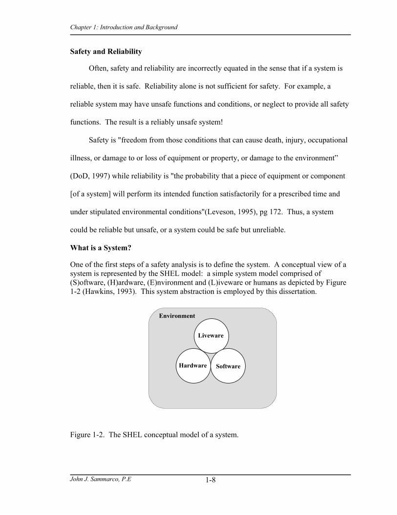
One of the first steps of a safety analysis is to define the system. A conceptual view of a system is represented by the SHEL model: a simple system model comprised of (S)oftware, (H)ardware, (E)nvironment and (L)iveware or humans as depicted by Figure 1-2 (Hawkins, 1993). This system abstraction is employed by this dissertation.
Figure 1-2. The SHEL conceptual model of a system.
Environment
Software
Liveware
Hardware

Chapter 1: Introduction and Background
John J. Sammarco, P.E
1-9
Safety must be from a system viewpoint. Safety cannot be assured if efforts are
focused only on part of the system because safety is an emergent property of the entire
system. Safety emerges once all subsystems have been integrated. For example, the
software can be totally free of “bugs” and employ numerous safety features, yet the
system can be unsafe because of how the software interacts and operates with the other
parts of the system. In other words, the sum may not be as safe as the individual parts.
The System Safety Approach
System safety, as defined by the military standard MIL-STD 882D, is "the
application of engineering and management principles, criteria and techniques to achieve
acceptable risk, within the constraints of operational effectiveness, time and cost
throughout all phases of the system life cycle" (DoD, 1997). System safety received
much scientific attention during and after World War II. This was the time when most of
our traditional safety techniques were developed to address new challenges posed by
systems that were more complex due to the use of new technology (Leveson, 1995). The
traditional "fly-fix-fly" approach to safety did not work well with these complex systems.
It was too dangerous, costly and wasteful to continue with this "after-the-fact approach",
so the system safety concept was initiated as a "before-the- fact" process (Roland &
Moriarity, 1982). The key concepts are listed:
1) Integrating safety into the design 2) Systematic hazard identification and analysis 3) Addressing the entire system in addition to the subsystems and components 4) Using qualitative and quantitative approaches
The system safety process is documented in MIL-STD-882, the most widely known
safety standard. Existing safety standards are built upon collections of expertise and
experiences (lessons learned) involving fatalities, injuries and near misses. In general,

Chapter 1: Introduction and Background
John J. Sammarco, P.E
1-10
standards also provide uniform, systematic approaches. History has shown that standards
are effective tools for safety (Leveson, 1992). Many safety standards have been created.
The Software Verification Centre of the University of Queensland in Australia has
compiled an international survey of safety standards (Wabenhorst & Atchison, 1999).
Hermann (Herrmann, 1999) presents detailed information concerning standards of key
industrial sectors.
Hazard Analysis
Hazard analysis is a key component of the system safety approach. A hazard is
"any real or potential condition that can cause injury, illness, or death to personnel or
damage to or loss of equipment or property, or damage to environment" (DoD, 1997).
Many techniques, ranging from simple qualitative methods to advanced
quantitative methods, are available to help identify and analyze hazards. The System
Safety Analysis Handbook (System Safety Society, 1997) provides extensive listings and
descriptions. Some examples of the more commonly used techniques are the Preliminary
Hazard List (PHL), Preliminary Hazard Analysis (PHA), Hazard and Operability Study
(HAZOP) and Failure Modes and Effects Analysis (FMEA). The use of multiple hazard
analysis techniques is recommended because each has its own purpose, strengths and
weaknesses. Typically, each technique addresses certain aspects of safety; thus, one
technique alone is not sufficient to identify and analyze all hazards of a system.
To be effective, the hazard analysis process must be applied over the life cycle of
the system in a continual and iterative manner. That is, hazard identification and analysis
must start at the conceptual stage of the system life cycle, when there are easier and less
costly to address. Hazard analysis continues on through the definition, development,
production, and deployment stages. The systematic approach to safety is captured in the

Chapter 1: Introduction and Background
John J. Sammarco, P.E
1-11
safety life cycle. It enables safety to be “designed in” early rather than being addressed
after the system’s design is completed.
The Safety Life Cycle
The use of a safety life cycle is required to ensure that safety is applied in a
systematic manner, thus reducing the potential for design errors. The safety life cycle
concept is applied during the entire life of the system. Hazards can become evident at
later stages or new hazards can be introduced by system modifications. Figure 1-3
depicts the safety life cycle phases (International Electrotechnical Commission (IEC),
1997).
The safety life cycle must be integrated within the overall product development life
cycle because safety issues impact overall development issues and vice versa. Secondly,
an integrated approach minimizes the likelihood of addressing safety as an afterthought
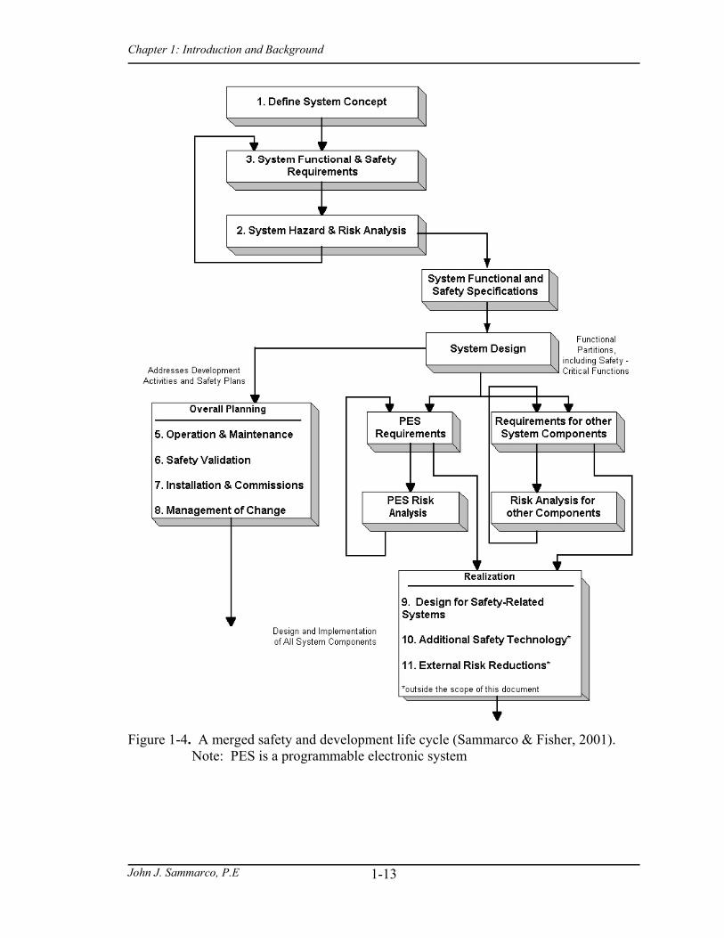
of the system design. An example merging the safety life cycle of Figure 1-3 with the
development life cycle is shown in Figure 1-4.

Chapter 1: Introduction and Background
John J. Sammarco, P.E
1-12
Figure 1-3. The safety life cycle (International Electrotechnical Commission, 1997).
Chapter 1: Introduction and Background
John J. Sammarco, P.E
1-13
Figure 1-4. A merged safety and development life cycle (Sammarco & Fisher, 2001).
Note: PES is a programmable electronic system

Chapter 1: Introduction and Background
John J. Sammarco, P.E
1-14
Faults, Errors, and Failures
There is confusion concerning faults, errors and failures; often the terms are used
interchangeably. Figure 1-5 depicts the relationship between a fault, error, and failure.
Figure 1-5. Fault, Error, and Failure Relationship.
A failure is "the termination of the ability of a functional unit to perform a required
function"(International Electrotechnical Commission (IEC), 1998). This definition is
based on a performance of a function, so failure is a behavior occurring at an instant in
time. A fault is an abnormal condition. Faults are random (hardware) or systematic
(hardware or software). Random faults are due to physical wear-out, degradation, or
defects; random faults can be accurately predicted and quantified. Systematic faults
concern the specification, design, and implementation. Software faults are systematic.
Faults, both random and systematic, may lead to errors (Storey, 1996).
An error is a system state that potentially can lead to a failure. When a fault results
in an error, the error is then a manifestation of the fault and the fault becomes apparent.
Not all faults lead to errors or failures. Some faults are benign or are tolerated such that
failure does not occur. Some faults are dormant such that an error state or failure does
not occur because the proper conditions do not exist. For example, a fault could reside in
a section of software. If that section of software is not used, then neither an error state
nor failure will occur.
FaultC ondition
M anifests as
(fault la tency)
Leads to
(error la tency)
E rrorS tate
F ailure

Chapter 1: Introduction and Background
John J. Sammarco, P.E
1-15
How Does Software Contribute to Complexity?
Software is especially prone to complexity because it can be non-deterministic,
contain numerous branches and interrupts, contain temporal criticality and consist of
hundreds of thousands of lines of code. Software does not exhibit random wear out
failures. Instead, software failures result from logic or design errors.
Beizer (Beizer, 1990) gives an example illustrating an aspect of software
complexity concerning the number of paths for a section of code. Given that a section of
software has 2 loops, 4 branches and 8 states, Beizer calculates the number of paths
through this code to exceed 8000!
Complexity and Safety
Simplification is one of the most important design aspects for safety. Complexity
makes it more difficult to conceptualize, understand, specify, design, test, document,
maintain, modify, and review the system. Complexity also makes it more likely for
errors, failure, and unplanned interactions to occur that may cause unsafe conditions. It
also increases demands on humans to operate and maintain the system. As a result,
humans can unknowingly put the system in an unsafe state during operation or
maintenance.
Definitions
Complexity: a) having many varied interrelated parts, patterns, or elements and consequently hard to understand fully; b) marked by an involvement of many parts, aspects, details, notions and necessitating earnest study or examination to understand or cope with (Gove, 1996).
Coupling: A measure of the strength of the interconnectedness between system components.

Chapter 1: Introduction and Background
John J. Sammarco, P.E
1-16
Error: A discrepancy between a computed, observed or measured value or condition and the true, specified or theoretically correct value or condition (International Electrotechnical Commission (IEC), 1998).
Failure: The termination of the ability of a functional unit to perform a required function (International Electrotechnical Commission (IEC), 1998).
Fault: An abnormal condition that may cause a reduction in, or loss of, the capability of a functional unit to perform a required function (International Electrotechnical Commission (IEC), 1998).
Hazard: Any real or potential condition that can cause injury, illness, or death to personnel or damage to or loss of equipment or property, or damage to environment (Reason, 1999).
Interactive complexity: Complex interactions are those of unfamiliar sequences, or unplanned and unexpected sequences and either not visible or immediately comprehensible (Perrow, 1999).
Measure: A mapping from a set of entities and attributes in the real world to a representation or model in the mathematical world (Fenton & Pfleeger, 1997).
Mistake (Human error): A human action or inaction that produces an unintended result (International Electrotechnical Commission (IEC), 1998).
Probabilistic risk assessment (PRA): A systematic method that includes risk analysis and the derivation of risk profiles in order to quantify the outcomes and their probability or likelihood (Kumamoto & Henley, 1996).
Reliability: Probability that failure time T is greater than operating time t ((Siewiorek, 1998).
R(t) = P(T>t) (1-1)
or
R(t) = e -8t (1-2)
for an exponential probability distribution
where 8 = failures / (time or natural units)
Risk: The combination of the probability of occurrence of harm and the severity of that harm (International Electrotechnical Commission (IEC), 1998).
Risk assessment: Assessment of the system or component to establish that the achieved risk level is lower than or equal to the tolerable risk level (Welch, 1998).
Chapter 1: Introduction and Background
John J. Sammarco, P.E
1-17
Safety: Freedom from those conditions that can cause death, injury, occupational illness, or damage to or loss of equipment or property, or damage to the environment (Reason, 1999).
Safety-critical: A term that describes any condition, event, operation, process or item of whose proper recognition, control, performance or tolerance is essential to safe system operation or use; e.g., safety-critical function, safety-critical path, safety-critical component (Reason, 1999).
Software Error: An incorrect step, process, or data definition; for example, an incorrect instruction in a computer program.
Software Failure: An event in which a system or system component does not perform a required function within specified limits (Welch, 1998).
Software Fault: A manifestation of an error in the software. If encountered, a failure might result (Welch, 1998).
Software Reliability: The probability that software will not cause the failure of a system for a specified time under specified conditions. The probability is a function of the inputs to and use of, the system as well as a function of the existence of faults in the software. The inputs to the system determine whether existing faults, if any, are encountered (Welch, 1998).
Subsystem: An element of the system that itself may be a system (Reason, 1999).
System: A collection of hardware, software, humans and machines interconnected to perform desired functions.
System accident: The unintended interaction of multiple failures in a tightly coupled system that allows cascading of the failures beyond the original failures (Perrow, 1999).
System reliability: The probability that a system, including all hardware and software subsystems, will perform a required task or mission for a specified time in a specified operational environment (Welch, 1998).
System safety: The application of engineering and management principles, criteria and techniques to achieve acceptable risk, within the constraints of operational effectiveness, time and cost throughout all phases of the system life cycle (Reason, 1999).
Summary
Escalating computer technology utilization is resulting in complex systems
containing new types of hazards having the potential to result in accidents. The
complexity of these systems makes it more likely for errors, failure and unplanned

Chapter 1: Introduction and Background
John J. Sammarco, P.E
1-18
interactions that can cause accidents. The generalized problem is that the nature of
accidents has changed for complex, computer-controlled systems; however, our
assessment methods have remained unchanged since their inception during World War II;
thus, another approach as needed. Our research is a first step to address this need by
developing a methodology to assess and quantify NAT complexity at the system level.
Finally, relevant background information was presented to provided a foundation of
basic safety concepts, clarify commonly misunderstood relationships, and introduce
terminology in order to provide a common understanding and enable effective
communication.
Literature Cited
Beizer, B. (1990). Software Testing Techniques. Second edition.
Davis, A. M. (1993). Software Requirements: Objects, Functions, and States. Prentice Hall.
DoD. (1997). (Report No. MIL-STD-882D). U.S. Department of Defense.
Fenton, N., & Pfleeger, S. L. (1997). Software Metrics: A Rigorous and Practical Approach. PWS Publishing Co.
Fiscor, S. (1998). U.S. Longwall Census. Vol. 3 (No. 2), pp. 22-27.
Gove, P. B. (Chief Editor). (1996). Webster Third New International Dictionary. Merrian Webster Inc.
Hawkins, F. H. (1993). Human Factors in Flight. Ashgate Publishing Company.
Herrmann, D. S. (1999). Software Safety and Reliability. IEEE Computer Society.
International Electrotechnical Commission (IEC). (1998). (Report No. IEC 61508-4). International Electrotechnical Commission.
International Electrotechnical Commission (IEC). (1997). (Report No. IEC 61508-7). International Electrotechnical Commission.
Kelly, J., Sherif, J., & Hops, J. (1992). An analysis of defect densities found during software inspections. Journal of Systems and Software, Vol. 17, pp. 111-117.

Chapter 1: Introduction and Background
John J. Sammarco, P.E
1-19
Kumamoto, H., & Henley, E. J. (1996). Probabilistic Risk Assessment for Engineers and Scientists. IEEE Press.
Ladkin, P. B. (1996). (Report No. RVS-RR-96-13). University of Bielefeld, Germany:
Leveson, N. G. (1986). Software Safety: Why, What, and How. ACM Computing Surveys, Vol. 18 (No. 2), pp. 125-163.
Leveson, N. G. (1992). High-pressure steam engines and computer software. International Conference on Software Engineering.
Leveson, N. G. (1995). Safeware: System Safety and Computers. Addison Wesley Publishing Co.
Leveson, N. G. (2000). System Safety in Computer-Controlled Automotive Systems. SAE Congress.
Littlewood, B., & Strigini, L. (1992). The Risks of Software. pp. 62-67.
Lutz, R. R. (1996). Targeting Safety-Related Errors During Software Requirements Analysis. The Journal of Systems Software, Vol. 34, pp. 223-230.
MacKenzie, D. (1994). Computer-Related Accidental Death: An Empirical Exploration. Science and Public Policy, Vol. 21, pp. 233-248.
Mellor, P. (1994). CAD: Computer-Aided Disaster. High Integrity Systems, Vol. 1(2), pp. 101-156.
Nelson, M., Clark, J., & Spurlock, M. A. (1999). Curing the Software Requirements and Cost Estimating Blues. pp. 54-60.
Neumann, P. G. (1995). Computer Related Risks The ACM Press.
Perrow, C. (1999). Normal Accidents: Living with High-Risk Technologies. Princeton, NJ: Princeton University Press.
Philips, M. M. (March 18, 1997). Business of mining gets a lot less basic. The Wall Street Journal.
Reason, J. (1999). Human Error. The Press Syndicate of the University of Cambridge.
Roland, H. E., & Moriarity, B. (1982). System Safety Engineering and Management. John Wiley & Sons.
Rushby, J. (1994). Critical System Properties: Survey and Taxonomy. Reliability Engineering and System Safety, Vol. 43(No. 2), pp. 189-219.
Sammarco, J. J. (2002). A Complexity Assessment Methodology for Programmable Electronic Mining Systems. The 20th International System Safety Conference.
Chapter 1: Introduction and Background
John J. Sammarco, P.E
1-20
Sammarco, J. J. (2003). Addressing the Safety of Programmable Electronic Mining Systems: Lessons Learned. 2002 IEEE Industry Applications Conference.
Sammarco, J. J., & Fisher, T. J. (2001). (Report No. IC 9458). NIOSH.
Siewiorek, D. P. S. R. S. (1998). Reliable Computer Systems: Design and Evaluation (3rd Ed.). AK Peters.
Storey, N. (1996). Safety-Critical Computer Systems. New York: Addison-Wesley Longman Inc.
System Safety Society. (1997). The System Safety Analysis Handbook. Section 3.0.
Wabenhorst, A., & Atchison, B. (1999). (Report No. Technical Report No. 99-30). Australia.
Welch, N. T. (1998). System Safety Analysis: A Human-Centric Approach. 16th International Systems Safety Conference, System Safety Society.
Wolf, F. G. (2000). Normal Accidents and Petroleum Refining: A Test of the Theory Unpublished doctoral dissertation, Nova Southeastern University.

Chapter 2: Research Objective and Specific Aims
John J. Sammarco, P.E 2-1
CHAPTER 2 RESEARCH OBJECTIVE AND SPECIFIC AIMS
Our ability to understand and manage the complexities of computer-based systems
has not kept pace with the technology=s utilization. We are ill-equipped because a
scientific methodology does not exist to identify and quantify the most important
attributes of complexity that impact the safety of these systems. As a result, computer-
related accidents causing mission failures, harm to the environment, injuries, and
fatalities have occurred. Neumann (Neumann, 1995) documented over 400 computer-
related accidents and MacKenzie determined that about 2000 deaths were computer-
related (MacKenzie, 1994).
Accidents resulting from system complexity are explained by Normal Accident
Theory (NAT). This theory has much support (Leveson, 2000; Mellor, 1994; Rushby,
1994; Sagan, 1993); however, only Wolf has operationalized NAT. His research (Wolf
2000) is specific to petroleum refining processes.
Our research is a first step that operationalizes NAT for the requirements phase. It
is a step that transfers theory to practice by establishing concrete, quantifiable
system-level complexity metrics so that complexities impacting safety can be identified
and reduced before they are propagated to other development phases. The ability to
quantify complexity is extremely important. As Lord Kelvin stated:
When you can measure what you are speaking about, and express it in numbers, you know something about it; but when you cannot measure it, when you cannot express it in numbers, your knowledge is of a meager and unsatisfactory kind: it may be the beginning of knowledge, but you have scarcely, in your thoughts, advanced it to the stage of understanding (William Thomson (Lord Kelvin), 1889).
Chapter 2: Research Objective and Specific Aims
John J. Sammarco, P.E 2-2
Research Objective
To develop a complexity assessment methodology for system requirements of safety-
related computer systems by operationalizing Normal Accident Theory (NAT).
Specific Aims
1. Identify the NAT attributes to operationalize with respect to system requirements.
2. Identify a formal modeling method for system requirements that will afford quantification of the potential metrics.
3. Identify potential metrics for each NAT attribute to be operationalized. At least one metric, and ideally four metrics, should be identified for each of these NAT attributes.
4. Determine which, if any of the potential metrics are useful measures or indicators of NAT complexity.
Literature Cited
Leveson, N. G. (2000). System Safety in Computer-Controlled Automotive Systems. SAE Congress.
MacKenzie, D. (1994). Computer-Related Accidental Death: An Empirical Exploration. Science and Public Policy, Vol. 21, pp. 233-248.
Mellor, P. (1994). CAD: Computer-Aided Disaster. High Integrity Systems, Vol. 1(2), pp. 101-156.
Neumann, P. G. (1995). Computer Related Risks. The ACM Press.
Rushby, J. (1994). Critical System Properties: Survey and Taxonomy. Reliability Engineering and System Safety, Vol. 43(No. 2), pp. 189-219.
Sagan, S. D. (1993). The Limits of Safety. Princeton University Press.
Thomson, W. (Lord Kelvin) (1889). The Sorting Demon of Maxwell. Collected in Popular Lectures and Addresses, vol. I, Constitution of Matter, Macmillan and Co, 1889.
Wolf, F. G. (2000). Normal Accidents and Petroleum Refining: A Test of the Theory. Unpublished doctoral dissertation, Nova Southeastern University.
Chapter 2: Research Objective and Specific Aims
John J. Sammarco, P.E 3-3
CHAPTER 3 LITERATURE REVIEW
This chapter discusses previous work in Normal Accident Theory (NAT) and
complexity metrics, critiques the limitations and inadequacies of this research, and draws
distinctions between prior work and the proposed research.
Normal Accident Theory
Perrow, an organizational theorist, is the originator of NAT. His work began in
1979 when he was advising a presidential commission investigating the accident at Three
Mile Island. Basically, Perrow identified system complexity as the primary accident
cause and identified system complexity attributes. A system accident, as defined by
Perrow, involves the unintended interaction of multiple failures in a tightly coupled
system that allows a cascading of failures. He concluded that these accident types were
built-in or inevitable with complex, high technological systems; Perrow stated these
accidents were a Anormal” occurrence because of complexity; hence, the theory was
named Normal Accident Theory. This theory identifies two important system
characteristics, tight coupling and interactive complexity, make complex software driven
systems especially prone to system accidents (Perrow, 1999). Tables 3-1 and 3-2,
respectively, list the system attributes for interactive complexity and tight coupling.
Interactively complex systems have the potential to generate many nonlinear branching
paths among subsystems. These interactions can be unexpected, unplanned,
incomprehensible, and unperceivable to system designers or system users. Therefore,

Chapter 3: Literature Review
John J. Sammarco, P.E
3-4
abnormal outcomes are more likely and human interventions are less likely to mitigate
the abnormal outcomes.
Coupling is a measure of the strength of the interconnectedness between system
components. Tightly coupled systems have little or no slack; thus, they rapidly respond
to and propagate perturbations such that operators do not have the time or ability to
determine what is wrong. As a result, human intervention is unlikely or improper.
Table 3-1. Tight Coupling Attributes Tight Coupling Attributes Comments Time-dependency Less tolerant of delays Sequences Invariant sequences Flexibility Equifinality or limited ways to reach the goal or
implement a function Slack Little or no slack in system structure or behavior Substitutions Limited substitutions of system components, units,
or subsystems. Table 3-2. Interactive Complexity Attributes Complex System Attributes Comments Proximity Close proximity of physical components or process
steps, less underutilized space Common-mode connections Many common-mode connections Interconnected subsystems Many interconnections Substitutions Limited substitutions of people, hardware, or
software; exacting requirements Feedback loops Unfamiliar or unintended feedback loops Control parameters Multiple and interacting control parameters Information quality Indirect, inferential, or incomplete information Understanding of system structure and behavior
Limited, incomplete, or incorrect understanding.
Normal Accident Theory Limitations
Perrow=s complexity theory has made inroads with notable computer science
researchers (Leveson, 1995; Ladkin, 1996) although it is based in organizational theory.
However, there are opportunities to refine and extend Perrow's work. These

Chapter 3: Literature Review
John J. Sammarco, P.E
3-5
opportunities address the needs for complexity quantification, consideration of multiple
perspectives, and rigorous scientific validation. Also, Perrow acknowledges that the
theory has not been extended to computer technology. He states, "The metaphor of an
accident residing in the complexity and coupling of the system itself, not in the failures of
its components has seeped into many areas where I never thought to apply it. I have
listed these in Figure A.1 . . .” (Perrow, 1999; pg 354). His figure lists software as a
neglected or new area to consider.
Quantification
Hopkins (Hopkins, 1999) cites Aill-defined concepts@ and Athe absence of criteria
for measuring complexity and coupling@ as significant limitations. Kates notes the same
limitations and stated, Athe absence of clear criteria for measuring complexity and
coupling makes his [Perrow’s] examples seem anecdotal, inconsistent, and subjective
(Kates, 1986). Quantitative measures of interactive complexity and coupling would
address these limitations and could serve to promote the theory.
Linear and complex systems
Perrow uses linear systems as a contrast to complex systems. The opposite of a
complex system is a simple system. Simplification is very important for eliminating or
reducing hazards. Leveson supports this by writing: "One of the most important aspects
of safe design is simplicity. A simple design tends to minimize the number of parts,
functional modes, and interfaces, and it has a small number of unknowns in terms of
interactions with the system and with system operation." (Leveson, 1995; pg 405).

Chapter 3: Literature Review
John J. Sammarco, P.E
3-6
Multiple perspectives
NAT does not address multiple projections (perspectives). Complexity is
multidimensional so, incorporating multiple projections could give added insight to the
complexity problem.
The perspectives of the system designers and users are important. For example,
consider a system with two operational modes, automatic and manual. The user switches
the system from the automatic mode to manual mode to clear "jammed" material from the
system. When placing the system back to automatic mode, the system resumes operation
from its prior state in automatic mode. As a result, the person is injured by rotating
system components. This is a system accident from the user's perspective because the
system=s actions were unexpected and unplanned. The actions did not fit the user=s
mental model of operation. The user expected and planned to have the system resume
from the last state in manual mode, not the last state in automatic mode. From the
designer's perspective, there was no fault of the system because it behaved exactly as it
was designed. The designer's perspective is that the problem was operator error.
Another perspective, possibly of management, is that the problem was human error, and
more and better training is needed.
Limited rigorous validation
Perrow validated his theory with a wide variety of illustrative examples from
chemical processing, aviation, marine transport, military defense systems, mining, and
space missions. Sagan validated the theory using case studies from nuclear weapon
systems. Wolf empirically validated the theory using a combination of quantitative and
qualitative techniques.

Chapter 3: Literature Review
John J. Sammarco, P.E
3-7
Sagan conducted research to validate NAT by using case studies derived from
nuclear weapon safety; the primary test case concerned the Cuban missile crisis of
October 1962. Sagan acknowledged that "the study of the commanding control of U.S.
nuclear weapons and potential of accidental nuclear war is a tough test for the NAT"
(Sagan, 1993 pg 49). "In short the study is a tough test for the Normal Accident Theory.
If the NAT does well here, it will be shown to be even stronger than previously
estimated" (Sagan, 1993; pg 51). Sagan concluded that there is strong support for NAT,
a view counter to his initial beliefs.
Wolf (Wolf, 2000) researched the validity and application of Perrow's theory to
petroleum refineries. These are high-risk technical systems having a high degree of
process control. Wolf defined a refinery system as a hierarchy of system units, links, and
nodes. Refinery complexity depends on the number of unit processes, links, and nodes.
Links are the systems pipes that carry raw material, byproducts, final product, and
wastes. Nodes are points of connection and interconnection between unit processes and
links. They are also the points for control and monitoring of parameters such as flow,
pressure, and temperature.
At the system level, refineries employ three types of manufacturing processes:
continuous, semi-continuous, and batch. At the unit level, up to 15 distinct processes and
a multitude of process technologies can exist.
Wolf's empirical validation utilized a hybrid of quantified and qualified measures
for a research sample of 36 petroleum refineries operating from 1992 to 1997. He created
a "refinery-specific" index of complexity based on refinery process knowledge. This

Chapter 3: Literature Review
John J. Sammarco, P.E
3-8
index served to quantify and estimate the interactive complexity for a refinery. The index
of complexity was calculated using the following formula (Wolf, 2000) pg. 65:
Ciplant = ( ) ( )Q Qij
j
m
i
n
i
n
j
m
ijkk
r
== = = =∏∏ ∏ ∏ ∏
=
11 1 1 1 (3-1)
where Ciplant = Refinery complexity n = Number of refinery unit processes m = Number of nodes at process i r = Number of parameters at node j Qijk = Number of possible states of parameter k at node j for process i Qij = Number of possible states of all parameters at node j for process i Ci = Number of possible states of all parameters of all nodes for process i
Ciplant is the index of complexity representing the maximum number of states in
which the system could exist. Thus Ciplant is an index of complexity useful for relative
ranking of refineries with respect to complexity.
The second component of Perrow's theory is coupling. Wolf classified coupling
based on a classification of the manufacturing process. Continuous processes are more
tightly coupled because they are generally invariant, time dependent, highly sequential,
and have little slack. Semi-continuous and batch processes are more flexible in terms of
timing and sequencing so they are classified as less tightly coupled.
Wolf's conclusions support the validity of Perrow's theory. Refineries
characterized by high complexity and tight coupling had more occurrences of accidental
releases of hazardous materials and more fires and explosions. However, two limitations
are evident in this research.

Chapter 3: Literature Review
John J. Sammarco, P.E
3-9
First, the work is specific to refineries. Thus the quantification measure, index of
complexity, is not generalized to other applications, thus limiting its utilization across
various application domains. Second, his work is limited to a narrow application domain.
Wolf validates Perrow’s theory for a special set of accidents encountered by refineries:
untoward releases of hazardous material, fires, and explosions. These are typically
encountered in the refinery sector, further illustrating the limitation of his highly
specialized research.
Sharit (Sharit, 2000), another researcher utilizing NAT, developed a risk modeling
framework incorporating NAT. The model is used to identify system risks, potential
human errors, and affords a better understanding of complex systems. Sharit modeled an
emergency health care system. We differ with Sharit's view of complexity.
He states "What determines a system's interactive complexity - and establishes
whether it is complex or linear - is the presence of a number of system features or
attributes" (Note: italics added for emphasis.) Sharit is referring to the interactive
complexity attributes listed in Table 3-1. His statement infers the quantity of system
features or attributes alone determines complexity; therefore, quantity determines
complexity and all features or attributes have an equal contribution. This view is
analogous to counting lines of code to determine complexity. Secondly, it infers that a
single number can characterize the multiple dimensions of complexity.
This research does not agree with these inferences and will address the following
questions. Do all attributes contribute equally to system complexity, and if not, which
attributes contribute the most to complexity? Secondly, this research quantifies
complexity in multiple dimensions.

Chapter 3: Literature Review
John J. Sammarco, P.E
3-10
Complexity Metrics
The use of software complexity measures began in the 1970's as a tool to address
rising costs of software development. Software maintenance costs were up to 80 percent
of software development costs. Complex software was recognized to be harder and
costlier to maintain. Today, research in software measurement continues to be quite
active. Software complexity measures have broadened their applicability to predict
testing costs, development time and effort, numbers of errors, and numerous quality
attributes. As the application scope has broadened, the number of complexity measures
has mushroomed; Zuse (Zuse, 1991) characterizes 98 complexity measures.
Ince (Ince, 1985) describes three categories of software complexity measures:
lexemical counts, graph theoretical, and system design structure. Adding the category of
integrated results in the four categories described as follows:
5. Lexemical counts: Count the key language entities such as keywords and operators.
6. Graph theoretical: Graph based control models of the system are created and key graphic characteristics such cyclomatic complexity are calculated.
7. System design structure: The structure is defined in terms of internal and external coupling of subsystems and modules. Internal coupling of modules is named cohesion or strength. Highly cohesive modules are desirable because behavior is localized. The external relationship among modules is called coupling. Loose coupling gives a high degree of isolation which minimizes the interdependency of modules.
8. Integrated: Integrated metrics synthesize existing metrics as a multi-metric composite.

Chapter 3: Literature Review
John J. Sammarco, P.E
3-11
Lexemical counts
The best known lexemical counts are Halstead's metrics, Table 3-3, and lines of
code (LOC). Halstead's metrics are based on the measurement of two parameters,
operators and operands, where:
n1 = number of unique or distinct operators N1 = total usage of all operators n2 = number of unique or distinct operands N2 = total usage of all operands.
Table 3-3. Halstead metrics. Metric Formula Program length N = N1 + N2 Program vocabulary N = n1 + n2 Volume V = N * (LOG2 n) Difficulty D = (n1/2) * (N2/n2) Effort E = D * V Weaknesses in Halstead's metric are listed (Beizer, 1990): 1. Halstead's metric depends on completed code. 2. The metric ignores nested loops. 3. Operators and operands are treated equally. 4. There is no differentiation of operator types (i.e. if-then-else is counted the same as
do-while even though, in general, loops are problematic).
LOC, as the name implies, is a count of the lines of code. This metric is fraught
with problems such as what constitutes a line for counting (i.e., are comment lines
counted?), programming language and style dependencies, and the erroneous notion that
size and complexity have a causal relationship.
Graph theoretical
McCabe's cyclomatic complexity metric (McCabe, 1976) is one of the best known
graph theoretical metrics. Cyclomatic complexity is a measure of the number of

Chapter 3: Literature Review
John J. Sammarco, P.E
3-12
independent control paths for a software program. As a general rule, if the complexity is
greater than 10, redesign should be considered. This metric is calculated as:
V (g) = e - n +2 (3-2) where: e = number of edges n = number of nodes If "n" disconnected graphs exist, the overall complexity is calculated by:
V(g)total = Vn
1∑ (g)n (3-3)
Cyclomatic complexity was extended by Vakil to examine and identify system
mode transition complexities for a commercial aircraft auto-flight system (Vakil, 2000).
He developed a “Hybrid Automation Representation” to model the mode transitions of an
auto-flight system. Cyclomatic complexity was used to analyze the mode transitions of
this complex system. Vakil found a correlation between mode transitions having high
cyclomatic complexity and the apparent complexity, as identified from the perspective of
pilots.
McCabe's metric is not devoid of weaknesses (Beizer, 1990) (Fenton & Pfleeger,
1997). First, it assumes a linear relationship of total complexity because the complexity
of each part is summed. This effectively underestimates complexity because complexity
increases nonlinearly (Beizer, 1990). It also has a weakness concerning compound
predicates. Treating a compound predicate as a single construct yields a lower
complexity number compared to separating it as series of constructs.
System design structure
Henry and Kafura's fan-in and fan-out metric and various coupling metrics are
based on design structure. Henry and Kafura's metric is based on the program dimension

Chapter 3: Literature Review
John J. Sammarco, P.E
3-13
of data flow where complexity is a function of fan-in and fan-out. The complexity is
calculated as follows:
Information flow complexity M = L (fan-in x fan-out) 2 (3-4) where: L = program length (McCabe's metric or LOC can be used) Fan-in = number of calls into a module plus the number of data structures retrieved by the module Fan-out = number of calls out of a module plus the number of data structures updated by the module
The results from this metric can be quite misleading. For instance, if either fan-in
or fan-out is zero, then the complexity calculation result is zero. Similarly, if a group of
simple modules has high reuse, fan-in and fan-out would be quite large; thus, the program
complexity calculation becomes quite high even though the overall program is simple.
Other problems with this metric are detailed in a study by Shepard (McDermid,
1990). As a result of this study, a hybrid metric was created to overcome numerous
problems with Henry and Kafura's original metric. The hybrid metric, called Shepperd
complexity is calculated as Shepperd complexity (M) = (fan-in x fan-out) 2.
However, the results from this metric can also be quite misleading. If either fan-in
or fan-out is zero, then the complexity calculation result is zero.
Coupling metrics
Coupling metrics measure the degree of connectivity between the parts of the
system. Coupling contributes to complexity thus low coupling is desirable to reduce the
likelihood of error propagation, facilitate comprehension, and reduce the likelihood that
changes in one part of the system do not affect the other parts of the system.
Chapter 3: Literature Review
John J. Sammarco, P.E
3-14
Myers views coupling as a measure of independence or modularity (Myers, 1974).
He defined six types of coupling and ordered them into a coupling scale. The scale, from
lowest to highest coupling, is data coupling (best), stamp coupling, control coupling,
external coupling, common coupling, and content coupling (worst).
Offutt et al. extended Myers work by quantifying coupling, increasing the scale
granularity from six levels to 12, and by measuring coupling in various configurations
(Offutt, Harrold, & Kolte, 1993). Coupling could be measured between pairs of modules,
from a key module to all other modules, and for the entire system. Secondly, they
addressed limitations of other metrics work by considering bi-directional coupling, and
by giving prescriptive definitions for each coupling level.
Although Offutt et al. have 12 levels of coupling, none of these the coupling
attributes of NAT. Secondly, the metrics work presented is for the subsystem of
software; thus, additional research is needed for system-level metrics addressing NAT.
Integrated complexity metrics
Integrated complexity metrics synthesize existing metrics into multi-metric
composites. Coskun (Coskun & Grabowski, 2001) addressed the challenges of modeling
and measuring complexity by using an integrated metrics approach. Coskun's research
targets embedded real-time systems for large-scale safety critical host systems. For these
systems, safety and reliability are obviously important.
Coskun's approach utilizes an interdisciplinary complexity model encompassing six
domains; from this complexity model, four types of complexity are measured. The
model utilizes the domains of mathematics, computer science, economics, psychology
and cognitive sciences, social science, and system science. For instance, the

Chapter 3: Literature Review
John J. Sammarco, P.E
3-15
mathematical domain includes Halstead's metric and McCabe's cyclomatic complexity;
the economic approach includes metrics of resource consumption; the social sciences
domain includes NAT.
The metrics from these domains have different views, objectives, and measures.
The multiple views afforded by the interdisciplinary approach are desirable because a
single view can not capture an entire problem space. The multiple objectives, and
associated measures to realize these objectives, are somewhat problematic given the
application to large-scale safety critical host systems where safety and reliability are very
important as stated by the authors. Specifically, some of the metrics don not apply to
safety or reliability; these metrics address quality and cost objectives.
Coskun’s research identifies four types of complexity: architectural/ structural
complexity, data processing/ reasoning/ functional complexity, user interface complexity,
and decision support/ explanation complexity. It is quite desirable to define and measure
multiple types of complexity because a single measure can not capture the notion of
complexity. The four complexity types are related to various software layers; hence,
Coskun's research does not address complexity at the system level. Software metrics
alone are not sufficient to address safety or reliability because these are emerging
properties of the system.
Complexity metric's limited success
Although there is a plethora of complexity measures, there have been limited
successes. McDermid (McDermid, 1990) confirms this stating:
Complexity is both a major problem and an enigma, as there are no easy and effective ways of measuring it. ... There has been a lot of work on software

Chapter 3: Literature Review
John J. Sammarco, P.E
3-16
complexity measures, but it is widely accepted that these are not adequate and in many cases are misleading...
There are numerous reasons for the limited success of metrics; some reasons
concern weaknesses that have been described in the previous sections. Others provide
more insight.
Fenton’s (Fenton, 1994) analysis of software measurement identifies a fundamental
flaw; most measurements lack a basis in measurement theory. T. Capers Jones (Jones &
Vouk, 1990) addresses inaccurate metrics. He cites the root cause of inaccurate metrics
as “the widespread tendency to use concepts without examining their validity.” Existing
metrics measure what we understand and what we are able to measure. Also, much
metric research has insufficient validation.
While these criticisms of complexity measures may be valid, there is a much
broader flaw: many complexity measures exist for the subsystem of software, but they do
not address the level of the entire system. Software does not have physical properties and
therefore by itself is not hazardous. Also, each subsystem can be quite simple, but the
interconnections among the software, hardware, and environment could result in a very
complex system. Hence, complexity must be addressed at the system level.
Summary
This literature review reinforces the validity of NAT but indicates the absence of
research for the safety-critical system domain and scientific rigor, and it points out the
limitations and inadequacies of metrics research.
A review of work by Perrow, Sagan, and Wolf confirmed the validity of NAT.
Perrow originated the theory and validated it with illustrative examples from chemical
manufacturing, aviation, marine transport, military defense systems, mining, and space

Chapter 3: Literature Review
John J. Sammarco, P.E
3-17
missions. His illustrative validation methodology is a weakness because it lacks the rigor
of scientific quantification. Sagan validated the theory using case studies of nuclear
weapon systems. Wolf's empirical research has the strongest scientific support; however,
this research is limited to the petroleum process industry domain, so the metrics do not
adequately transfer to the safety-critical systems domain. A significant weakness of
Wolf’s metrics concerns the coarse granularity of coupling metrics where the degree of
coupling is assigned based upon the total manufacturing process.
Finally, a review of the most common complexity metrics is given for the
following categories:
1. Leximical counts: Halstead’s metrics, LOC
2. Graph theoretical: McCabe’s cyclomatic complexity
3. System design structure: Henry and Kafura’s fan-in and fan-out, Shepperd complexity
4. Integrated metrics: Coskun’s interdisciplinary complexity
This review describes numerous problems with metrics that include measurement
ambiguities, potentially misleading results, lack of a measurement theory basis, and the
tendency to use concepts without validation. Additionally, these metrics do not directly
address interactive complexity and coupling in terms of NAT, and these metrics pertain
to the software subsystem; thus, they don't address the complexity of the system.
Literature Cited
Beizer, B. (1990). Software Testing Techniques. Second edition.
Coskun, E., & Grabowski, M. (2001). An interdisciplinary model of complexity in Embedded Intelligent Real-Time Systems. Information and Software Technology, Vol. 43, pp. 527-537.
Chapter 3: Literature Review
John J. Sammarco, P.E
3-18
Fenton, N., & Pfleeger, S. L. (1997). Software Metrics: A Rigorous and Practical Approach. PWS Publishing Co.
Fenton, N. E. (1994). Software Measurement: A Necessary Scientific Basis. IEEE Transactions on Software Engineering, Vol. 20(No. 3), pp. 199-206.
Hopkins, A. (1999). The Limits of Normal Accident Theory. Safety Science, Vol 32, pp 93-102.
Ince, D. C. (1985). The Influence of System Design Complexity Research on the Design of Module Interconnection Languages. SIGPLAN Notices, Vol. 20(No. 10), pp. 36-43.
Jones, W. D., & Vouk, M. A. (1990). Software Reliability Handbook: Chapter 11, Field Data Analysis. City University, London: Centre for Software Reliability.
Kates, R. (1986). Book Review: Normal Accident. Vol. 38 (No. 1), pp. 121-122.
Ladkin, P. B. (1996). (Report No. RVS-RR-96-13). University of Bielefeld, Germany:
Leveson, N. G. (1995). Safeware: System Safety and Computers. Addison Wesley Publishing Co.
McCabe, T. (1976). A Complexity Measure. IEEE Transactions on Software Engineering, 2(4), pp. 308-320.
McDermid, J. (1990). Issues in the Development of Safety-critical Systems. F. Redmill & T. Anderson. Safety-critical Systems: Current Issues, Techniques and standards. Chapman and Hall.
Myers, G. (1974). Reliable Software Through Composite Design. New York: Mason and Lipscomb Publishers.
Offutt, A. J., Harrold, M. J., & Kolte, P. (1993). A Software Metric System for Module Coupling. The Journal of Systems and Software, Vol. 20, pp. 295-308.
Perrow, C. (1999). Normal Accidents: Living with High-Risk Technologies. Princeton, NJ: Princeton University Press.
Sagan, S. D. (1993). The Limits of Safety. Princeton University Press.
Sharit, J. (2000). A Modeling Framework for Exposing Risk in Complex Systems. Risk Analysis, Vol. 20, No.4, pp. 469-482.
Vakil, S. S. Analysis of Complexity Evolution Management and Human Performance Issues in Commercial Aircraft Automation Systems. Unpublished doctoral dissertation, Massachusetts Institute of Technology, Massachusetts Institute of Technology.

Chapter 3: Literature Review
John J. Sammarco, P.E
3-19
Wolf, F. G. (2000). Normal Accidents and Petroleum Refining: A Test of the Theory. Unpublished doctoral dissertation, Nova Southeastern University.
Zuse, H. (1991). Software Complexity: Measures and Methods. New York.

Chapter 4: System Modeling
John J. Sammarco, P.E
4-1
CHAPTER 4 SYSTEM FUNCTIONAL REQUIREMENTS MODELING
The objective of this chapter is to select a method to model system functional
requirements for safety critical embedded systems such that the model abstraction
enables direct or indirect measurement of NAT complexity. A well-defined system
model is critical if meaningful metrics are to be developed.
Twelve criteria were established to help guide the selection of a modeling method.
The selected modeling method, named Software Cost Reduction (SCR), is described
along with its associated tool set.
System Models
A model is useful for abstracting a real-world entity or process so that only the
features or characteristics of interest are shown. Models are useful for understanding;
they can reduce complexities by removing extraneous aspects and can afford different
projections or viewpoints. This becomes especially useful for complex systems because
these systems are often multidimensional. A complex system can Alook@ different
depending on the dimension captured by the projection. For instance, viewpoints can
capture structural or behavioral aspects, or they can capture a user's perspective by
modeling human interactions with the system. There are numerous types of models;
some argue that there are too many modeling approaches. One reason for so many
models is that each has different strengths, weaknesses, and capabilities; different types
of models are needed to investigate different aspects of an entity or process.

Chapter 4: System Modeling
John J. Sammarco, P.E
4-2
In the context of this work, the system model needs to enable direct or indirect
measurement of the NAT attributes captured by the system requirements. Generally,
system requirements define Awhat@ the system does − the system’s behavior. Design
requirements and specifications define the Ahow@ − the system=s structure.
System behavioral requirements, also called functional or operational requirements,
specify the system inputs (stimuli), the system outputs (responses), and the behavioral
relationships between the inputs and outputs. Nonfunctional requirements impose
various resource, timing, and performance constraints.
Thus, a model must be constructed with a specific purpose or objective in mind.
Selecting a model suitable for one=s objectives can be a time-consuming task given the
plethora of modeling types, methods, and tools. To simplify the selection of a model for
our research, we limit the modeling to the system requirements phase and establish
criteria for modeling safety critical embedded systems.
Overview of Model Types, Methods, and Tools
Requirements models can be categorized by three types: natural language, semi-
formal, and formal (Loucopoulos & Karakostas, 1995). Natural language is very flexible
but it is very difficult to precisely define the system because of language ambiguities.
Semiformal models include diagrams and tables. These have fewer ambiguities and
interpretations. Formal methods are very exacting and have a rigorous mathematical
foundation.
A categorization of functional requirements modeling and analysis is depicted in
Figure 4-1 (Easterbrook, 2001) where the most well-known semiformal and formal
methods for functional requirements modeling.

Chapter 4: System Modeling
John J. Sammarco, P.E
4-3
F u n c t io n a l R e q u ir e m e n t s
S t r u c t u r e d A n a ly s i s
J S DJ a c k s o n S y s t e m D e v e lo p m e n t
S A D TS t r u c tu r e d A n a ly s i s a n d D e s ig n T e c h n o lo g y
S A /R TS t r u c tu r e d A n a ly s i s /R e a l T im e
S S A D MS t r u c tu r e d S y s t e m A n a ly s i sa n d D e s ig n M e th o d
S t a t e c h a r t s
E tc .
O b j e c t O r ie n t e d A n a ly s i s
O O AO b je c t O r i e n t e d A n a ly s i s
O O S EO b je c t O r i e n t e d S o f tw a r e E n g in e e r in g
O M TO b je c t M o d e l in g T e c h n o lo g y
U M LU n i f i e d M o d e l in g L a n g u a g e
O M LO p e n M o d e l in g L a n g u a g e
T O ST a x o n o m ic O b je c t S y s t e m
E tc .
F o r m a l M e t h o d s
R S M LR e q u i r e m e n t s S t a t eM a c h in e L a n g u a g e
S C RS o f tw a r e C o s t R e d u c t io n
S t a t e c h a r t s
V D MV ie n n a D e v e lo p m e n t M e th o d
E tc .
Figure 4-1. An overview of requirements modeling methods. Source: Adapted and
extended from Easterbrook, 2001.
Requirements Modeling Criteria
Models have different strengths, weaknesses, and purposes; different types of
models are needed to investigate different aspects of an entity or process (Easterbrook,
2001). Therefore, criteria are established for selecting a modeling method that is
consistent with the objectives and delimitations of this dissertation. The criteria guide the
selection of an appropriate modeling method and are not utilized as a means to determine
the optimal modeling method for the research.
Specific Criteria
• Abstraction Level: The model must be applicable to the level of the system not just the subsystem of software, because safety and complexity are emergent properties of the entire system.
• Availability: The modeling technique and associated tools should be widely available to researchers and practitioners.
• Learning Curve: It should be relatively easy to learn so that resources can focus on the research and not learning the method and tools.
• Life cycle phase: The modeling technique and associated tools must be applicable to the requirements phase.

Chapter 4: System Modeling
John J. Sammarco, P.E
4-4
• Projection: The projection needs to capture the end-user’s viewpoint in order to investigate the externally visible behavior of the system.
• Time: Often, safety-critical embedded systems are real-time, so the model should be able to incorporate timing constraints.
• Real-world applicability: The model should be of Aindustrial@ strength so that it can handle the complexity and size of real-world problems as evidenced by a history of real-world utilization.
• Safety: Undesirable or unexpected system behavior can create a hazard. This type of behavior can occur during normal system operation or abnormal conditions. System accidents can occur when the end-user improperly responds to or fails to respond to normal or abnormal conditions. Therefore, the model must be able to model behavior for normal and abnormal conditions.
• Simulation: Capabilities should exist to interactively execute the specification. This interaction should be available to the model developer for analysis purposes, and to enable human interaction with the system.
• System Type: The model must be applicable to safety-critical embedded systems. Often, these systems are reactive, so the model must capture the system=s behavior to external stimuli from the environment and liveware.
• Tools: The model should have tools, preferably computer-based, to support the creation, modification and analysis of the model.
• User-interface support: The model=s tools should support extensions for a graphical user-interface to enable end-user interaction with the system.
Of the methods depicted by Figure 4-1, only unified modeling language (UML) and
SCR were able to meet most of these criteria. UML is a well-known language for object-
oriented analysis and design. UML was not selected because it did not meet the “learning
curve” criterion concerning the ease of learning. As whole, UML is complex. The UML
1.3 specification has over 800 pages and UML has numerous modeling diagrams:
• Use case diagrams • Class diagrams • Sequence diagrams • Component diagrams • Statechart diagrams • Collaboration diagrams

Chapter 4: System Modeling
John J. Sammarco, P.E
4-5
UML also has several limitations (Glinz, 2000) concerning use case diagrams.
These diagrams are used in the early requirements stages to describe how the system
interacts with the external actors. Lastly, UML does have commercially available tools;
however, these tools are not free as is the SCR set of tools. Although UML has several
limitations, this does not infer that UML is unsuitable to model system requirements; all
modeling languages have some limitations. UML models have been successfully used to
analyze software quality and architectural risks (Yacoub, Ammar, & Mili, 2000).
The SCR method was chosen because of the Navel Research Laboratory’s (NRL)
interest in this research and their willingness to give access to SCR knowledge,
experience, and SCR tools at no cost.
Software Cost Reduction (SCR) for Requirements
SCR was originally used for documenting and specifying the functional
requirements of the A-7-E aircraft's Operational Flight Program (Queins et al., 2000).
SCR is a powerful method for the formal specification, analysis, and validation of
complex, embedded systems for a variety of systems including telephone networks,
avionics, safety-critical control systems for nuclear power plants, and the International
Space Station. During the mid 1990's, SCR was extended from software requirements to
system requirements; these extensions included the incorporation of nonfunctional
requirements such as timing and accuracy constraints. Additionally, NRL developed
support for integrated tools called the SCR* tool set.
The SCR method formalizes functional behavior as mathematical relations. These
relations are part of the Parnas Four-Variable Model. This is a model of requirements
that is essentially a black box view of system inputs, outputs, and external behavior; thus,

Chapter 4: System Modeling
John J. Sammarco, P.E
4-6
the model captures the required external behavior, devoid of implementation or structural
aspects of the design. SCR also employs tables with a relatively simple formal notation
to define mathematical functions; hence, SCR tables facilitate industry utilization because
the tables and the notation are easily created and understood (Heninger, Parnas, Shore, &
Kallander, 1978).
SCR Four-Variable Model
The Four-Variable Model partitions a system into four elements: the environment,
input devices, software, and output devices. The model's projection captures
synchronous behavior, as viewed externally, and hardware/software interfaces to the
environment. The external behavior is from the perspective of the user, although the
model does not explicitly depict the user as part of the system as in the SHEL model.
Because, in the context of this work, complexities are from the user's perspective, we
extend the Parnas Four-Variable Model to include the liveware element of the SHEL
model. This model extension is depicted by Figure 4-2.
Figure 4-2. The SCR Four-Variable Model extended to incorporate the SHEL model

Chapter 4: System Modeling
John J. Sammarco, P.E
4-7
The required behavior is formalized by the Four-Variable Model as follows (Heninger et
al., 1978):
The Four-Variable Model . . . describes the required system behavior, including
the required timing and accuracy, as a set of mathematical relations on four sets of
variablesCmonitored and controlled variables and input and output data items. A
monitored variable represents an environmental quantity that influences system
behavior, a controlled variable [is] an environmental quantity that the system
controls. A black-box specification of required behavior is given as two relations,
REQ and NAT, from the monitored to the controlled quantities. NAT, which
defines the set of possible values, describes the natural constraints on the
system behavior, such as constraints imposed by physical laws and the
system environment. REQ defines additional constraints on the system to
be built as relations the system must maintain between the monitored and
the controlled quantities.
In the Four-Variable Model, input devices (e.g., sensors) measure the
monitored quantities and output devices set the controlled quantities;
input and output data items represent the values that the devices read and
write.
SCR represents monitored and controlled quantities as variables. The dependent
variables are the controlled variables, mode classes, and terms; the independent variable
is the monitored variable.
To summarize the flow through the Four-Variable Model, monitored and controlled
quantities are within the environment=s domain; input devices transform monitored
quantities to input data that are represented by SCR models as monitored variables;
output devices transform output data, represented by SCR models as controlled variables,
such that the controlled quantities are manipulated.

Chapter 4: System Modeling
John J. Sammarco, P.E
4-8
The system's behavioral requirements are defined by the NAT and REQ relations
for ideal behavior. These relations can be extended to non-ideal behavior encountered in
the real world. Non-ideal behavior specifies the response to undesired events. Sources
for non-ideal behavior include hardware malfunctions or incorrect human interactions
with the system. The non-ideal behavior combined with the ideal behavior is defined by
the NAT relation.
SCR Terminology and Notation
The basic concepts of SCR have been presented. SCR terminology and notation
(Heitmeyer, 1996) is presented in order to establish a common understanding of SCR
specifications.
Condition: A condition c is a logical expression for an input or output variable, mode, or term. Conditions may be simple or compound.
Condition Table: This table defines a given controlled variable or term as a function of the possible modes and associated conditions for each mode. Thus, it defines the value of controlled variables or terms for all conditions.
Event: An event e is an instance in time when a mode, term, or variable changes value. For instance, an input event occurs when a monitored quantity changes; an output event occurs when a controlled quantity changes.
e = @T(c); a basic event where condition c changes to true e = @F(c) = @T(¬c); a basic event where condition c changes to false e = @T(c) WHEN d = a v aN; an event where a = next state, aN = old state Event Table: This table defines a given controlled variable or term as a function of the possible modes and associated events for each mode. Thus, it defines the response of controlled variables or terms to input events.
Mode: A state of the environment as represented by monitored variables.
Mode Class: A type of deterministic synchronous finite state machine comprised of modes that partition the state of the environment. Complex systems have multiple mode classes operating in parallel.
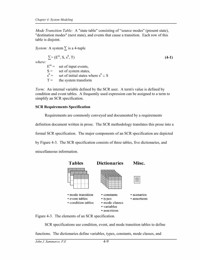
Chapter 4: System Modeling
John J. Sammarco, P.E
4-9
Mode Transition Table: A "state table" consisting of “source modes" (present state), "destination modes" (next state), and events that cause a transition. Each row of this table is disjoint.
System: A system 3 is a 4-tuple 3= (Em, S, s0, T) (4-1) where: Em = set of input events, S = set of system states, s0 = set of initial states where s0 f S T = the system transform Term: An internal variable defined by the SCR user. A term's value is defined by condition and event tables. A frequently used expression can be assigned to a term to simplify an SCR specification.
SCR Requirements Specification
Requirements are commonly conveyed and documented by a requirements
definition document written in prose. The SCR methodology translates this prose into a
formal SCR specification. The major components of an SCR specification are depicted
by Figure 4-3. The SCR specification consists of three tables, five dictionaries, and
miscellaneous information.
Figure 4-3. The elements of an SCR specification.
SCR specifications use condition, event, and mode transition tables to define
functions. The dictionaries define variables, types, constants, mode classes, and
Chapter 4: System Modeling
John J. Sammarco, P.E
4-10
assertions. Scenarios are composed of input event sequences and are used for simulation
purposes. Assertions define properties that must hold for the system. Typically, these
are safety and security properties.
Time and performance constraints can be incorporated into the SCR specification
(Heitmeyer, 1996). Time is represented by a monitored variable and is a non-negative
integer initialized to zero.
SCR*toolset
The NRL created the SCR*toolset (Maurer, 2000) to support the SCR
methodology. The tool set is an integrated suite of CASE tools publicly available from
NRL. The tool set has found relatively widespread use; it has been installed at over 100
organizations in industry, government, and academia, according to Heitmeyer (personal
communication, 2000).
The components of the SCR*toolset are shown in figure 4-4. This figure also
depicts the basic process of using the tool set to translate a requirements specification to
an SCR specification, analyze the specification, and validate the external behavior by
simulation.
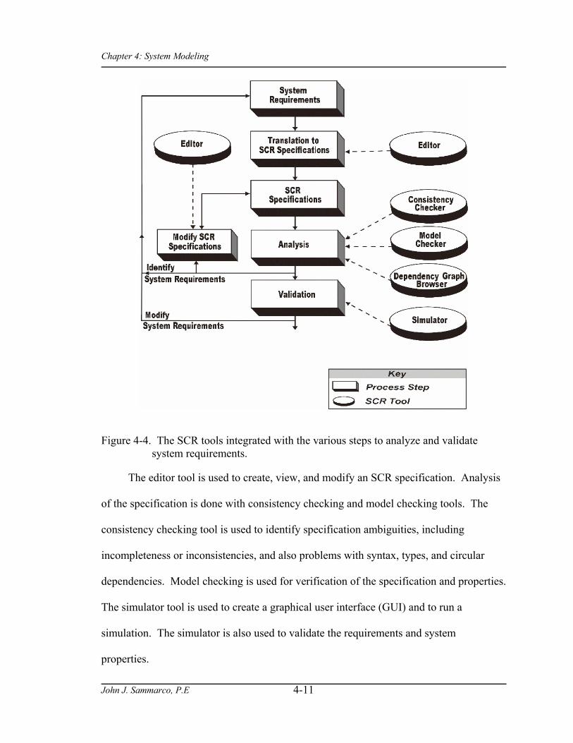
Chapter 4: System Modeling
John J. Sammarco, P.E
4-11
Figure 4-4. The SCR tools integrated with the various steps to analyze and validate system requirements.
The editor tool is used to create, view, and modify an SCR specification. Analysis
of the specification is done with consistency checking and model checking tools. The
consistency checking tool is used to identify specification ambiguities, including
incompleteness or inconsistencies, and also problems with syntax, types, and circular
dependencies. Model checking is used for verification of the specification and properties.
The simulator tool is used to create a graphical user interface (GUI) and to run a
simulation. The simulator is also used to validate the requirements and system
properties.

Chapter 4: System Modeling
John J. Sammarco, P.E
4-12
A second type of analysis is possible by utilizing SCR visualization tools. The
dependency graph browser, Figure 4-5, displays the dependencies between SCR model
variables (the controlled and monitored variables, modes, and terms) and gives a
graphical overview of the specification. It also provides a mapping of controlled
variables to monitored variables. The graph depicts each SCR variable as a node; a
dependency between nodes is represented by an arrow where the variable’s value at the
tail depends on its value at the head of the arrow.
A second graph is called the mode transition graph which is much like a state
transition diagram. A mode transition graph exists for each mode class.
The vertices or nodes represent modes and the directed arcs represent transitions.
Figure 4-6 shows an example mode transition graph, comprised of the modes (states)
Low, Normal, Voter Failure, for a mode class named M_Pressure.
Term s or M odesM onitored Variables
Controlled Variables
Figure 4-5. An SCR dependency graph. Source: Navel Research Laboratories

Chapter 4: System Modeling
John J. Sammarco, P.E
4-13
Figure 4-6. A mode transition graph for the mode class “M_Pressure” Source: Navel Research Laboratories
Summary
One of the first steps in the measurement process is to define the object or process
to be measured. Next, a systematic method is needed to determine what needs to be
measured and what abstraction or model can enable measurements. This chapter
established 12 criteria to help guide the selection of a modeling method. Based on these
criteria, the SCR method was selected. SCR and the supporting set of tools were
described in detail.
Literature Cited
Easterbrook, S. (2001) Lecture 8: Modeling Functional Behaviour [Web Page]. URL http://www.cs.toronto.edu/~sme/CSC2106S/index.html [2001, July 18].
Glinz, M. (2000) Problems and Deficiencies of UML as a Requirements Specification Language. Proceedings, 10th International Workshop on Software Specification and Design. November 11-22, 2000, San Diego, CA.

Chapter 4: System Modeling
John J. Sammarco, P.E
4-14
Heitmeyer, C. (1996). Requirements Specifications for Hybrid Systems. Proceedings, Hybrid Systems Workshop III, Lecture Notes in Computer Science Springer-Verlag.
Heninger, H., Parnas, D. L., Shore, J. E., & Kallander, J. W. (1978). (Report No. Technical Report 3876). Washington, DC: Navel Research Laboratory.
Loucopoulos, P., & Karakostas, V. (1995). System Requirements Engineering. McGraw Hill.
Maurer, H. (Ed.). (2000). Journal of Universal Computer Science (Vol. 6, No. 7). Springer Publishing Company.
Queins, S., Zimmerman, G., Becker, M., Kronengurg, M., Peper, C., Merz, R., & Schafer, J. (2000). The Light Control Case Study: Problem Description. Journal of Universal Computer Science; Special Issue on Requirements Engineering, Vol. 6, No. 7
Yacoub, Sherif M., Ammar, H., & Mili, A. (2000). A UML Model for Analyzing Software Qualtiy. Proceedings, International Conference on Reliability and Quality in Design. October 2000, Orlando, FL.

Chapter 5: Complexity Metrics
John J. Sammarco, P.E. 5-1
CHAPTER 5 COMPLEXITY METRICS
A graph-theoretical approach was used to operationalize NAT. Our objective was
to define multiple, graph-theoretical metrics to measure or indicate specific NAT
attributes of a system. The specific NAT attributes to operationalize are identified by a
three-step, systematic process.
Our approach also addresses the limitations of NAT and of other metric research,
described in the literature review of Chapter 3, by using multiple system abstractions and
perspectives to obtain metrics that can be precisely defined and quantified. Three levels
of system abstraction and three projections are used capture the multidimensional aspects
of complexity.
As a result, fifteen graph-theoretical metrics are proposed as measures or indicators
of specific NAT attributes of complex systems.
Graph Theory
Background information on graph theory is presented to establish terms and
definitions. Graph theory is useful for modeling and analyzing a variety of empirical
systems such as electrical circuits, communication networks, and transportation
scheduling networks. Graphs depict connections and relationships between a system’s
elements and subsystems thus enabling quantification of a system’s logic structure.

Chapter 5: Complexity Metrics
John J. Sammarco, P.E. 5-2
A large body of knowledge exists for graph theory. It has been studied since the
18th century; thus, the precise definitions, theorems, and axioms of graph theory are very
useful for this research.
Background information on graph theory is presented just to establish a common
understanding of terms and definitions. Next, examples are given showing how each
metric was calculated from SCR dependency graphs and SCR state information.
The SCR Dependency Graph
The SCR dependency graph represents mathematical relations as defined by the
SCR specification. The dependency graph, represented as G = (V, E), satisfies the
following:
• V(G): a finite, non-empty set of vertices. • E(G): a finite set of ordered pairs (u,v)of vertices called edges or directed edges. • For E(G), no two directed edges are parallel. • For E(G), a self loop is an edge e = (u,u) starting and ending at vertex u. Definitions:
Ancestors: The set of all ancestors anc(u) = {u ∈ U: there exists (u, v) ∈ E}.
Cyclomatic complexity: also known as the nullity of a graph. The number of linearly independent paths;
V (g) = e - n +2 (5-1) where: e = number of edges n = number of nodes If "n" disconnected graphs exist, the overall complexity is calculated by:
V (g) total = Vn
1∑ (g) n (5-2)
Descendent: The set of all descendents dep(u) = {v ∈ V: there exists (u, v) ∈ E}.
Direct ancestor: For (u,v), u is a direct ancestor of v.
Direct descendent: For (u,v), v is a successor or direct descendent of u.

Chapter 5: Complexity Metrics
John J. Sammarco, P.E. 5-3
Direct edge: An edge is represented by an arrow with a starting and ending point. A directed edge e = (u,v) starts at vertex u and ends at vertex v.
Graph degree: The sum of the in-degree and out-degree for a graph.
In-degree: The number of edges ending at a vertex. The in-degree id(u) of a vertex u is the number of edges (v, u) for all v ∈ V (G). In-degree is also known as fan-in.
Independent path: A linearly independent path contains at least one new vertex or edge.
Input vertex: If id(v) = 0, then v is an source or input
Local degree: The local degree of a vertex is the sum of the in-degree and the out-degree.
Out-degree: The number of edges starting at a vertex. The out-degree od(v) of a vertex v is the number of edges (u, v) for all v ∈ V (G). Out-degree is also known as fan-out.
Output vertex: If od(v) = 0, then v is an destination or output. Scenario subgraph: A subgraph S induced by the set of vertices involved by a scenario as simulated by the SCR simulator.
Self loop: An edge e = (u,u) starting and ending at vertex u.
Shepard complexity (M) = (id(v) x od(v))2.
Strict semipath: A joining of vertex v1, to vertex vn such that they are not mutually reachable. For example, in Figure 5-1, a strict semipath joins v1 and v3.
Figure 5-1. The vertices v1 and v3 are not mutually reachable because a strict semipath joins them.
Subgraph: A graph S whose vertices and edges are vertexes and edges of a graph G. The subgraph S is induced by a set of vertices of graph G.
Vertex: A vertex v is represented as a rectangle in a SCR dependency diagram.
Specific Attributes of Normal Accident Theory (NAT)
We revisited NAT with the objective of defining multiple, graph-theoretical metrics
to measure or indicate specific NAT attributes of a complex system. Specific NAT the

Chapter 5: Complexity Metrics
John J. Sammarco, P.E. 5-4
attributes to operationalize are identified by a process of deduction: 1) abstracting
Perrow’s thirteen attributes of complexity to a generalized view of simple (linear) and
complex (nonlinear) systems; 2) selecting a subset of NAT attributes pertaining to linear
and nonlinear systems; 3) identifying a general set of metrics to measure or indicate the
subset of NAT attributes.
First, the definition of complexity is established. Webster's dictionary defines
complexity as follows:
Complexity: (a) having many varied interrelated parts, patterns, or elements and consequently hard to understand fully; (b) marked by and involvement of many parts, aspects, details, notions, and necessitating earnest study or examination to understand or cope with (Gove, 1996).
This definition supports the structural and psychological aspects of NAT
complexity. Part (a) addresses the structural components of interconnections and
coupling; part (b) concerns the psychological component of comprehension and
confusion. Our primary interest is in the structural aspects of complexity evident in SCR
dependency graphs. Next, we review NAT attributes.
Perrow lists these thirteen attributes of complex systems (Perrow, 1999):
• close proximity • common-mode connections • many interconnections • limited substitutions • many feedback loops • poor information quality • limited or incorrect comprehension
• strict time-dependencies • invariant sequences • inflexible • limited slack • limited substitutions • interacting control parameters
Perrow also draws a major distinction between simple and complex systems:
simple systems are linear; nonlinear systems are complex.

Chapter 5: Complexity Metrics
John J. Sammarco, P.E. 5-5
Linear and Nonlinear Systems
Simple systems are linear; they do not have multiple branching paths
interconnecting system components and subsystems. A linear path is physically and
logically separated from other system parts; so, the path follows a predictable, sequential
order. A linear system is given involving a single line of dominos. A single disturbance
of a domino starts a linear chain of events where one domino pushes over the next. This
chain of events follows a highly observable, predictable, and linear sequence.
Nonlinear systems are complex because they are highly interconnected and
interactive. A single input or failure can generate many nonlinear branching paths
between system components and subsystems. These interactions can be unexpected,
unplanned, and incomprehensible to system users. A nonlinear system example is given
involving a car windshield. A single disturbance, such as a stone hitting the windshield,
causes a multitude of nonlinear, interconnected cracks. The chain of events from a single
stone, with respect to the cracks, is highly unpredictable and nonlinear because the stone
does not create a single, isolated crack.
A subset of NAT attributes
We used the high-level NAT abstraction of linear and nonlinear systems to focus
the scope of the problem of operationalizing NAT. As stated earlier, we are interested in
the structural aspects of complexity. Linearity is a structural aspect of system; therefore,
we determine a subset of Perrow’s thirteen NAT attributes pertaining to linearity. More
specifically, we select the NAT attributes present in SCR dependency graphs.

Chapter 5: Complexity Metrics
John J. Sammarco, P.E. 5-6
The resulting NAT attributes for linearity are as follows:
• Interconnectivity
• Common-mode connections
• Multiple, interacting control parameters
NAT attribute metrics
The third step of our process was to identify multiple metrics to measure or indicate
the specific NAT attributes of interconnectivity, common-mode connections, and
multiple, interactive control parameters.
We used graph theory to formally define metrics for interconnectivity. Figure 5-2
depicts a simple linear system. The linearity of this system can be quantified by
measuring the interconnectivity between vertices. In this example, the interconnectivity
is established by the path v1, v2, v3, and v4. More formally, the cyclomatic complexity
metric V (g) is indicative of the system’s interconnectivity. V (g) quantifies the number
of linearly independent paths where, for Figure 5-2, V (g) = 1.
Figure 5-2. A simple linear system with one linear path v1, v2, v3, and v4.
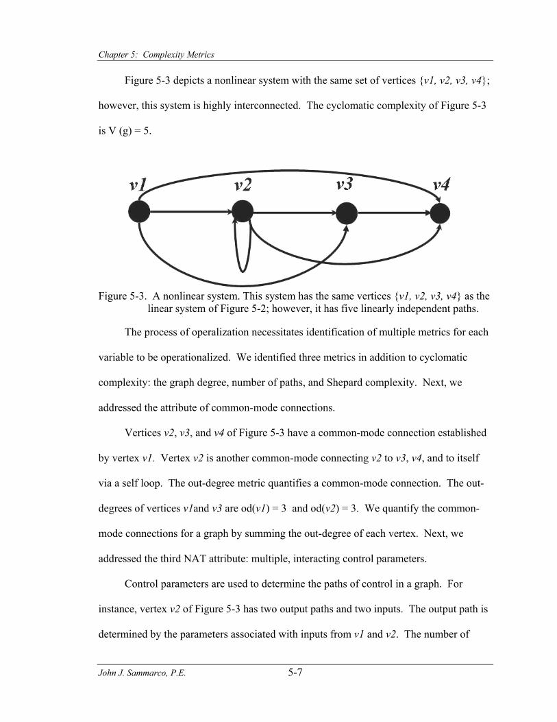
Chapter 5: Complexity Metrics
John J. Sammarco, P.E. 5-7
Figure 5-3 depicts a nonlinear system with the same set of vertices {v1, v2, v3, v4};
however, this system is highly interconnected. The cyclomatic complexity of Figure 5-3
is V (g) = 5.
Figure 5-3. A nonlinear system. This system has the same vertices {v1, v2, v3, v4} as the
linear system of Figure 5-2; however, it has five linearly independent paths.
The process of operalization necessitates identification of multiple metrics for each
variable to be operationalized. We identified three metrics in addition to cyclomatic
complexity: the graph degree, number of paths, and Shepard complexity. Next, we
addressed the attribute of common-mode connections.
Vertices v2, v3, and v4 of Figure 5-3 have a common-mode connection established
by vertex v1. Vertex v2 is another common-mode connecting v2 to v3, v4, and to itself
via a self loop. The out-degree metric quantifies a common-mode connection. The out-
degrees of vertices v1and v3 are od(v1) = 3 and od(v2) = 3. We quantify the common-
mode connections for a graph by summing the out-degree of each vertex. Next, we
addressed the third NAT attribute: multiple, interacting control parameters.
Control parameters are used to determine the paths of control in a graph. For
instance, vertex v2 of Figure 5-3 has two output paths and two inputs. The output path is
determined by the parameters associated with inputs from v1 and v2. The number of
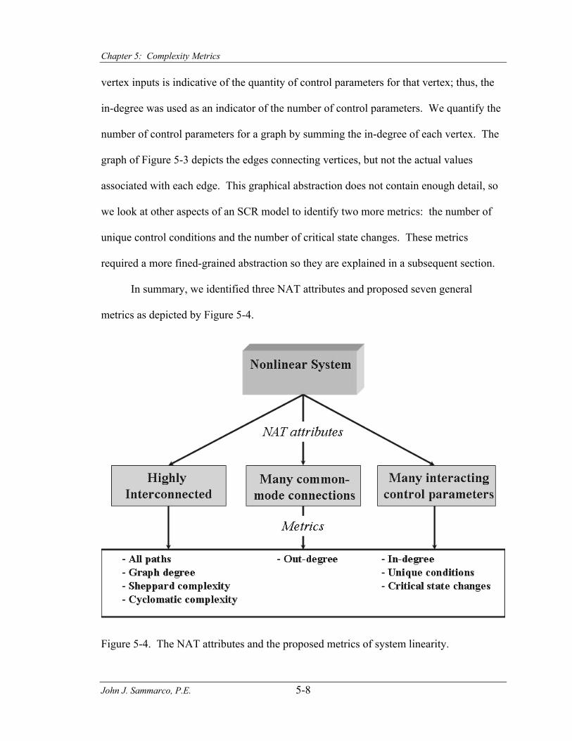
Chapter 5: Complexity Metrics
John J. Sammarco, P.E. 5-8
vertex inputs is indicative of the quantity of control parameters for that vertex; thus, the
in-degree was used as an indicator of the number of control parameters. We quantify the
number of control parameters for a graph by summing the in-degree of each vertex. The
graph of Figure 5-3 depicts the edges connecting vertices, but not the actual values
associated with each edge. This graphical abstraction does not contain enough detail, so
we look at other aspects of an SCR model to identify two more metrics: the number of
unique control conditions and the number of critical state changes. These metrics
required a more fined-grained abstraction so they are explained in a subsequent section.
In summary, we identified three NAT attributes and proposed seven general
metrics as depicted by Figure 5-4.
Figure 5-4. The NAT attributes and the proposed metrics of system linearity.

Chapter 5: Complexity Metrics
John J. Sammarco, P.E. 5-9
Metric Descriptions
Our approach to operationalize NAT addressed limitations of NAT and other
metric research as described in the literature review of chapter 3 by using:
• multiple metrics to quantify each NAT attribute
• three system abstractions for the metrics.
• three projections for each system abstraction
Three system abstractions
Three system abstractions were used in the process of determining metrics for NAT
attributes. The rational was that it was unlikely a single abstraction would contain all the
metrics because complexity is a multi-dimensional. Therefore, multiple abstractions
were needed. The following abstractions were created:
• the scenario subgraph, a course-grained abstraction; • the critical-state subgraph, a medium-grained abstraction; • the critical-vertex subgraph; a fine-grained abstraction. Scenario subgraph abstraction
The first level of abstraction is named the scenario subgraph. This course-grained
abstraction of an SCR dependency graph was defined by the subgraph induced by the
edges and vertices used during a scenario; therefore, unused edges and vertices are
eliminated. For example, Figure 5-5 depicts an SCR dependency graph of a system. The
highlighted (darkened) vertices are those used during a given scenario. Figure 5-6
depicts the resulting scenario subgraph of only the vertices and edges used for a given
scenario.
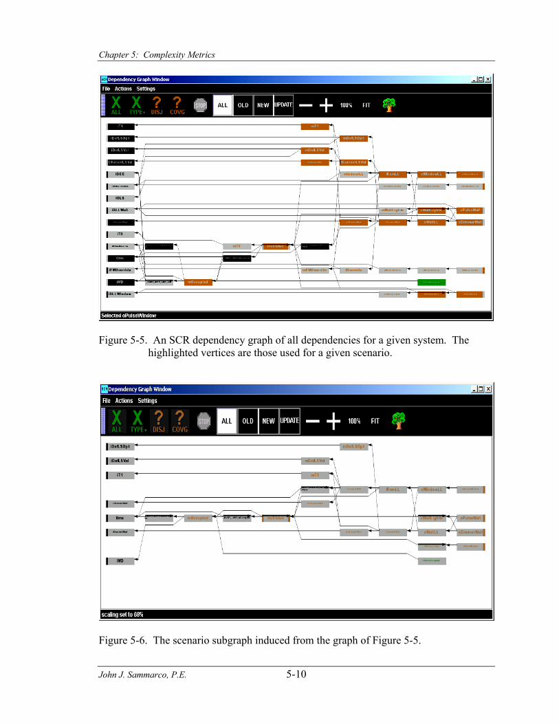
Chapter 5: Complexity Metrics
John J. Sammarco, P.E. 5-10
Figure 5-5. An SCR dependency graph of all dependencies for a given system. The
highlighted vertices are those used for a given scenario.
Figure 5-6. The scenario subgraph induced from the graph of Figure 5-5.
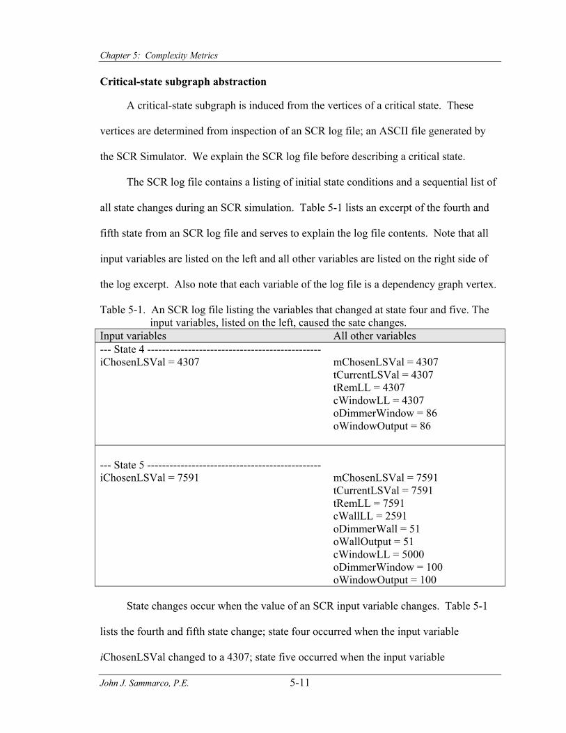
Chapter 5: Complexity Metrics
John J. Sammarco, P.E. 5-11
Critical-state subgraph abstraction
A critical-state subgraph is induced from the vertices of a critical state. These
vertices are determined from inspection of an SCR log file; an ASCII file generated by
the SCR Simulator. We explain the SCR log file before describing a critical state.
The SCR log file contains a listing of initial state conditions and a sequential list of
all state changes during an SCR simulation. Table 5-1 lists an excerpt of the fourth and
fifth state from an SCR log file and serves to explain the log file contents. Note that all
input variables are listed on the left and all other variables are listed on the right side of
the log excerpt. Also note that each variable of the log file is a dependency graph vertex.
Table 5-1. An SCR log file listing the variables that changed at state four and five. The input variables, listed on the left, caused the sate changes.
Input variables All other variables --- State 4 ----------------------------------------------- iChosenLSVal = 4307 mChosenLSVal = 4307 tCurrentLSVal = 4307 tRemLL = 4307 cWindowLL = 4307 oDimmerWindow = 86 oWindowOutput = 86 --- State 5 ----------------------------------------------- iChosenLSVal = 7591 mChosenLSVal = 7591 tCurrentLSVal = 7591 tRemLL = 7591 cWallLL = 2591 oDimmerWall = 51 oWallOutput = 51 cWindowLL = 5000 oDimmerWindow = 100 oWindowOutput = 100
State changes occur when the value of an SCR input variable changes. Table 5-1
lists the fourth and fifth state change; state four occurred when the input variable
iChosenLSVal changed to a 4307; state five occurred when the input variable

Chapter 5: Complexity Metrics
John J. Sammarco, P.E. 5-12
iChosenLSVal changed to 7591. Nine other SCR variables, listed on the right side of
Table 5-1, changed values when iChosenLSVal changed at state five.
We now explain the concept of a critical state. Table 5-2 contains a partial listing
of two log files. The log file listing in the left column was generated by an SCR
simulation of an SCR specification named treatment A; the other log file listing in the
right column is from an SCR simulation of an SCR specification named Treatment B.
Table 5-2. A comparative listing of state 5 from two SCR log files. Log file from treatment A Log file from treatment B.
Input variables All other variables Input variables All other variables --- State 5 ------------------------------------------ iChosenLSVal = 7591 mChosenLSVal=7591 tCurrentLSVal=7591 tRemLL =7591 cWallLL = 2591 oDimmerWall = 51 oWallOutput = 51 cWindowLL = 5000 oDimWindow =100 oWindowOut=100
--- State 5 ---------------------- iChosenLSVal = 7591 mChosenLSVal= 7591 tCurrentLSVal = 7591 tRemLL = 7591 cWindowLL = 5000 oDimWindow = 100 oWindowOut = 100
Note that all other state information up to state five was identical for both log files.
This state information was redundant so, it is of little use. State 5 is named the critical
state because as we investigated which is more complex, treatment A or B, it was critical
to focus on the information for states that differed. Hence, state 5 was a critical state.
The SCR variables for the critical state comprise the vertices of the critical-state
subgraph. For example, state 5 is a critical state for two SCR specifications and is
depicted by Table 5-2. Each variable of Table 5-2 defines a vertex of the critical-state
subgraph. For instance, Figure 5-7 depicts the critical-state subgraph for state 5 of SCR
specification treatment A. Observe that a single input variable change of iChosenLSVal
= 7591 caused nine other SCR variables to change as shown by Figure 5-7.

Chapter 5: Complexity Metrics
John J. Sammarco, P.E. 5-13
Figure 5-7. The critical-state subgraph for state 5 of SCR specification treatment A. The
subgraph is defined by the variable changes listed by the log file of Table 5-2.
Critical-vertex subgraph abstraction
The third abstraction is named the critical-vertex subgraph. This fine-grained
abstraction is defined by critical vertices of the scenario subgraph. The critical vertex
uses the same concept as the critical state; eliminate redundant information to reveal the
critical information. Hence, critical vertices are those that differ between two scenarios.
Comparing the SCR specification files of two systems enabled identification of
critical vertices. The SCR specification file can be opened as ASCII text by using a word
processor. Next, using the word processor’s document compare function, we identified
the differences between two SCR specifications as shown by Figure 5-8.
Figure 5-8. A comparison of two SCR specifications, used to identify critical vertices. The comments show deletions; differences are underlined text.
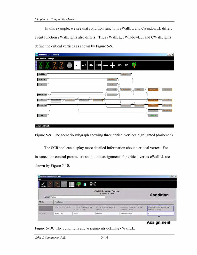
Chapter 5: Complexity Metrics
John J. Sammarco, P.E. 5-14
In this example, we see that condition functions cWallLL and cWindowLL differ;
event function cWallLights also differs. Thus cWallLL, cWindowLL, and CWallLights
define the critical vertices as shown by Figure 5-9.
Figure 5-9. The scenario subgraph showing three critical vertices highlighted (darkened).
The SCR tool can display more detailed information about a critical vertex. For
instance, the control parameters and output assignments for critical vertex cWallLL are
shown by Figure 5-10.
Figure 5-10. The conditions and assignments defining cWallLL.

Chapter 5: Complexity Metrics
John J. Sammarco, P.E. 5-15
Three Model Projections
Complex systems are multidimensional; thus, multiple projections (perspectives)
are needed. The problem of determining the proper projections for this research is
addressed by a simple partitioning of the system into the inputs and the outputs. We used
these partitions to define three projections for a given subgraph: 1) the all dependencies
projection; 2) the input projection; 3) the output projection.
The first projection named all, views all dependencies for a given subgraph. The
input projection views all descendents; the output projection views all ancestors. For
example, Figure 5-11 depicts a critical-vertex subgraph of the critical vertex mDefLSOpt.
Figure 5-11. The critical-vertex subgraph abstraction for vertex mDefLSOpt.
The input projection affords a view of dependencies with respect to inputs. We see
in Figure 5-11 that mDefLSOpt depends on two input vertices. Input vertices can change
values when environmental input conditions change or when users use the GUI to change
input parameters. For this example, the value of variable iOLSmalfuntion is determined
by a sensor malfunction; the value if variable iDefLSOpt is set by a human using a GUI.
The output projection enables a view of dependencies with respect to the outputs. We see

Chapter 5: Complexity Metrics
John J. Sammarco, P.E. 5-16
in Figure 5-11 that the critical vertex is a descendent of two output vertices as well as
three intermediate vertices.
The all projection looks at all dependencies associated with a given subgraph. In
the case of Figure 5-11, the all projection includes all dependencies of critical vertex
mDefLSOpt.
In summation, the input project enables a view of which inputs will affect the
critical vertices while the output projection enables a view of the outputs affected by the
critical vertices. The all projection is a collective view of all dependencies
Scenario Subgraph Metrics
The four metrics associated with the scenario subgraph are listed by Table 5-3.
Table 5-3. Coarse-grained metrics for the scenario subgraph abstraction. Metric Independent variable Projection
Cyclomatic complexity X1 all Output cyclomatic complexity X2 output All paths X3 all Graph degree X4 all
Each metric is described as follows:
X1 Cyclomatic complexity: McCabes cyclomatic complexity is calculated for the entire scenario subgraph. The subgraphs are weakly connected because dependency graphs are not connected from the output vertices to the input vertices. Adding a virtual edge from the output to input vertices will make the graph strongly connected (Vakil, 2000). Cyclomatic complexity is calculated as:
V (g) = e – n + (t +1) (5-3) where:
e = number of edges n = number of vertices t = number of output vertices
X2 Output cyclomatic complexity: This metric is an indicator of the common-mode connectivity of the output vertices. For instance, the output vertices of Figure 5-12 have common-mode connections because each output vertex is connected to the same input vertex.
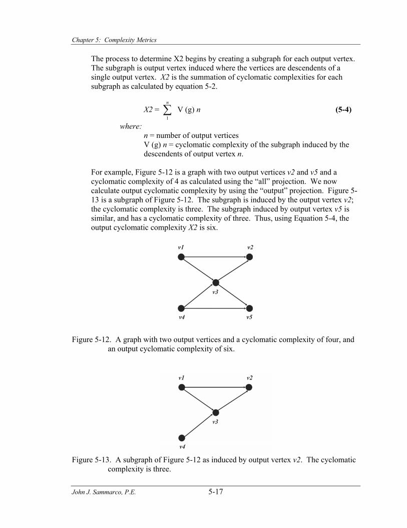
Chapter 5: Complexity Metrics
John J. Sammarco, P.E. 5-17
The process to determine X2 begins by creating a subgraph for each output vertex. The subgraph is output vertex induced where the vertices are descendents of a single output vertex. X2 is the summation of cyclomatic complexities for each subgraph as calculated by equation 5-2.
X2 = ∑n
1V (g) n (5-4)
where: n = number of output vertices V (g) n = cyclomatic complexity of the subgraph induced by the descendents of output vertex n.
For example, Figure 5-12 is a graph with two output vertices v2 and v5 and a cyclomatic complexity of 4 as calculated using the “all” projection. We now calculate output cyclomatic complexity by using the “output” projection. Figure 5-13 is a subgraph of Figure 5-12. The subgraph is induced by the output vertex v2; the cyclomatic complexity is three. The subgraph induced by output vertex v5 is similar, and has a cyclomatic complexity of three. Thus, using Equation 5-4, the output cyclomatic complexity X2 is six.
Figure 5-12. A graph with two output vertices and a cyclomatic complexity of four, and
an output cyclomatic complexity of six.
Figure 5-13. A subgraph of Figure 5-12 as induced by output vertex v2. The cyclomatic
complexity is three.

Chapter 5: Complexity Metrics
John J. Sammarco, P.E. 5-18
Figure 5-14 is another example; note that the graph has the same number of
vertices and it also has two output vertices. The cyclomatic complexity is 4 and is the
same as Figure 5-12. However, we see that output vertices do not have common-mode
connections so the cyclomatic complexity does not serve to measure the common-mode
connections for output vertices. The output cyclomatic complexity Figure 5-14 is two; a
significant reduction as compared to Figure 5-12.
Figure 5-14. A graph with two output vertices and a cyclomatic complexity of four, and
an output cyclomatic complexity of two.
X3 All paths: the maximum number of different directed paths. Each directed path
begins at an input vertex and ends at an output vertex. Additionally, each directed path must not be a strict semipath.
X4 Graph degree: the total number of graph edges because it equals the sum of all edges into and out of each vertex.
Critical-state Subgraph Metrics
The five metrics associated with the critical state subgraph, listed by Table 5-4, are
considered medium-grained metrics.
Table 5-4. The medium-grained metrics from the critical-state subgraph abstraction. Metric Independent variable Projection
Critical state changes X5 all In-degree X6 input Out-degree X7 output Cyclomatic complexity X8 all Sheppard complexity metric X9 all

Chapter 5: Complexity Metrics
John J. Sammarco, P.E. 5-19
X5 Critical-state changes: The critical-state subgraph is used to determine this metric. This metric indicates the number of nonlinear branching or interconnections where X5 is the number of variables that change for a single change of an input variable. Figure 5-7 serves as an example where X5 = 9.
X6 In-degree: The value of X6 is the summation of all edges going into the critical state subgraph vertices. For example, X6 = 9 for Figure 5-7. The X6 metric is from an input projection because looking from input to output vertices, we first encounter edges going into vertices.
X7 Out-degree: The value of X7 is the summation of all edges going out of the critical state subgraph vertices. For example X 7 = 9 for Figure 5-7. The X7 metric is from an output projection because looking from output to input vertices, we first encounter edges leaving vertices.
X8 Cyclomatic complexity: Metric X8 is calculated the same as metric X1. The difference is X8 is calculated from the critical state subgraph.
X9 Sheppard complexity metric: Metric X9 is a metric for interconnections where:
X9 = ( 6X x X )7 2 (5-5) where:
X5 = out-degree; X6 = in-degree.
Critical-vertex Subgraph Metrics
The six metrics associated with the critical-vertex subgraph are listed by Table 5-5. The metrics are described as follows: Table 5-5. Fine-grained metrics from the critical-vertex subgraph abstraction.
Metric Independent variable Projection In-degree X10 input Out-degree X11 output Sheppard complexity metric X12 all Input cyclomatic complexity X13 input Output cyclomatic complexity X14 output Vertex unique conditions X15 all X10 In-degree; X11 Out-degree; X12 Sheppard complexity: The metrics X10, X11, and
X12 are calculated the same as metrics X6, X7, and X9 respectively. Only the abstraction is different.
X13 Input cyclomatic complexity: The input projection is used to determine input cyclomatic complexity. The general process is the same as for the determination of output cyclomatic complexity. The input cyclomatic complexity is an indicator of common-mode connections for the input vertices.
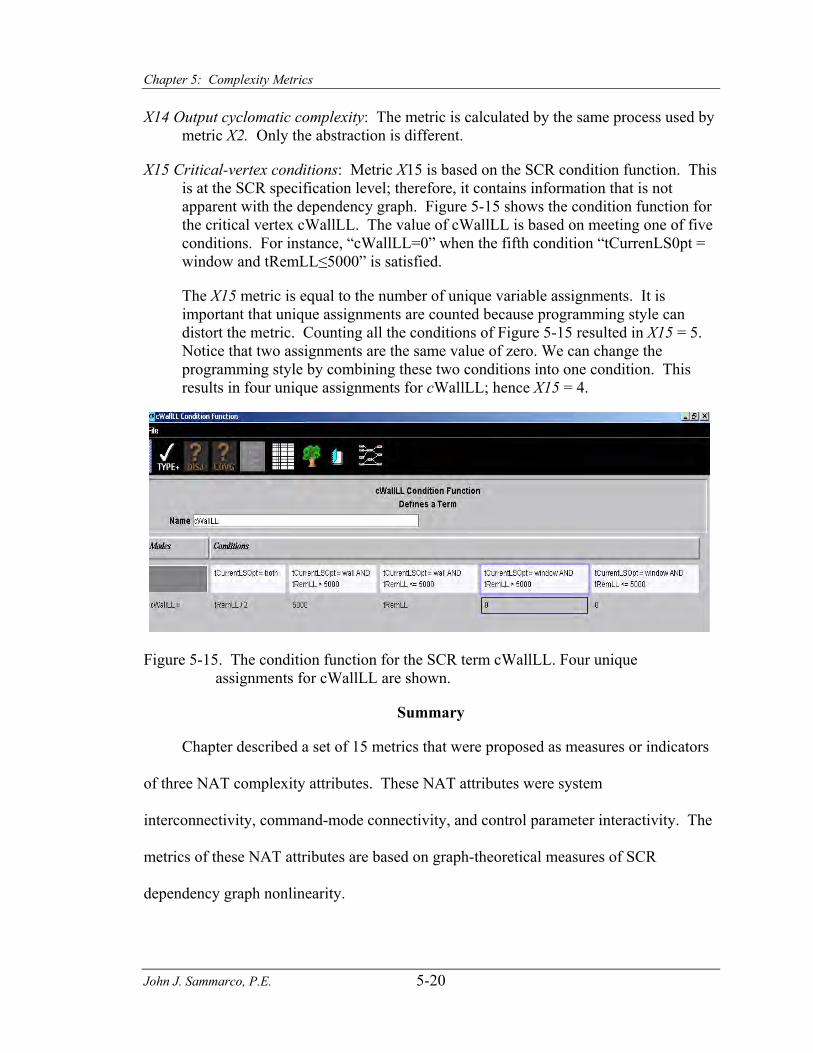
Chapter 5: Complexity Metrics
John J. Sammarco, P.E. 5-20
X14 Output cyclomatic complexity: The metric is calculated by the same process used by metric X2. Only the abstraction is different.
X15 Critical-vertex conditions: Metric X15 is based on the SCR condition function. This is at the SCR specification level; therefore, it contains information that is not apparent with the dependency graph. Figure 5-15 shows the condition function for the critical vertex cWallLL. The value of cWallLL is based on meeting one of five conditions. For instance, “cWallLL=0” when the fifth condition “tCurrenLS0pt = window and tRemLL≤5000” is satisfied.
The X15 metric is equal to the number of unique variable assignments. It is important that unique assignments are counted because programming style can distort the metric. Counting all the conditions of Figure 5-15 resulted in X15 = 5. Notice that two assignments are the same value of zero. We can change the programming style by combining these two conditions into one condition. This results in four unique assignments for cWallLL; hence X15 = 4.
Figure 5-15. The condition function for the SCR term cWallLL. Four unique
assignments for cWallLL are shown.
Summary
Chapter described a set of 15 metrics that were proposed as measures or indicators
of three NAT complexity attributes. These NAT attributes were system
interconnectivity, command-mode connectivity, and control parameter interactivity. The
metrics of these NAT attributes are based on graph-theoretical measures of SCR
dependency graph nonlinearity.
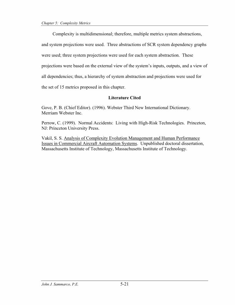
Chapter 5: Complexity Metrics
John J. Sammarco, P.E. 5-21
Complexity is multidimensional; therefore, multiple metrics system abstractions,
and system projections were used. Three abstractions of SCR system dependency graphs
were used; three system projections were used for each system abstraction. These
projections were based on the external view of the system’s inputs, outputs, and a view of
all dependencies; thus, a hierarchy of system abstraction and projections were used for
the set of 15 metrics proposed in this chapter.
Literature Cited
Gove, P. B. (Chief Editor). (1996). Webster Third New International Dictionary. Merriam Webster Inc.
Perrow, C. (1999). Normal Accidents: Living with High-Risk Technologies. Princeton, NJ: Princeton University Press.
Vakil, S. S. Analysis of Complexity Evolution Management and Human Performance Issues in Commercial Aircraft Automation Systems. Unpublished doctoral dissertation, Massachusetts Institute of Technology, Massachusetts Institute of Technology.
Chapter 6: Research Vehicle: The Light Control System (LCS)
John J. Sammarco, P.E
6-1
CHAPTER 6 RESEARCH VEHICLE: THE LIGHT CONTROL SYSTEM (LCS)
The LCS is a formalized system originally used to for requirements engineering
seminars. It is a moderately complex, real-world system that includes human-computer
interaction and safety requirements for normal and abnormal conditions.
The system is described in detail; this includes system functions, graphical user-
interface, and modifications to the system to correct a safety hazard and three ‘bugs” in
the original specification uncovered in this research. Additional modifications were
made to create six versions of the system needed for the research design described in the
next chapter.
Background
The LCS was devised by the Fraunhofer Institute for Experimental Software
Engineering in Kaiserslautern (Queins et al., 2000) for a seminar on Requirements
Capture, Documentation and Validation. The seminar was organized by E. Börger
(Universita di Pisa, I), B. Hörger (Daimler-Benz, Ulm, D), D. Parnas (McMaster
University, CAN), D. Rombach (Universität Kaiserslautern, D), with the objective to
compare different approaches for requirements elicitation and specification. The LCS
case study was used by the seminar as a vehicle to compare various requirements
engineering methods. The results were published in a special issue on Requirements
Engineering for the Journal of Universal Computer Science (Maurer, 2000).
The LCS specification, listed in Appendix A was based on the original version
created in 1995, and a subsequent 1999 version used in an earlier seminar on

Chapter 6: Research Vehicle: The Light Control System (LCS)
John J. Sammarco, P.E
6-2
Requirements Capture, Documentation, and Validation. The LCS specification created
for the 2000 seminar contains various improvements and refinements. The LCS
specification takes the form of an informal requirements document as created by the
customer. The requirements described functional requirements - the interactions between
the environment, humans, and the hardware/software of the system. The requirements
also state nonfunctional requirements - the constraints for the system such as timing and
performance restrictions.
System Description
The LCS was formulated as a moderately complex, real-world system to control the
interior lighting of a building consisting of various offices, laboratories, hallways, and
staircases. The system’s purpose is to efficiently control ambient lighting and to maintain
a safe environment. Seven requirements specifically concern safety aspects for normal
and abnormal conditions. For the purposes of this research, the control targets a single
office. The control other offices and laboratory spaces would be identical.
The operation of the LCS is detailed in the test subject instructions of Appendix E.
Briefly, the LCS controls light near the window and a light mounted near the wall. The
control enables the user to set two light scenes named occupied and vacant:
• Occupied light scene: Automatically maintains a user-defined lighting intensity and configuration when the office is occupied.
• Vacant light scene: Automatically provides a user-defined light intensity and configuration when someone enters the office after the vacant light scene time delay has expired.
Lastly, the LCS provides manual lighting control: Manual pushbuttons enable
on/off control of the lights. The manual controls enable users to over-ride the LCS

Chapter 6: Research Vehicle: The Light Control System (LCS)
John J. Sammarco, P.E
6-3
The LCS configuration for a single office is depicted by Figure 6-1. The system
components consist of sensors, a logic solver, wall and window light actuators, and a
user-interface panel. Five sensors are used; a motion sensor detects an occupied or
vacant office; an analog sensor measures natural light in the office; a door closed contact
indicates the door is open or closed; two status-line sensors indicate if the lights are
turned on or off. The logic solver is PC-based and it provides control functions and a
user-interface. Pushbutton switches enable manual and independent control of each light.
Figure 6-1. The Light Control System block diagram.
The LCS User-Interface
The PC-based user-interface, depicted by Figure 6-2, is used to set lighting scenes
and display system information. The user selects the lighting configuration (wall,
window, or both) and dimmer levels for the occupied and vacant light scenes. The user
also sets the time delay associated with the vacant light scene. The following status
information is displayed:
• Digital displays show the output for each light. No light is produced at 0 watts output; the maximum light is produced at 100 watts output.
• A digital displays shows elapsed time.
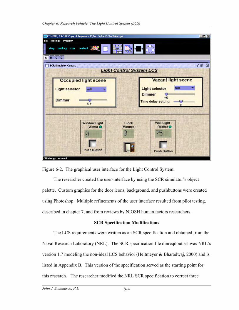
Chapter 6: Research Vehicle: The Light Control System (LCS)
John J. Sammarco, P.E
6-4
Figure 6-2. The graphical user interface for the Light Control System.
The researcher created the user-interface by using the SCR simulator’s object
palette. Custom graphics for the door icons, background, and pushbuttons were created
using Photoshop. Multiple refinements of the user interface resulted from pilot testing,
described in chapter 7, and from reviews by NIOSH human factors researchers.
SCR Specification Modifications
The LCS requirements were written as an SCR specification and obtained from the
Naval Research Laboratory (NRL). The SCR specification file dinreqdout.ssl was NRL’s
version 1.7 modeling the non-ideal LCS behavior (Heitmeyer & Bharadwaj, 2000) and is
listed in Appendix B. This version of the specification served as the starting point for
this research. The researcher modified the NRL SCR specification to correct three

Chapter 6: Research Vehicle: The Light Control System (LCS)
John J. Sammarco, P.E
6-5
undesirable behaviors found in the version 1.7 specification, and to obtain the required
behaviors for the test scenarios of this research.
The new SCR specification of this research consists of 15 monitored variables, 28
terms, eight controlled variables, one mode class, 24 conditioned functions, and 12 event
functions; thus, it was a moderately large specification.
The researcher's SCR specification modifications included two new output
variables named oWallOutput and oWindowOutput, were added to reduce system
complexity by mitigating inferential information for wall and window light outputs.
Perrow describes inferential information as a characteristic of a complex system. For
instance, the original SCR specification uses variable oDimmerWall to represent the wall
light intensity where zero watts gives no light and 100 watts gives maximum light. When
oDimmerWall equals 100 watts, it infers that light is producing the maximum light
output. However, the actual wall light output could be 0 watts. The oDimmerWall data
is inferential because important information is missing; specifically, the pulse signal
status as shown in Figure 6-2.
Each light is controlled by a dimmable light module that receives lighting demand
intensity from the dimmer input, and receives a pulse input enabling the light to be turned
off or on. The pulse is represented by the SCR variable oPulseWall. Therefore, if
oDimmerWall equal 100watts and oPulseWall equals 0 watts, no light is produced; if
oDimmerWall equals 100 watts and oPulseWall equals 1, and then light is produced.
Evidence of user confusion surfaced during LCS pilot testing. The pilot test GUI
used a virtual 4-digit LCD to show the values of oDimmerWall and oDimmerWindow.
The GUI also displayed on/off indicator lights for oPulseWall and oPulseWindow. The

Chapter 6: Research Vehicle: The Light Control System (LCS)
John J. Sammarco, P.E
6-6
research observed that some pilot test subjects focused on the LCD’s and did not observe
the state of oPulseWall or oPulseWindow indicator lights. For instance, pilot test
subjects found the externally visible behavior of the wall and window lights during the
wall and window light pushbutton scenario to be very confusing. This scenario used the
manually operated wall and window light pushbuttons to override the LCS control of
lighting. Users could manually shut off the wall or window light even though the LCS
was controlling the light at the desired intensity. The source of confusion is rooted in the
interrelationships between the manual pushbuttons and the variable pairs oDimmerWall
and oPulseWall, and oDimmerWindow and oPulseWindow. Table 6-1 summarizes the
nature of the relationships between oDimmerWindow, oPulseWall and the wall light
pushbutton. The relationships are identical for oDimmerWindow, oPulseWindow and the
window light pushbutton.
Table 6-1. Actual light output with respect to pulse and dimmer signal values. Wall light pushbutton state
oDimmerWall oPulseWall Actual wall light output
Off 100 0 (off) 0 Off 100 1 (on) 100 On 100 1 (on) 0
The actual wall light output is 0 regardless of the dimmer value specified by
oDimmerWall when the pulse signal oPulseWall is in the off state. Note also
oDimmerWall is independent of signal oPulseWall; this also caused user confusion
because pilot test subjects expected the dimmer value to equal zero if the pulse value was
zero. Therefore, the researcher created new variables, oWallOutput and
oWindowOutput, to represent the actual light output values. This eliminated subject

Chapter 6: Research Vehicle: The Light Control System (LCS)
John J. Sammarco, P.E
6-7
confusion during pilot test by using the same virtual 4-digit LCD to display the values of
oWallOutput and oWindowOuput on the GUI.
The researcher discovered a safety issue with the specified LCS behavior, and three
bugs with the NRL specification. These were discovered during the process of executing
the complexity assessment methodology of this research.
The safety issue concerns the fault tolerance requirement NFI, section (3.2.1.) of
the LCS problem description. This requirement can put the LCS in a state that creates a
hazard to the building’s occupants. Specifically, the requirement is for the LCS to use
the last known good datum from ambient light level sensor if the LCS detects a
malfunction of this sensor. This behavior causes a hazard because people could enter a
dark office without the lighting coming on. This hazard occurs when the ambient light
sensor malfunctions during very bright ambient light levels where the naturally occurring
light provides all the lighting requested by the user; thus, the wall and window lights are
reduced to 0 watts output. The specified behavior during the malfunction causes the
system to use this high light level because it was the last known value before the
malfunction. Hence, users entering an office at night after a malfunction has occurred
during these high level lighting conditions will find the office dark because the LCS
system believes ambient light is providing all the lighting needed. The researcher
collaborated with experts from the NRL to correct this problem. The first correction was
to modify the indoor lighting level monitoring function so that it assumes it is dark
outside in the case of a malfunction lighting sensor. This essentially would be a failsafe
state because lighting would always be available. The second fix to this problem was to
have the ambient light sensor re-read after an ambient light sensor malfunction so that the

Chapter 6: Research Vehicle: The Light Control System (LCS)
John J. Sammarco, P.E
6-8
latest reading can be used. Without this, the value before the failure would remain in the
system until the sensor reading changed again and the malfunction was cleared.
The three bugs with the SCR specification are not safety related but, do cause
undesirable behavior that could confuse the occupants of the building. The first and
second problems are related to the initial state of the system. The third bug concerns the
ambient light level sensor.
The first problem concerns the light status of the room when someone first enters
the room. The LCS problem description specified that upon the first time a room is
entered that the default light scene should be on. This did not occur during the execution
of the LCS specification by NRL. The second problem is also related to this initial state.
This problem however does have safety implications. Under the right conditions, the
LCS control system would shut off all the lights in the office even though the office was
occupied and lighting was called for. The system will erroneously go to an unoccupied
state two minutes after a person enters an office for the first time. At this point, the
system is in a temporarily empty state classification. Therefore a timer associated with
the temporary empty state begins counting, and once this timer elapses, the lighting will
be shutoff to the office even though an operator or a user is in the room. The third
problem that occurs is that the current dimmer outputs do not correctly account for the
natural light entering the room for any given state.
Again the researcher collaborated with NRL personnel to correct these three
problems. At this point, this brings us to the SCR specification, designated as treatment
A, containing the corrections for the three NRL bugs and the undesirable safety behavior
specified in the LCS specification.

Chapter 6: Research Vehicle: The Light Control System (LCS)
John J. Sammarco, P.E
6-9
Scenario Descriptions
Three scenarios were designed to exercise all of the major LCS functions. More
importantly, the scenarios are based on LCS behavior the researcher found to exhibit
NAT characteristics of confusion, transparency, and unpredictable system behavior.
Therefore, the researcher began with the complex system, designated as treatment A, then
simplified the system and designated this as treatment B. Two treatments are needed to
test the research hypotheses. The next chapter details the research methodology for
treatments A and B.
The Vacant Light Scene Scenario
The vacant light scene is used to maintain safety and save energy. It provides a
minimal lighting level when a user enters an office. The scene helps save energy by
reducing the lighting once the office has been vacated for longer than a user-defined time
delay; therefore, if a person does not shut off the lights when leaving the office, the LCS
will automatically reduce the lighting level once the time delay expires. The vacant light
scene settings are defined and set by the user
Appendix E contains the detailed subject instructions for the vacant light scene
scenario. Subjects are instructed to set the vacant light scene to the window light at 20
watts, with a time delay of five minutes. After the scene is set, the subject leaves the
office, and advances time from zero to seven minutes while watching the state of the
vacant light scene. The subject reoccupied the office at seven minutes and observed the
vacant light scene settings.
The vacant light scene scenario for treatments A and B is summarized by Table 6-
2. The items of primary interest are in bold. The first critical time is at five minutes, the

Chapter 6: Research Vehicle: The Light Control System (LCS)
John J. Sammarco, P.E
6-10
time delay setting. Note that the LCS behavior for treatments A and B are identical up to
the time delay setting of five minutes. The vacant light scene activated at five minutes
and remained activated for treatment B, the less complex system. Therefore, the vacant
light scene was on when the subject reoccupied the office. The behavior for treatment A
differed in that the vacant light scene did not activate until the subject re-entered the
office at seven minutes.
Table 6-2. Vacant light scene scenario values for treatment A and B. The items of primary interest are in bold.
Time (Minutes)
LCS Mode
Light Scene
Treatment A Vacant Light (Window)
Treatment B Vacant Light (Window)
0 occupied occupied disabled disabled 1 temp.
empty occupied disabled disabled
2 temp. empty
occupied disabled disabled
3 temp. empty
occupied disabled disabled
4 temp. empty
occupied disabled disabled
5 (delay time value)
temp. empty
vacant
disabled
enabled @ 20 watts
6 temp. empty
vacant disabled enabled @ 20 watts
7 occupied vacant enabled @ 20 watts enabled @ 20 watts The Lighting Options Scenario
This scenario demonstrates the operation of the lighting options. The lighting
options are wall lights, window lights, or both lights. The lighting options are selected by
the user. Appendix E contains the detailed subject instructions for the lighting options
scenario.

Chapter 6: Research Vehicle: The Light Control System (LCS)
John J. Sammarco, P.E
6-11
Section 4 is the dictionary of terms for the LCS requirements. The operation of
each lighting option is defined within the definition of the light scene term. The light
scene definition follows; italics were added for emphasis:
A light scene is a predefined setting of the ambient light level and a description that determines in which way the ceiling light groups should be used to achieve this ambient light level. A light scene is given by:
1. name of the light scene
2. the desired ambient light level in a room
3. one of the following three options: window, wall, or both
Window means that at first the ceiling light group near the window should be used to achieve the desired ambient light level and then the other ceiling light group.
Wall means that at first the ceiling light group near the wall should be used to achieve the desired ambient light level and then the other ceiling light group.
Both means that both ceiling light groups should be used equally to achieve the desired ambient light level (Queins et al., 2000).
If the requested level of light can not be supplied by a single light, then the LCS
automatically supplies power to the other light in order to meet the request. Each light
provides up to 100 watts. So, if the wall light is selected, and the requested light level is
150 watts, then the LCS automatically controls the window light to provide 50 watts,
even though the user requested only the wall light. The outputs for treatment A are listed
by Table 6-3, and depict the situation when the dimmer is set to 7,500. Treatment B
differs by not automatically shifting part of the lighting demand to the window light.

Chapter 6: Research Vehicle: The Light Control System (LCS)
John J. Sammarco, P.E
6-12
Table 6-3. Lighting options scenario values for treatment A and B. The items of primary interest are in bold.
Dimmer Settings
Treatment A Treatment B
Wall
Window
Wall Output (Watts)
Window Output (Watts)
Wall Output (Watts)
Window Output (Watts)
0 0 0 0 0 0 2,500 0 50 0 50 0 5,000 0 100 0 100 0 7,500 0 100 50 100 0 10,000 0 100 100 100 0 7,500 0 100 50 100 0 5,000 0 100 0 100 0 2,500 0 50 0 50 0 0 0 0 0 0 0 The Wall and Window Light Pushbutton Scenario
This scenario demonstrates the operation of the light pushbuttons. The manually
operated wall and window light pushbuttons are used to override the LCS. Manual
override of the LCS control occurs when the window pushbutton state is “on.” Appendix
E contains the detailed subject instructions for the wall and window light pushbutton
scenario.
Requirement 2 of section 2.1 of the LCS problem description, defines the behavior
for the pushbuttons. It states:
Each office is equipped with:
1. one motion detector (imd), so that the room is fully covered.
2. two ceiling light groups (window and wall).
The luminaries in a ceiling light group in any room are turned on or off only as a group. Each ceiling light group is controlled by one push button on the wall (pb1 and pb2, respectively), which toggles the ceiling light group if pushed.
A ceiling light group in a room shows the following behavior if the corresponding push button is pushed:

Chapter 6: Research Vehicle: The Light Control System (LCS)
John J. Sammarco, P.E
6-13
(i) if the ceiling light group is completely on, it will be switched off
(ii) otherwise it will be switched on completely (Queins et al., 2000).
Table 6-4 depicts the operation of the window light pushbutton for treatments A
and B. Note that both treatments behave identically until the last table entry (in bold).
Treatment A did comply with the specification although this is not intuitive; also, it does
not follow the functional mental model most people have concerning a pushbutton switch
found in homes and offices.
When the prior state is window output = 50 watts, the window light is not fully on.
So, when the window pushbutton changes to the on state, the current state becomes
window output’ = 100 watts. For treatment B, window output’ = 0 watts; this behavior
follows the typical functional mental model for a pushbutton light switch.
Table 6-4. Wall and Window light pushbutton scenario outputs for treatments A and B. The items of primary interest are in bold.
Treatment A
Treatment B Window pushbutton Window output
(Watts) Window output’ (Watts)
Window output (Watts)
Window output’ (Watts)
off 0 0 0 0 on 0 100 0 100 off 100 100 100 100 on 100 0 100 0 off 50 50 50 50 on 50 100 50 0 Note: Window output’ is the current state value while window output is the prior state value

Chapter 6: Research Vehicle: The Light Control System (LCS)
John J. Sammarco, P.E
6-14
Summary
The research test vehicle is the LCS, a formally documented system used as a case
study for requirements engineering seminars. The function behavior of the LCS was
described as well as the GUI created for human interaction with the LCS. This research
modified the LCS behavior to mitigate a safety hazard and three bugs in the original LCS
as constructed as an SCR specification. Next, the LCS specification was modified to
generate two treatments for three scenarios named the vacant light scene, the lighting
options scenario, and the wall and ceiling light push button scenario. Treatment A of
these scenarios follows the LCS specifications. Treatment B is made to be more intuitive
and to match typical functional mental models. The treatments and scenarios are used to
test the research hypotheses. The next chapter explains how these treatments and
scenarios are used in the research methodology.
Literature Cited
Heitmeyer, C., & Bharadwaj, R (2000) Applying the SCR Requirements Method to the Light Control Case Study. Journal of Universal Computer Science; Special Issue on Requirements Engineering, Vol. 6, No. 7.
Maurer, H. (Ed.). (2000). Journal of Universal Computer Science (Vol. 6. No. 7). Springer Publishing Company.
Queins, S., Zimmerman, G., Becker, M., Kronengurg, M., Peper, C., Merz, R., & Schafer, J. (2000). The Light Control Case Study: Problem Description. Journal of Universal Computer Science; Special Issue on Requirements Engineering, Vol. 6, No. 7.

Chapter 7: Research Methodology
John J. Sammarco, P.E
7-1
CHAPTER 7 RESEARCH METHODOLOGY
This chapter describes the specific tasks, sequences, and research methodology
needed to realize the research objective: to develop a complexity assessment
methodology for system requirements of safety-related e computer systems by
operationalizing NAT.
A multiple data source approach was taken to increase construct validity. The
research included the use of the Discount Usability Engineering method to evaluate
system usability, and a crossover research design to obtain multidimensional data from
two sources: a questionnaire instrument for the test subjects and observer notes
Thirty-two convenience subjects from the NIOSH Pittsburgh Research Laboratory
used PC-based simulations of the LCS described in chapter 6. The subjects were
randomly assigned to execute scenarios that used the main functions of the LCS. The
nine-part questionnaire instrument of Appendix D was used for the collection of
dependent variable data. Three dependent variables were measured using a five-point
Likert scale.
Lastly, six subjects were used to conduct pilot tests. This resulted in improvement
and refinement of the subject instructions and the GUI; specifically, the instructions were
shorter, easier to follow, and easier to understand; the GUI was simplified to make it
more intuitive.

Chapter 7: Research Methodology
John J. Sammarco, P.E
7-2
Experiment Overview
This experiment consisted of two major parts having a total of six steps. The first
part was to teach subjects about the LCS. This was achieved in three steps:
• Watch a short instructional video concerning the operation of the LCS; • Read a description of the GUI and the operating instructions for the LCS; • Receive “hands-on” training by using the basic LCS functions during a 10minute
warm-up session. For the second part, the subjects:
• Followed a one page set of instructions to run a scenario; • Answered the questionnaire after running each scenario; • Take a one-minute break after running each scenario.
Research Design
The research used the Discount Usability Engineering method to evaluate the
usability of the LCS. The usability was evaluated for a warm-up session and six
scenarios of LCS operation.
The research design uses a crossover design. The main advantages of using
standardized designs and methods are pre-established validity and a prior knowledge of
strengths and limitations.
Discount Usability Engineering
The Discount Usability Engineering method was used to evaluate system usability:
one of our dependent variables. A strong point of this method is that it can maximize
data significance given small sample population sizes. Nielsen's research shows that
three to five subjects achieves the maximum benefit-cost ratio for this method (Nielsen,
1994). Secondly, the method's simplicity was an advantage. It was much less likely that
error and biases are introduced from misapplication of complex methods.

Chapter 7: Research Methodology
John J. Sammarco, P.E
7-3
The Discount Usability Engineering method uses three techniques: scenarios,
simplified thinking aloud, and heuristic evaluation. A scenario contains a set of events,
tasks, and operations typically encountered in the system operation. A scenario can
consist of normal or abnormal situations. The simplified thinking aloud technique
encourages the subjects to vocalize their thoughts as they perform typical tasks.
Researchers record these thoughts and encourage the users to vocalize their thoughts and
provide user feedback.
A crossover design was used to compare difficult and easy scenarios using within
subject comparisons and allowing for multiple evaluations per subject. This research
design is commonly used for clinical drug studies.
Crossover Design
The crossover design has a significant advantage because the subjects serve as their
own control. The other advantages include greater sample size efficiency with
randomization of treatment order and all subjects receive all the treatments. The basic
structure of a crossover design is depicted by Figure 7-1. Randomly, half of the subjects
received treatments in a given order while the other half received the same treatments in
reverse order. A washout or waiting period was established between treatments to
minimize carryover or residual learning effects from the prior treatments. The washout
duration varies with respect to the specific study. For example, drug studies could have
washout periods ranging from hours to days depending upon how quickly a drug leaves
the bloodstream. Lengthy or unknown washout periods are a disadvantage; however, the
washout period used in this research was just a few minutes because the residual effects
are not physiological. Short washout periods are needed because of practicality.
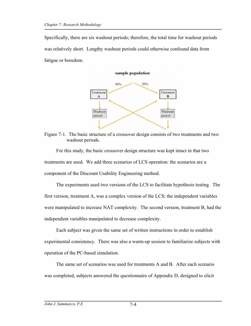
Chapter 7: Research Methodology
John J. Sammarco, P.E
7-4
Specifically, there are six washout periods; therefore, the total time for washout periods
was relatively short. Lengthy washout periods could otherwise confound data from
fatigue or boredom.
Figure 7-1. The basic structure of a crossover design consists of two treatments and two
washout periods.
For this study, the basic crossover design structure was kept intact in that two
treatments are used. We add three scenarios of LCS operation: the scenarios are a
component of the Discount Usability Engineering method.
The experiments used two versions of the LCS to facilitate hypothesis testing. The
first version, treatment A, was a complex version of the LCS; the independent variables
were manipulated to increase NAT complexity. The second version, treatment B, had the
independent variables manipulated to decrease complexity.
Each subject was given the same set of written instructions in order to establish
experimental consistency. There was also a warm-up session to familiarize subjects with
operation of the PC-based simulation.
The same set of scenarios was used for treatments A and B. After each scenario
was completed, subjects answered the questionnaire of Appendix D, designed to elicit

Chapter 7: Research Methodology
John J. Sammarco, P.E
7-5
their perceptions of the system. The responses were assumed to depend on the assigned
treatment.
Two structured test sequences of scenarios and treatments were used to establish
known test patterns; one test sequence was used by half of the subjects and the other test
sequence was used by the other half. The test sequences of scenarios and treatments were
optimized for the crossover design (Jones & Kenward, 1998). Tables 7-1 and 7-2 list the
test sequences with their associated scenarios and treatments. .
Table 7-1. Sequence 1 ordering of the scenarios and associated treatments.
Order Scenario Treatment 0 warm-up session 1 washout period 2 1 A 3 washout period 4 2 B 5 washout period 6 3 A 7 washout period 8 2 A 9 washout period 10 1 B 11 washout period 12 3 B
Table 7-2. Sequence 2 ordering of the scenarios and associated treatments.
Order Scenario Treatment 0 warm-up session 1 washout period 2 3 B 3 washout period 4 1 B 5 washout period 6 2 A 7 washout period 8 3 A 9 washout period 10 2 B 11 washout period 12 1 A
The two sequences were useful for detecting and limiting learning effects by
reducing the potential learning effects to a subset of known scenario and treatment
ordering. A totally randomized sequence of scenarios could potentially have a wider
range of learning effects thus making it more difficult to address.

Chapter 7: Research Methodology
John J. Sammarco P.E
7-6
Internal Validity Threats
The research methodology was also designed to reduce potential threats to internal
validity. Compromises of internal validity result in biases that cloud inferences
concerning the observed effects that the independent variables may have on the
dependent variables. Internal validity considerations included construct validity and
unintended treatment effects. The following steps were made integral to the research to
increase internal validity:
• Construct validity:
o Used multidimensional data;
o Used multiple data sources;
• Unintended non-experimental effects (a.k.a. Hawthorn effect): Independent observers were used to proctor tests and collect data
Warm-up Session
All subjects receiving treatments A and B conducted the same warm-up session
prior to conducting the LCS test. The warm-up served as a hands-on practice session.
The objectives of this session were to help subjects become familiar with running a
scenario and become familiar with using the GUI. The subjects answered a set of
questions concerning each of these objectives after they completed the warm-up session.
Test Sequence Summary
The test sequences are summarized using the appropriate statistical terminology as follows: • 2 Sequences: Tables 7-1 and 7-2 describe the sequences.
• 2 Treatments: Treatment A (more complex), Treatment B (less complex)
• 3 Periods: Scenarios 1, 2, 3 (each scenario was a set of typical user tasks)

Chapter 7: Research Methodology
John J. Sammarco, P.E
7-7
Observers
Three volunteers from the NIOSH Pittsburgh Research Laboratory were test
observers: they were used to administer the tests and collect data. The observers did not
know the purpose of the research or understand the operation of the LCS. This was an
intentional part of the design so as to reduce the potential for observer-induced biases.
Observers took notes about each subject; the notes contained observations on the
subject’s verbal comments, actions, and body language during the test.
Subjects
The research includes the use of human subjects; therefore, the methodology
required review by the West Virginia University Institutional Review Board (IRB) for the
protection of human subjects. Due to the minimal risk of the tests, an exemption was
requested and granted. Appendix C contains the exception request and IRB approval.
A total of 41 subjects from the NIOSH Pittsburgh Research Laboratory
volunteered to participate in this study. Six of these subjects participated in pilot testing;
32 subjects participated in the LCS tests; three served as test observers. All subjects were
recruited as volunteers by word of mouth from researchers from NIOSH, Pittsburgh
Research Laboratory.
Measurement Methods
Two methods are used to collect dependent variables: the think-aloud protocol of
Discount Usability Engineering method and the questionnaire instrument of Appendix D.
Questionnaire Instrument
Table 7-3 maps the dependent variables to the specific questionnaire sections.
Portions of the questionnaire are from two respected and validated instruments: the

Chapter 7: Research Methodology
John J. Sammarco, P.E
7-8
Questionnaire for User Interaction Satisfaction (QUIS) and the Software Usability
Measurement Inventory (SUMI).
Table 7-3. The dependent variables and corresponding sections of the questionnaire. Dependent Variable Questionnaire Sections Predictability (p) 3.1.1, 3.1.2, 3.1.3, 3.2 Observability (o) 3.3.1, 3.3.2, 3.4, 3.5, 3.6 Usability (u) 3.7, 3.8, 3.9, 3.10
QUIS is used to Aprovide researchers with a validated instrument for conducting
comparative evaluations, and serve as a test instrument in usability labs@ (Human
Computer Interaction Laboratory, 2002).
SUMI is Aa rigorously tested and proven method of measuring software quality
from the end user's point of view@ and Aas the de facto industry standard questionnaire”
(Human Factors Research Group, 2002). The international standard ISO 9241 recognizes
the SUMI method to test user satisfaction.
The validity of the QUIS and SUMI surveys was kept intact by using a two-step
adaptation process. The first step Afilters@ for questions pertaining to this research. The
second step Afocuses@ the questions explicitly to this research. For instance, a question
with Athis software@ was reworded to Athis system@.
Each subject completes the questionnaire to elicit their perceptions. The
questionnaire uses multiple choice and open-ended questions. The multiple-choice
questions are based on a five-point Likert scale. Open-ended questions are used to
collect post-experimental data for the experiment at the conclusion of the entire sequence.
Observer Notes
The think-aloud technique yielded qualitative data as recorded by an observer
during subject testing. The data was recorded in the form of written observations of the

Chapter 7: Research Methodology
John J. Sammarco, P.E
7-9
subject’s verbal and nonverbal communications during the tests. This qualitative data
was another component assumed to be dependent on the treatment, adding another
dimension to dependent variable data from the perspective of the observer.
Pilot Testing
The main objective of pilot testing was to identify and correct the weaknesses and
shortcomings with the LCS instructions, test scenario instructions, and the graphical user
interface (GUI) before conducting LCS tests with 32 subjects. Six convenience subjects
volunteered to conduct pilot testing: these subjects did not participants in LCS tests.
The pilot testing proved to be very beneficial. It resulted revising the instructions
to make them shorter and easier to follow and understand. It also resulted in a simpler,
more intuitive GUI.
Subject Instructions
Subjects received written instructions for the operation of the LCS and for
executing the tasks of each scenario. There was considerable variation in subject
comprehension, subject errors, and with the expected subject actions and behaviors.
Many instruction-related issues were found to be dependent on the form or method of
delivering instructions. It was also evident that using written instructions alone would
not suffice for a group of 32 subjects because of the variability in the way people learn.
For instance, some people learn best by reading while others learn by listening; yet others
learn by doing. Realistically, people learn in various combinations of these. Hence,
instructions were delivered by multiple methods as described:
• LCS instruction improvements: The information was presented in four forms to accommodate subjects who learn by reading, watching, listening, and by doing. First, subjects watched a PowerPoint presentation having pre-recorded narratives. The presentation gave an overview of the process and the operation of the LCS, which also contained a video file of the researcher executing the warm-up sessions.

Chapter 7: Research Methodology
John J. Sammarco, P.E
7-10
These provided a dynamic example of using the LCS GUI, and using the read-aloud and think-aloud techniques.
• Scenario instruction improvements: The researcher observed that errors of omission were predominant and that most subjects had difficult comprehending the scenarios. Subjects were merely following instructions so they did not closely observe or understand LCS behavior. Changing the instructions in two ways provided an improvement. The first was to rewrite the scenario instructions changing from a sequence of operator tasks to a set of instructions that establish an objective within the context of a story. Therefore, each instructed task had more meaning for subjects because they could place the tasks within the context of the scenario’s objective.
• Subject comprehension and errors of omission improvements: It appeared that subjects were reading instructions too quickly. To remedy this, subjects were asked to read the instructions out loud. This activity slowed down and focused the subject’s thoughts on the instructions. The researchers observed these benefits:
o eliminated errors of omission;
o improved subject comprehension;
o increased subject vocalizations during the think aloud technique;
o facilitated observer data collection because it was easier to follow and record subject observations;
o facilitated observations because it gave observers an additional data source; for example, as the subject read the instructions, an observer could infer as source of confusion to be with the instructions.
The researcher’s “read-aloud” technique was an effective solution for the scenario
instruction issues, and it provided additional benefits. The read-aloud technique had
merit for this research. Additional investigation into the effectiveness of the read-aloud
technique is needed.
Graphical User Interface Improvements (GUI)
The original user interface grouped interface controls by categories. For instance,
the dimmer slide controls were grouped together and the lighting option pull down menus
were grouped together. Subjects found this cumbersome and non-intuitive.

Chapter 7: Research Methodology
John J. Sammarco, P.E
7-11
The researcher’s solution was to group interface controls by LCS functions.
Specifically, the user interface groupings were the occupied light scene, vacant light
scene, and window and wall light groups.
Data Preparation
Dependent Variables
Each dependent variable has a quantitative component: obtained from the subject
questionnaire ratings, and a qualitative component: obtained from written observations
of each subject during tests.
The raw dependent data for the three scenarios was entered from the questionnaire
into a single Excel spreadsheet. Columns were also added for each dependent variable.
These columns contained the mean subject ratings of predictability, observability, and
usability for each subject.
Qualitative Data
Qualitative data was quantified by using a process of categorizing and mapping
the data to a five-point Likert scale as used by the subject questionnaire. This process is
depicted in figure 7-2. Once the observer data was quantified, the mean values for each
category was weighted by 30%, then combined with questionnaire data for dependent
variables p, o, and u.
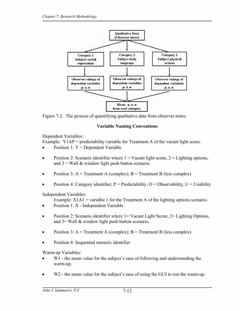
Chapter 7: Research Methodology
John J. Sammarco, P.E
7-12
Figure 7-2. The process of quantifying qualitative data from observer notes.
Variable Naming Conventions
Dependent Variables: Example: Y1AP = predictability variable for Treatment A of the vacant light scene. • Position 1: Y = Dependent Variable
• Position 2: Scenario identifier where 1 = Vacant light scene, 2 = Lighting options, and 3 = Wall & window light push button scenario.
• Position 3: A = Treatment A (complex); B = Treatment B (less complex)
• Position 4: Category identifier; P = Predictability, O = Observability, U = Usability
Independent Variables: Example: X1A1 = variable 1 for the Treatment A of the lighting options scenario.
• Position 1: X - Independent Variable
• Position 2: Scenario identifier where 1= Vacant Light Scene, 2= Lighting Options, and 3= Wall & window light push button scenario.
• Position 3: A = Treatment A (complex); B = Treatment B (less complex)
• Position 4: Sequential numeric identifier
Warm-up Variables: • W1 - the mean value for the subject’s ease of following and understanding the
warm-up.
• W2 - the mean value for the subject’s ease of using the GUI to run the warm-up.

Chapter 7: Research Methodology
John J. Sammarco, P.E
7-13
Summary
The experimental method and plan were presented. The research design was based
on a cross-over design; a standard design with an established validity. The research also
used a standard usability evaluation method: the Discount Usability Engineering method.
Our research methodology and plan addresses the test subjects, measurement methods,
data collection and preparation, and the statistical analyses. Lastly, the threats to internal
validity are recognized and addressed.
Literature Cited
Human Computer Interaction Laboratory. QUIS [Web Page]. URL http://www.cs.umd.edu/hcil/quis/ [2002, February 7].
Human Factors Research Group. (SUMI Homepage [Web Page]. URL http://www.ucc.ie/hfrg/questionnaires/sumi/index.html [2002, February 7].
Jones, B., & Kenward, M. G. (1998). Design and Analysis of Cross-Over Trials. Chapman and Hall.
Nielsen, J. (1994). Guerrilla HCI: Using discount usability engineering to penetrate the intimidation barrier. In R. G. Bias, & D. J. E. Mayhew Cost-Justifying Usability (pp. pp. 245-272). Boston, MA: Academic Press.

Chapter 8: Data Analyses and Hypotheses Testing
John J. Sammarco, P.E
8-1
CHAPTER 8 DATA ANALYSES AND HYPOTHESES TESTING
The previous chapter described the research methodology used to conduct tests.
This chapter details the analysis of test data and the hypotheses testing. Descriptive
statistics of median and mode, and histograms were used to characterize the test subjects,
the results of warm-up tests, and the main test results. Next, data validity was addressed
by analyzing subject data for outliers, by conducting data reliability estimates, and by
investigating data trends for evidence of data confounding.
Once data validity was established, nonparametric statistical methods were used to
test the hypotheses. Canonical correlation analysis and structure correlations were used
determine what linear combination of dependent variables was most strongly correlated
with a linear combination of independent variables. The results pertain to null
hypotheses 1 through 3 − the dependent variables predictability, observability, and
usability do not correlate with our NAT metrics of complexity. The Wilcoxon signed-
rank test was used to test hypotheses 4 through 6 − increasing NAT complexity does not
decrease system predictability, observability, and usability.
Lastly, the results of statistical tests were determined through the calculation of p-
values, standard errors, and 95% confidence intervals.
Subject Profiles
Thirty-two volunteer subjects from the National Institute for Occupational Safety and
Health, Pittsburgh Research Laboratory participated in testing. The subjects had no prior
knowledge or involvement of this research. Each subject responded to all questions for

Chapter 8: Data Analyses and Hypotheses Testing
John J. Sammarco, P.E
8-2
Part 1 of the questionnaire instrument of Appendix D. The typical subject is
characterized as follows based upon subject data collected during pre-test activities:
• 78.1% - technical job classification; • 71.8% - 45-65 years old; • 87.3% - male; • 100% - no prior involvement in the research; • 84.4% - no knowledge of the light control system test vehicle; • 84.4% - PC experience rated at 4 or 5 (expert). Figure 8-1. characterizes subjects in more detail. Each x-axis item represents a question from part 1 of the subject questionnaire of Appendix D.
0
5
10
15
20
25
30
35
Tech
Non
-Tec
h
18-2
4
25-3
4
35-4
4
45-6
5
Mal
e
Fem
ale
Yes No
Kno
w L
evel
1
Kno
w L
evel
2
Kno
w L
evel
3
Kno
w L
evel
4
Kno
w L
evel
5
Exp
Lev
el 1
Exp
Lev
el 2
Exp
Lev
el 3
Exp
Lev
el 4
Exp
Lev
el 5
Subject Dimension
Res
pons
es
Job Type: Technical(Tech) and Non-Technical(Non-Tech)Age Range
Gender
Involved in this research?
LCS Knowledge: 1 =none, 5 = expert
PC Experience : 1 = none,5 = expert
Figure 8-1 Subject profile data from the subject questionnaire of Appendix D.
Subject Responses for the Warm-Up Session
Two measurements were used to characterize the subject’s perceptions of the
overall warm-up session. W1 is a measure of the subject’s ease of following and
understanding the warm-up instructions. W1 was calculated as the mean of 28 subject

Chapter 8: Data Analyses and Hypotheses Testing
John J. Sammarco, P.E
8-3
ratings for questions 2.1.1 to 2.1.4 of the questionnaire. Figure 8-2(A) depicts the
histogram for W1. W2 represents the subject’s ease of using the GUI. W2 measures the
subject’s ease of using the GUI to run the warm-up. W2 was calculated as the mean of
28 subject ratings for questions 2.2 to 2.6 of the questionnaire. Figure 8-2(B) depicts the
histogram for variable W2.
(low) Mean Rating of Warmup (high)
4.994.463.943.412.892.361.841.31.79.26
(A)
Variable W1
Freq
uenc
y
14
12
10
8
6
4
2
0
(low) Mean Rating of GUI (high)
5.234.684.133.583.032.481.931.38.83.28
(B)
Variable W2
Freq
uenc
y
14
12
10
8
6
4
2
0
Figure 8-2. Mean subject responses for the warm-up session. Graph (A) depicts the
subjects understanding of session tasks. Graph (B) depicts the subject’s ease of using the GUI.
Test Data Characterizations
A more detailed depiction of subject responses is presented by a series of
histograms. The frequency of responses for each scenario and treatment are depicted by
the histograms of Figures 8-3, 8-4, and 8-5

Chapter 8: Data Analyses and Hypotheses Testing
John J. Sammarco, P.E
8-4
Treatment A Treatment B
(low) Mean Predictability (high)
5.004.473.953.422.892.371.841.32.79.26
(A)
Variable Y1AP
Freq
uenc
y
121110
9876
543
210
(low) Mean Predictability (high)
5.004.473.953.422.892.371.841.32.79.26
(B)
Variable Y1BP
Freq
uenc
y
12
10
8
6
4
2
0
(low) Mean Observability (high)
5.004.504.003.503.002.512.011.511.01.51
(C)
Variable Y1AO
Freq
uenc
y
12
10
8
6
4
2
0
(low) Mean Observability (high)
5.004.504.003.503.002.512.011.511.01.51
(D)
Variable Y1BO
Freq
uenc
y12
10
8
6
4
2
0
(low) Mean Usability (high)
5.004.504.003.503.002.512.011.511.01.51
(E)
Variable Y1AU
Freq
uenc
y
12
10
8
6
4
2
0
(low) Mean Usability (high)
5.004.504.003.503.002.512.011.511.01.51
(F)
Variable Y1BU
Freq
uenc
y
12
10
8
6
4
2
0
Figure 8-3. The mean predictability, observability, and usability responses for the vacant
light scene scenario. Graphs (A), (E), and (D) depict treatment A responses; graphs (C), (B), and (F) depict treatment B responses. N = 28 subjects.
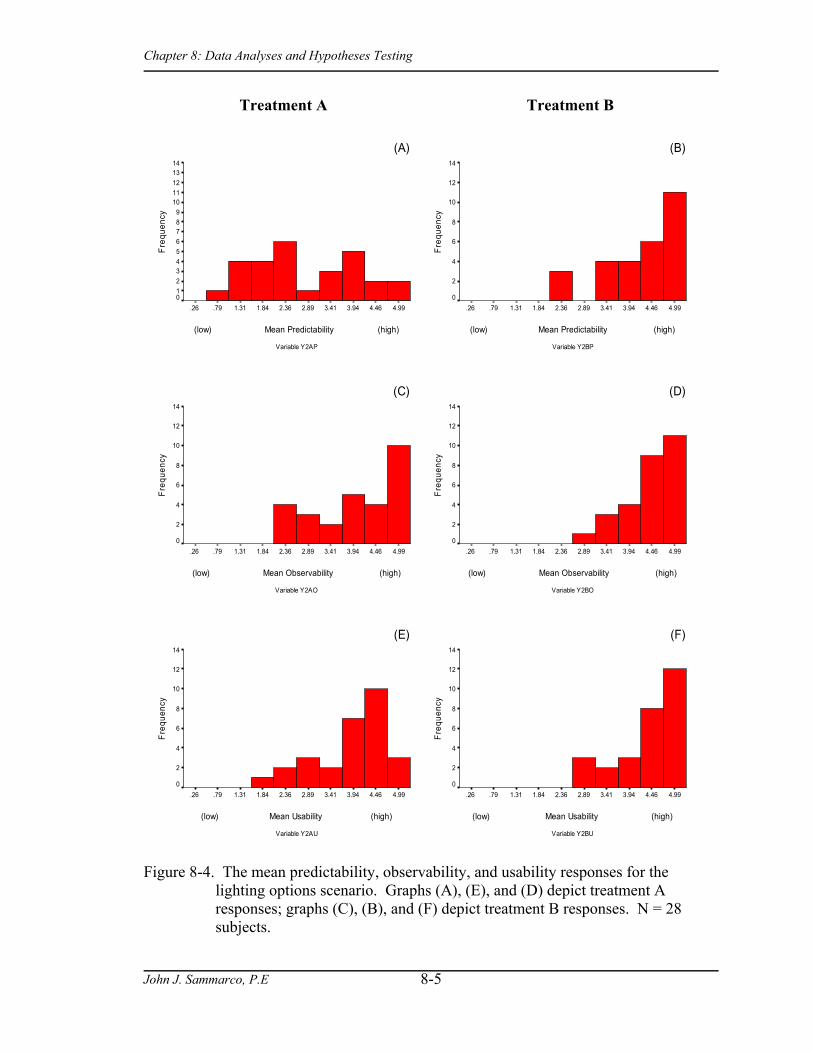
Chapter 8: Data Analyses and Hypotheses Testing
John J. Sammarco, P.E
8-5
Treatment A Treatment B
(low) Mean Predictability (high)
4.994.463.943.412.892.361.841.31.79.26
(A)
Variable Y2AP
Freq
uenc
y14131211109876543210
(low) Mean Predictability (high)
4.994.463.943.412.892.361.841.31.79.26
(B)
Variable Y2BP
Freq
uenc
y
14
12
10
8
6
4
2
0
(low) Mean Observability (high)
4.994.463.943.412.892.361.841.31.79.26
(C)
Variable Y2AO
Freq
uenc
y
14
12
10
8
6
4
2
0
(low) Mean Observability (high)
4.994.463.943.412.892.361.841.31.79.26
(D)
Variable Y2BO
Freq
uenc
y
14
12
10
8
6
4
2
0
(low) Mean Usability (high)
4.994.463.943.412.892.361.841.31.79.26
(E)
Variable Y2AU
Freq
uenc
y
14
12
10
8
6
4
2
0
(low) Mean Usability (high)
4.994.463.943.412.892.361.841.31.79.26
(F)
Variable Y2BU
Freq
uenc
y
14
12
10
8
6
4
2
0
Figure 8-4. The mean predictability, observability, and usability responses for the
lighting options scenario. Graphs (A), (E), and (D) depict treatment A responses; graphs (C), (B), and (F) depict treatment B responses. N = 28 subjects.
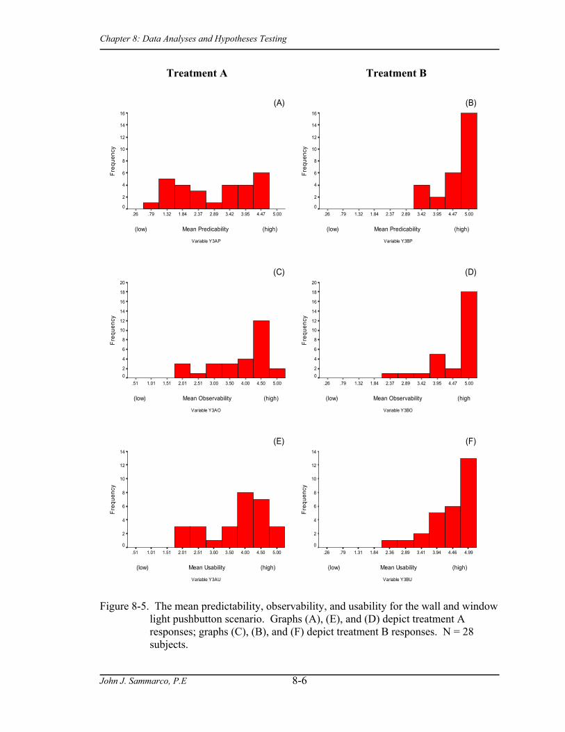
Chapter 8: Data Analyses and Hypotheses Testing
John J. Sammarco, P.E
8-6
Treatment A Treatment B
(low) Mean Predicability (high)
5.004.473.953.422.892.371.841.32.79.26
(A)
Variable Y3AP
Freq
uenc
y16
14
12
10
8
6
4
2
0
(low) Mean Predicability (high)
5.004.473.953.422.892.371.841.32.79.26
(B)
Variable Y3BP
Freq
uenc
y
16
14
12
10
8
6
4
2
0
(low) Mean Observability (high)
5.004.504.003.503.002.512.011.511.01.51
(C)
Variable Y3AO
Freq
uenc
y
20
18
16
14
12
10
8
6
4
20
(low) Mean Observability (high
5.004.473.953.422.892.371.841.32.79.26
(D)
Variable Y3BO
Freq
uenc
y
20
18
16
14
12
10
8
6
4
20
(low) Mean Usability (high)
5.004.504.003.503.002.512.011.511.01.51
(E)
Variable Y3AU
Freq
uenc
y
14
12
10
8
6
4
2
0
(low) Mean Usability (high)
4.994.463.943.412.892.361.841.31.79.26
(F)
Variable Y3BU
Freq
uenc
y
14
12
10
8
6
4
2
0
Figure 8-5. The mean predictability, observability, and usability for the wall and window
light pushbutton scenario. Graphs (A), (E), and (D) depict treatment A responses; graphs (C), (B), and (F) depict treatment B responses. N = 28 subjects.

Chapter 8: Data Analyses and Hypotheses Testing
John J. Sammarco, P.E
8-7
In general, the treatment B histograms for predictability, observability, and
usability are skewed to the right more than the histograms for treatment A. This indicates
treatment B was perceived as having better predictability, observability, and usability
than treatment A.
Table 8-1 lists the median and mode subject responses for predictability,
observability, and usability for treatment A and B. Observations of these values leads us
to infer treatment B was more predictable, observable, and usable because the median
and mode values for treatment B all greater than treatment A with only one exception; the
mode values are equal for observablility of the lighting option treatments.
Table 8-1. Mean and mode of each dependent variable.
Vacant light scene treatments
Lighting options
treatments
Wall and window light pushbutton
treatments
A B A B A B Predictability median
2.42
4.38
2.5
4.67
2.64
4.95
Predictability mode 3.0 5.0 2.5 5.0 4.67 5.0 Observability median
3.79
4.38
3.99
4.6
4.14
5.0
Observability mode 3.86 4.0 5.0 5.0 4.71 5.0 Usability median
3.75
4.67
4.0
4.5
4.04
4.25
Usability mode 4.25 5.0 4.0 5.0 4.5 5.0
Analysis of Internal Validity Threats
All subjects answered all questions of the questionnaire (Appendix D) each time
they completed a scenario The questionnaire data was checked for internal validity to
identify invalid data, to assess data reliability, and to evaluate learning effects and subject
fatigue effects.

Chapter 8: Data Analyses and Hypotheses Testing
John J. Sammarco, P.E
8-8
Outlier Data
Data from two subjects receiving treatment A and two subjects receiving treatment
B were determined to be outliers by using three criteria. First, subject data sets having
unusually high values were identified. Next, those data sets were compared to the
observer’s data to identify major discrepancies. For instance, observer data indicated
subject frustration and confusion; however, the subject data indicated the opposite.
Data Reliability
Cronbach’s Alpha is widely used to estimate data reliability when data are items in
a scale; our data is of a five-point Likert scale. The calculated Cronbach’s alpha is a
reliability coefficient estimate of the data consistency or repeatability given the scale.
Chronbach’s Alpha values range from 0 to 1; a value of .70 or higher is a typical
acceptability benchmark. This was exceeded with Cronbach’s Alpha value of .811.
Data Confounding
The subject responses for each dependent variable and treatment are generalized
and depicted by line graphs of Figures 8-6 and 8-7. These graphs allow inspection of
data trends with respect to the time progression for each scenario as ordered by
treatments A and B. The data, as presented in this form, are useful for determining if
there might be any confounding from learning effects and subject fatigue. A positive-
sloped trend could be an indication that subjects are learning more as time progresses so,
they would rate dependent variables with a higher value. A negative-sloped trend could
be an indication of subject fatiguing as time increases, so they would rate dependent
variables with a lower value. The interpretations of these graphs are given in chapter 9.
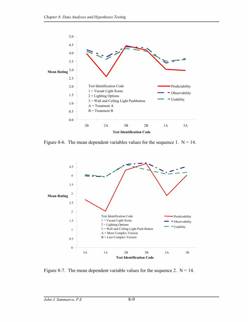
Chapter 8: Data Analyses and Hypotheses Testing
John J. Sammarco, P.E
8-9
Figure 8-6. The mean dependent variables values for the sequence 1. N = 14.
Figure 8-7. The mean dependent variable values for the sequence 2. N = 14.
0
0.5
1
1.5
2
2.5
3
3.5
4
4.5
3A 1A 2B 3B 2A 1B Test Identification Code
Mean Rating
Predictability Observability Usability
Test Identification Code1 = Vacant Light Scene2 = Lighting Options3 = Wall and Ceiling Light Push ButtonA = More Complex VersionB + Less Complex Version
0.0
0.5
1.0
1.5
2.0
2.5
3.0
3.5
4.0
4.5
5.0
1B 2A 3B 2B 1A 3A Test Identification Code
Mean Rating
Predictability Observability Usability
Test Identification Code1 = Vacant Light Scene2 = Lighting Options3 = Wall and Ceiling Light PushbuttonA = Treatment AB = Treatment B

Chapter 8: Data Analyses and Hypotheses Testing
John J. Sammarco, P.E
8-10
Hypothesis Testing
Hypotheses 1 through 3 testing used canonical correlation analysis (CCA) was and
structure correlations were used to determine linear relationships between the
independent and dependent variables. Hypotheses 4 through 6 testing used a one-tailed
Wilcoxon signed ranks test to determine the sign and magnitude of differences between
treatments A and B. Statistical significance measures for hypotheses tests 1 through 3
was determined by using estimates, via boot-strap re-sampling, of the 95% confidence
interval and standard errors. The statistical significance measure for hypotheses tests
four through six was determined by using 1-tailed p-values.
Table 8-2 summarizes the hypotheses and the associated statistical methods and
statistical significance measures. Subsequent sections detail the inferential statistics.
Table 8-2. Summary of hypotheses and the associated statistical tests. Hypothesis & Objective Statistical method
and technique Statistical significance measures
Comments
Hypotheses 1 to 3 Explore relationships between the independent and dependent variables
Canonical correlation analysis (CCA) and structure correlations
Standard error 95% confidence level
- Distribution unknown - Multiple independent variables - Small sample size - Same subjects - Interval & ratio-scaled data
Hypotheses 4 to 6 Test the hypotheses by comparing the directional difference between dependent variables of LCS treatment A (more complex) and treatment B (less complex).
Wilcoxon signed ranks test (one-tailed)
α = .05
- Distribution unknown - Small sample size - Related groups - Same subjects - Interval-scaled data

Chapter 8: Data Analyses and Hypotheses Testing
John J. Sammarco, P.E
8-11
Canonical Correlation Analysis
Canonical correlation analysis (CCA) is one of many multivariate analysis
techniques. Other multivariate techniques include multiple regression analyses,
multivariate analysis of variance (MANOVA), principle component analysis (PCA), and
factor analysis. Each technique has a specific purpose, strengths, weaknesses, and a set
of underlying assumptions concerning the type and distribution of data.
CCA was selected for this research because the variables are distinctively and
logically grouped as independent and dependent variables as described in chapter 5.
CCA is used to identify multiple correlations between sets of the independent and
dependent variables. This is in contrast to using PCA for analyzing a single data set that
does not differentiate between independent and dependent variables. PCA has been
effectively used in prior complexity metrics research. Munsen used PCA to explore 35
complexity metrics and concluded it is realistic to believe that software complexity can
be characterized with just a few variables (Munsen & Khoshgoftaar, 1989). Ammar
(Ammar, Nikzadeh, & Dugan, 1997) also successfully employed PCA for software
complexity metrics.
CCA produces a set of paired canonical variates (a variate is a linear combination
of variables) representing the sets of independent and dependent variables where the
linear combinations are chosen to maximize the correlation. The independent canonical
variate consists of a weighted set of the original independent variable set. The
weightings of the set’s elements are called canonical coefficients. The values of
canonical coefficients determine each element’s contribution to the independent
canonical variate. Likewise, the dependent canonical variable consists of a linear
combination of dependent variables.

Chapter 8: Data Analyses and Hypotheses Testing
John J. Sammarco, P.E
8-12
CCA finds the maximum correlation between the independent and dependent
canonical variates and designates this as the first canonical correlation. This first
correlation explains the most of the relationship correlation between the independent and
dependent canonical variates. The subsequent canonical correlations are ordered in
decreasing values of correlation. They are orthogonal to the first set and have a different
interpretation. The number of canonical correlations is equal to the number of variables
of the smaller set. In this research, the dependent variable set contains three elements; so,
only three canonical correlations are estimated.
In summary, the canonical correlation results in two canonical variates, which are
linear combinations of elements from the original sets of variables such that a maximum
correlation exists between the two canonical variates. Although the result is useful, it is
desirable to look at structure correlation coefficients that are the Pearson correlation
coefficients between the canonical variates and the original variables.
Canonical Correlation Analysis Process
The canonical correlation analysis involved multiple analyses steps to complete
tests of hypotheses 1 through 3. The process steps are summarized:
1. Dependent variable correlation analysis 2. Initial correlation analysis to identify highly correlated independent variables; 3. Canonical correlation analysis to determine structure correlations; 4. Bootstrap resample the data to obtain the standard error and to estimate the 95%
confidence interval Step 1: Dependent variable correlation analysis
A Spearman rank-order correlation analysis was conducted on the dependent
variables. The Spearman rank-order correlation is a non-parametric test of the strength
and significance of bivariate correlations. Both variables may be ordinal scale. The
spearman method calculates a coefficient rho (rs) as,

Chapter 8: Data Analyses and Hypotheses Testing
John J. Sammarco, P.E
8-13
rs = 1 - NN
d−
∑3
26 (8-1)
where N is the number of observations and d is the difference between each pair of
variable rankings. A perfect positive correlation results in rs = 1 while a perfect negative
correlation results in rs = -1.
The significance level for the Spearman rank-order correlation coefficient statistics
is α = .05. The p-value is used as the test statistic.
Dependent variable correlation analysis results
Table 8-3 depicts the correlation matrix of dependent variables. The results show a
medium to high levels of association between the dependent variables. All correlations
were significant at < .001 level (1-tailed).
Table 8-3. A matrix of Spearman rank-order correlation coefficient statistics to measure the associations between the dependent variables.
Predictability
Observability
Usability
Predictability
Correlation coefficient rsp-value N
1.000 - 168
.638
.000 *** 168
.549
.000 *** 168
Observability
Correlation coefficient rsp-value N
.638
.000 *** 168
1.000 - 168
.792
.000 *** 168
Usability
Correlation coefficient rsp-value N
.549
.000*** 168
.792
.000 *** 168
1.000 - 168
*** Correlation is significant at the .001 level (1-tailed) Step 2: Initial correlation analysis
The original set of independent variables consisted of 15 metrics and are listed in
Appendix G. The purpose of step 2 was to first filter out redundancies in this data set.
This initial step involved conducting canonical correlation analysis for one independent
variable at a time to the set of dependent variables. The results are listed in Table 8-4.

Chapter 8: Data Analyses and Hypotheses Testing
John J. Sammarco, P.E
8-14
The five highest correlations are in bold. This set of independent variables {X13, X7, X5,
X2, X6} was used in step 3 that determined the structure correlation coefficients.
Table 8-4. Independent variable correlations to a vector of the three dependent variables. The independent variables with the five highest correlations are in bold.
Independent Variable
Description Correlation
X13 Critical-vertex input cyclomatic complexity 0.354 X7 Critical-state out-degree 0.209 X5 Critical-state changes 0.208 X2 Output cyclomatic complexity 0.195 X6 Critical-state in-degree 0.181 X4 Graph degree 0.139 X14 Critical-vertex output cyclomatic complexity 0.137 X8 Critical-state cyclomatic complexity 0.132 X3 All paths 0.120 X15 Critical-vertex unique conditions 0.116 X9 Critical-state Sheppard complexity 0.180 X12 Critical-vertex Sheppard complexity 0.101 X10 Critical-vertex in-degree 0.092 X11 Critical-vertex out-degree 0.090 X1 Cyclomatic complexity 0.754
Step 3: Structure Correlation
The raw canonical coefficients can be difficult to interpret. Structure correlations
are very useful to facilitate their interpretations (Cliff, 1987; Shafto, Degani, & Kirlik,
2003; Degani, 1996). Structure correlations are derived from the raw canonical
coefficients and represent the Pearson correlation of each original variable to the
canonical variate.
The structure correlations for the first pair of canonical variates are graphically
depicted by Figure 8-8 to emphasis the negative correlation between the dependent and
independent variates. Table 8-5 lists the structure correlation values. These were the
final results.

Chapter 8: Data Analyses and Hypotheses Testing
John J. Sammarco, P.E
8-15
X13
X3 X2 X6
Predictability Observability
Usability
X7
-1.2
-1
-0.8
-0.6
-0.4
-0.2
0
0.2
0.4
0.6
0.8
Str
uctu
re C
orre
latio
n
Figure 8-8. A graphical depiction of structure correlations for the first pair of canonical
variates. Note the negative correlation between the canonical variates
Table 8-5. Structure correlation values for the first pair of canonical variates. Dependent Independent Variables
Structure correlation
√ Predictability (p) -0.993 √ Observability (o) -0.585 √ Usability (u) -0.455 √ X13 0.542 √ X7 0.316 √ X3 0.315 √ X2 0.294 √ X6 0.272
Step 4: Bootstrap Re-sampling
The bootstrap re-sampling method (Efron & Tibshirani, 1993) was used to obtain
the estimates of standard error estimate and the 95% confidence limit for the structure
correlations. The reason for using bootstrap is that we have no formula for the standard
error of a complicated statistic such as the structure correlation.
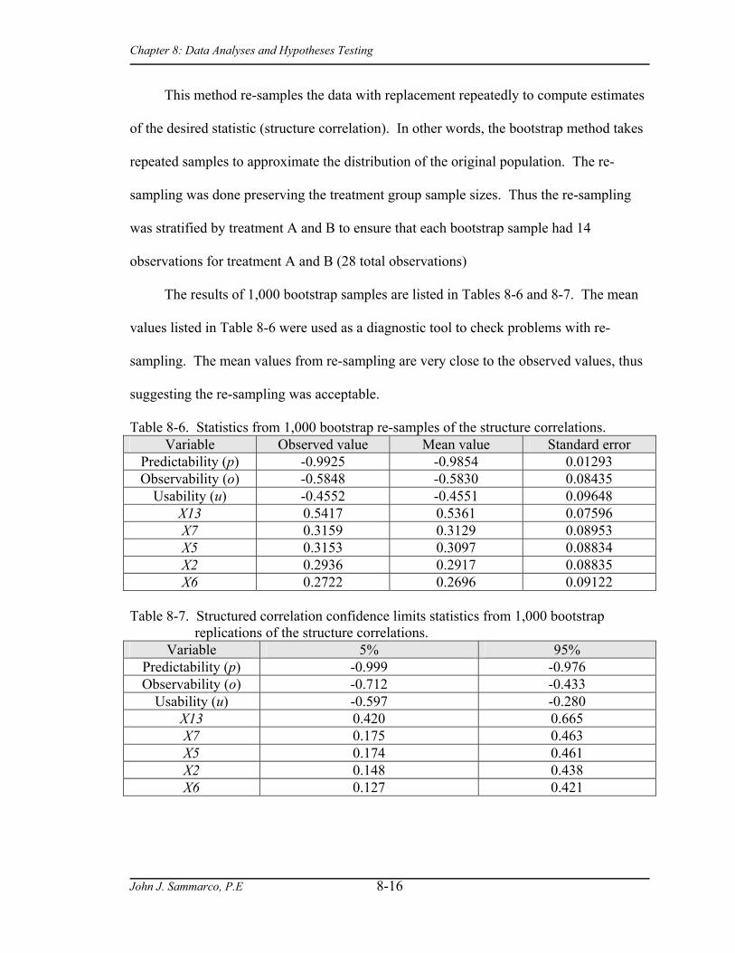
Chapter 8: Data Analyses and Hypotheses Testing
John J. Sammarco, P.E
8-16
This method re-samples the data with replacement repeatedly to compute estimates
of the desired statistic (structure correlation). In other words, the bootstrap method takes
repeated samples to approximate the distribution of the original population. The re-
sampling was done preserving the treatment group sample sizes. Thus the re-sampling
was stratified by treatment A and B to ensure that each bootstrap sample had 14
observations for treatment A and B (28 total observations)
The results of 1,000 bootstrap samples are listed in Tables 8-6 and 8-7. The mean
values listed in Table 8-6 were used as a diagnostic tool to check problems with re-
sampling. The mean values from re-sampling are very close to the observed values, thus
suggesting the re-sampling was acceptable.
Table 8-6. Statistics from 1,000 bootstrap re-samples of the structure correlations. Variable Observed value Mean value Standard error
Predictability (p) -0.9925 -0.9854 0.01293 Observability (o) -0.5848 -0.5830 0.08435
Usability (u) -0.4552 -0.4551 0.09648 X13 0.5417 0.5361 0.07596 X7 0.3159 0.3129 0.08953 X5 0.3153 0.3097 0.08834 X2 0.2936 0.2917 0.08835 X6 0.2722 0.2696 0.09122
Table 8-7. Structured correlation confidence limits statistics from 1,000 bootstrap
replications of the structure correlations. Variable 5% 95%
Predictability (p) -0.999 -0.976 Observability (o) -0.712 -0.433
Usability (u) -0.597 -0.280 X13 0.420 0.665 X7 0.175 0.463 X5 0.174 0.461 X2 0.148 0.438 X6 0.127 0.421

Chapter 8: Data Analyses and Hypotheses Testing
John J. Sammarco, P.E
8-17
Wilcoxon Signed Rank Test
The Wilcoxon signed-rank test (Hollander & Wolfe , 1973) is a nonparametric
statistical significance test of the equality of central tendency (median) for two related
samples of interval scale. It is used to test the direction and magnitude of difference
between a related pair of samples. The Wilcoxon signed rank is calculated as follows,
assuming no ties in the data groups:
( ) ( )( )T R
n n n n n= −
+−
÷
+ +
2
12
12
1 2 124 (8-2)
where
T = test statistic;
R2 = ranked sum of negative data group differences;
n = number of nonzero data group differences;
If there are ties in the data groups, the Wilcoxon signed rank test is calculated as follows:
( ) ( )( )T R
n n n n n t ti i
i
g
= −+
−
÷
+ +−
−
=∑2
3
1
12
12
1 2 124 2 (8-3)
where
ti = number of differences of equal absolute values in the ith tied group;
g = number of tied data groups;
If T > Z1-α/2 then reject Ho, else accept Ho. The p-value is calculated by
ρ = 2 x [1-Φ(T)] (8-4)
Z is a standard normal (Gaussian) random variate (with mean 0 and variance 1)
and Phi is the standard normal cumulative distribution function.
The related pair of samples has a significant difference if the calculated value of T
is equal or less than the critical Wilcoxon’s T value. The software program SPSS, used
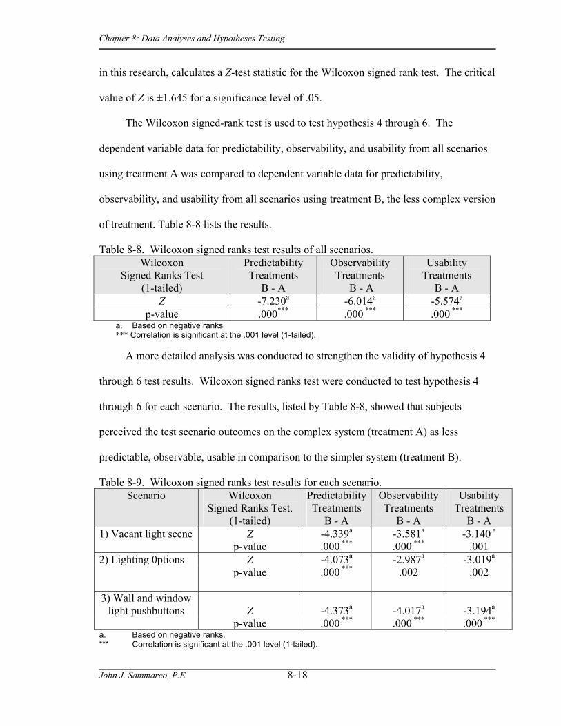
Chapter 8: Data Analyses and Hypotheses Testing
John J. Sammarco, P.E
8-18
in this research, calculates a Z-test statistic for the Wilcoxon signed rank test. The critical
value of Z is ±1.645 for a significance level of .05.
The Wilcoxon signed-rank test is used to test hypothesis 4 through 6. The
dependent variable data for predictability, observability, and usability from all scenarios
using treatment A was compared to dependent variable data for predictability,
observability, and usability from all scenarios using treatment B, the less complex version
of treatment. Table 8-8 lists the results.
Table 8-8. Wilcoxon signed ranks test results of all scenarios. Wilcoxon
Signed Ranks Test (1-tailed)
Predictability Treatments
B - A
Observability Treatments
B - A
Usability Treatments
B - A Z -7.230a -6.014a -5.574a
p-value .000*** .000 *** .000 *** a. Based on negative ranks *** Correlation is significant at the .001 level (1-tailed).
A more detailed analysis was conducted to strengthen the validity of hypothesis 4
through 6 test results. Wilcoxon signed ranks test were conducted to test hypothesis 4
through 6 for each scenario. The results, listed by Table 8-8, showed that subjects
perceived the test scenario outcomes on the complex system (treatment A) as less
predictable, observable, usable in comparison to the simpler system (treatment B).
Table 8-9. Wilcoxon signed ranks test results for each scenario. Scenario Wilcoxon
Signed Ranks Test. (1-tailed)
PredictabilityTreatments
B - A
Observability Treatments
B - A
Usability Treatments
B - A 1) Vacant light scene Z -4.339a -3.581a -3.140 a p-value .000 *** .000 *** .001 2) Lighting 0ptions Z -4.073a -2.987a -3.019a
p-value .000 *** .002 .002
3) Wall and window light pushbuttons
Z
-4.373a
-4.017a
-3.194a
p-value .000 *** .000 *** .000 *** a. Based on negative ranks. *** Correlation is significant at the .001 level (1-tailed).

Chapter 8: Data Analyses and Hypotheses Testing
John J. Sammarco, P.E
8-19
Summary
Descriptive statistics were presented to describe the subject characteristics data and
subject response data for warm-up tests and the scenario tests. Next, an internal validity
threat analysis was conducted to target invalid data, data reliability, and data confounding
from learning effect and subject fatigue. The results do not show significant internal
validity threats from these sources. Hypotheses testing commenced once data validity
was verified.
Canonical correlation analysis and structure correlations were used to test
hypotheses 1 through 3 − the dependent variables predictability, observability, and
usability correlate with our NAT metrics of complexity. The results showed structure
correlations exceeding .25 for five metrics, standard errors of less than .10, and a
statistically significant 95% confidence interval. The five NAT metrics that correlated
with our dependent variables were: X15, the critical-vertex input cyclomatic complexity;
X7, the critical-state out-degree; X5, the number of critical state changes; X2, the output
cyclomatic complexity; X6, the critical state in-degree. A Wilcoxon signed ranks test
was used to test hypotheses 4 through 6 and the results were also statistically significant.
The results showed that subjects perceived the test scenario outcomes of the complex
system (treatment A) as less predictable, observable, usable in comparison to the simpler
system (treatment B).
Literature Cited
Ammar, H., Nikzadeh, T., & Dugan, J. (1997). A Methodology for Risk Assessment and Performance Analysis of Large Scale Software Systems. International Conference on Engineering Mathematics and Physics.
Cliff, N. (1987). Analyzing multivariate data. Harcourt Brace Jovanovich.

Chapter 8: Data Analyses and Hypotheses Testing
John J. Sammarco, P.E
8-20
Degani, A. (1996). Modeling Human-Machine Systems: On Modes, Errors, and Patterns of Interaction. Unpublished doctoral dissertation, Georgia Institute of Technology.
Efron, B., & Tibshirani, R. (1993). An Introduction to the Bootstrap. New York: Chapman and Hall.
Hollander, M., & Wolfe, D. A. (1973). Nonparametric statistical inference. New York: John Wiley & Sons.
Munsen, J. C., & Khoshgoftaar, T. M. (1989). The Dimensionality of Program Complexity. Proceedings of the 11th Annual Conference on Software Engineering
Shafto, M. G., Degani, A., & Kirlik, A. Canonical Correlation Analysis of Data on Human-Automation Interaction [Web Page]. URL http://human-factors.arc.nasa.gov/IHpublications/shafto/canonical-corr/canonical-corr.html [2003, October 9].

Chapter 9: Discussion
John J. Sammarco, P.E
9-1
CHAPTER 9 DISCUSSION
This chapter addresses two core questions of this research: Does the data support
the research hypotheses and, what is the meaning and significance of the results.
The acceptance or rejection of each research hypotheses is based on inferences
from two parts: 1) the analysis and interpretation of internal validity threats common to
all hypotheses; 2) the statistical test criteria for acceptance. Following this is a discussion
of the implications, limitations, and future areas of research.
Relevant Data for all Hypotheses
The acceptance or rejection of a research hypothesis based solely on statistical test
criteria results in a weakly supported inference. Potentially, numerous threats to internal
validity can exist so, type I or II errors could result. This section discusses the steps
taken to reduce internal validity threats.
Internal Validity Threats
Each potential threat is listed and discussed as follows:
• Data confounding from the scenario instructions: Subject responses for the dependent variables predictability, observability, and usability could be biased due to subjects having difficulty following and understanding scenario instructions.
This seems unlikely based on the warm-up data for variable W1− the mean value for the subject’s ease of following and understanding the warm-up instructions. Of 28 subjects, 24 rated W1 very favorably with a greater than 3.94 out of a maximum of 5.0. The distribution for W1 had a positive skew to the right (the highest score) as depicted by Figure 9-1(A).
• Data confounding from the GUI: Biased responses for the dependent variables predictability, observability, and usability could be due to subjects having difficulty with the GUI.

Chapter 9: Discussion
John J. Sammarco, P.E
9-2
This seems unlikely based on the warm-up data for variable W2− the mean value for the subject’s ease of using the GUI to run the warm-up. Of 28 subjects, 24 rated W2 greater than 3.58 out of a maximum of 5.0 score. The distribution forW2 had a positive skew to the right (the highest score) as depicted by Figure 9-1(B).
(low) Mean Rating of Warmup (high)
4.994.463.943.412.892.361.841.31.79.26
(A)
Variable W1
Freq
uenc
y
14
12
10
8
6
4
2
0
(low) Mean Rating of GUI (high)
5.234.684.133.583.032.481.931.38.83.28
(B)
Variable W2
Freq
uenc
y
14
12
10
8
6
4
2
0
Figure 9-1. Mean subject responses for the warm-up session. Graph (A) depicts the ease
following and understanding the warm-up instructions. Graph (B) depicts the GUIs ease of use.
• Invalid data: Data from four subjects was eliminated because of consistent strings of high ratings and because this data was inconsistent with observer’s data. For instance, out of 36 questions, 34 were rated 5.0 and two questions near the end of the questionnaire were rated 4.0.
• Data reliability: The data reliability was accepted given Cronbach’s Alpha = .811. An alpha of .70 or higher is a typical benchmark of acceptability.
• Learning effects or subject fatigue: From inspection of data trends, one can infer learning effects and fatigue. A positive-sloped trend could be an indication that subjects are learning more as time progresses so, they would rate dependent variables with a higher value. A negative-sloped trend could be an indication of subject fatiguing as time increases, so they would rate dependent variables with a lower value. The data trends of Figures 9-2 and 9-3 were used to infer data confounding from learning effects or fatigue for treatments A or B. We failed to detect trends indicating data confounding.
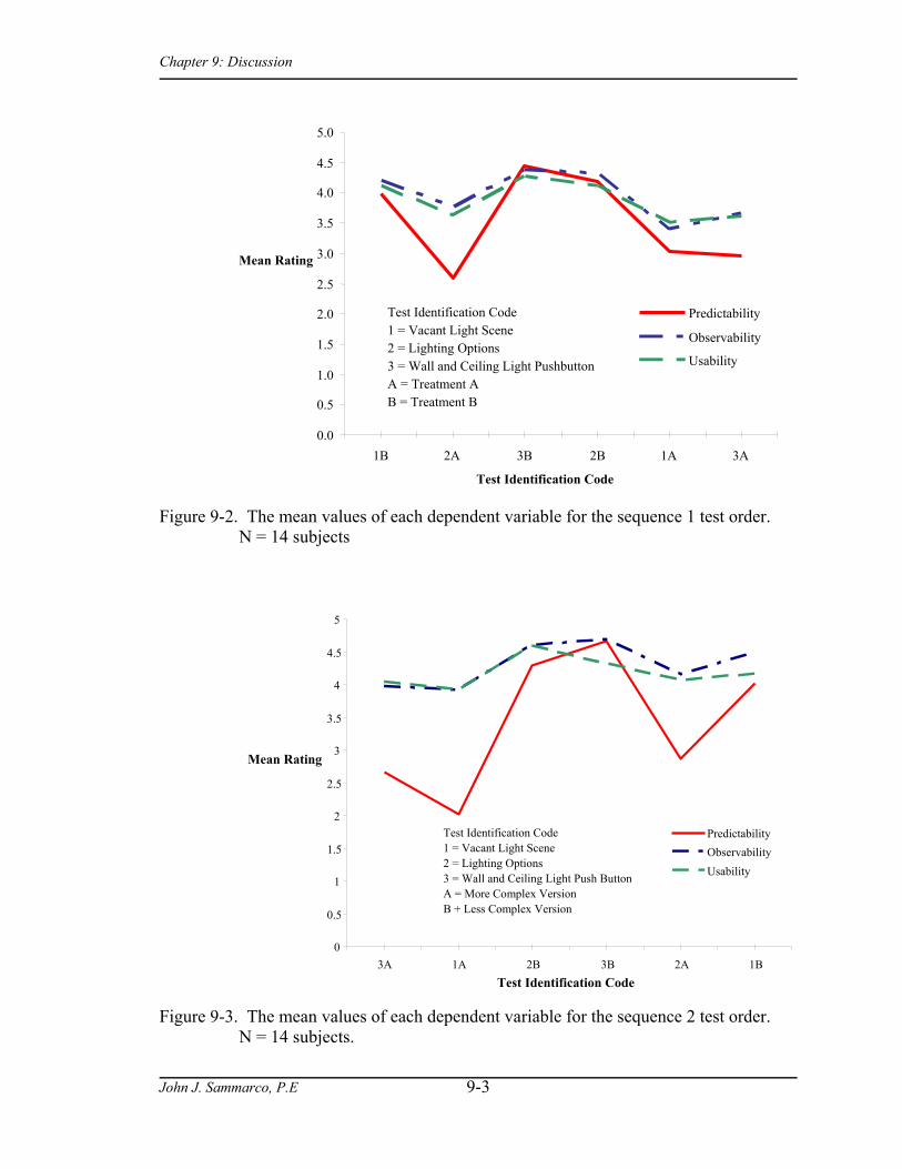
Chapter 9: Discussion
John J. Sammarco, P.E
9-3
Figure 9-2. The mean values of each dependent variable for the sequence 1 test order.
N = 14 subjects
Figure 9-3. The mean values of each dependent variable for the sequence 2 test order.
N = 14 subjects.
0
0.5
1
1.5
2
2.5
3
3.5
4
4.5
5
3A 1A 2B 3B 2A 1BTest Identification Code
Mean Rating
PredictabilityObservabilityUsability
Test Identification Code1 = Vacant Light Scene2 = Lighting Options3 = Wall and Ceiling Light Push ButtonA = More Complex VersionB + Less Complex Version
0.0
0.5
1.0
1.5
2.0
2.5
3.0
3.5
4.0
4.5
5.0
1B 2A 3B 2B 1A 3A
Test Identification Code
Mean Rating
Predictability
Observability
Usability
Test Identification Code1 = Vacant Light Scene2 = Lighting Options3 = Wall and Ceiling Light PushbuttonA = Treatment AB = Treatment B

Chapter 9: Discussion
John J. Sammarco, P.E
9-4
Hypotheses 1 Through 3
The first three research hypothesis concern the existence of correlations between
subject perceptions of the system (the dependent variables of predictability, observability,
and usability) and NAT metrics of system complexity (the independent variables).
Fifteen NAT metrics of system complexity comprised the set of independent variables.
The hypotheses are summarized as follows:
Hypothesis 1:
H0: There is not a correlation between NAT metrics and system predictability.
H1: NAT metrics are correlated to system predictability.
Hypothesis 2:
H0: There is not a correlation between NAT metrics and system observability.
H1: NAT metrics are correlated to system observability.
Hypothesis 3:
H0: There is not a correlation between NAT metrics and system usability.
H1: NAT metrics are correlated to system usability.
Relevant Data
Five out of 15 metrics had a statistically significant structure correlation to the set
of dependent variables as depicted by Table 9-1. The statistical significance was
established from 1,000 bootstrap re-sampling calculations (as previously described in
section “Step 4: Bootstrap Re-sampling” of chapter 8.) for standard error and a 95%
confidence interval.

Chapter 9: Discussion
John J. Sammarco, P.E
9-5
Table 9-1. Structure correlations and statistical significance measures for the first pair of canonical variates.
Independent variables
Structure correlation
Standard error
Confidence limits 5% 95%
X13 0.542 0.07596 0.420 0.665 X7 0.316 0.08953 0.175 0.463 X5 0.315 0.08834 0.174 0.461 X2 0.294 0.08835 0.148 0.438 X6 0.272 0.09122 0.127 0.421
Generally, structure correlations less than .30 are dropped because the contribution
to the canonical variate is minimal (Shafto, Degani, & Kirlik, 2003); This benchmark
was relaxed to .25; hence, the entire set of independent variables {X13, X7, X5, X2, X6}
were included for the first canonical variate. The benchmark was relaxed because this
portion of the research is largely exploratory, and because the information content of the
independent data was limited. as compared to the dependent variable data. The
independent variable data contained only 16 unique values; the dependent variable data
has 168 unique values.
Next, the standard error and confidence interval are calculated for each structure
correlation. A standard error less than .100 is acceptable for exploratory research; all the
standard errors listed in Table 9-1 meet these acceptance criteria. The 95% confidence
limit is exampled as follows:
A confidence interval gives an estimated range of values which is likely to include an unknown population parameter, the estimated range being calculated from a given set of sample data.
If independent samples are taken repeatedly from the same population, and a confidence interval calculated for each sample, then a certain percentage (confidence level) of the intervals will include the unknown population parameter. Confidence intervals are usually calculated so that this percentage is 95% …
Confidence limits are the lower and upper boundaries / values of a confidence interval, that is, the values which define the range of a confidence interval. The

Chapter 9: Discussion
John J. Sammarco, P.E
9-6
upper and lower bounds of a 95% confidence interval are the 95% confidence limits (Easton & McColl, 2003).
None of the confidence intervals in Table 9-1 include zero; therefore, the estimates
of structure correlations confidence levels are statistically significantly different from
zero (alpha = 0.05).
Null Hypotheses Rejection
The null hypothesis was rejected hypothesis 1, 2, and 3. This was based on
hypotheses test results of structure correlations exceeding .25 as shown by Table 9-1,
standard errors of less than .10, confidence intervals that are statistically significant as
shown by Table 9-2, and the steps to reduce internal validity threats.
Hypotheses 4 Through 6
The last three research hypothesis concern the existence of decreasing directional
differences between subject perceptions of LCS treatment A (more complex) and LCS
treatment B (less complex). The hypotheses are summarized as follows:
Hypothesis 4:
H0: Increasing interactive complexity does not decrease system predictability.
H1: Increasing interactive complexity decreases system predictability.
Hypothesis 5:
H0: Increasing interactive complexity does not decrease system observability.
H1: Increasing interactive complexity decreases system observability.
Hypothesis 6:
H0: Increasing interactive complexity does not decrease system usability.
H1: Increasing interactive complexity decreases system usability.

Chapter 9: Discussion
John J. Sammarco, P.E
9-7
Relevant Data
The resulting Wilcoxon signed-ranks test results listed by Table 9-2 show highly
negative differences between the dependent variables of treatments A and B. This means
the median of the population distribution from treatment A was less than the median of
the population distribution from treatment A; simply, treatment A was more complex
than treatment B. Secondly, the differences between treatment medians are very highly
statistically significant with p-values less than 0.001 (one-tailed). P-values are explained
as follows:
The probability value (p-value) of a statistical hypothesis test is the probability of getting a value of the test statistic as extreme as or more extreme than that observed by chance alone, if the null hypothesis H0, is true.
It is the probability of wrongly rejecting the null hypothesis if it is in fact true.
It is equal to the significance level of the test for which we would only just reject the null hypothesis. The p-value is compared with the actual significance level of our test and, if it is smaller, the result is significant. That is, if the null hypothesis were to be rejected at the 5% significance level, this would be reported as "p < 0.05".
Small p-values suggest that the null hypothesis is unlikely to be true. The smaller it is, the more convincing is the rejection of the null hypothesis. It indicates the strength of evidence for say, rejecting the null hypothesis H0, rather than simply concluding "Reject H0' or "Do not reject H0" (Easton & McColl, 2003).
Table 9-2. Wilcoxon signed-ranks test results an aggregation of all scenarios. Wilcoxon
Signed-ranks test (1-tailed) Predictability
Treatments B - AObservability
Treatments B - AUsability
Treatments B - AZ -7.230a -6.014a -5.574a
p value .000*** .000 *** .000 *** b. Based on negative ranks *** Statistical significance < .001 (one-tailed)
The results depicted by Table 9-2 indicate that treatments are different with regard
to predictability, observability and usability, and the directional differences indicate that

Chapter 9: Discussion
John J. Sammarco, P.E
9-8
treatment A has the larger median values. Wilcoxon signed-ranks test were conducted to
test hypothesis 4 through 6 for each scenario. The results are listed by Table 9-3.
Table 9-3. Wilcoxon signed-ranks test results for each scenario. Scenario Wilcoxon
Signed-ranks test (1-tailed)
PredictabilityTreatments
B - A
Observability Treatments
B - A
Usability Treatments
B - A Z -4.339a -3.581a -3.140 a 1) Vacant light scene
p value .000 *** .000 *** .001**
Z -4.073a -2.987a -3.019a 2) Lighting 0ptions p value .000 *** .002** .002**
Z -4.373a -4.017a -3.194a 3) Wall and window
light pushbuttons p value .000 *** .000 *** .000 *** a. Based on negative ranks. ** Statistical significance ≤ .01 (one-tailed) *** Statistical significance ≤ .001 (one-tailed)
The results showed a significant directional difference and that treatment A has the
larger median value for each scenario. These are very highly significant statistical
differences with p values less than < .001 (one-tailed) except for observability and
usability for the Lighting options scenario that has a highly significant statistical
difference with a one-tailed p-value of 0.002. The results of this in-depth analysis also
support rejection of the null hypotheses.
Lastly, the hypotheses testing results for research hypotheses 1 through 3 give
added insight. Specifically, the graphical depiction of structure correlations for the first
pair of canonical variates, depicted by Figure 9-4, shows very strong negative structure
correlations for the canonical variate composed of the original dependent variables (note
that a perfect negative correlation is -1); therefore, as the independent variables X13, X7,
X5, X2, and X6 increase, the dependent variables of predictability, observability, and
usability decrease.

Chapter 9: Discussion
John J. Sammarco, P.E
9-9
Figure 9-4. A graphical depiction of structure correlations for the first pair of canonical
variates. Note the negative correlation between the canonical variates.
Null Hypotheses Rejection
The null hypotheses are rejected for research hypothesis 4, 5, and 6. The rejection
was based on the Wilcoxon hypotheses test results of Tables 9-2 and 9-3 showing that
treatment A was perceived by subjects as more complex than treatment B; also, the p-
values of these results exceeded the statistical significance level of 05. Secondly, the
strong negative correlations between independent and dependent structure correlations,
depicted by Figure 9-4, supported the decision to not accept the null hypotheses.
Implications
This research can be used as a practical tool for addressing system-level hazards in
embedded-computer based systems. Specifically, the hazards are those resulting from
NAT complexities. Mitigation of these hazards is very important because computer-
based systems are proliferating in many safety-critical applications and many incidents
have occurred. Over 400 computer-related incidents have been documented (Neumann,
X13
X5 X2 X6
Predictability Observability
Usability
X7
-1
-0.8
-0.6
-0.4
-0.2
0
0.2
0.4
0.6
0.8
Structure Correlation
Chapter 9: Discussion
John J. Sammarco, P.E
9-10
1995). In 1995, about 2000 deaths were determined to be computer-related (MacKenzie,
1994). In the mining sector, 82 computer-related incidents from 1995 to 2001 were
documented (Sammarco, 2003). The mining incidents involved the hazard of unexpected
movement. This is a significant hazard so NIOSH research is addressing this by
developing best practice recommendations and the NAT complexity assessment
methodology of this research (Sammarco, 1999). The existence of this safety issue is
troubling, but more troubling is that our traditional tools do not effectively handle
complexity-related hazards (Leveson, 2000).
This research enables quantification of NAT complexities of system-level
requirements. This enables NAT complexities impacting safety to be identified,
analyzed, and mitigated before they are propagated to subsequent life cycle phases.
Safety is an emergent property of the system so safety must be addressed at the system-
level as done by this research. This is in contrast to other approaches that quantify
attributes of the software subsystem. Obviously, these approaches do not address the
system but they also take place much later in the system life cycle where the software is
already written. Thus, it is more costly to correct.
The implications of this research are discussed in detail through means of a
practical example addressing the important issue of requirements errors.
Requirements Engineering
The vacant light scene scenario, first described in chapter 6, serves to illustrate a
practical engineering application involving an incompletely defined function. The
practicality and importance of this research is strengthened by this illustration because of
the nature of requirements errors; most errors occur in the requirements (Davis, 1993)
(Lutz, 1996); errors are much less costly to correct at the requirements phase than later

Chapter 9: Discussion
John J. Sammarco, P.E
9-11
(Davis, 1993) (Nelson, Clark, & Spurlock, 1999); requirement errors propagate to cause
errors in later life cycle phases (Kelly, Sherif, & Hops, 1992).
Requirement specification errors fall into two categories: errors of omission and
errors of commission. Requirements errors are common. A study of primary causes of
failure for 34 industrial accidents found that 44.1% of the causes were attributed to the
requirements specification (UK Health and Safety Executive, 1995). Similar results were
found for the mining sector (Sammarco, 2003).
Secondly, it is very beneficial to address requirements issues early in the
requirements phase, where most of the errors occur, because it is less costly to correct
them compared to later development stages (Davis, 1993; Jones, 1994).
The vacant light scene scenario provides an example of an error of omission
because the functionality is incompletely specified. The vacant light scene scenario is
now described.
The vacant light scene
The vacant light scene for treatments A and B is summarized by the listings in
Table 9-4. The behaviors for treatments A and B are identical up to the time of five
minutes. At that time, the vacant light scene activates and remains activated for treatment
B (the less complex system). Treatment A differs in that the vacant light scene does not
activate until the subject re-enters the office at seven minutes.
The LCS requirement U4 of section 3.1.1 of the LCS problem description, defines
the behavior for the vacant light scene (Queins et al., 2000). It states:
“If the room is reoccupied after more than T1 minutes after the last person has left the room, the default light scene has to be established.”

Chapter 9: Discussion
John J. Sammarco, P.E
9-12
Both treatments meet the LCS requirements for the vacant light scene because for
treatments A and B, the vacant light scene is “on” when the subject reoccupies the office
after the time delay expired. The requirements defining the vacant light scene operation
are incomplete, thus there is an error of omission.
Table 9-4. Vacant light scene scenario values for treatment A and B. The items of
primary interest are in bold. Time (Minutes)
LCS Mode
Light Scene
Treatment A Vacant Light (Window)
Treatment B Vacant Light (Window)
0 occupied occupied disabled disabled 1 temp. empty occupied disabled disabled 2 temp. empty occupied disabled disabled 3 temp. empty occupied disabled disabled 4 temp. empty occupied disabled disabled 5 (delay time )
temp. empty
vacant
disabled
enabled @ 20 watts
6 temp. empty vacant disabled enabled @ 20 watts 7 occupied vacant enabled @ 20 watts enabled @ 20 watts
The complexity assessment methodology of this research can be used as a tool to
help decide which design, treatment A and B, is less complex. In less complex designs
the end-user is not likely to create a hazardous situation because the system is less
predictable, observable, and useable (the dependent variables of this research).
This research can be used as a tool to help improve system safety early in the
requirements phase where interventions are the most cost-effective.
Limitations
Three primary limitations of this research are listed in order of priority and
discussed. The last two limitations concerning human subjects and external validity are
interrelated.

Chapter 9: Discussion
John J. Sammarco, P.E
9-13
Predictive limitations:
The complexity assessment methodology of this research involves relative
comparisons of systems under development or of existing systems. At this point, it has
limited use as a prediction tool or system. A prediction system is defined to clarify this
limitation:
“A prediction system consists of a mathematical model together with a set of prediction procedures for determining unknown parameters and interpreting results.” (Littlewood, 1989)
This research is useful for relative assessments but it lacks mathematical models
and inference procedures to identify and assign a probability to future outcomes. This
research does not establish benchmarks for the independent variables X13, X7, X5, X2,
and X6. Thus, at this point, one cannot infer with a great degree of certainty that the
value of any independent variable should not exceed a specific benchmark. If the
research did establish these benchmarks, then one could use them to target specific areas
for simplification. Hence, additional research is needed to realize a predictive tool. The
complexity assessment methodology of this research can serve as a solid basis for
predictive research.
Limited subject diversity
The data from our volunteer subject characterizations indicates a relatively
homogenous group of people. The potential exists that subjects had similar perceptions
because of the homogenous makeup of the group. Therefore, this can potentially be a
threat to external validity with respect to generalizations to other populations.
Subject data was collected during pre-test activities. Analysis of subject data
shows that there were very small numbers of people with non-technical backgrounds,

Chapter 9: Discussion
John J. Sammarco, P.E
9-14
people in the 18 to 35-age range, and women. The most predominate characteristics are
as follows:
• 78.1% - technical job classification; • 71.8% - 45-65 years old; • 87.3% - male; • 84.4% - PC experience rated at 4 or 5 (expert).
There is a positive aspect to the sample population limitations. We infer that it was
more difficult to elicit negative subject perceptions of system predictability,
observability, and usability (the dependent variables) because the typical subject had
considerable experience with technical systems and PC’s. This was an advantage
because their mental models of the system most likely included a more complete
structural model of the system because they had researched, designed, and analyzed other
complex, technical systems at NIOSH. Some subjects commented they had figured out
how the more complex LCS (treatment A) was designed.
The dependent variable measurements are based upon user perceptions. Human
perceptions are affected by many factors including age, race, gender, education, and
social factors; hence, perceptions can potentially contain a large degree of variability.
The subjects are a limited sample of the population. This can be a threat to external
validity; however, the years of technical experience could have given the volunteer
subjects an advantage over more generalized sample populations.
External validity
The research is externally valid if it can be generalized to other populations or to
other embedded computer systems. The external validity limitations that could affect
generalization to other populations were addressed. It is not known if the resulting set of

Chapter 9: Discussion
John J. Sammarco, P.E
9-15
independent variables is useful for other systems, or if the same inferences concerning the
six research hypotheses would pertain to other systems.
There is a potential lack of generalization to other systems; however, this is not an
obvious or intrinsic threat to external validity because this research focuses on a
complexity assessment methodology and not the specific results with respect to the
specific metrics comprising the set of independent variables. More importantly, the
methodology can be generalized to other systems. Specifically, the SCR tools have been
successfully used to model a wide variety of complex, real-time embedded systems
including avionics systems, a submarine communications system, and safety-critical
portions of a nuclear power plant (Heitmyer, Jeffords, & Labaw, 1996). Secondly, the
metrics of this research are not specific to a given system but can be determined from any
SCR dependency graph.
More research using other subject samples and systems is needed to verify the
extent of external validity with respect to the specific results. However, it can be stated
that the complexity assessment methodology of this research can be generalized to other
systems and subject populations.
Summary
Canonical correlation analysis and structure correlations were used to test null
hypotheses 1 through 3 −the dependent variables predictability, observability, and
usability do not correlate with our NAT metrics of complexity. The results showed
structure correlations exceeding .25 for five metrics, standard errors of less than .10, and
a statistically significant 95% confidence interval. The five NAT metrics that correlated
with our dependent variables were: X15, critical-vertex input cyclomatic complexity; X7,

Chapter 9: Discussion
John J. Sammarco, P.E
9-16
critical-state out-degree; X5, number of critical state changes; X2, output cyclomatic
complexity; X6, critical state in-degree.
A Wilcoxon signed ranks test was used to test null hypotheses 4 through 6 −
increasing NAT complexity does not decreases system predictability, observability, and
usability. The results showed that subjects perceived the test scenario outcomes of the
complex system (treatment A) as less predictable, observable, usable in comparison to the
simpler system (treatment B).
Based on hypotheses test results and the steps to guard internal validity, the null
hypotheses were rejected for research hypotheses one through six.
Lastly, the primary limitations of this research concern the research’s limited use as
a predictive tool and potential threats to validity because continence subjects were used
and because this research is just one empirical study. More empirical research is needed
to address these limitations.
Literature Cited
Davis, A. (1993). Software Requirements: Objects, Functions, and States. Prentice- Hall.
Easton, V. J., & McColl, J. H. The STEPS Statistics Glossary [Web Page]. URL http://www.stats.gla.ac.uk/steps/glossary/alphabet.html [2003, October 10]. Notes: Version 1.1
Heitmyer, C., Jeffords, R. D., & Labaw, B. G. (1996). Automated Consistency Checking of Requirements Specifications. ACM Transactions on Software Engineering and Methodology, Vol. 5(No. 3), pp. 231-261.
Jones, T. C. (1994). Assessment and Control of Software Risks. Englewood Cliffs, NJ: Prentice Hall.
Kelly, J., Sherif, J., & Hops, J. (1992). An analysis of defect densities found during software inspections. Journal of Systems and Software, Vol 17, pp. 111-117.
Leveson, N. G. (2000). System Safety in Computer-Controlled Automotive Systems. SAE Congress.

Chapter 9: Discussion
John J. Sammarco, P.E
9-17
Littlewood, B. (1989). Predicting software reliability. Philosophical Transactions of the Royal Society of London Vol. 327.
Lutz, R. R. (1996). Targeting Safety-Related Errors During Software Requirements Analysis. The Journal of Systems Software, Vol. 34, pp. 223-230.
MacKenzie, D. (1994). Computer-Related Accidental Death: An Empirical Exploration. Science and Public Policy, Vol. 21, pp. 233-248.
Nelson, M., Clark, J., & Spurlock, M. A. (1999). Curing the Software Requirements and Cost Estimating Blues. pp. 54-60.
Neumann, P. G. (1995). Computer Related RisksThe ACM Press.
Queins, S., Zimmerman, G., Becker, M., Kronengurg, M., Peper, C., Merz, R., & Schafer, J. (2000). The Light Control Case Study: Problem Description. Journal of Universal Computer Science; Special Issue on Requirements Engineering, Vol. 6, No. 7.
Sammarco, J. J. (1999). Safety Framework for Programmable Electronics in Mining. 30-33. Society of Mining Engineers.
Sammarco, J. J. (2003). Addressing the Safety of Programmable Electronic Mining Systems: Lessons Learned. 2002 IEEE Industry Applications Conference.
Shafto, M. G., Degani, A., & Kirlik, A. Canonical Correlation Analysis of Data on Human-Automation Interaction [Web Page]. URL http://human-factors.arc.nasa.gov/IHpublications/shafto/canonical-corr/canonical-corr.html [2003, October 9].
UK Health and Safety Executive. (1995). Her Majesty’s Stationary Office.

Chapter 10: Summary and Conclusions
John J. Sammarco, P.E
10-1
CHAPTER 10 SUMMARY AND CONCLUSIONS
Summary of Research
Normal Accident Theory (NAT) explains that complex system accidents are
inevitable because complex systems, such as computer-based systems, are highly
interconnected, highly interactive, and tightly coupled. For example, over 400 computer-
related incidents occurred between 1976 and 1963 (Neumann, 1995). From 1995 to
2001, 11 computer-related mining incidents in the U.S. were reported by the Mine Safety
and Health Administration; from 1995 to 2002, 71 computer-related mining incidents
were reported in Australia (Sammarco, 2003). The National Institute for Occupational
Safety and Health (NIOSH) has recognized the hazards associated with complex
computer-based mining systems; hence, it is developing a complexity assessment
methodology for programmable-electronic mining systems (Sammarco, 2002).
We are ill-equipped to understand and manage these complexities because we have
not had a scientific methodology to identify and quantify the safety-related complexities
of a system. More specifically, NAT has not been operationalized for computer-based
systems. Our research addresses this limitation. Our specific objective was to define
graph-theoretical metrics to measure or indicate specific NAT attributes of complexity in
the system requirements of computer-based systems.
We theorized there are two types of system complexity. The first is internal − the
complexity of a system’s internal structure. The second is external − the unfamiliar,
unplanned, or unexpected system behaviors as viewed by the human interacting with the
Chapter 10: Summary and Conclusions
John J. Sammarco, P.E
10-2
system. External, complex behaviors can be difficult to observe and not immediately
comprehensible by the end-user (Perrow, 1999). We characterized external complexity
with three variables: predictability, observability, and usability the dependent
variables for our research. We characterized internal complexity by modeling a system’s
specified behavior, and quantifying its NAT attributes with multiple graph-theoretical
metrics our independent variables.
The first challenge was to formally model the specified behavior (requirements) of
a computer-based system such that the model enabled direct or indirect measurement of
internal complexity. Twelve criteria were established to help guide the selection of a
modeling method. The Software Cost Reduction (SCR) method was selected and
successfully used to translate system requirements into dependency graph models to
which we could apply our graph-theoretical metrics.
The next challenge was to define multiple, graph-theoretical metrics to measure or
indicate specific NAT attributes. This was accomplished by deduction abstracting the
thirteen attributes of NAT complexity, as conceptualized by Perrow (Perrow, 1999), to a
generalized view of simple (linear) and complex (nonlinear) systems; selecting a subset
of NAT attributes pertaining to system requirements; deriving multiple metrics for the
subset of NAT attributes. As a result, fifteen metrics were proposed.
Next, the light control system (LCS) was selected as research test vehicle because it
represented a complex, real-world system that afforded human-computer interaction. The
LCS was devised by the Fraunhofer Institute for Experimental Software Engineering as a
case study for requirements engineering seminars. With the research test vehicle in
place, we addressed our research methodology.
Chapter 10: Summary and Conclusions
John J. Sammarco, P.E
10-3
The research methodology was based on a cross-over design. We chose a standard
design because its validity was established, and the strengths and weaknesses were well
known. Our methodology included having 32 volunteer subjects run simulations of the
LCS in order for us to obtain dependent variable data. The data were collected from a
questionnaire each subjected answered after running a simulation. Once data were
collected, we conducted an internal validity threat analysis. Significant internal validity
threats were not evident so we prepared the data for hypotheses testing.
Canonical correlation analysis and structure correlations were used to test null
hypotheses 1 through 3 − the dependent variables predictability, observability, and
usability do not correlate with our NAT metrics of complexity. The results showed
structure correlations exceeding .25 for five metrics, standard errors of less than .10, and
a statistically significant 95% confidence interval. The five NAT metrics that correlated
with our dependent variables were: X15, critical-vertex input cyclomatic complexity; X7,
critical-state out-degree; X5, number of critical state changes; X2, output cyclomatic
complexity; X6, critical state in-degree. A Wilcoxon signed ranks test was used to test
null hypotheses 4 through 6 − increasing NAT complexity does not decrease system
predictability, observability, and usability. The results showed that subjects perceived the
test scenario outcomes of the complex system (treatment A) as less predictable,
observable, usable in comparison to the simpler system (treatment B). Based on
hypotheses test results and the steps to guard internal validity, the null hypotheses were
rejected for research hypotheses one through six as summarized by Table 10-1.

Chapter 10: Summary and Conclusions
John J. Sammarco, P.E
10-4
Table 10-1. A summary of the research hypotheses and associated rejection criteria Null Hypothesis H0 Do not
Reject H0 Reject H0
Rejection criteria
1) There is not a correlation between NAT metrics and system predictability.
X
2) There is not a correlation between NAT metrics and system observability.
X
3) There is not a correlation between NAT metrics and system usability.
X
Structure correlation ≥ .250 Standard error ≤.100 95% Confidence interval does not cross zero
4) Increasing interactive complexity does not decrease system predictability
X
5) Increasing interactive complexity does not decrease system observability
X
6) Increasing interactive complexity does not decrease system usability
X
Wilcoxon sign-ranks test Z ≤ -1.645 p value ≤ .05
We reflect on the implications of this research. Our research quantified NAT
complexities of system-level requirements. This enables an early assessment of NAT
complexities impacting safety before they are propagated to other life cycle phases. Our
research can be used as a requirements engineering tool to compare NAT complexity
impacts from various system requirements. Armed with this knowledge, one can target
requirements to simplify, and measure their simplification efforts.
In subsequent sections, we draw a number of conclusions about the research;
identify the research limitations, and the opportunities for future research.
Conclusions
Several conclusions emerge from this research; these conclusions are based on data
and what was observed and learned. We conclude that this work is a promising and
significant step in meeting our research objective: to operationalize NAT for the system-
level requirements of safety-related computer systems. Several other conclusions are
drawn with respect to the four specific aims of the research, and lastly, it was concluded

Chapter 10: Summary and Conclusions
John J. Sammarco, P.E
10-5
that this research has several limitations and that there are opportunities for future
research.
Conclusion 1
The research objective was partially realized. We qualify this claim as partial
because the research was limited to one system and 32 test subjects; more empirical
research is needed to validate the findings. Nonetheless, we have carried out the first
steps to take NAT from theory to practice. Two arguments support this claim. First,
there was a statistically significant, negative correlation between five NAT metrics of
complexity and the externally visible system attributes of predictability, observability,
and usability. Secondly, we realized each of the specific aims for operationalizing NAT
with respect to the research objective.
• Specific Aim 1: Identify the NAT attributes to operationalize with respect to system requirements.
We conclude we have addressed this aim. We used a process of deduction that enabled us to ascertain that three of 13 NAT attributes can be observed in SCR dependency models of system requirements. Our premise was that NAT attributes could be generalized to linearity where complex systems are nonlinear; simple systems are linear. From this premise, our reasoning led us to identify three NAT attributes to operationalize: interconnectivity, common-mode connections, and multiple control parameters.
• Specific Aim 2: Identify a formal modeling method for system requirements that will afford quantification of the potential metrics.
We conclude the SCR models and simulations successfully served our research needs so, this aim was satisfied. We have shown that the formal system model created with the SCR tool is useful for modeling, simulating, and analyzing human-computer interactions in the context of NAT. The SCR dependency graphs accommodated multiple levels of system abstraction and multiple projections needed for specific aim 3. Secondly, the SCR toolset successfully supported simulation of our model. A PC-based GUI for the simulation was created using SCR simulation tools. Volunteer subjects were able to quickly learn (in about 10 minutes) to run the simulation and effectively understand the simulation such that useful data were collected.

Chapter 10: Summary and Conclusions
John J. Sammarco, P.E
10-6
• Specific Aim 3: Identify potential metrics for each NAT attribute to be operationalized. At least one metric, and ideally four metrics, should be identified for each of these NAT attributes.
We conclude that this aim was satisfied as evidenced by 15 metrics proposed to measure or indicate the three NAT attributes from specific aim 1. We infer a degree of validity to the proposed metrics because our selection process addressed the limitations of NAT and of other metric research, and our selection process addressed the multidimensional aspects of complexity. We used multiple system abstractions and multiple perspectives to obtain our metrics. Three levels of system abstraction formed a hierarchy of SCR dependency graphs that modeled system requirements in increasing detail. For each abstraction, we applied a projection from the system’s input environment, from the output environment of system behaviors visible to humans interacting with the system, and from a collective projection of all the system’s internal dependencies. This process was an effort to address the multidimensional aspects of complexity.
• Specific Aim 4: Determine which, if any of the potential metrics operationalize the NAT attributes for system requirements.
We conclude this aim was satisfied. This is evidenced by data obtained from hypotheses testing and the steps to reduce internal validity threats. Hypotheses test results showed five out of the 15 proposed metrics had structure correlations exceeding .25, standard errors of less than .10, and statistically significant confidence intervals.
Conclusion 2
We conclude the research is not without limitations; additional research is needed
to address these limitations and to advance our knowledge. This conclusion is based on
four research limitations.
• Predictive limitations: The research did not develop mathematical models and inference procedures to identify and assign a probability to future outcomes. More specifically, this research did not establish benchmarks for the complexity metrics; so one cannot make predictions based solely on the metric values.
• NAT operalization limitations: We have operationalized three NAT attributes: interconnectivity, common-mode connections, and multiple, interacting control parameters. This is a small subset; thus, the research is limited to a narrow segment of the 13 NAT attributes of NAT.
• Limited subject diversity: The data from our volunteer subject characterizations indicates a relatively homogenous group of people. The potential exists that subjects had similar perceptions because of the homogenous makeup of the group.

Chapter 10: Summary and Conclusions
John J. Sammarco, P.E
10-7
Therefore, this can potentially be a threat to external validity with respect to generalizations to other populations.
• Unknown external validity: This section addresses generalization to other systems. The resulting set of independent variables X13, X7, X5, X2, and X6 and the rejection of the null hypotheses were based on statistically significant test results specific to the data set. It is not known if these independent variables are useful for other systems, or if the same inferences concerning the six research hypotheses would pertain to other systems. More empirical research is needed to determine external validity.
Future Work
Predictive system research
The research has limitations for use as a predictive tool or system. Much empirical
research is needed to develop accurate models and inference procedures so that NAT
complexity-related hazards can be identified and predicted. Probabilistic mathematical
models are needed as well as a large body of empirical data.
External validity
Thirty-two volunteer subjects were used in this research. This is a limited group in
terms of the quantity and the homogenous make-up of subjects. Therefore, more
empirical research needed study other populations and other computer-based systems.
NAT attribute completeness
Perrow theorized that accidents are inevitable in complex, tightly coupled
technological systems (Perrow, 1999). He characterized complex systems by describing
thirteen attributes. Our research suggests there attributes missing from Perrow’s list of
thirteen attributes of complex systems. We theorize that multiple modes of system
operation are also a NAT attribute. The hazards associated with complex, multi-mode
systems are documented and research has begun (Degani, 1996; Vakil, 2000; Leveson,
Pinnel, Sandys, Koga, & Reese, 1997) but the research is not in the context of NAT

Chapter 10: Summary and Conclusions
John J. Sammarco, P.E
10-8
complexity. Mode confusion is a hazard of multi-mode systems. Mode confusion is
exhibited by system behaviors similar to those as seen in our research: the systems
become less predictable, observable, and usable to the human.
Concluding Remarks
The major contribution of this work is fundamental to scientific research – to gain
knowledge through the discovery of relationship between the variables of interest.
Specifically, NAT has been advanced by defining and quantifying complexity measures,
and showing their inverse relationship to system predictability, observability, and
usability.
This research has taken the first steps to operationalize NAT for computer-based
systems. We have also identified and discussed research opportunities that could advance
NAT operationalization and the general knowledge base. We trust this research will
stimulate and facilitate future research endeavors.

Chapter 10: Summary and Conclusions
John J. Sammarco, P.E
10-9
Literature Cited
Degani, A. (1996). Modeling Human-Machine Systems: On Modes, Errors, and Patterns of Interaction. Unpublished doctoral dissertation, Georgia Institute of Technology.
Leveson, N. G., Pinnel, L. D., Sandys, S. D., Koga, S., & Reese, J. D. (1997). Analyzing Software Specifications for Mode Confusion Potential. Workshop on Human Error and System Development.
Neumann, P. G. (1995). Computer Related Risks The ACM Press.
Perrow, C. (1999). Normal Accidents: Living with High-Risk Technologies. Princeton, NJ: Princeton University Press.
Sammarco, J. J. (2002). A Complexity Assessment Methodology for Programmable Electronic Mining Systems. The 20th International System Safety Conference.
Sammarco, J. J. (2003). Addressing the Safety of Programmable Electronic Mining Systems: Lessons Learned. 2002 IEEE Industry Applications Conference.
Vakil, S. S. Analysis of Complexity Evolution Management and Human Performance Issues in Commercial Aircraft Automation Systems. Unpublished doctoral dissertation, Massachusetts Institute of Technology, Massachusetts Institute of Technology.
Appendix A: Light Control System: Problem Description
APPENDIX A LIGHT CONTROL SYSTEM: PROBLEM DESCRIPTION
The Light Control System: Problem Description (Queins et al., 2000) is reprinted
with the permissions of the authors and Professor Hermann Maurer, Editor-in-Chief of
the Journal of Universal Computer Science.
Literature Cited
Queins, S., Zimmerman, G., Becker, M., Kronengurg, M., Peper, C., Merz, R., & Schafer, J. (2000). The Light Control Case Study: Problem Description. Journal of Universal Computer Science; Special Issue on Requirements Engineering, Vol. 6, No. 7.
John J. Sammarco, P.E
A-1
The Light Control Case Study:Problem Description
Stefan QueinsGerhard Zimmermann
Martin BeckerMartin Kronenburg
Christian PeperRolf Merz
Jürgen Schäfer
(University of Kaiserslautern, Germany{queins, zimmerma, mbecker, kronburg, peper}@informatik.uni-kl.de,
Abstract: This document contains a range of needs and requirements concerning the constructionof a light control system for a floor of a university building. A description of the building architec-ture and of some pre-installed (light-)hardware is included. This problem description was the com-mon input for all participants of the requirements engineering case study “Light Control”.
Key Words: requirements engineering, building automation, problem description
Introductory NoteThis document gives an informal description of the problem “Light Control System”,that is the subject of the considered case study. It is based on two previous versions thathave been used in the Sonderforschungsbereich 501 “Development of Large Systemswith Generic Methods”, a large project at the Computer Science Department of the Uni-versity of Kaiserslautern. The initial version was created in 1995 by Stefan Queins andGerhard Zimmermann. The second version (reported in [Fe+99]) integrates severalchanges by Martin Becker and Martin Kronenburg. This version was also used in a Dag-stuhl Seminar on “Requirements Capture, Documentation, and Validation” that tookplace in June 1999.
Finally, the version presented here is the result of repeated revisions by Martin Kronen-burg and Christian Peper in agreement with Rolf Merz and Jürgen Schäfer from the Elec-trical Engineering Department of the University of Kaiserslautern, who were acting ascustomers in the light control case study (LCCS). Some additional improvements arebased on input received from Daniel Berry, Vincenzo Gervasi, Julio Leite, and Viniciusda Silva Almendra.
Thus, the basic intention of providing a customer document as the basis for the casestudy has been preserved. The revisions were intended to reduce the need for customerfeedback during the LCCS. Furthermore, to achieve solutions that are better comparable,all interactions between the customer and the participants of the case study have beenpublished on the web [CF99].
The problem description “Light Control” is divided into 4 parts. [Part 1] is a brief intro-duction. [Part 2] describes the architecture of the 4th floor of a university building in Kai-
Journal of Universal Computer Science, vol. 6, no. 7 (2000), 586-596submitted: 3/7/00, accepted: 18/7/00, appeared: 28/7/00 Springer Pub. Co.
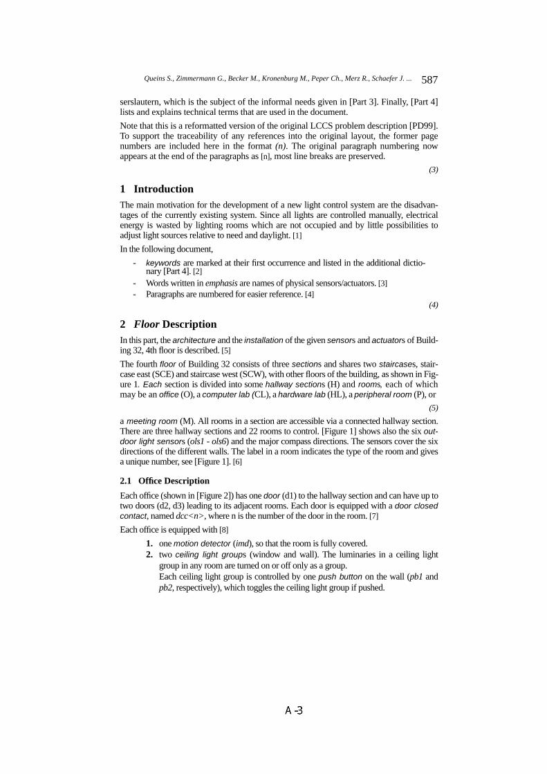
serslautern, which is the subject of the informal needs given in [Part 3]. Finally, [Part 4]lists and explains technical terms that are used in the document.
Note that this is a reformatted version of the original LCCS problem description [PD99].To support the traceability of any references into the original layout, the former pagenumbers are included here in the format (n). The original paragraph numbering nowappears at the end of the paragraphs as [n], most line breaks are preserved.
(3)
1 IntroductionThe main motivation for the development of a new light control system are the disadvan-tages of the currently existing system. Since all lights are controlled manually, electricalenergy is wasted by lighting rooms which are not occupied and by little possibilities toadjust light sources relative to need and daylight. [1]
In the following document,
- keywords are marked at their first occurrence and listed in the additional dictio-nary [Part 4]. [2]
- Words written in emphasis are names of physical sensors/actuators. [3]- Paragraphs are numbered for easier reference. [4]
(4)
2 Floor DescriptionIn this part, the architecture and the installation of the given sensors and actuators of Build-ing 32, 4th floor is described. [5]
The fourth floor of Building 32 consists of three sections and shares two staircases, stair-case east (SCE) and staircase west (SCW), with other floors of the building, as shown in Fig-ure 1. Each section is divided into some hallway sections (H) and rooms, each of whichmay be an office (O), a computer lab (CL), a hardware lab (HL), a peripheral room (P), or
(5)
a meeting room (M). All rooms in a section are accessible via a connected hallway section.There are three hallway sections and 22 rooms to control. [Figure 1] shows also the six out-door light sensors (ols1 - ols6) and the major compass directions. The sensors cover the sixdirections of the different walls. The label in a room indicates the type of the room and givesa unique number, see [Figure 1]. [6]
2.1 Office Description
Each office (shown in [Figure 2]) has one door (d1) to the hallway section and can have up totwo doors (d2, d3) leading to its adjacent rooms. Each door is equipped with a door closedcontact, named dcc<n>, where n is the number of the door in the room. [7]
Each office is equipped with [8]
1. one motion detector (imd), so that the room is fully covered.2. two ceiling light groups (window and wall). The luminaries in a ceiling light
group in any room are turned on or off only as a group.Each ceiling light group is controlled by one push button on the wall (pb1 andpb2, respectively), which toggles the ceiling light group if pushed.
587Queins S., Zimmermann G., Becker M., Kronenburg M., Peper Ch., Merz R., Schaefer J. ...
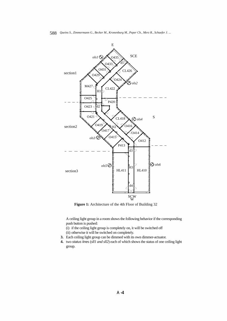
A ceiling light group in a room shows the following behavior if the correspondingpush button is pushed:(i) if the ceiling light group is completely on, it will be switched off(ii) otherwise it will be switched on completely.
3. Each ceiling light group can be dimmed with its own dimmer-actuator.4. two status lines (sll1 and sll2) each of which shows the status of one ceiling light
group.
O435
O433
O431
O429
M427
O425
CL426
O424
CL422
P420
CL418
O416
O423
O421
O419
O417
O415
P413
O414
O412
HL410HL411
ols2
ols3
ols1
ols4
ols6ols5 H3
H2
H1
Figure 1: Architecture of the 4th Floor of Building 32
SCW
S
E
section1
section2
section3
SCE
W
d1
d2
d3
d4
588 Queins S., Zimmermann G., Becker M., Kronenburg M., Peper Ch., Merz R., Schaefer J. ...
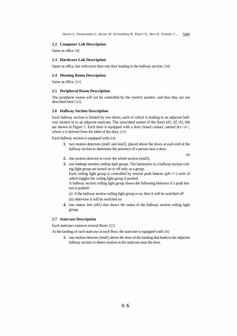
2.2 Computer Lab Description
Same as office. [9]
2.3 Hardware Lab Description
Same as office, but with more than one door leading to the hallway section. [10]
2.4 Meeting Room Description
Same as office. [11]
2.5 Peripheral Room Description
The peripheral rooms will not be controlled by the control system, and thus they are notdescribed here! [12]
2.6 Hallway Section Description
Each hallway section is limited by two doors, each of which is leading to an adjacent hall-way section or to an adjacent staircase. The associated names of the doors (d1, d2, d3, d4)are shown in Figure 1. Each door is equipped with a door closed contact, named dcc<n>,where n is derived from the label of the door. [13]
Each hallway section is equipped with [14]
1. two motion detectors (imd1 and imd2), placed above the doors at each end of thehallway section to determine the presence of a person near a door,
(6)2. one motion detector to cover the whole section (imd3),
3. one hallway section ceiling light group. The luminaries in a hallway section ceil-ing light group are turned on or off only as a group.Each ceiling light group is controlled by several push buttons (pb<i>) each ofwhich toggles the ceiling light group if pushed.A hallway section ceiling light group shows the following behavior if a push but-ton is pushed:
(i) if the hallway section ceiling light group is on, then it will be switched off
(ii) otherwise it will be switched on
4. one status line (sll1) that shows the status of the hallway section ceiling lightgroup.
2.7 Staircase Description
Each staircase connects several floors. [15]
At the landing of each staircase at each floor, the staircase is equipped with [16]
1. one motion detector (imd1) above the door of the landing that leads to the adjacenthallway section to detect motion in the staircase near the door.
589Queins S., Zimmermann G., Becker M., Kronenburg M., Peper Ch., Merz R., Schaefer J. ...
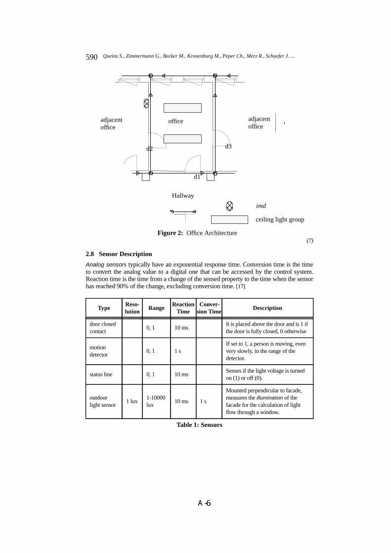
(7)
2.8 Sensor Description
Analog sensors typically have an exponential response time. Conversion time is the timeto convert the analog value to a digital one that can be accessed by the control system.Reaction time is the time from a change of the sensed property to the time when the sensorhas reached 90% of the change, excluding conversion time. [17]
TypeReso-lution
RangeReaction
Time Conver-
sion TimeDescription
door closedcontact
0, 1 10 msIt is placed above the door and is 1 ifthe door is fully closed, 0 otherwise
motiondetector
0, 1 1 sIf set to 1, a person is moving, evenvery slowly, in the range of thedetector.
status line 0, 1 10 msSenses if the light voltage is turnedon (1) or off (0).
outdoorlight sensor
1 lux1-10000lux
10 ms 1 s
Mounted perpendicular to facade,measures the illumination of thefacade for the calculation of lightflow through a window.
Table 1: Sensors
office adjacentoffice
adjacentoffice
imd
d1
d2 d3
Hallway
ceiling light group
Figure 2: Office Architecture
590 Queins S., Zimmermann G., Becker M., Kronenburg M., Peper Ch., Merz R., Schaefer J. ...
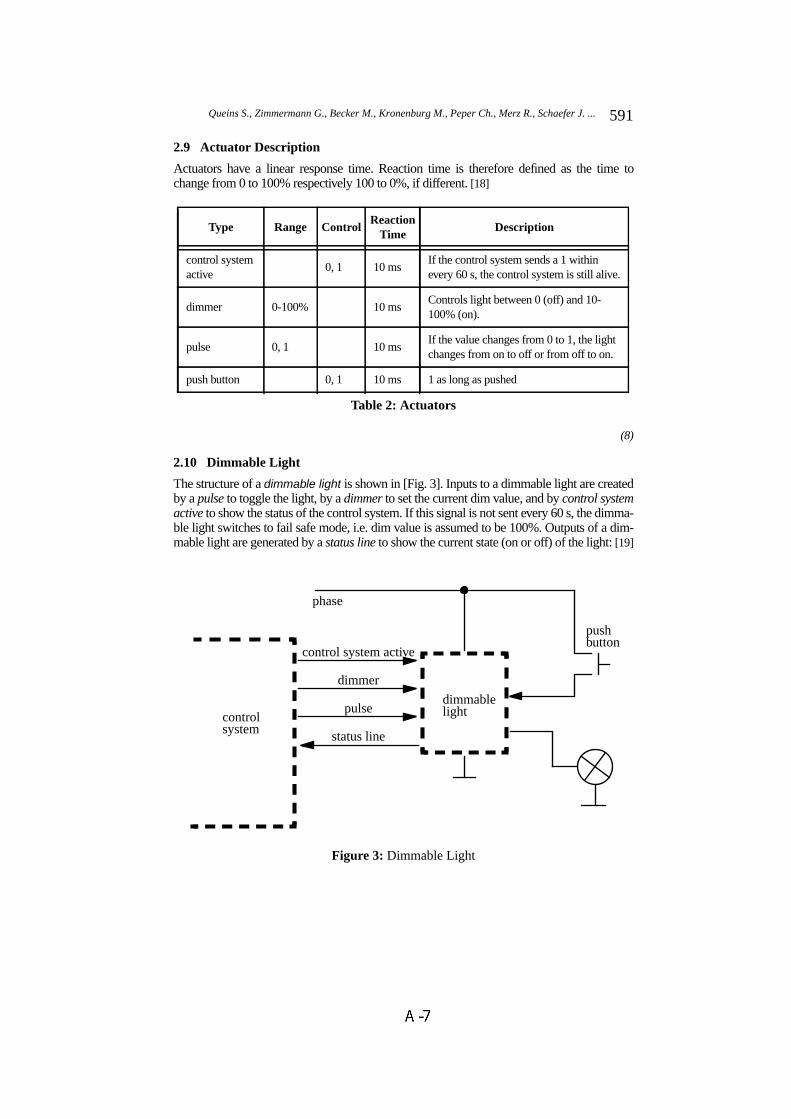
2.9 Actuator Description
Actuators have a linear response time. Reaction time is therefore defined as the time tochange from 0 to 100% respectively 100 to 0%, if different. [18]
(8)
2.10 Dimmable Light
The structure of a dimmable light is shown in [Fig. 3]. Inputs to a dimmable light are createdby a pulse to toggle the light, by a dimmer to set the current dim value, and by control systemactive to show the status of the control system. If this signal is not sent every 60 s, the dimma-ble light switches to fail safe mode, i.e. dim value is assumed to be 100%. Outputs of a dim-mable light are generated by a status line to show the current state (on or off) of the light: [19]
Figure 3: Dimmable Light
Type Range ControlReaction
TimeDescription
control systemactive
0, 1 10 msIf the control system sends a 1 withinevery 60 s, the control system is still alive.
dimmer 0-100% 10 msControls light between 0 (off) and 10-100% (on).
pulse 0, 1 10 msIf the value changes from 0 to 1, the lightchanges from on to off or from off to on.
push button 0, 1 10 ms 1 as long as pushed
Table 2: Actuators
pushbutton
controlsystem
pulse
status line
phase
control system active
dimmable
dimmer
light
591Queins S., Zimmermann G., Becker M., Kronenburg M., Peper Ch., Merz R., Schaefer J. ...

(9)3 Informal NeedsThis part contains the needs for a new light control system for the fourth floor of Building 32of the University of Kaiserslautern. [20]
In [Sec. 3.1], functional needs are listed and in [Sec. 3.2] non-functional needs are listed. [21]
3.1 Functional Needs
The functional needs are split into two groups, user needs and facility manager needs,depending on the person who has expressed them. [22]
3.1.1 User Needs
The user needs are labelled by U<number>. [23]
At first, general user needs are listed, which are demanded for each kind of room: [24]
U1 If a person occupies a room, there has to be safe illumination, if nothing else isdesired by the chosen light scene.
U2 As long as the room is occupied, the chosen light scene has to be maintained.U3 If the room is reoccupied within T1 minutes after the last person has left the room,
the chosen light scene has to be reestablished.U4 If the room is reoccupied after more than T1 minutes since the last person has left
the room, the default light scene has to be established.U5 For each room, the chosen light scene can be set by using the room control panel.U6 For each room, the default light scene can be set by using the room control panel.U7 For each room, the value T1 can be set by using the room control panel.U8 If any outdoor light sensor or the motion detector of a room does not work cor-
rectly, the user of this room has to be informed.U9 The room control panel for an office should contain at least:
(i) a possibility to set each ceiling light group(ii) a possibility to set the chosen and the default light scene(iii)a possibility to set T1
The user needs concerning the offices are: [25]
U10 The ceiling light groups should be maintained by the control system depending onthe current light scene.
U11 A room control panel in an office should be movable as is a telephone.
The user needs for the remaining rooms are: [26]
U12 In all other rooms, the room control panel should be installed near a door leadingto the hallway section.
The user needs for the hallway sections are: [27]
U13 When a hallway section is occupied by a person, there has to be safe illumination.U14 Before a person enters one hallway section from another one or from a staircase,
the hallway section ceiling light group in the section being entered has to be on.
(10)3.1.2 Facility Manager Needs
The facility manager needs are labelled by FM<number>.[28]
FM1 Use daylight to achieve the desired light setting of each room and each hallwaysection whenever possible.
592 Queins S., Zimmermann G., Becker M., Kronenburg M., Peper Ch., Merz R., Schaefer J. ...

FM2 The ceiling light group in each hallway section has to be off when the hallwaysection has been unoccupied for at least T2 minutes.
FM3 The ceiling light groups in a room have to be off when the room is unoccupied forat least T3 minutes.
FM4 For each hallway section, the value T2 can be set by using the facility managercontrol panel.
FM5 For each room, the value T3 can be set by using the facility manager control panel.FM6 The facility manager can turn off the ceiling light groups in a room or hallway
section that is not occupied.FM7 If a malfunction occurs, the facility manager has to be informed.FM8 If a malfunction occurs, the control system supports the facility manager in
finding the reason.FM9 The system provides reports on current and past energy consumption.FM10 All malfunctions and unusual conditions are stored and reported on request.FM11 Malfunctions that the system cannot detect can be entered manually.
3.2 Non-Functional Needs
The non-functional needs are split into several groups according to the aspect they are dealingwith. They are labelled by NF<number>. [29]
3.2.1 Fault Tolerance
In any case of failure, the system shall provide a stepwise degradation of functionality downto manual operability. [30]
Needs in the case of a malfunction of the outdoor light sensor: [31]
NF1 If any outdoor light sensor does not work correctly, the control system for roomsshould behave as if the outdoor light sensor had been submitting the last correctmeasurement of the outdoor light constantly.
NF2 If any outdoor light sensor does not work correctly, the default light scene for allrooms is that all ceiling light groups are on.
NF3 If any outdoor light sensor does not work correctly and a hallway section is occu-pied, the ceiling light group in this hallway section has to be on.
Needs in the case of a malfunction of the motion detector: [32]
NF4 If any motion detector of a room or a hallway section does not work correctly, thecontrol system should behave as if the room or the hallway section were occupied.
Needs in a worst-case failure of the control system: [33]
NF5 If the ceiling light group in a hallway section is controllable neither automaticallynor manually, the ceiling light group of this hallway section has to be on.
3.2.2 Safety and Legal AspectsNF6 All hardware connections are made according to DIN standards.NF7 No hazardous conditions for persons, inventory, or building are allowed.
3.2.3 User InterfaceNF8 The control panels are easy and intuitive to use.NF9 The system issues warnings on unreasonable inputs.
593Queins S., Zimmermann G., Becker M., Kronenburg M., Peper Ch., Merz R., Schaefer J. ...
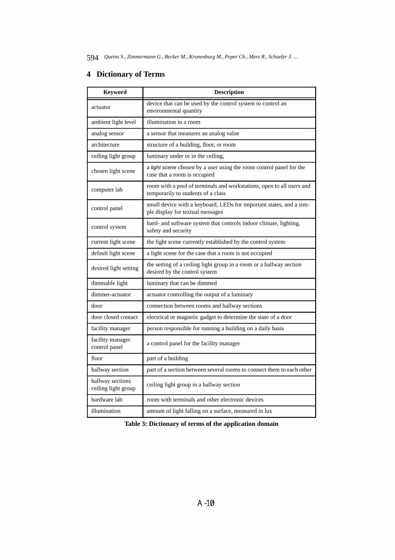
4 Dictionary of Terms
Keyword Description
actuatordevice that can be used by the control system to control anenvironmental quantity
ambient light level illumination in a room
analog sensor a sensor that measures an analog value
architecture structure of a building, floor, or room
ceiling light group luminary under or in the ceiling,
chosen light scenea light scene chosen by a user using the room control panel for thecase that a room is occupied
computer labroom with a pool of terminals and workstations, open to all users andtemporarily to students of a class
control panelsmall device with a keyboard, LEDs for important states, and a sim-ple display for textual messages
control systemhard- and software system that controls indoor climate, lighting,safety and security
current light scene the light scene currently established by the control system
default light scene a light scene for the case that a room is not occupied
desired light settingthe setting of a ceiling light group in a room or a hallway sectiondesired by the control system
dimmable light luminary that can be dimmed
dimmer-actuator actuator controlling the output of a luminary
door connection between rooms and hallway sections
door closed contact electrical or magnetic gadget to determine the state of a door
facility manager person responsible for running a building on a daily basis
facility managercontrol panel
a control panel for the facility manager
floor part of a building
hallway section part of a section between several rooms to connect them to each other
hallway sectionsceiling light group
ceiling light group in a hallway section
hardware lab room with terminals and other electronic devices
illumination amount of light falling on a surface, measured in lux
Table 3: Dictionary of terms of the application domain
594 Queins S., Zimmermann G., Becker M., Kronenburg M., Peper Ch., Merz R., Schaefer J. ...
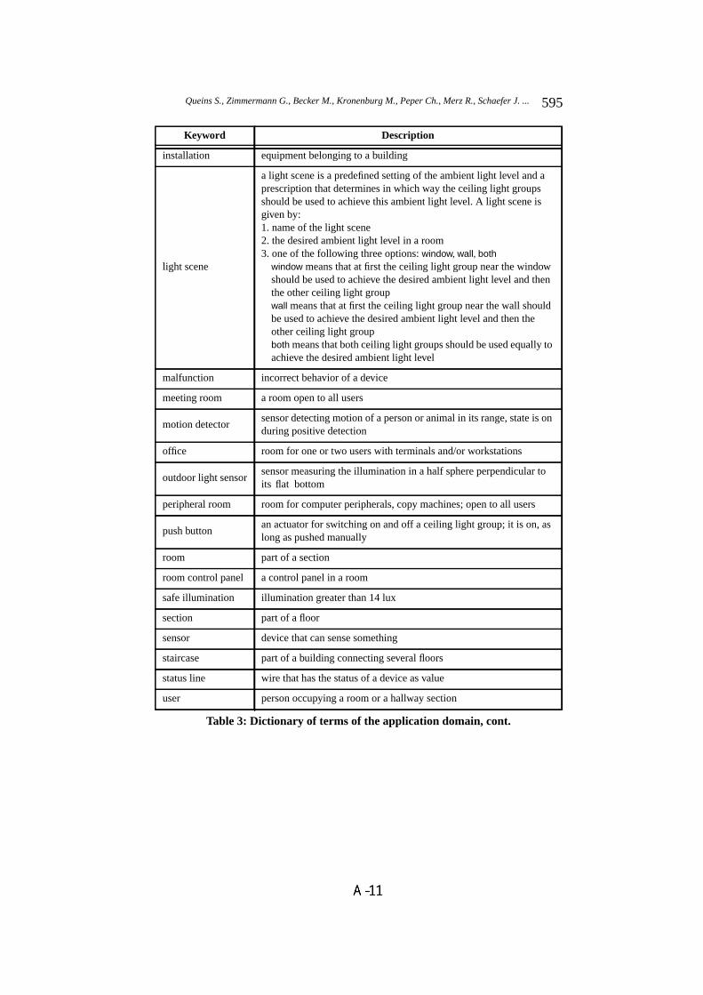
Keyword Description
installation equipment belonging to a building
light scene
a light scene is a predefined setting of the ambient light level and aprescription that determines in which way the ceiling light groupsshould be used to achieve this ambient light level. A light scene isgiven by:1. name of the light scene2. the desired ambient light level in a room3. one of the following three options: window, wall, both
window means that at first the ceiling light group near the windowshould be used to achieve the desired ambient light level and thenthe other ceiling light groupwall means that at first the ceiling light group near the wall shouldbe used to achieve the desired ambient light level and then theother ceiling light groupboth means that both ceiling light groups should be used equally toachieve the desired ambient light level
malfunction incorrect behavior of a device
meeting room a room open to all users
motion detectorsensor detecting motion of a person or animal in its range, state is onduring positive detection
office room for one or two users with terminals and/or workstations
outdoor light sensorsensor measuring the illumination in a half sphere perpendicular toits flat bottom
peripheral room room for computer peripherals, copy machines; open to all users
push buttonan actuator for switching on and off a ceiling light group; it is on, aslong as pushed manually
room part of a section
room control panel a control panel in a room
safe illumination illumination greater than 14 lux
section part of a floor
sensor device that can sense something
staircase part of a building connecting several floors
status line wire that has the status of a device as value
user person occupying a room or a hallway section
Table 3: Dictionary of terms of the application domain, cont.
595Queins S., Zimmermann G., Becker M., Kronenburg M., Peper Ch., Merz R., Schaefer J. ...

References
[Fe+99] R. L. Feldmann, J. Münch, S. Queins, S. Vorwieger, G. Zimmermann:Baselining a Domain-Specific Software Development Process,Technical Report SFB501 TR-02/99, University of Kaiserslautern, 1999
[PD99] The Light Control Case Study: Problem Description, original version athttp://rn.informatik.uni-kl.de/~recs/problem/, University of Kaiserslautern, 1999
[CF99] Customer Feedback of the LCCS, http://rn.informatik.uni-kl.de/~recs/qna/,University of Kaiserslautern, 1999
596 Queins S., Zimmermann G., Becker M., Kronenburg M., Peper Ch., Merz R., Schaefer J. ...

Appendix B: SCR Specification File
John J. Sammarco, P.E
B-1
APPENDIX B SCR SPECIFICATION FILE
Appendix B lists the SCR specifications for treatment B of the wall and window
light pushbutton scenario; this serves as an example of an SCR specification for a given
scenario. SCR specifications were also created for each treatment (A and B) for each of
the three scenarios. This resulted in creating six SCR specifications. The following SCR
specification is based on the file dinreqout.ssl created by the Navel Research Laboratory
(NRL Heitmyer).

Appendix B: SCR Specification File
John J. Sammarco, P.E
B-2
// This is the SCR specification file for the wall and window light pushbutton scenario, treatment B. It is based on the NRL dinreqdout.ssl specification. J. Sammarco identified three specification errors and collaborated with T. Grimm for the corrections. T. Grimm implemented three changes: 1. mIndoorLL made to use the new value of iOLS instead of the old value (a prime was added to the asignement) \ "Light Control Example: mIndoorLL value is set to old iOLS value\" 2. The tNeverOccupied term was added and used in the tCurrentLSOpt and tCurrentLSVal functions to make it properly use the default settings for the first occupant even though the duration result shortly after the initial state is not yet at or beyond mT1 (in other words it assumes the room has been unoccupied starting in the initial state). \"Light Control Example: Duration Initial State Issue\" 3. Add WHEN (NOT iMD) to the end of the second event expression, preventing the error in both cited cases of resetting the room to unoccupied when it really is occupied. \"Light Control Example: Another Duration Initial State Problem plus a Related Problem\" J Sammarco implemented additional changes for the scenario: 1) oWallOuput and oWindowOutput terms created for display purposes. Display = 0 if pulse is off. This reduces confusion because prior version displayed oDimmerWall & oDimmerWindow at some value even though oPulseWall and oPulseWindow were off. 2) Pushbutton behavior changed to behave like traditional dimmer switch Changes to oPulseWall & oPulseWindow"; // This section contains all of the items in the // Type Dictionary. TYPE "yAmbientLevel"; BASETYPE "Integer"; UNITS "n.a."; VALUES "[0,100]"; COMMENT "In %"; TYPE "yLight"; BASETYPE "Enumerated"; UNITS "n.a."; VALUES "off, on"; TYPE "yLightLevel"; BASETYPE "Integer"; UNITS "n.a."; VALUES "[0,10000]"; COMMENT "in lux"; TYPE "yMalfcnLight"; BASETYPE "Enumerated"; UNITS "n.a."; VALUES "green, red"; COMMENT "red indicates a malfunction"; TYPE "yOption"; BASETYPE "Enumerated"; UNITS "n.a."; VALUES "wall, window, both"; COMMENT "Light scene options"; TYPE "yTimer"; BASETYPE "Integer"; UNITS "n.a."; VALUES "[0,30]"; COMMENT "in minutes"; // Mode Class Dictionary.

Appendix B: SCR Specification File
John J. Sammarco, P.E
B-3
MODECLASS "mcStatus"; MODES "unoccupied, occupied,\ntemp_empty"; INITMODE "unoccupied"; // Constant Dictionary. // none // Variable Dictionary. TERM "cMDmalfunction"; TYPE "yMalfcnLight"; INITVAL "green"; ACCURACY "n.a."; TERM "cOLSmalfunction"; TYPE "yMalfcnLight"; INITVAL "green"; ACCURACY "n.a."; TERM "cWallLL"; TYPE "yLightLevel"; INITVAL "0"; ACCURACY "n.a."; TERM "cWallLights"; TYPE "yLight"; INITVAL "off"; ACCURACY "n.a."; TERM "cWindowLL"; TYPE "yLightLevel"; INITVAL "0"; ACCURACY "n.a."; TERM "cWindowLights"; TYPE "yLight"; INITVAL "off"; ACCURACY "n.a."; MON "iChosenLSOpt"; TYPE "yOption"; INITVAL "wall"; ACCURACY "n.a."; MON "iChosenLSVal"; TYPE "yLightLevel"; INITVAL "200"; ACCURACY "n.a."; MON "iDCC"; TYPE "Boolean"; INITVAL "FALSE"; ACCURACY "n.a."; MON "iDefLSOpt"; TYPE "yOption"; INITVAL "wall"; ACCURACY "n.a."; MON "iDefLSVal"; TYPE "yLightLevel"; INITVAL "100"; ACCURACY "n.a."; MON "iFMOverride"; TYPE "Boolean"; INITVAL "FALSE"; ACCURACY "n.a."; MON "iMD"; TYPE "Boolean"; INITVAL "FALSE"; ACCURACY "n.a."; MON "iMDmalfunction"; TYPE "Boolean"; INITVAL "FALSE"; ACCURACY "n.a."; MON "iOLS"; TYPE "yLightLevel"; INITVAL "0"; ACCURACY "n.a."; MON "iOLSmalfunction"; TYPE "Boolean"; INITVAL "FALSE"; ACCURACY "n.a."; MON "iSLLWall"; TYPE "Boolean"; INITVAL "FALSE"; ACCURACY "n.a."; MON "iSLLWindow"; TYPE "Boolean"; INITVAL "FALSE"; ACCURACY "n.a."; MON "iT1"; TYPE "yTimer"; INITVAL "10"; ACCURACY "n.a."; MON "iT3"; TYPE "yTimer"; INITVAL "15"; ACCURACY "n.a."; TERM "mChosenLSOpt"; TYPE "yOption"; INITVAL "wall"; ACCURACY "n.a."; TERM "mChosenLSVal"; TYPE "yLightLevel"; INITVAL "200"; ACCURACY "n.a."; TERM "mDefLSOpt"; TYPE "yOption"; INITVAL "wall"; ACCURACY "n.a."; TERM "mDefLSVal"; TYPE "yLightLevel"; INITVAL "100"; ACCURACY "n.a."; TERM "mFMOverride"; TYPE "Boolean"; INITVAL "FALSE"; ACCURACY "n.a."; TERM "mIndoorLL"; TYPE "yLightLevel"; INITVAL "0";

Appendix B: SCR Specification File
John J. Sammarco, P.E
B-4
ACCURACY "n.a."; TERM "mMDmalfunction"; TYPE "Boolean"; INITVAL "FALSE"; ACCURACY "n.a."; TERM "mOLSmalfunction"; TYPE "Boolean"; INITVAL "FALSE"; ACCURACY "n.a."; TERM "mOccupied"; TYPE "Boolean"; INITVAL "FALSE"; ACCURACY "n.a."; TERM "mT1"; TYPE "yTimer"; INITVAL "10"; ACCURACY "n.a."; TERM "mT3"; TYPE "yTimer"; INITVAL "15"; ACCURACY "n.a."; TERM "mWallLights"; TYPE "yLight"; INITVAL "off"; ACCURACY "n.a."; TERM "mWindowLights"; TYPE "yLight"; INITVAL "off"; ACCURACY "n.a."; CON "oDimmerWall"; TYPE "yAmbientLevel"; INITVAL "0"; ACCURACY "n.a."; CON "oDimmerWindow"; TYPE "yAmbientLevel"; INITVAL "0"; ACCURACY "n.a."; CON "oMDmalfunction"; TYPE "Boolean"; INITVAL "FALSE"; ACCURACY "n.a."; CON "oOLSmalfunction"; TYPE "Boolean"; INITVAL "FALSE"; ACCURACY "n.a."; CON "oPulseWall"; TYPE "Boolean"; INITVAL "FALSE"; ACCURACY "n.a."; CON "oPulseWindow"; TYPE "Boolean"; INITVAL "FALSE"; ACCURACY "n.a."; CON "oWallOutput"; TYPE "yAmbientLevel"; INITVAL "0"; ACCURACY "n.a."; CON "oWindowOutput"; TYPE "yAmbientLevel"; INITVAL "0"; ACCURACY "n.a."; TERM "tCurrentLSOpt"; TYPE "yOption"; INITVAL "wall"; ACCURACY "n.a."; TERM "tCurrentLSVal"; TYPE "yLightLevel"; INITVAL "100"; ACCURACY "n.a."; TERM "tNeverOccupied"; TYPE "Boolean"; INITVAL "TRUE"; TERM "tOverride"; TYPE "Boolean"; INITVAL "FALSE"; ACCURACY "n.a."; TERM "tRemLL"; TYPE "yLightLevel"; INITVAL "0"; ACCURACY "n.a."; MON "time"; TYPE "Integer"; INITVAL "0"; ACCURACY "n.a."; // Assertion Dictionary. // none // Assumption Dictionary. // none // Enumerated Monitored Variable Table. // none // This section contains the event, mode transition, and condition functions. CONDFUNC "cMDmalfunction"; CONDITIONS "NOT mMDmalfunction", "mMDmalfunction"; ASSIGNMENTS "green", "red";

Appendix B: SCR Specification File
John J. Sammarco, P.E
B-5
CONDFUNC "cOLSmalfunction"; CONDITIONS "NOT mOLSmalfunction", "mOLSmalfunction"; ASSIGNMENTS "green", "red"; CONDFUNC "cWallLL"; CONDITIONS "tCurrentLSOpt = both", "tCurrentLSOpt = wall AND tRemLL > 5000", "tCurrentLSOpt = wall AND tRemLL <= 5000", "tCurrentLSOpt = window AND tRemLL > 5000", "tCurrentLSOpt = window AND tRemLL <= 5000"; ASSIGNMENTS "tRemLL / 2", "5000", "tRemLL", "tRemLL - 5000", "0"; EVENTFUNC "cWallLights"; EVENTS "@T(mWallLights = on) WHEN (cWallLights = off) OR @T(mcStatus = occupied)", "@T(mWallLights = off) WHEN (cWallLights = on) OR @T(mcStatus = unoccupied) OR\n@T(mFMOverride) WHEN (NOT (mcStatus = occupied))"; ASSIGNMENTS "on", "off"; CONDFUNC "cWindowLL"; CONDITIONS "tCurrentLSOpt = both", "tCurrentLSOpt = wall AND tRemLL > 5000", "tCurrentLSOpt = wall AND tRemLL <= 5000", "tCurrentLSOpt = window AND tRemLL > 5000", "tCurrentLSOpt = window AND tRemLL <= 5000"; ASSIGNMENTS "tRemLL / 2", "tRemLL - 5000", "0", "5000", "tRemLL"; EVENTFUNC "cWindowLights"; EVENTS "@T(mWindowLights = on) WHEN (cWindowLights = off) OR @T(mcStatus = occupied)", "@T(mWindowLights = off) WHEN (cWindowLights = on) OR @T(mcStatus = unoccupied) OR @T(mFMOverride) WHEN (NOT (mcStatus = occupied))"; ASSIGNMENTS "on", "off"; CONDFUNC "mChosenLSOpt"; CONDITIONS "true"; ASSIGNMENTS "iChosenLSOpt"; CONDFUNC "mChosenLSVal"; CONDITIONS "true"; ASSIGNMENTS "iChosenLSVal"; CONDFUNC "mDefLSOpt"; CONDITIONS "NOT iOLSmalfunction", "iOLSmalfunction"; ASSIGNMENTS "iDefLSOpt", "both"; CONDFUNC "mDefLSVal"; CONDITIONS "NOT iOLSmalfunction", "iOLSmalfunction"; ASSIGNMENTS "iDefLSVal", "10000"; CONDFUNC "mFMOverride"; CONDITIONS "true"; ASSIGNMENTS "iFMOverride";

Appendix B: SCR Specification File
John J. Sammarco, P.E
B-6
EVENTFUNC "mIndoorLL"; EVENTS "@C(iOLS) WHEN (NOT iOLSmalfunction)"; ASSIGNMENTS "iOLS'"; DESCRIPTION "NOTE: This should be a function of iOLS, but we cannot denote functions!!!"; CONDFUNC "mMDmalfunction"; CONDITIONS "true"; ASSIGNMENTS "iMDmalfunction"; CONDFUNC "mOLSmalfunction"; CONDITIONS "true"; ASSIGNMENTS "iOLSmalfunction"; EVENTFUNC "mOccupied"; EVENTS "@T(iMD) OR @T(iMDmalfunction)", "@F(iMD) when ((NOT iDCC OR (duration(iDCC AND iMD) < 1))\nAND NOT iMDmalfunction) OR @T(duration(NOT iMDmalfunction) >= 2)\n WHEN (NOT iMD)"; ASSIGNMENTS "true", "false"; CONDFUNC "mT1"; CONDITIONS "true"; ASSIGNMENTS "iT1"; CONDFUNC "mT3"; CONDITIONS "true"; ASSIGNMENTS "iT3"; CONDFUNC "mWallLights"; CONDITIONS "iSLLWall", "NOT iSLLWall"; ASSIGNMENTS "on", "off"; CONDFUNC "mWindowLights"; CONDITIONS "iSLLWindow", "NOT iSLLWindow"; ASSIGNMENTS "on", "off"; MODETRANS "mcStatus"; FROM "unoccupied" EVENT "@T(mOccupied)" TO "occupied"; FROM "occupied" EVENT "@F(mOccupied)" TO "temp_empty"; FROM "temp_empty" EVENT "@T(duration(NOT mOccupied) > mT3)" TO "unoccupied"; FROM "temp_empty" EVENT "@T(mOccupied)" TO "occupied"; CONDFUNC "oDimmerWall"; CONDITIONS "TRUE"; ASSIGNMENTS "cWallLL/50"; CONDFUNC "oDimmerWindow"; CONDITIONS "true"; ASSIGNMENTS "cWindowLL/50"; CONDFUNC "oMDmalfunction"; CONDITIONS "cMDmalfunction = green", "cMDmalfunction = red"; ASSIGNMENTS "false", "true"; CONDFUNC "oOLSmalfunction";

Appendix B: SCR Specification File
John J. Sammarco, P.E
B-7
CONDITIONS "cOLSmalfunction = green", "cOLSmalfunction = red"; ASSIGNMENTS "false", "true"; EVENTFUNC "oPulseWall"; EVENTS "@T(cWallLights = on) AND (NOT iSLLWall') OR @T(cWallLights = off) AND iSLLWall'", "@C(iSLLWall) AND (cWallLights' = off) ", "@C(iSLLWall) AND (cWallLights' = on) "; ASSIGNMENTS "true", "true", "false"; EVENTFUNC "oPulseWindow"; EVENTS "@T(cWindowLights = on) AND (NOT iSLLWindow') OR @T(cWindowLights = off) AND iSLLWindow'", "@C(iSLLWindow) AND (cWindowLights' = off) ", "@C(iSLLWindow) AND (cWindowLights' = on) "; ASSIGNMENTS "true", "true", "false"; CONDFUNC "oWallOutput"; CONDITIONS "oPulseWall = true", "oPulseWall = false"; ASSIGNMENTS "oDimmerWall", "0"; CONDFUNC "oWindowOutput"; CONDITIONS "oPulseWindow = true", "oPulseWindow = false"; ASSIGNMENTS "oDimmerWindow", "0"; EVENTFUNC "tCurrentLSOpt"; EVENTS "@T(mcStatus = occupied) when (tNeverOccupied OR\n(duration(not(mcStatus = occupied)) >= mT1))", "@C(mChosenLSOpt)"; ASSIGNMENTS "mDefLSOpt", "mChosenLSOpt'"; EVENTFUNC "tCurrentLSVal"; EVENTS "@T(mcStatus = occupied) when (tNeverOccupied OR\n(duration(NOT(mcStatus = occupied)) >= mT1))", "@C(mChosenLSVal)"; ASSIGNMENTS "mDefLSVal", "mChosenLSVal'"; EVENTFUNC "tNeverOccupied"; EVENTS "@T(mOccupied)"; ASSIGNMENTS "FALSE"; EVENTFUNC "tOverride"; EVENTS "@T(mFMOverride) WHEN (NOT (mcStatus = occupied))", "@T(mcStatus = occupied)"; ASSIGNMENTS "true", "false"; CONDFUNC "tRemLL"; MCLASS "mcStatus"; MODES "unoccupied" CONDITIONS "true", "false"; MODES "occupied" CONDITIONS "mIndoorLL > tCurrentLSVal", "mIndoorLL <= tCurrentLSVal"; MODES "temp_empty" CONDITIONS "tOverride OR mIndoorLL > tCurrentLSVal", "NOT tOverride AND mIndoorLL <= tCurrentLSVal"; ASSIGNMENTS "0", "tCurrentLSVal-mIndoorLL";

Appendix B: SCR Specification File
John J. Sammarco, P.E
B-8
Literature Cited
Heitmeyer, C., & Bharadwaj, R (2000). Applying the SCR Requirements Method to the Light Control Case Study. Journal of Universal Computer Science; Special Issue on Requirements Engineering, Vol. 6, No. 7.

Appendix C: Institutional Review Board Exemption
John J. Sammarco, P.E
C-1
APPENDIX C INSTITUTIONAL REVIEW BOARD EXEMPTION
Chairperson Institute Review Board West Virginia University February 11, 2002 Dear Chairperson: I am requesting Institute Review Board exemption for my experiments using human subjects. These experiments are part of my Ph.D. study "A Complexity Assessment Methodology for Safety-Critical, Embedded Systems". My committee chair and faculty advisor is Dr. Roy Nutter from the department of Computer Science and Electrical Engineering (CSEE). My research involves surveys of subjects. The identity of each subject will not be recorded or revealed; thus, I believe this research belongs to category 5 of the A criteria for exemption from board review. The research includes experiments with subjects from private industry. Subjects will use a PC-based simulation and provide feedback concerning their perceptions of system predictability, complexity, and usability. Attached please find: 1) Application for Exemption 2) Sample subject cover letter Sincerely, John J. Sammarco, PE

Appendix C: Institutional Review Board Exemption
John J. Sammarco, P.E
C-2

Appendix D: Subject Questionnaire
John J. Sammarco, P.E
D-1
APPENDIX D SUBJECT QUESTIONAIRE
The subject questionnaire instrument was used to collect data concerning the
subject, warm-up test, and test scenarios for treatments A and B. The questionnaire
consists of closed-ended questions and open-ended questions. A five-level Likert scale is
used for the closed-ended questions.
Appendix D contains the subject questionnaire for those subjects conducting tests
in the order defined by phase A. The subject questionnaire for the phase B ordering is
not shown, but is identical except that the test scenarios are listed in reverse order.

Appendix D: Subject Questionnaire
John J. Sammarco, P.E
D-2
Subject Questionnaire
The Light Control System (LCS) Study
sequence 1

Appendix D: Subject Questionnaire
John J. Sammarco, P.E
D-3
Part 1: User Profile 1.1 Job Title:
1.2 Age range:
~ 18 - 24
~ 25 - 34
~ 35 - 44
~ 45 - 65+
1.3 Sex:
~ Male
~ Female
1.4 Were you involved in the development of the scenarios?
Yes No
1.5 Rate your knowledge about the light control system.
no knowledge expert
1 2 3 4 5
1.6 Rate your level of experience in using a PC with Windows.
none expert
1 2 3 4 5
Please return to the subject instructions and begin the warm-up scenario.
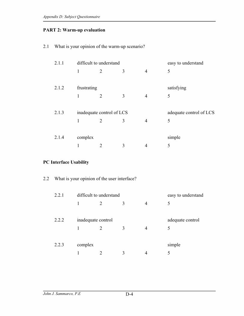
Appendix D: Subject Questionnaire
John J. Sammarco, P.E
D-4
PART 2: Warm-up evaluation
2.1 What is your opinion of the warm-up scenario?
2.1.1 difficult to understand easy to understand
1 2 3 4 5
2.1.2 frustrating satisfying
1 2 3 4 5
2.1.3 inadequate control of LCS adequate control of LCS
1 2 3 4 5
2.1.4 complex simple
1 2 3 4 5
PC Interface Usability
2.2 What is your opinion of the user interface?
2.2.1 difficult to understand easy to understand
1 2 3 4 5
2.2.2 inadequate control adequate control
1 2 3 4 5
2.2.3 complex simple
1 2 3 4 5
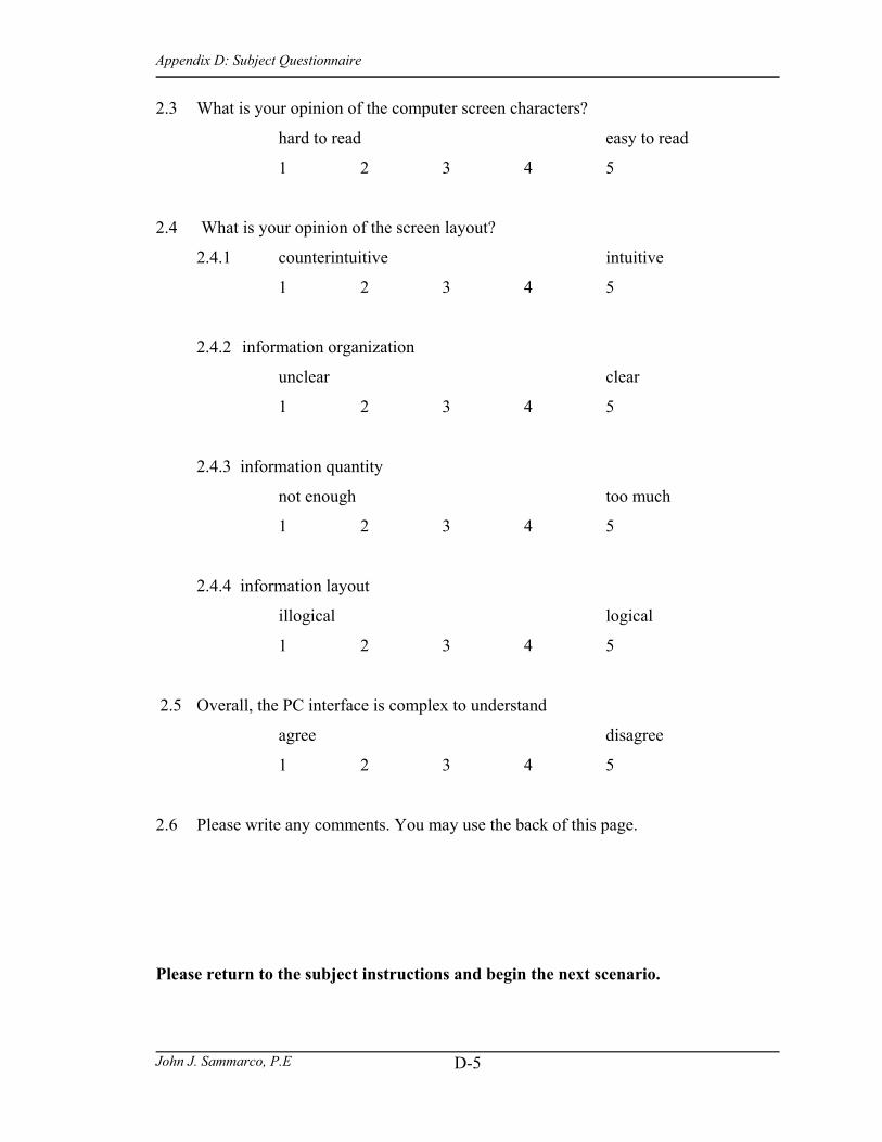
Appendix D: Subject Questionnaire
John J. Sammarco, P.E
D-5
2.3 What is your opinion of the computer screen characters?
hard to read easy to read
1 2 3 4 5
2.4 What is your opinion of the screen layout?
2.4.1 counterintuitive intuitive
1 2 3 4 5
2.4.2 information organization
unclear clear
1 2 3 4 5
2.4.3 information quantity
not enough too much
1 2 3 4 5
2.4.4 information layout
illogical logical
1 2 3 4 5
2.5 Overall, the PC interface is complex to understand
agree disagree
1 2 3 4 5
2.6 Please write any comments. You may use the back of this page.
Please return to the subject instructions and begin the next scenario.

Appendix D: Subject Questionnaire
John J. Sammarco, P.E
D-6
PART 3: Vacant Light Scene
System Predictability
3.1 What is your initial opinion of the system=s behavior?
3.1.1 confusing understandable
1 2 3 4 5
3.1.2 unpredictable predictable
1 2 3 4 5
3.1.3 unstable stable
1 2 3 4 5
3.2 How difficult is anticipating the system=s output or behavior?
difficult easy
1 2 3 4 5
System Observability
3.3 Does the system keep you informed about its status or state?
3.3.1 never always
1 2 3 4 5
3.3.2 inappropriately appropriately
1 2 3 4 5
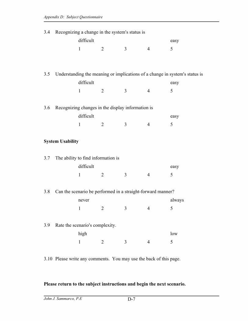
Appendix D: Subject Questionnaire
John J. Sammarco, P.E
D-7
3.4 Recognizing a change in the system=s status is
difficult easy
1 2 3 4 5
3.5 Understanding the meaning or implications of a change in system=s status is
difficult easy
1 2 3 4 5
3.6 Recognizing changes in the display information is
difficult easy
1 2 3 4 5
System Usability
3.7 The ability to find information is
difficult easy
1 2 3 4 5
3.8 Can the scenario be performed in a straight-forward manner?
never always
1 2 3 4 5
3.9 Rate the scenario=s complexity.
high low
1 2 3 4 5
3.10 Please write any comments. You may use the back of this page.
Please return to the subject instructions and begin the next scenario.

Appendix D: Subject Questionnaire
John J. Sammarco, P.E
D-8
PART 4: Lighting Options
System Predictability
4.1 What is your initial opinion of the system=s behavior?
4.1.1 confusing understandable
1 2 3 4 5
4.1.2 unpredictable predictable
1 2 3 4 5
4.1.3 unstable stable
1 2 3 4 5
4.2 How difficult is anticipating the system=s output or behavior?
difficult easy
1 2 3 4 5
System Observability
4.3 Does the system keep you informed about its status or state?
4.3.1 never always
1 2 3 4 5
4.3.2 inappropriately appropriately
1 2 3 4 5
4.4 Recognizing a change in the system=s status is
difficult easy
1 2 3 4 5
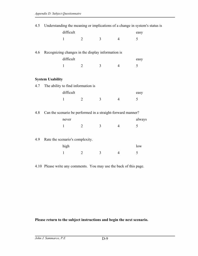
Appendix D: Subject Questionnaire
John J. Sammarco, P.E
D-9
4.5 Understanding the meaning or implications of a change in system=s status is
difficult easy
1 2 3 4 5
4.6 Recognizing changes in the display information is
difficult easy
1 2 3 4 5
System Usability
4.7 The ability to find information is
difficult easy
1 2 3 4 5
4.8 Can the scenario be performed in a straight-forward manner?
never always
1 2 3 4 5
4.9 Rate the scenario=s complexity.
high low
1 2 3 4 5
4.10 Please write any comments. You may use the back of this page.
Please return to the subject instructions and begin the next scenario.
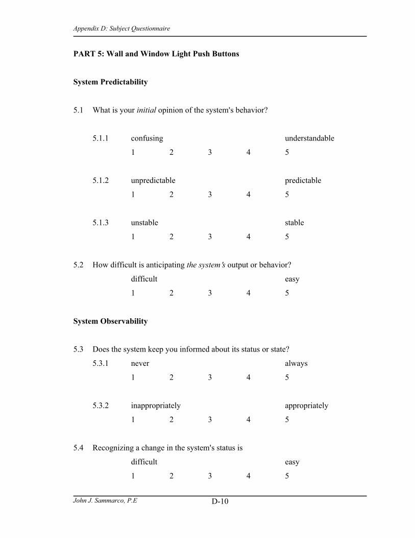
Appendix D: Subject Questionnaire
John J. Sammarco, P.E
D-10
PART 5: Wall and Window Light Push Buttons
System Predictability
5.1 What is your initial opinion of the system=s behavior?
5.1.1 confusing understandable
1 2 3 4 5
5.1.2 unpredictable predictable
1 2 3 4 5
5.1.3 unstable stable
1 2 3 4 5
5.2 How difficult is anticipating the system=s output or behavior?
difficult easy
1 2 3 4 5
System Observability
5.3 Does the system keep you informed about its status or state?
5.3.1 never always
1 2 3 4 5
5.3.2 inappropriately appropriately
1 2 3 4 5
5.4 Recognizing a change in the system=s status is
difficult easy
1 2 3 4 5
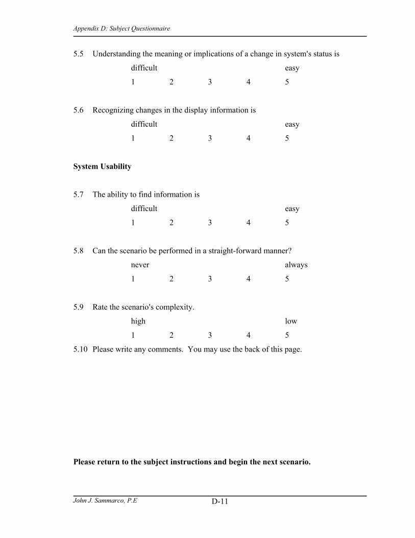
Appendix D: Subject Questionnaire
John J. Sammarco, P.E
D-11
5.5 Understanding the meaning or implications of a change in system=s status is
difficult easy
1 2 3 4 5
5.6 Recognizing changes in the display information is
difficult easy
1 2 3 4 5
System Usability
5.7 The ability to find information is
difficult easy
1 2 3 4 5
5.8 Can the scenario be performed in a straight-forward manner?
never always
1 2 3 4 5
5.9 Rate the scenario=s complexity.
high low
1 2 3 4 5
5.10 Please write any comments. You may use the back of this page.
Please return to the subject instructions and begin the next scenario.

Appendix D: Subject Questionnaire
John J. Sammarco, P.E
D-12
PART 6: Lighting Options
System Predictability
6.1 What is your initial opinion of the system=s behavior?
6.1.1 confusing understandable
1 2 3 4 5
6.1.2 unpredictable predictable
1 2 3 4 5
6.1.3 unstable stable
1 2 3 4 5
6.2 How difficult is anticipating the system=s output or behavior?
difficult easy
1 2 3 4 5
System Observability
6.3 Does the system keep you informed about its status or state?
6.3.1 never always
1 2 3 4 5
6.3.2 inappropriately appropriately
1 2 3 4 5
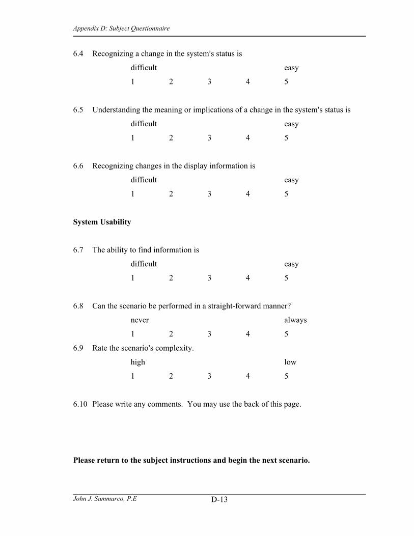
Appendix D: Subject Questionnaire
John J. Sammarco, P.E
D-13
6.4 Recognizing a change in the system=s status is
difficult easy
1 2 3 4 5
6.5 Understanding the meaning or implications of a change in the system=s status is
difficult easy
1 2 3 4 5
6.6 Recognizing changes in the display information is
difficult easy
1 2 3 4 5
System Usability
6.7 The ability to find information is
difficult easy
1 2 3 4 5
6.8 Can the scenario be performed in a straight-forward manner?
never always
1 2 3 4 5
6.9 Rate the scenario=s complexity.
high low
1 2 3 4 5
6.10 Please write any comments. You may use the back of this page.
Please return to the subject instructions and begin the next scenario.

Appendix D: Subject Questionnaire
John J. Sammarco, P.E
D-14
PART 7: Vacant Light Scene
System Predictability
7.1 What is your initial opinion of the system=s behavior?
7.1.1 confusing understandable
1 2 3 4 5
7.1.2 unpredictable predictable
1 2 3 4 5
7.1.3 unstable stable
1 2 3 4 5
7.2 How difficult is anticipating the system=s output or behavior?
difficult easy
1 2 3 4 5
System Observability
7.3 Does the system keep you informed about its status or state?
7.3.1 never always
1 2 3 4 5
7.3.2 inappropriately appropriately
1 2 3 4 5
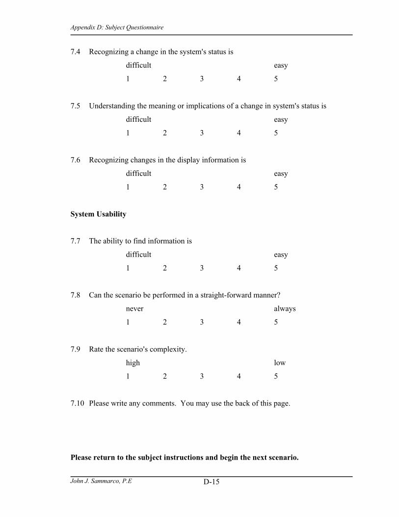
Appendix D: Subject Questionnaire
John J. Sammarco, P.E
D-15
7.4 Recognizing a change in the system=s status is
difficult easy
1 2 3 4 5
7.5 Understanding the meaning or implications of a change in system=s status is
difficult easy
1 2 3 4 5
7.6 Recognizing changes in the display information is
difficult easy
1 2 3 4 5
System Usability
7.7 The ability to find information is
difficult easy
1 2 3 4 5
7.8 Can the scenario be performed in a straight-forward manner?
never always
1 2 3 4 5
7.9 Rate the scenario=s complexity.
high low
1 2 3 4 5
7.10 Please write any comments. You may use the back of this page.
Please return to the subject instructions and begin the next scenario.
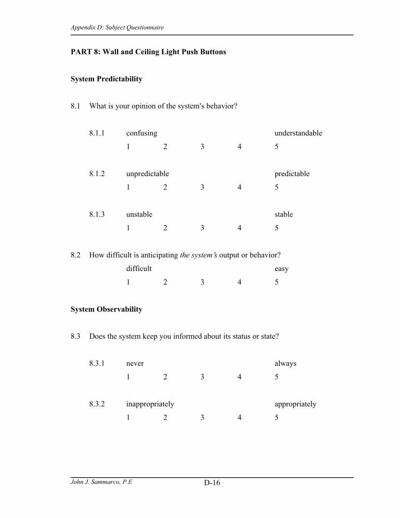
Appendix D: Subject Questionnaire
John J. Sammarco, P.E
D-16
PART 8: Wall and Ceiling Light Push Buttons
System Predictability
8.1 What is your opinion of the system=s behavior?
8.1.1 confusing understandable
1 2 3 4 5
8.1.2 unpredictable predictable
1 2 3 4 5
8.1.3 unstable stable
1 2 3 4 5
8.2 How difficult is anticipating the system=s output or behavior?
difficult easy
1 2 3 4 5
System Observability
8.3 Does the system keep you informed about its status or state?
8.3.1 never always
1 2 3 4 5
8.3.2 inappropriately appropriately
1 2 3 4 5

Appendix D: Subject Questionnaire
John J. Sammarco, P.E
D-17
8.4 Recognizing a change in the system=s status is
difficult easy
1 2 3 4 5
8.5 Understanding the meaning or implications of a change in system=s status is
difficult easy
1 2 3 4 5
8.6 Recognizing changes in the display information is
difficult easy
1 2 3 4 5
System Usability
8.7 The ability to find information is
difficult easy
1 2 3 4 5
8.8 Can the scenario be performed in a straight-forward manner?
never always
1 2 3 4 5
8.9 Rate the scenario=s complexity.
high low
1 2 3 4 5
8.10 Please write any comments. You may use the back of this page.

Appendix D: Subject Questionnaire
John J. Sammarco, P.E
D-18
Part 9: Questionnaire Completion
Please write your comments about any aspect of the questionnaire, or any other
portion of this experiment. Thank you for participating

Appendix E: Subject Instructions
John J. Sammarco, P.E
E-1
APPENDIX E SUBJECT INSTRUCTIONS
Appendix E contains the subject instructions for those subjects conducting tests in
the order defined by phase B. The subject instructions for sequence 1 ordering are not
shown, but are identical except that the test scenarios are in reverse order.

Appendix E: Subject Instructions
John J. Sammarco, P.E E-2
Subject Instructions
The Light Control System (LCS) Study
Sequence 2

Appendix E: Subject Instructions
John J. Sammarco, P.E E-3
Preface
This research is being conducted to fulfill the requirements for my doctoral
dissertation in Computer Engineering in the Department of Computer Science and
Electrical Engineering at West Virginia University. Your participation in this research is
voluntary and your identity will not be documented or disclosed.
The purpose of this research is to learn more about what makes a computer-based
system complex, as perceived by the user.
This portion of the research involves your running six test scenarios on a simulated
computerized office lighting system. Your opinions about the system are given by
answering a questionnaire. Also, an observer will take notes as you operate the system.
To become familiar with the lighting system, you will follow instructions for a
warm-up session. After the warm-up, you follow instructions to run six pre-defined
scenarios for the lighting system. After running each scenario, you are to answer the
questionnaire, take a short break, and then begin the next session until the six scenarios
are completed.
You are encouraged to verbalize your actions, thoughts and opinions during the
experiment.
Thank you for participating.
John J. Sammarco

Appendix E: Subject Instructions
John J. Sammarco, P.E E-4
Experiment Overview
This experiment consists of nine parts. The general process is for you to follow the
instructions, answer the questionnaire, and take a one-minute break. The experiment
takes about 1 hour to complete.
The experiment uses a light control system (LCS), a fictitious system, as a test
vehicle to validate research theories and methodologies. To learn about the LCS you
will:
• Watch a short video about the LCS; • Read a description of the LCS; • Receive “hands-on” training using the LCS in a warm-up session.
Part 1: User Profile
Please answer the user profile questions, part 1 of the questionnaire. Turn to the
next page and read the light control system description once you have completed part 1.

Appendix E: Subject Instructions
John J. Sammarco, P.E E-5
The Light Control System (LCS) Description
The LCS is used to reduce energy costs and help maintain safety. Energy is saved
by automatically reducing lighting intensity when the office is empty for extended
periods, by enabling users to get the light level they need by adjusting a dimmer instead
of using the lights fully on, and by automatically adjusting the lights with respect to
sunlight.
The lighting system controls a light near the window and light near the wall as
depicted by figure 1. Two sensors provide data to the lighting system. A motion sensor
detects if people are in the office; a sunlight sensor measures the office’s natural light.
Figure1 – The office layout for the Light Control System
The LCS controls the office lighting for two lighting scenes: occupied and vacant.
The occupied light scene is used while a person is in the office. The vacant light scene is
used to reduce the lighting when someone leaves the office for an extended period, as set
by a time delay. If the person returns to the office before the time delay expires, the
lighting remains in the occupied light scene. If the person returns after the time delay,
the vacant light scene is enabled and it will be on when re-entering the office. The vacant
and occupied light scenes are controlled with the LCS user-interface panel.
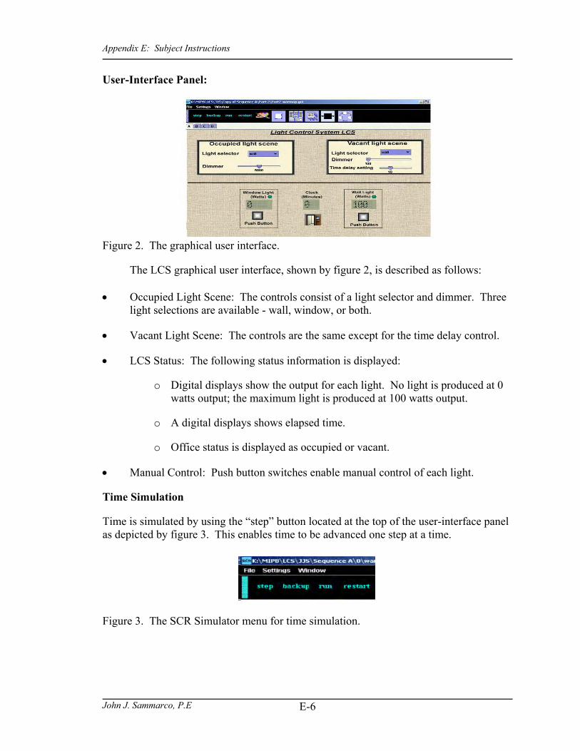
Appendix E: Subject Instructions
John J. Sammarco, P.E E-6
User-Interface Panel:
Figure 2. The graphical user interface.
The LCS graphical user interface, shown by figure 2, is described as follows:
• Occupied Light Scene: The controls consist of a light selector and dimmer. Three light selections are available - wall, window, or both.
• Vacant Light Scene: The controls are the same except for the time delay control.
• LCS Status: The following status information is displayed:
o Digital displays show the output for each light. No light is produced at 0 watts output; the maximum light is produced at 100 watts output.
o A digital displays shows elapsed time.
o Office status is displayed as occupied or vacant.
• Manual Control: Push button switches enable manual control of each light.
Time Simulation
Time is simulated by using the “step” button located at the top of the user-interface panel as depicted by figure 3. This enables time to be advanced one step at a time.
Figure 3. The SCR Simulator menu for time simulation.

Appendix E: Subject Instructions
John J. Sammarco, P.E
E-7
Part 2: Warm up
The warm up helps you to become familiar with the controls and status display. Please read the instructions out loud as you go along and talk about what you observe. 1) Click the door to enter the office; observe both light outputs. Notice that the wall light turns on at a reduced default lighting level. 2) The occupied light scene controls enable you to adjust the lighting while you are in
the office. Set the occupied light scene as follows: - light selector to “both”; this sets the window and wall lights “on”; - dimmer between 3500 and 4500; this value is a measure of light intensity;
Note: The dimmer value is the total intensity as measured in lumen. When the dimmer = 5000 the total lighting is 100watts. If the dimmer = 10,000 the total lighting is 200 watts. Remember, each light can produce up to 100 watts.
3) Observe the window and wall light outputs. Each light is producing half of the lighting level because both lights are on.
- dimmer between 2000 and 3000; observe both light outputs; 4) Set the occupied light scene as follows: - light selector to “window”; the window light provides all the lighting; - light selector to “wall”; the wall light provides all the lighting; - dimmer to 0; no lighting is provided;
- light selector to “both”; this sets the window and wall lights “on”; - dimmer to 10,000; maximum lighting is provided. 5) Set the vacant light scene as follows: - light selector to “window”; - dimmer between 400 and 2000; - time delay setting to 9 minutes.
Note, if you return to the office before the time delay setting of 9 minutes, the lighting will remain in the occupied light scene. If you return after the time delay, you will find the vacant light scene on.

Appendix E: Subject Instructions
John J. Sammarco, P.E E-8
6) Click the door to exit the office. Note, the lighting is unchanged because the clock time = 0. 7) You will now simulate being out of the office for 7 minutes. - Using the step button located at the top left of the menu bar, observe both
light outputs while slowly advancing time to 7 minutes.
The lighting is unchanged because time = 7 minutes and this is less than time delay setting of 9 minutes.
8) Click the door to enter the office.
The lighting is unchanged because you have returned before the time delay. 9) Click the door to exit the office. 10) The warm-up is completed; please answer part 2 of the questionnaire.

Appendix E: Subject Instructions
John J. Sammarco, P.E E-9
BREAK
Take a one minute break before starting the next scenario

Appendix E: Subject Instructions
John J. Sammarco, P.E E-10
Part 3: Wall and Window Light Push Buttons
This scenario demonstrates the operation of the light push buttons. You can manually turn the lights off or on by pressing the buttons located beneath the light output displays. Please read the instructions out loud as you go along and talk about what you observe. 1) Click the door to enter the office; observe both light outputs.
It is evening and you need both lights on at high intensity to read a tutorial about new software on your PC. Set the Occupied Light Scene as follows:
- Light selector = both; - Dimmer = 10000; observe both light outputs. 2) You read the tutorial's first part, then decide to try what you have learned.
However, the lights are causing computer screen glare. To reduce glare, - turn the wall light off using the push button; observe both light outputs. - turn the wall light on using the push button; observe both light outputs. - turn the window light off using the push button; observe both light outputs. With the window light off, the glare is reduced so you use your PC. 3) You have finished using the computer and decide to continue reading the tutorial. Turn the window light on using the push button; observe both light outputs. 4) While reading the tutorial, you decide to use only the window light. Set the
Occupied Light Scene as follows: - Dimmer = between 2000 and 2500; - Light selector = window; observe both light outputs. 5) You are finished working. A friend is waiting in the parking lot to give you a ride.
Turn the window light off and on repeatedly by using the push button. This signals your friend that you are ready to leave.
6) Answer the questionnaire.

Appendix E: Subject Instructions
John J. Sammarco, P.E E-11
BREAK
Take a one minute break before starting the next scenario

Appendix E: Subject Instructions
John J. Sammarco, P.E E-12
Part 4: Vacant Light Scene
The vacant light scene is used to reduce the lighting when someone leaves the office for an extended period. If you return to the office before the time delay, the lighting is unchanged. If you return after the time delay, you will find the vacant light scene on when re-entering the office. Please read the instructions out loud as you go along and talk about what you observe. 1) Click the door to enter the office; observe both light outputs.
It is very dark outside and you decide you need both lights on at full intensity while you work. Set the Occupied Light Scene as follows:
- Light selector = both; - Dimmer = 10,000; observe both light outputs. 2) You are working in the office and want to leave for 5 minutes to get coffee. You
set the vacant light scene to save energy and to make sure that you don’t return to a totally dark office. Set the Vacant Light Scene as follows:
- Light selector = window; - Dimmer < 2000; - Time delay setting = 5 minutes. 3) Click the door to leave the office; observe both light outputs.
Note, the lighting is unchanged because time = 0. 4) The door is closed and you are out of the office. You will now simulate returning
to the office seven minutes later. This is after the time delay setting of 5 minutes. - While observing both light outputs and the time, use the step button to
slowly advance the time to 7 minutes - Re-enter the office by clicking the door; observe both light outputs. 5) Answer the questionnaire.

Appendix E: Subject Instructions
John J. Sammarco, P.E E-13
BREAK
Take a one minute break before starting the next scenario

Appendix E: Subject Instructions
John J. Sammarco, P.E E-14
Part 5: Lighting Options
This scenario demonstrates the operation of the lighting options. The lighting options are wall lights, window lights, or both lights. The lighting options are selected by the user. Please read the instructions out loud as you go along and talk about what you observe. 1) Click the door to enter the office; observe both light outputs.
It is evening and you decide to do some reading while sitting in a chair near the window. Therefore, you will be using the window light. Set the Occupied Light Scene as follows:
- Light selector = window; - Dimmer = between 2000 - 3000; observe both light outputs. 2) Your eyes become tired while reading, so you decide to increase the lighting
intensity. Set the Occupied Light Scene as follows:
- Dimmer = between 4000 - 4800; observe both light outputs.
The lighting intensity is still too low. Set the Occupied Light Scene as follows: - Dimmer = between 7000 - 8000; observe both light outputs. 3) You have finished reading and decide to work at your desk. You will use the wall
light because the desk is close to the wall. Set the Occupied Light Scene as follows:
- Light selector = wall; observe both light outputs. 4) The lighting intensity is too high, so set the Occupied Light Scene as follows: - Dimmer = between 4000 - 4800; observe both light outputs. 5) Put both lights on to help keep you alert. Set the Occupied Light Scene as follows: - Light selector = both; - Dimmer =10000; observe both light outputs. 6) Answer the questionnaire.

Appendix E: Subject Instructions
John J. Sammarco, P.E E-15
BREAK
Take a one minute break before starting the next scenario

Appendix E: Subject Instructions
John J. Sammarco, P.E E-16
Part 6: Wall and Window Light Push Buttons
This scenario demonstrates the operation of the light push buttons. You can manually turn the lights off or on by pressing the buttons located beneath the light output displays. Please read the instructions out loud as you go along and talk about what you observe. 1) Click the door to enter the office; observe both light outputs.
It is evening and you need both lights on at high intensity to read a tutorial about new software on your PC. Set the Occupied Light Scene as follows:
- Light selector = both; - Dimmer = 10000; observe both light outputs. 2) You read the tutorial's first part, then decide to try what you have learned.
However, the lights are causing computer screen glare. To reduce glare, - turn the wall light off using the push button; observe both light outputs. - turn the wall light on using the push button; observe both light outputs. - turn the window light off using the push button; observe both light outputs. With the window light off, the glare is reduced so you use your PC. 3) You have finished using the computer and decide to continue reading the tutorial. Turn the window light on using the push button; observe both light outputs. 4) While reading the tutorial, you decide to use only the window light. Set the
Occupied Light Scene as follows: - Dimmer = between 2000 and 2500; - Light selector = window; observe both light outputs. 5) You are finished working. A friend is waiting in the parking lot to give you a ride.
Turn the window light off and on repeatedly by using the push button. This signals your friend that you are ready to leave.
6) Answer the questionnaire.

Appendix E: Subject Instructions
John J. Sammarco, P.E E-17
BREAK
Take a one minute break before starting the next scenario

Appendix E: Subject Instructions
John J. Sammarco, P.E E-18
Part 7: Lighting Options
This scenario demonstrates the operation of the lighting options. The lighting options are wall lights, window lights, or both lights. The lighting options are selected by the user. Please read the instructions out loud as you go along and talk about what you observe. 1) Click the door to enter the office; observe both light outputs.
It is evening and you decide to do some reading while sitting in a chair near the window. Therefore, you will be using the window light. Set the Occupied Light Scene as follows:
- Light selector = window; - Dimmer = between 2000 - 3000; observe both light outputs. 2) Your eyes become tired while reading, so you decide to increase the lighting
intensity. Set the Occupied Light Scene as follows: - Dimmer = between 4000 - 4800; observe both light outputs.
The lighting intensity is still too low. Set the Occupied Light Scene as follows: - Dimmer = between 7000 - 8000; observe both light outputs. 3) You have finished reading and decide to work at your desk. You will use the wall
light because the desk is close to the wall. Set the Occupied Light Scene as follows:
- Light selector = wall; observe both light outputs. 4) The lighting intensity is too high, so set the Occupied Light Scene as follows: - Dimmer = between 4000 - 4800; observe both light outputs. 5) Put both lights on to help keep you alert. Set the Occupied Light Scene as follows: - Light selector = both; - Dimmer =10000; observe both light outputs. 6) Answer the questionnaire.

Appendix E: Subject Instructions
John J. Sammarco, P.E E-19
BREAK
Take a one minute break before starting the next scenario

Appendix E: Subject Instructions
John J. Sammarco, P.E E-20
Part 8: Vacant Light Scene
The vacant light scene is used to reduce the lighting when someone leaves the office for an extended period. If you return to the office before the time delay, the lighting is unchanged. If you return after the time delay, you will find the vacant light scene on when re-entering the office. Please read the instructions out loud as you go along and talk about what you observe. 1) Click the door to enter the office; observe both light outputs.
It is very dark outside and you decide you need both lights on at full intensity while you work. Set the Occupied Light Scene as follows:
- Light selector = both; - Dimmer = 10,000; observe both light outputs. 2) You are working in the office and want to leave for 5 minutes to get coffee. You
set the vacant light scene to save energy and to make sure that you do not return to a totally dark office. Set the Vacant Light Scene as follows:
- Light selector = window; - Dimmer < 2000; - Time delay setting = 5 minutes. 3) Click the door to leave the office; observe both light outputs.
Note: the lighting is unchanged because time = 0. 4) The door is closed and you are out of the office. You will now simulate returning
to the office seven minutes later. This is after the time delay setting of 5 minutes. - While observing both light outputs and the time, use the step button to
slowly advance the time to 7 minutes - Re-enter the office by clicking the door; observe both light outputs. 5) Answer the questionnaire.

Appendix E: Subject Instructions
John J. Sammarco, P.E E-21
Part 9: Experiment Completion
This concludes the experiment. Your last step is to answer Part 9 of the questionnaire.
Thank you for participating.

Appendix F: Observer Instructions
John J. Sammarco, P.E F-1
APPENDIX F OBSERVER INSTRUCTIONS
Observer Instructions
The Light Control System (LCS) Study

Appendix F: Observer Instructions
John J. Sammarco, P.E F-2
Introduction
These instructions provide information useful for your role as an observer. They
provide guidance as to what you should or should not do as an observer and a description
of the test sequences and procedures.
Observers do multiple tasks. They prepare the tests by loading test files into the
PC-based simulator, giving the subjects written instructions and questionnaires,
observing and recording the subject's verbal and physical expressions, and collecting the
questionnaires.
Each subject will run a test sequence that begins with a warm-up followed by six
test scenarios. The warm-up helps the subject become familiar with using the PC-based
simulator. The subjects answer a questionnaire after the warm-up and after running each
of the tests.
This research uses the Think Aloud protocol. Subjects are encouraged to verbalize
what they are doing and thinking during the tests. You, as an observer, are to take notes
on verbalization, body language and facial expressions. The data sheets are provided for
you.
As an observer, you are not to participate or interact with subjects while they are
running tests. You may help clarify the subject questions concerning the questionnaire.

Appendix F: Observer Instructions
John J. Sammarco, P.E F-3
Experiment Overview
This experiment uses six test scenarios. The general process is for the subject to: 1. follow the scenario instructions 2. answer the questionnaire 3. take a one-minute break Note that half of the scenarios are repeated. In other words, there are only three unique scenarios. The scenario names and sequences are listed by Tables 1 and 2. Table 1: Test sequence 1. Simulation File Event File Comments Part2-warm-up.sjr warm-up.ev warm-up Part3-VerX-Vac.sjr Vac.ev Vacant Light Scene Part4-Lopt-VerY.sjr ---- Lighting Options Part5-VerX-Psb.sjr ---- Wall and Ceiling Light Push Buttons Part6-VerX-Lopt.sjr ---- Lighting Options Part7-Vac-VerY.sjr Vac.ev Vacant Light Scene Part 8-Psb-VerY.sjr ---- Wall and Ceiling Light Push Buttons
Table 2: Test sequence 2. Simulation File Event File Comments Part2-warm-up.sjr warm-up.ev warm-up Part3-Psb-VerY.sjr ---- Wall and Ceiling Light Push Buttons Part4-Vac-VerY.sjr Vac.ev Vacant Light Scene Part5-VerX-Lopt.sjr ---- Lighting Options Part6-VerX-Psb.sjr ---- Wall and Ceiling Light Push Buttons Part7-Lopt-VerY.sjr ---- Lighting Options Part8-VerX-Vac.sjr Vac.ev Vacant Light Scene
Test Files
The test files are stored on the network at K:\MIPB\LCS. There is a subfolder for
each test sequence. Half of the subjects will run test sequence 1, depicted by table1and
the other half will run the test sequence 2, depicted by Table 2. The sequence

Appendix F: Observer Instructions
John J. Sammarco, P.E F-4
information is color coded. Sequence A material has a white cover sheet and Sequence B
material has a gold-colored cover sheet.
Each test sequence contains up to three files. Files with a sjr extension are used for
the simulation; ev extension files are event files that enable predefined events to occur
during some of the simulations. Lastly, the gui extension file defines the user interface.
The gui file automatically loads when the sjr simulation file runs.
Observer Procedures
Pre-test Procedures: 1. Open the subfolder named “Part 2" and double click the warmup.sjr file.
2. Select “File” from the simulator menu bar shown by figure 1, and select “Clear Events List" to clear any prior information from the simulator.
Figure 1 - The SCR simulator file menu.
3. Select “File” from the simulator menu bar and select “Read Events File.” Select
warmup.ev to load the warm-up scenario events.
4. Load the PowerPoint LCS Description Tutorial.
5. The pretest procedures are completed.

Appendix F: Observer Instructions
John J. Sammarco, P.E F-5
Test Procedures:
1. Thank the subject for participating and let them choose a token of thanks.
2. Read the following to the subject:
You are encouraged to narrate what you are doing and thinking during the tests. I am an observer and will take notes. There are no right or wrong answers to the test. We are interested in your opinions about what you observed during each test.
3. Give the subject the instructions and questionnaire for sequence 1 or 2.
4. Instruct the subject to read the Experiment Overview section of the instructions.
5. Instruct the subject to complete the user profile of part 1in the questionnaire.
6. Play the PowerPoint LCS Description Tutorial for the subject. You may answer questions concerning this tutorial.
7. Play the animated LCS Description Tutorial for the subject. You may answer questions concerning this tutorial.
8. Instruct the subject to read the Light Control System (LCS) Description section of the instructions.
9. Instruct the subject to run the scenario. During the test, record your notes on the data sheet.
10. After the test is completed, instruct subject to answer the Subject Questionnaire.
11. Once the subject finishes the appropriate section of the questionnaire, give the subject a break (at least 1 minute) before starting the next test.
12. While the subject takes a break, load the next sjr simulation file, clear the events list, and load the ev event file as needed. The data sheet provides a checklist for these steps.
13. Repeat steps 9-13 for the remaining test scenarios.
Post-test Procedures:
14. Thank the subject for participating.
15. Begin pre-test procedures for the next subject.
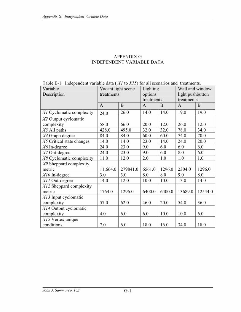
Appendix G: Independent Variable Data
John J. Sammarco, P.E
G-1
APPENDIX G INDEPENDENT VARIABLE DATA
Table E-1. Independent variable data ( X1 to X15) for all scenarios and treatments.
Vacant light scene treatments
Lighting options treatments
Wall and window light pushbutton treatments
Variable Description
A B A B A B X1 Cyclomatic complexity 24.0 26.0 14.0 14.0 19.0 19.0 X2 Output cyclomatic complexity 58.0
66.0
20.0
12.0
26.0
12.0
X3 All paths 428.0 495.0 32.0 32.0 78.0 34.0 X4 Graph degree 84.0 84.0 60.0 60.0 74.0 70.0 X5 Critical state changes 14.0 14.0 23.0 14.0 24.0 20.0 X6 In-degree 24.0 23.0 9.0 6.0 6.0 6.0 X7 Out-degree 24.0 23.0 9.0 6.0 8.0 6.0 X8 Cyclomatic complexity 11.0 12.0 2.0 1.0 1.0 1.0 X9 Sheppard complexity metric 11,664.0
279841.0
6561.0
1296.0
2304.0
1296.0
X10 In-degree 3.0 3.0 8.0 8.0 9.0 8.0 X11 Out-degree 14.0 12.0 10.0 10.0 13.0 14.0 X12 Sheppard complexity metric 1764.0
1296.0
6400.0
6400.0
13689.0
12544.0
X13 Input cyclomatic complexity 57.0
62.0
46.0
20.0
54.0
36.0
X14 Output cyclomatic complexity 4.0
6.0
6.0
10.0
10.0
6.0
X15 Vertex unique conditions 7.0
6.0
18.0
16.0
34.0
18.0

Appendix H: Curriculum Vitae
John J. Sammarco, P.E
H-1
APPENDIX H CURRICULUM VITAE
JOHN J. SAMMARCO, P.E.
54 Standish Boulevard Mt. Lebanon, Pennsylvania 15228
(412) 343-8299; [email protected] Education:
$ Ph.D. ABD, Computer Engineering, West Virginia University, 4.0 GPA $ M.S. Computer Engineering, National Technical University $ M.S. Industrial Engineering, University of Pittsburgh $ B.S. Electrical Engineering Technology, Pennsylvania State University Registration: Professional Engineer, Pennsylvania P.E. No. 32854-E Membership Activities: $ Vice-Chairperson; Institute of Electrical and Electronic Engineers (IEEE)
Committee for Technology Accreditation Activities; Elected position $ Accreditation Evaluator for Computer and Electrical Engineering Technology
Programs; Accreditation Board for Engineering and Technology; Term appointment, 1996-2004
$ Vice-Chairperson; IEEE Industry Applications Society, Mining Industry Committee; Elected position
$ Board Member; MEM Federal Credit Union at Pittsburgh Research Laboratory $ Senior Member, IEEE $ Member, The International System Safety Society
Synopsis of Federal Service: I am an Electrical Engineer at the National Institute for Occupational Safety and Health (NIOSH), Pittsburgh Research Laboratory. My 16 years of Federal service have been devoted to mine safety research in a wide variety of areas including mining machine navigation and guidance, control systems, sensors, system safety, and hazard and risk analysis. The safety of computerized mining systems has been the focus of my research since 1997. Currently, I am Principal Investigator for a project addressing the safety of programmable electronic systems. My international recognitions include a National Science Foundation invitation to lecture in India. At the request of the Australian government, I designed and presented two system safety workshops in Australia and gave the key-note address at the 2000 Australian Mine Electrical Safety Seminar. I was a Session Chair at the 2003 International System Safety Conference in Ottawa, Canada.

Appendix H: Curriculum Vitae
John J. Sammarco, P.E
H-2
JOHN J. SAMMARCO, P.E. Recent Publications: Sammarco, J. J. (2003). Addressing the Safety of Programmable Electronic Mining Systems: Lessons Learned. 2002 IEEE Industry Applications Conference.
Mowrey, G. L., Fries, E. F., Fisher, T. J., & Sammarco, J. J. (2002). Programmable Electronic Mining Systems: Best Practice Recommendations (In Nine Parts); Part 4: 4.0 Safety File. (Report No. IC 9461). Pittsburgh, PA: NIOSH.
Sammarco, J. J. (2002a). A Complexity Assessment Methodology for Programmable Electronic Mining Systems. The 20th International System Safety Conference.
Sammarco, J. J. (2002b). Programmable Electronic Mining Systems: Best Practice Recommendations (In Nine Parts); Part 3: 3.0 Safety File. (Report No. IC 9461). Pittsburgh, PA: NIOSH.
Sammarco, J. J., & Fisher, T. J. (2001). Programmable Electronic Mining Systems: Best Practice Recommendations (In Nine Parts); Part 2: 2.1 System Safety. (Report No. IC 9458). NIOSH.
Sammarco, J. J., Fisher, T. J., Welsh, J. H., & Pazuchanics, M. J. (2000). Programmable Electronic Mining Systems: Best Practice Recommendations (In Nine Parts); Part 1: 1.0 Introduction. (Report No. IC 9456). Pittsburgh, PA: NIOSH.
Sammarco, J. J., Kohler, J. L., Novak, T., & Morley, L. A. (1997). Safety Issues and the Use of Software-Controlled Equipment in the Mining Industry. Proceedings of IEEE Industry Applications Society 32nd Annual Meeting.
Sammarco, J. J. (1999a). Safety Framework for Programmable Electronics in Mining. Mining Magazine. Society of Mining Engineers.
Sammarco, J. J. (1999b). A Systems Safety Approach for Programmable Electronics, Technology News No. 477. NIOSH
Sammarco, J. J. (1997). Progress in Developing Software Safety Guidelines for the Mining Industry. 4th International Symposium on Mine Mechanization and Automation. Brisbane, Australia
32nd Annual IAS/IEEE Meeting "Safety Issues and the Use of Software-Controlled Equipment in the Mining Industry," J. Sammarco, J. Kohler, T. Novak, and L. Morley, New Orleans, LA, (1997).
4th International Symposium on Mine Mechanization and Automation: "Progress in Developing Software Safety Guidelines for the Mining Industry," Brisbane, Australia, (1997).

Appendix H: Curriculum Vitae
John J. Sammarco, P.E
H-3
JOHN J. SAMMARCO, P.E. Recent Awards: Federal Executive Board=s Outstanding Professional Employee - Bronze Award 2003 NIOSH Outstanding Performance Award 2003 NIOSH Outstanding Performance Award 1999 NIOSH Performance Award 1998 NIOSH Performance Award 1997
Federal Executive Board=s Chairman's Award - Silver Award 1997 Federal Executive Board Outstanding Professional Employee - Silver Award 1995