a nonlinear feedback model for tolerance and rebound 1 introduction
TRANSCRIPT

A nonlinear feedback model for
tolerance and rebound
Johan Gabrielsson1 and Lambertus A. Peletier2 3
Abstract
The objectives of the present analysis are to disect a class of turnover feedbackmodels that have proven to be flexible from a mechanistic and empirical point of view,for the characterization of the onset, intensity and duration of response. Specifically,this class of models is designed so that it has the following properties: (I) Stimulationof the production term, which raises the steady state Rss, causes an overshoot anda rebound upon return to baseline. (II) Stimulation of the loss term, which lowersthe steady state Rss, causes an overshoot which is negligible vis-a-vis the reboundupon the return to baseline. (III) Inhibition of the loss term, which raises the steadystate Rss, causes an overshoot which is larger than the rebound upon the return tothe baseline. These models are then anchored in three datasets corresponding tothe cases (I), (II) and (III). The objectives of this paper are to analyze the behaviorof these turnover models from a mathematical/analytical point of view and to makesimulations with different parameter settings and dosing regimens in order to highlightthe intrinsic behavior of these models and draw some general conclusions. We alsoexpand the analysis with two different extensions of the basic feedback model: one witha transduction step in the moderator and one which captures nonlinear phenomena(triggering mechanisms) caused by different drug input rates. A related objectiveis to come up with recommendations about experimental design and model buildingtechniques in situations of feedback systems from a drug discovery point of view.
Keywords: Pharmacokinetic-pharmacodynamic modeling, Feedback, Adaptation, Re-bound, Systems Dynamics, Systems Biology, SSRI, Turnover, Indirect Response.
1 Introduction
In order to characterize the pharmacodynamics of a test compound we want to establishwhat determines the onset, intensity and duration of response, and in the same analy-sis (ideally) separate the systems parameters (turnover rate and fractional turnover rate,feedback capabilities, memory effects, disease) from drug parameters (efficacy and po-tency). The reason why it becomes important to distinguish between systems- and drugcharacteristics is that many test compounds may act on the same system but with dif-ferent potencies or efficiency. In such a case the system parameters stay the same acrosscompounds, but the drug parameters differ. From a systems approach, this has been
1Discovery DMPK, HA232, AstraZeneca R&D Molndahl, S-43183 Molndahl, [email protected] (corresponding author)
2Mathematical Institute, Leiden University, PB 9512, 2300 RA Leiden, The [email protected]
3Centrum voor Wiskunde en Informatica, PB 94079, 1090 GB Amsterdam, The Netherlands
1

thoroughly elaborated for the basic non-tolerant turnover model (Licko and Ekblad [14],Krzyzanski and Jusko [12], [13] and Peletier et. al. [15]). From a drug property point ofview, to make it even more complex, many biological variables, including those affectedby drugs, are subject to adaptive self-regulation. In the description of the time course ofresponse of drugs, it may therefore become necessary to consider the endogenous controlas an integral part of the pharmacodynamics (Ackerman et. al. [1], Urquhart and Li [18],Veng-Pedersen and Modi [16]). Still, the system parameters would ideally be the same fordifferent compounds acting at the same site, but the drug parameters would still differ.Also, in self-regulating systems, the drug input rate may result in very different patternsof adaptation and rebound in spite of the fact that the extent of exposure level is thesame.
In the past there have been several approaches to modeling tolerance and reboundof which some investigators have used time-dependent attenuation of drug parameters(Colburn et. al. [5]), systems analysis (Urquhart and Li [18] and [19], Veng-Pedersenet. al. [16]), pool/precursor (Licko and Ekblad [14], Bauer and Fung [2], Sharma, Eblingand Jusko [17]), and turnover models (Holford et. al. [7], Wakelkamp et. al. [21] andZuideveld et. al. [22]).
In an effort to cast light on phenomena like adaptation (tolerance) and rebound relatedto pharmacological systems, we have chosen to disect a class of turnover feedback modelsthat have proven to be flexible, both from a mechanistic and from an empirical point ofview, for characterization of the onset, intensity and duration of response.
The class of feedback models we focus on here is nonlinear, so that the dynamics ofthese models depends crucially on the state of the system and so changes when it is takenby the drug from the baseline state R0 to a higher or a lower steady state response Rss.Specifically, this class of models is designed so that it has the following properties:
(I) Stimulation of the production term, which raises the steady state Rss, causes an over-shoot and a rebound upon return to baseline.
(II) Stimulation of the loss term, which lowers the steady state Rss, causes an overshootwhich is negligible vis-a-vis the rebound upon the return to baseline.
(III) Inhibition of the loss term, which raises the steady state Rss, causes an overshootwhich is larger than the rebound upon the return to the baseline.
These models are anchored in three datasets corresponding to the cases (I), (II) and(III):
• A dataset displaying a pronounced overshoot of the cortisol secretion rate upon initiationof drug input and a pronounced rebound effect when the exposure to the test compoundis abruptly terminated (Urquhart and Li [18]) (Example I).
• A pharmacodynamic dataset derived from a rapid intravenous infusion of an experi-mental compound with short-acting pharmacokinetics (t1/2 ≈ 1− 3 min) displaying bothtolerance, rebound and return to baseline (Example II).
• A recently applied model for serotonin (5-HT) turnover in rat brains during intravenousadministration of selective serotonin reuptake inhibitors (SSRI’s) (Bundgaard et. al. [4])(Example III).
2

Characteristic response-time plots for these three examples are shown in Figure 1.R
esp
on
se
Time
Baseline
Example III
ktol << kout
Time
Baseline
Example I
ktol ! kout
Time
Baseline
Example II
ktol < kout
Figure 1: Schematic illustration of model behavior in Examples I, II and III. In ExampleI the drug function is piecewise constant. In Examples II and III the drug function is aconstant rate intravenous infusion followed by washout. The plasma kinetics of the testcompound in Example II is very rapid (half life less that 2 min) thereby appearing aspiecewise constant
It is the characteristic shape of these response curves: an overshoot with respect to thenew pharmacodynamic steady state, a steady state which is different from the baseline, arebound upon return to the baseline, and the difference in magnitude of these two, whichwe want to study in this paper.
An important factor in determining the size of overshoot or rebound is found to bethe rate of input or loss of test compound in relation to the intrinsic rates of the system:rapid input or loss tends to cause a large overshoot/rebound, whilst gradual input or losstends to confound overshoot/rebound. Thus, we first focus on stepwise changes of the testcompound in order to extract the intrinsic properties of the pharmacodynamic system(Examples I and II), and then study the effect of more gradual plasma concentrationprofiles of the compound (Example III).
The objectives of this paper are to analyze the behavior of these turnover models froma mathematical/analytical point of view and to make simulations with different parametersettings and dosing regimens in order to highlight the intrinsic behavior of these models anddraw some general conclusions. We also expand the analysis with two different extensionsof the basic feedback model: one with a transduction step in the moderator and one whichcaptures nonlinear phenomena (triggering mechanisms) caused by different drug inputrates.
It will prove illuminating to study the evolution of the system in State Space, whichfor these models is two-dimensional, the dimensions being the response R and the mod-erator M . We shall see that the structure of the state space, also refered to as the phaseplane, immediately reveals the tendency of the system towards overshoot when the systemjumps to a higher value of the steady state of the response.
A related objective is to come up with recommendations about experimental designand model building techniques in situations of feedback systems from a drug discoverypoint of view.
3

The plan of the paper is the following. In Section 2 we briefly describe the threeexamples which anchor the analysis of the class of feedback models, and we present typicalvalues of the model parameters involved. In Sections 3 and 4 we present a qualitativeanalysis of this class of models: in Section 3 for simple piecewise constant exposure profiles,and in Section 4 for more slowly varying exposure profiles. There we show that reducingthe rate of increase of the plasma concentration can confound overshoot and rebound.In Section 5 we show how overshoot can act as a trigger for different types of long timebehavior of nonlinear turnover models. In Section 6 we discuss the identifyablility questionwhether the model parameters featuring in the two models can be determined from theresponse-time plots. In Section 7 we present a generalization of our models involving acascade of two moderators which proved to be effective in the simulations of Examples IIand III. Finally, in Section 8, we summarize and discuss the main results. Many of theresults formulated in Sections 3, 4, 5, 6 and 7 are proved in detail in two Appendices atthe end of the paper.
2 Three Examples
In this section we describe three specific examples which exhibit the type of phenomenawhich we study in this paper.
2.1 Example I: Cortisol Secretion Model
This example is based on data obtained by Urquhart and Lin [19] and [18] from ex vivoexperiments involving adrenocortical secretion in response to a stepwise infusion of adreno-corticotropin (ACTH): the ACTH concentration C was raised from 1 to 2 µU/mL over aperiod of about 60 minutes. The resulting data are shown in Figure 2.
2.pdf
1.5
2.0
2.5
3.0
3.5
4.0
4.5
20 40 60 80 100 120 140 160 180
Time (min)
Figure 2: Observed (filled symbols) and model predicted (solid line) cortisol secretion rateversus time. Data scanned from Urquhart and Lin [19] and model from the system (I)(Gabrielsson and Weiner 2006 [6]) with parameter values from Table 1
In [19] this system was modeled by means of a linear feedback system involving theCortisol secretion rate, R, and a feedback moderator M . In this paper we propose a
4

nonlinear feedback system in which the response R acts linearly on the production (ktol)of the moderator (M), which acts inversely on the production (kin) of response. Theplasma kinetics serves as input to a stimulating function acting on the production ofresponse. This leads to the following system of differential equations for R and M
(I)
dR
dt=
kin
MS(C)− koutR
dM
dt= ktol(R−M)
where S(C) = Cn (2.1)
in which kout and ktol are first-order rate constants. Here C is either 1 or 2.Fitting the parameter values to the data set yields the values given in Table 1 in which
the rate constants kout, ktol are measured in min−1. In Table 1, R0 denotes the baselineof the response, kin = R2
0kout (cf. Section 3), and κ = ktol/kout. A simulation for thesevalues is also shown in Figure 2.
Table 1: Parameter estimates of System (I)
R0 kout ktol n κ2.05 0.16 0.18 0.78 1.1252 % 5 % 14 % 6 % –
Typical characteristics of the response-time curve are (i) a steep rise and significantovershoot at the onset of the infusion, (ii) a period over which the response remainsrelatively constant, and (iii) a sharp drop below the baseline and a rebound at terminationof the infusion.
2.2 Example II: Compound X
The second example is based on an experimental compound with fast plasma kinetics(t1/2 ≈ 4 minutes, kel = 0.17 min−1) and a pharmacological response R with high kout
(t1/2 ≈ 3 minute) that also displays tolerance and rebound. The resulting data are shownin Figure 3.
0.0
0.5
1.0
1.5
2.0
0 20 40 60 80 100 120 140 160
Time (min)
Figure 3: Observed (filled symbols) and model predicted (solid line) response versus time.Data from compound X and model from system (II) with parameter values from Table 2
Modeling this process leads to a feedback system similar to the one used in ExampleI, but one in which the compound stimulates the loss term. Specifically, it leads to the
5

following system of differential equations:
(II)
dR
dt=
kin
M− koutR · S(C)
dM
dt= ktol(R−M)
where S(C) = 1 + Cn/A (2.2)
in which A and n are drug parameters. Estimates for numerical values of the differentdrug and model parameters obtained in experiments are listed in Table 2.
Table 2: Parameter estimates of System (II)
R0 kout ktol kel A n κ1.1 0.17 0.04 0.17 3.8 0.0015 0.2355 % 135 % 127 % – 171 % 31 % —
In Figure 3 we observe a negligible overshoot at the onset of drug exposure but a morepronounced rebound upon cessation of drug exposure.
2.3 Example III: A model for Selective Serotonin Reuptake Inhibition
Our third example stems from a recently developed feedback turnover model for SelectiveSerotonin Reuptake Inhibition (SSRI) (Bundgaard et. al. [4], see also Holford et al. [7]).The model mimics drug induced effects on brain extracellular levels of serotonin (5-HT)after constant rate infusions of the SSRI Escitalopram (S-Citalopram) in rats.
In Figure 4 we show the model fits (3 lower curves) superimposed on experimentaldata (observations: symbols). In addition, we show a model simulation (upper curve) fora system lacking tolerance.
0
100
200
300
400
500
600
0 50 100 150 200 250 300 350 400
Time (min)
Figure 4: Observed (filled symbols) and model predicted (solid line) response (change of5-HT from baseline) after three different constant intravenous infusions of escitalopram torats followed by washout. Data from Bundgaard et. al. [4] and model from the system(III) with parameter values listed in Table 3. The predicted single top line denotes asimulation of a model which does not display tolerance, using the highest dose
6

The dynamics of escitalopram-evoked changes of 5-HT response was characterized bya turnover model, which included an inhibitory feedback moderator component:
(III)
dR
dt=
kin
M− koutR · I(C)
dM
dt= ktol(R−M),
(2.3)
in which kout and ktol are first-order rate constant. Here, the drug mechanism function isgiven by
I(C) = 1− ImaxCn
ICn50 + Cn
(2.4)
where 0 < Imax ≤ 1, and IC50 and n are positive constants. Estimates for the modelparameters are given in Table 3.
Table 3: Parameter estimates of System (III)
R0 kout ktol Imax IC50 n κ112 0.16 0.0010 0.86 4.6 0.99 0.00695 % 13 % 46 % 2 % 26 % 12 % —
Typical characteristics of the data set are (i) a rapid upswing without overshoot, (ii)almost superimposable response-time curves for the higher doses due to tolerance, and(iii) no rebound during the terminal response-time course due to the extended declinein the exposure to escitalopram. In other words, the comparatively slow change in theexposure pattern to escitalopram confounds the system behavior (overshoot/rebound) of5-HT turnover. Still, fitting the three response-time courses enables one to mimic theexperimental data and to obtain robust and precise parameter estimations.
3 Qualitative analysis
Examples II and III are special cases of the class of feedback systems:
(FB)
dR
dt=
kin
M− koutR ·H(C)
dM
dt= ktol(R−M)
(3.1)
where kin, kout and ktol are positive rate constants. In Example III the drug mechanismfunction H(C) is inhibitory and given by I(C) (cf. (2.4)) and in Example II it stimulatingand given by S(C) (cf. (2.2)). Throughout we assume that I(C) is a decreasing functionand that S(C) is increasing.
In this section we establish characteristic properties of the response-time curves, thelevel Rmax and time Tmax of the maximal response, and the effect of the different param-eters in the system and the drug mechanism functions. Many of the results formulated inthis section are proved in Appendix B.
We begin with a few preliminary observations about the system (3.1), and then turnto a more detailed account of the two cases: H(C) = I(C) and H(C) = S(C).
7

3.1 Preliminaries
We shall find that the intrinsic properties of (3.1) are significantly affected by the drugfunction. Thus, in order to focus on these intrinsic properties we first consider plasmaconcentrations C(t) which correspond to stepwise dosing regimens. Specifically, we con-sider:
(a) A constant infusion: C(t) ≡ Css for t ≥ 0, where Css ≥ 0.
(b) Onset of an infusion at time t1 ≥ 0:
C(t) = CssH(t− t1) where 0 ≤ t1 <∞ (3.2)
(c) Onset of an infusion at time t1, and subsequent termination (washout) at t = t2:
C(t) = Css{H(t− t1)−H(t− t2)} where 0 ≤ t1 < t2 <∞ (3.3)
Here H(s) denotes the Heaviside function: H(s) = 0 if s < 0 and H(s) = 1 if s ≥ 0. In thenext section we expand our analysis to more general drug functions, especially functionswhich vary more gradually.
Note that the system (3.1) is nonlinear in that the zeroth order growth term of the firstequation depends nonlinearly on the moderator M . This means that the usual meaning ofthe constant kin as a zeroth order rate constant with dimension [R]/[t] no longer applies.Still, it will prove convenient to stick with the constant kin although its interpretation isdifferent from the classical one.
Thus, let us first assume that the plasma concentration C is fixed. Then there existsa unique pharmacodynamic steady state, which is given by
Rss = Mss =
√kin
koutH(C)(3.4)
If H(C) = I(C), then – because I(C) decreases with C – the steady state values Rss
and Mss are increasing functions of the plasma concentration C. If H(C) = S(C), then– because S(C) increases with C – the steady state values Rss and Mss are decreasingfunctions of C.
We obtain the baseline value (R0,M0) of the steady state by putting C = 0. Thisyields
R0 = M0 =√
kin
kout(3.5)
Thus, the relative values of Rss and Mss with respect to their baseline values are given by
Rss
R0=
Mss
M0=
1√H(C)
(3.6)
When C is frozen the equilibrium state (Rss,Mss) is stable. In fact, it is a globalattractor in that, given any initial state, the solution will eventually converge towards(Rss,Mss).
8

Theorem 3.1 Let (R(t),M(t)) be the solution of the system (3.1) with ktol > 0, whichevolves from an arbitrary initial state. Then
R(t)→ Rss and M(t)→Mss as t→∞ (3.7)
For the proof we refer to Appendix B (Theorem B.2).
Examples I & III Example II
0 100 200 300 400 500 600 700 800 900 10000
100
200
300
400
500
600
Time
Response/Moderator
0 5 10 15 20 25 300
20
40
60
80
100
120
Time
Response/Moderator
Figure 5: Typical graphs of the response R(t) (solid line) and the moderator M(t) (dashedline) after an abrupt raise in drug level, shown for inhibition and stimulation of the lossterm (kin = 1600, kout = 0.16, ktol = 0.0016 (left), ktol = 0.12 (right) and Imax = 0.95,Smax = 4)
In Figure 5 we show how R(t) and M(t), starting from the baseline (R0,M0), evolve withtime and converge towards the steady state (Rss,Mss). We see that here the curves for Rexhibit overshoot, while the curves for M are monotone.
An alternative way to analyze the dynamical behavior of system (3.1) is to follow thestate of the system, which is determined by the pair (R, M), as it traces out an orbit instate space, i.e., in the (R,M)-plane. In Figure 6 we show the orbits in the phase planewhich correspond to the response-time and moderator-time graphs shown in Figure 5.Starting from the baseline (R0,M0) we see that in both cases the orbit loops towards thesteady state (Rss,Mss) as t→∞, as predicted by Theorem 3.1.
In addition to the orbits, we have drawn the Null Clines, the curves along whichdR/dt = 0 – denoted by ΓR – and the curves along which dM/dt = 0 – denoted by ΓM .Thus, as we see demonstrated in Figure 6, the orbit intersects ΓR horizontally and ΓM
vertically. For the system (3.1) the null clines are given by
ΓR :kin
M− koutR ·H(C) = 0 a hyperbola
ΓM : R−M = 0 a straight line(3.8)
We see that ΓR depends on the value of C: if H(C) = I(C) it shifts up when C increases,and if H(C) = S(C) it shifts down when C increases.
Plainly, ΓR and ΓM have precisely one point of intersection in the first quadrant. Thispoint corresponds to the unique equilibrium point (Rss,Mss) defined in (3.4).
9

Examples I & III Example II
XX0 50 100 150 200 250 300 3500
100
200
300
400
500
600
Moderator
Response
0 20 40 60 80 100 1200
20
40
60
80
100
120
Moderator
Response
Figure 6: Evolution of the state (Response R(t) versus Moderator M(t)) time courses ofthe system represented as an orbit in the (R,M)-plane (solid line), shown for inhibitionand stimulation of the loss term when ktol > 0. The dashed lines are the null clines ΓR
and ΓM ; parameter values as in Figure 5
We conclude these preliminaries with the introduction of a dimensionless constant κwhich is defined as the ratio of the different time scales involved in the equations for Rand M ,
κ =ktol
kout
We shall see that this ratio is critical for the qualitative properties of the dynamics of(3.1).
We now turn to a more detailed study of (3.1) for the cases in which the loss term isinhibited or stimulated. For the sake of transparency we discuss these cases separately.
3.2 Inhibition of the loss term
In Figure 7 we give a schematic picture of the response curve following a step functionwhich basically mimics an infusion and subsequent washout for a compound with veryrapid kinetics. By applying a step function (rapid changes in the increase and washout ki-netics) it is possible to display the pharmacodynamic system properties, such as overshootat the onset and rebound at washout. The different characteristic values of the response,such as the pharmacodynamic steady state Rss are indicated in the picture.
We first focus on the onset of a drug input, i.e., we assume that C(t) is of type (b) witht1 = 0, and that the response R and the moderator M start from the baseline: R(0) = R0
and M(0) = M0.In order to study the effect of the moderator M on the time course of the response,
it is instructive to first discuss the extreme case: ktol = 0. Then dM/dτ = 0 and themoderator stays at its baseline value, i.e., M(t) = M0 for all t > 0. This means that inthe phase plane the orbit is parallel to the R-axis, i.e., vertical (see Figure 9).
For M(t) ≡M0 the equation for R becomes
dR
dt=
kin
M0− koutR · I(Cmax) (3.9)
10

ΔR
Rss
R0
Overshoot
Response
Time
Rebound
Rmax
Rtop
Rbottom
Figure 7: Schematic picture of the response versus time curve due to a stepwise plasmaconcentration profile (Gray bar along the time axis), i.e., when C(t) is of type (c)
Thus, the model is reduced to the classical indirect response model in which kin is replacedby kin/M0. The equilibrium solution of this equation, which we denote by Rtop is givenby the zero of the right hand side of (3.9), i.e.,
Rtop =1
I(Css)kin
kout
1M0
=R0
I(Css)(3.10)
Note that the point (Rtop,M0) is the intersection of the vertical line through the baselinepoint (R0,M0) and the null cline ΓR (see Figure 9).
Let us denote the solution of (3.9), which starts at R0, by R(t). We readily see thatthis solution converges to Rtop as t→∞:
R(t)↗ Rtop as t→∞ (3.11)
Since R(t) is increasing, there is no tolerance in this case.
We now take ktol > 0, so that M(t) is no longer constant and the orbit in the phaseplane is no longer vertical. We may now apply Theorem 3.1 to conclude that
R(t)→ Rss as t→∞
however small ktol may be.The orbit in the phase plane (cf. Figure 9) shows that M(t) > M0 for all t > 0. This
lower bound for M(t) enables us to use a comparison argument (cf. [15]) to establish thefollowing upper bound for R(t):
Theorem 3.2 Let (R(t),M(t)) be the solution of (3.1) which starts at the baseline (R0,M0).Suppose that ktol > 0. Then
R(t) < R(t) for all t > 0 (3.12)
Theorem 3.2 will be proved in Appendix B (Theorem B.3).
11
0 50 100 150 200 250 300 350 400 450 5000
100
200
300
400
500
600
700
800
900
Time
Response/Moderator
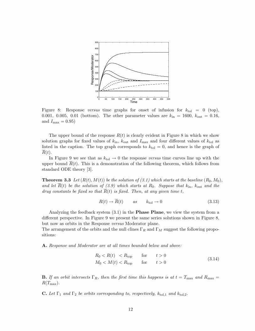
Figure 8: Response versus time graphs for onset of infusion for ktol = 0 (top),0.001, 0.005, 0.01 (bottom). The other parameter values are kin = 1600, kout = 0.16,and Imax = 0.95)
The upper bound of the response R(t) is clearly evident in Figure 8 in which we showsolution graphs for fixed values of kin, kout and Imax and four different values of ktol aslisted in the caption. The top graph corresponds to ktol = 0, and hence is the graph ofR(t).
In Figure 9 we see that as ktol → 0 the response versus time curves line up with theupper bound R(t). This is a demonstration of the following theorem, which follows fromstandard ODE theory [3].
Theorem 3.3 Let (R(t),M(t)) be the solution of (3.1) which starts at the baseline (R0,M0),and let R(t) be the solution of (3.9) which starts at R0. Suppose that kin, kout and thedrug constants be fixed so that R(t) is fixed. Then, at any given time t,
R(t)→ R(t) as ktol → 0 (3.13)
Analyzing the feedback system (3.1) in the Phase Plane, we view the system from adifferent perspective. In Figure 9 we present the same series solutions shown in Figure 8,but now as orbits in the Response versus Moderator plane.The arrangement of the orbits and the null clines ΓR and ΓM suggest the following propo-sitions:
A. Response and Moderator are at all times bounded below and above:
R0 < R(t) < Rtop for t > 0M0 < M(t) < Rtop for t > 0
(3.14)
B. If an orbit intersects ΓR, then the first time this happens is at t = Tmax and Rmax =R(Tmax).
C. Let Γ1 and Γ2 be orbits corresponding to, respectively, ktol,1 and ktol,2.
12

0 50 100 150 200 250 300 3500
100
200
300
400
500
600
700
800
900
Response
Moderator
Figure 9: Orbits in the (R,M)-plane for onset of infusion for ktol = 0(vertical), 0.001, 0.005, 0.01; the other parameter values are as in Figure 8. Note howthey all start at the baseline (R0,M0) = (100, 100) and, except when ktol = 0, end up atthe steady state (Rss,Mss)
(a) Γ1 and Γ2 cannot intersect before they leave the region enclosed by ΓM , ΓR and Γ0 ={(R,M) : M = M0} (see Figure 9).
(b) Suppose that0 < ktol,1 < ktol,2
Then, until Γ1 intersects ΓR, Γ1 lies in the region enclosed by Γ0, ΓR and Γ2.
D. Let Rmax,1 and Rmax,2 be the maximal response on, respectively, Γ1 and Γ2. Then
ktol,1 < ktol,2 =⇒ Rmax,1 > Rmax,2 (3.15)
These propositions are indeed correct and will all be proved in Appendix B.
Remark. Propositions C and D hold under the assumption that kin and kout as wellas the drug constants are the same for Γ1 and Γ2. A more general result, in which therestriction on kin and kout is dropped, is:
κ1 < κ2 =⇒ Rmax,1
R0,1>
Rmax,2
R0,2(3.16)
where R0,1 and R0,2 are the baseline values of Γ1 and Γ2 (cf. Theorem B.4).
Tolerance. It is evident from the phase plane that if an orbit intersects ΓR, then Rmax >Rss, so that there is tolerance. It follows from Theorem 3.3 that for small values of ktol
the orbit intersects ΓR. Moreover,
Rmax → Rtop as ktol → 0
Hence, tolerance can approach, but not exceed, the value
∆R∣∣∣overshoot
= Rtop −Rss = R0
(1
I(Css)− 1√
I(Css)
)(3.17)
13

A good measure of the ”size” of the overshoot is the ratio of the upper bound Rtop
above the baseline R0, and the steady state value Rss above the baseline. From (3.6) and(3.10) we conclude that this ratio is given by
Rtop −R0
Rss −R0= 1 +
1√I(Css)
(3.18)
We still have not answered the question as to whether there is tolerance for all ktol > 0.The anser is negative and we shall prove the following criterium for tolerance.
Theorem 3.4 The response-time graph has a maximum, i.e., there is tolerance, if ktol <k+
tol = (3 + 2√
2)I(Css)kout. There exists a constant k∗tol ≥ k+tol such that if ktol > k∗tol then
the graph is monotone, and there is no tolerance.
Theorem 3.4 is proved at the end of Appendix B.
Next we consider the case of washout, i.e., C(t) is of type (c). We now assume thatprior to washout, the system is at the steady state, i.e., R = Rss and M = Mss. Focussingon the extreme case again, we assume that ktol = 0 so that M(t) = Mss for all t > 0. Asbefore we obtain a turnover equation such as (3.9) and we find that R(t) → Rbottom (cf.Figure 7) as t→∞, where
Rbottom =kin
kout
1Mss
= R0
√I(Css) (3.19)
Arguing as before we see that at washout tolerance can never exceed
∆R∣∣∣rebound
= R0 −Rbottom = R0{1−√
I(Css)} (3.20)
We conclude from (3.17) and (3.20) that the following important relation holds betweenthe two extreme values for tolerance at input and at washout:
Theorem 3.5 We have
∆R∣∣∣overshoot
=1
I(Css)∆R
∣∣∣rebound
(3.21)
Thus, since in the experiments in Bundgaard [4] (Example III) the value Imax = 0.86 hasbeen used, the maximal overshoot may exceed the maximal rebound by up to a factor 7.
Asymptotics. We complete this subsection with an heuristic asymptotic analysis of theresponse versus time curves in the two extreme cases, κtol + κout and κtol , κout, andassume for convenience that kout is kept fixed, while κtol is chosen either small or large.
Case (i): ktol + kout. As we have seen, in this case the orbit consists of a rapid risetowards ΓR, in which, by Theorem 3.3 R(t) ≈ R(t), followed by a much slower descentalong ΓR towards the steady state (Rss,Mss). Thus R(t) reaches a maximum value Rmax
14

at some finite time Tmax. Since R(t)→ R(t) for fixed t, and R(t) is increasing, it is clearthat Rmax tends to Rtop as ktol → 0.
During the slow descent, dR/dt ≈ 0 and so R(t) and M(t) approximately satisfy therelation
kin
M− koutR · I(Css) = 0 (3.22)
When we use this to eliminate R from the equation for M , we obtain the nonlinear equation
dM
dt= ktol
(R2
0
I(Cmax)1M−M
)(3.23)
This equation can be solved explicitly and, assuming that M(Tmax) ≈M0, we find that
M(t) =M0√I(Css)
{1− [1− I(Css)]e−2ktol(t−Tmax)
}1/2, t > Tmax (3.24)
and hence, by (3.22),
R(t) = Rss
{1− [1− I(Css)]e−2ktol(t−Tmax)
}−1/2t > Tmax (3.25)
This expression shows that the solution (R(t),M(t)) moves towards the steady state(Rss,Mss) with a rate constant 2ktol.
Thus, summarizing, first R(t) increases to approximately Rtop with a rate constantkout whilst M(t) ≈ M0. Then R(t) and M(t) move in tandem towards their respectivefinal steady states Rss and Mss with the much smaller rate constant 2ktol.
Case (ii): ktol , kout. The rate constant of the equation for R is now much smallerthan the one of the equation for M . This means that the orbit follows ΓM , so that,approximately,
R(t)−M(t) = 0 for all t ≥ 0 (3.26)
We use this equality to eliminate M from the equation for R. This yields the nonlinearturnover equation:
dR
dt=
kin
R− koutR · I(Css) (3.27)
which has the same form as (3.23) and yields the solution
R(t) = Rss
{1− [1− I(Css)]e−2koutI(Css)t
}1/2(3.28)
It is readily seen that R(t) is strictly increasing for all t ≥ 0. Therefore, in this limitingcase there is no overshoot, as predicted by Theorem 3.4.
15
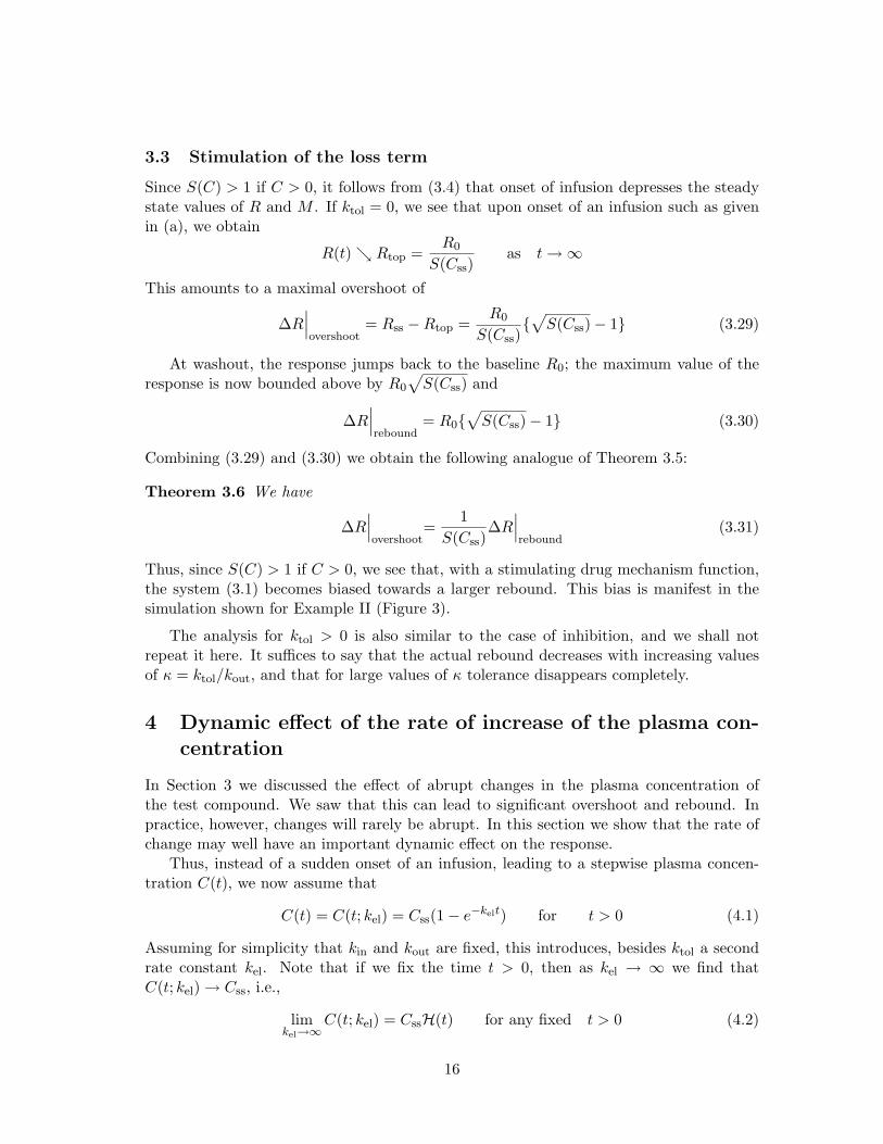
3.3 Stimulation of the loss term
Since S(C) > 1 if C > 0, it follows from (3.4) that onset of infusion depresses the steadystate values of R and M . If ktol = 0, we see that upon onset of an infusion such as givenin (a), we obtain
R(t)↘ Rtop =R0
S(Css)as t→∞
This amounts to a maximal overshoot of
∆R∣∣∣overshoot
= Rss −Rtop =R0
S(Css){√
S(Css)− 1} (3.29)
At washout, the response jumps back to the baseline R0; the maximum value of theresponse is now bounded above by R0
√S(Css) and
∆R∣∣∣rebound
= R0{√
S(Css)− 1} (3.30)
Combining (3.29) and (3.30) we obtain the following analogue of Theorem 3.5:
Theorem 3.6 We have
∆R∣∣∣overshoot
=1
S(Css)∆R
∣∣∣rebound
(3.31)
Thus, since S(C) > 1 if C > 0, we see that, with a stimulating drug mechanism function,the system (3.1) becomes biased towards a larger rebound. This bias is manifest in thesimulation shown for Example II (Figure 3).
The analysis for ktol > 0 is also similar to the case of inhibition, and we shall notrepeat it here. It suffices to say that the actual rebound decreases with increasing valuesof κ = ktol/kout, and that for large values of κ tolerance disappears completely.
4 Dynamic effect of the rate of increase of the plasma con-centration
In Section 3 we discussed the effect of abrupt changes in the plasma concentration ofthe test compound. We saw that this can lead to significant overshoot and rebound. Inpractice, however, changes will rarely be abrupt. In this section we show that the rate ofchange may well have an important dynamic effect on the response.
Thus, instead of a sudden onset of an infusion, leading to a stepwise plasma concen-tration C(t), we now assume that
C(t) = C(t; kel) = Css(1− e−kelt) for t > 0 (4.1)
Assuming for simplicity that kin and kout are fixed, this introduces, besides ktol a secondrate constant kel. Note that if we fix the time t > 0, then as kel → ∞ we find thatC(t; kel)→ Css, i.e.,
limkel→∞
C(t; kel) = CssH(t) for any fixed t > 0 (4.2)
16

Thus, for large values of kel we expect to retrieve the results of Section 3.In this section we focus on the system (3.1) in which we assume that
H(C) = I(C) = 1− ImaxC(t) where ImaxCss < 1 (4.3)
In Figure 10 we show simulations of this model and we see how the overshoot which existsfor kel = 0.05 rapidly disappears when the elimination rate drops down to kel = 0.002.
0 100 200 300 400 500 600 700 800 900 1000100
150
200
250
300
350
400
450
500
550
Time
Response/Moderator
Figure 10: Response versus time graphs of system (3.1) (H = I) with I(C) given by (4.3),kel = 0.05, 0.01, , 0.005, 0.002 and kin = 1600, kout = 0.16, ktol = 0.0016, Imax = 0.95
Here we shall only discuss one, extreme, case, the one in which we assume that thethree rate constants are ordered according to
(a) ktol + kout and (b) kel + ktol (4.4)
As in Section 3, we conclude from (a) that, after a very short time of O(k−1out), the orbit
reaches the null-cline ΓR after which R(t) and M(t) are approximately related by
kin
M− koutR · I(C(t)) = 0 (4.5)
When we use this relation in order to eliminate R from the equation for M , we obtain
dM
dt= ktol
(R2
0
I(C(t))1M−M
)(4.6)
This equation is similar to (3.23) and can, in principle, be solved explictly. However, evenwithout an explicit solution, we see by inspection that M(t) increases monotonically toMss.
Plainly, the function I(C(t)) in the right hand side of (4.6) changes at a time scale ofO(k−1
el ). This is slow in comparison with the time scale O(k−1tol ) on which M(t) will vary
initially. Thus after a brief time of O(k−1tol ), the right hand side of (4.6) vanishes and we
have approximatelyR2
0
I(C(t))1
M(t)−M(t) = R(t)−M(t) = 0
17

Since we have seen that M(t) is increasing, we conclude that R(t) is increasing too. Thus,the conditions (4.4) on the rate constants imply that in the limit when
ktol/kout → 0 and kel/ktol → 0
there will be no overshoot.In this section we have only scratched the surface. It will be interesting to carry out a
more comprehensive study of the effect of the two critical constants κ and kel/kout on thecharacter of the response-time curve and to find out in which ranges their impact is mostsignificant.
5 A trigger mechanism
Clinical evidence suggests that the physiological effect of certain drugs may depend on thedosing regimen employed ([9], [10], [11], [20]). In [11] this observation has been studied bymeasuring the hemodynamic effect of nifedipine for two different dosing regimens:
(i) in the form of rapidly dissolving capsules, resulting in a rapid increase in the plasmaconcentration-time profile, and
(ii) in the form of sustained release tablets, giving a more slowly increasing, concentrationprofile.This resulted in a rapid and a slow rise of the plasma concentration, respectively. Thedoses were so chosen that eventually, both regimens resulted in comparable plasma con-centrations. The differences in the effect were pronounced: the rapid increase led to arapid rise in heart rate (HR) and a slight drop in blood pressure (BP), whilst the slowincrease did not lead do a significant rise in HR but did lead to a sustained and substantialdrop in BP.
These experiments suggests that, given a steady plasma concentration of the com-pound, the system can exist in one of two stable physiological steady states. At the onsetof the infusion, depending on the manner the plasma concentration reaches its constantvalue, the system would end up in one or the other steady state.
In this section we propose a conceptual mechanism that could - in principle - explainhow the gradient of the plasma concentration profile can trigger one type of behavior oranother. The hypothetical mechanism we put forward can be divided into three parts:
(I) A given concentration profile of the compound C(t);
(II) A feedback system such as (3.1) driven by the compound, which results in a responsewhich we denote by P (t), and
(III) A turnover model driven by the function S(P (t)), where S(P ) is an increasing functionof P , in which the loss term involves a nonlinear function f(R). This leads to the equation
dR
dt= kinS(P (t))− koutf(R) (5.1)
We assume that C = 0 implies that P = P0, the baseline for the feedback model, andthat S(P0) = 1. Finally, we assume that the baseline R0 for equation (5.1) is given by
18
R0 = kin/kout. This is the case when R0 is a solution of the equation
kin − koutf(R) = 0
i.e., if
f(R0) =kin
kout= R0
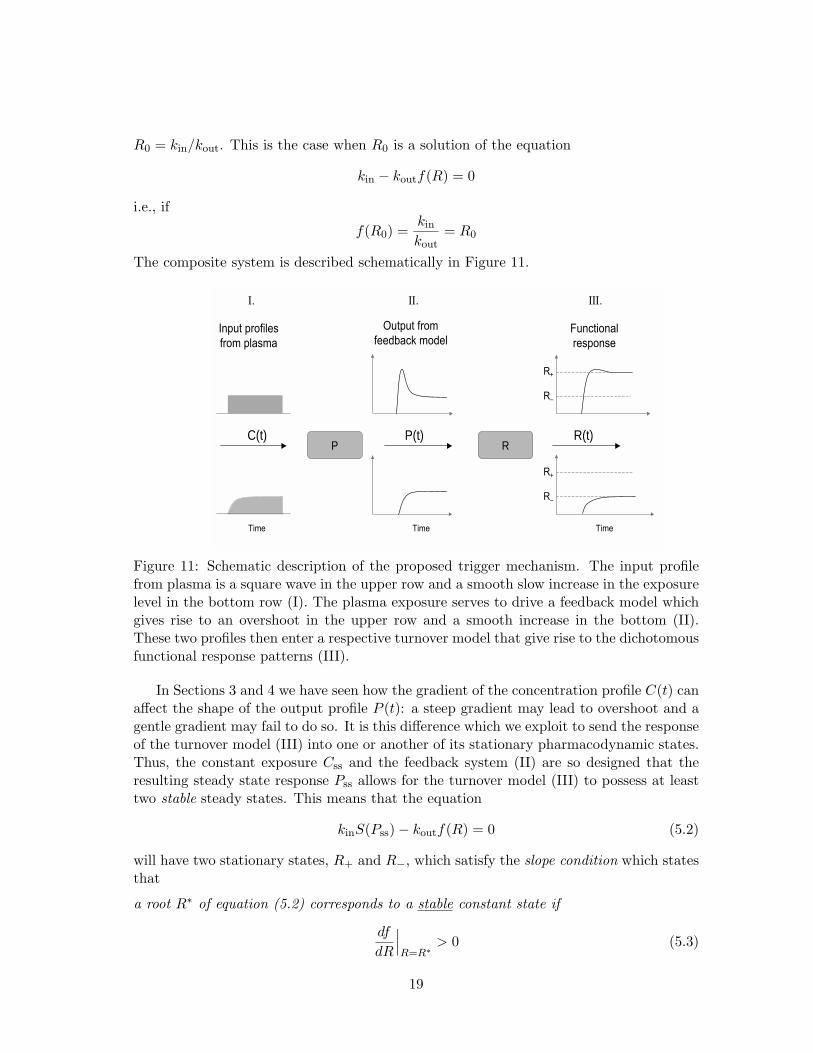
The composite system is described schematically in Figure 11.
P R
Input profiles
from plasma
Output from
feedback modelFunctional
response
I. II. III.
R+
TimeTimeTime
C(t) P(t) R(t)
R–
R+
R–
Figure 11: Schematic description of the proposed trigger mechanism. The input profilefrom plasma is a square wave in the upper row and a smooth slow increase in the exposurelevel in the bottom row (I). The plasma exposure serves to drive a feedback model whichgives rise to an overshoot in the upper row and a smooth increase in the bottom (II).These two profiles then enter a respective turnover model that give rise to the dichotomousfunctional response patterns (III).
In Sections 3 and 4 we have seen how the gradient of the concentration profile C(t) canaffect the shape of the output profile P (t): a steep gradient may lead to overshoot and agentle gradient may fail to do so. It is this difference which we exploit to send the responseof the turnover model (III) into one or another of its stationary pharmacodynamic states.Thus, the constant exposure Css and the feedback system (II) are so designed that theresulting steady state response Pss allows for the turnover model (III) to possess at leasttwo stable steady states. This means that the equation
kinS(Pss)− koutf(R) = 0 (5.2)
will have two stationary states, R+ and R−, which satisfy the slope condition which statesthat
a root R∗ of equation (5.2) corresponds to a stable constant state if
df
dR
∣∣∣R=R∗
> 0 (5.3)
19

to ensure that R+ and R− are stableIn Figure 12 we show two examples of functions f(R): on the left, the linear increasing
function f(R) which features in the classical turnover model, and on the right a nonlinearnon-monotone function f(R). It is clear from Figure 12 that if f(R) is given by the linearfunction, then equation (5.2) has precisely on zero, Rss which satisfies the slope condition(5.3). On the other hand, if f(R) is given by the nonlinear function (on the right) it hasthree roots, two of which – denoted by R+ and R− – satisfy the slope condition (5.3). As
f(R)
R
f(R)
R
R– R+
R0S(Pss) R0S(Pss)
Rss
Figure 12: Two functions f(R): A linear function (left) and a nonlinear non-monotonefunction for which (5.2) has two zeros R+ and R− which satisfy (5.3)
an example of a function as depicted in Figure 12 we propose the function
f(R) = kR
R250 + R2
+ koutR (5.4)
in which k, R50 and kout are suitably chosen paramters (e.g. k = 1, R50 = 0.01 andkout = 3).
Next we turn to the dynamics of the nonlinear turnover model (5.1). In order todemonstrate how the size of the overshoot of the trigger function P (t) can affect the largetime behavior of the response R(t), we do simulations on an artificial example, selectednot so much for its mechanistic relevance, but rather for its ability to demonstrate themathematical phenomenon we wish to point out effectively.
Thus, for f(R) we choose the function
f(R) =(R− r)3 − (R− r)
1 + (R− r)2+
r3 − r
1 + r2, where r =
32
(5.5)
Note that f(0) = 0 and that generally, the graph of f(R) looks very much like the one inthe figure on the right in Figure 12. When we put kin = 0.15 and kout = 0.26 we find thatequation (5.1) has two constant stable states: R+ = 2.5 and R− = 0.5.
For the functions S(P ) and P (t) we take
S(P ) = 1 + (P − P0) and P (t) = P0 + A(e−k1t − e−k2t) (5.6)
In the simulations shown in Figure 13 we exhibit response versus time curves of theturnover equation (5.1) subject to the initial condition, R(0) = R− = 0.5 for differentstrengths of the function P (t), i.e. for values of the coefficient A in (5.6). We see howdifferent P versus time profiles can send the response of the turnover model (5.1) eithertowards R+ or towards R−.
We conclude that in principle a concatenation of a feedback systems such as (3.1) anda nonlinear turnover model such as(5.1) can translate different concetration gradients intodifferent final pharmacodynamic states.
20

P − P0 R
t t
0
0.5
1
1.5
2
2.5
3
0 1 2 3 4 5 60
0.5
1
1.5
2
2.5
3
0 5 10 15 20
(a) P (t)− P0 versus time profiles (b) Response versus time profiles
Figure 13: Plot (a) shows the P (t) − P0 versus time profiles driving the response com-partment; plot (b) shows response versus time profiles as a result of the time courses in(a)
6 Parameter Identifiability
An important issue in experimental design and model building is the identifyability ques-tion as to whether the model parameters can be identified from the available experimentaldata. Focus here is on a system (model) that is able to mimic a single source (R) observa-tional variable, in contrast to a multiple source (R and M or more) system. The latter isexemplified by glucose (R) and insulin (M), which can both easily be measured. Thus, weassume that the data are restricted to response versus time profiles after different dosesof test compound. In this section we shall address this issue for the two models discussedin the previous sections.
For Example III, the parameters we wish to determine are the system parameters, kin
and kout and the drug parameters Imax and IC50. From the response data we readilyobtain estimates for the baseline response R0 (cf. Figure 14).
Also, when C(t) → Css as t → ∞, we easily obtain an estimate for the steady stateRss. From (4.2) and (4.3) we then conclude that in the limit as t→∞,
I(Css) =R2
0
R2ss
=(
R0
Rss
)2
(6.1)
When we do this for two infusions, with concentrations Css,1 and Css,2, we obtain twoequations for the unknown constants Imax and IC50, from which they can be determined.
In order to obtain values for the three rate constants, we note that by (4.2) the baseline value yields one relation between kin and kout:
kin
kout= R2
0 (6.2)
To obtain a second relation, we note that immediately after the onset of the infusion,
dR
dt
∣∣∣t=0+
=kin
M0− koutR0I(Css) =
√kinkout{1− I(Css)} (6.3)
21

Response
Time
{ })C(IkktR
ssoutin −⋅⋅=Δ
Δ 1out
in
kkR =0
topR
ssR
RΔ
−⋅⋅−=
ΔΔ
)C(I)C(Ikk
tR
ssssoutin
1
Figure 14: Schematic illustration of the graphical estimation of initial estimates. The grayhorizontal bar at the bottom denotes the length of drug exposure; R0, Rss and ∆R denotebaseline, steady state response and the difference (clearance) between no regulation Rtop
and regulation Rss, respectively. Slopes at onset and washout are expressed in terms ofthe different parameters
Since dRdt
∣∣∣t=0+
can be estimated and I(Css) is known from (6.1), we thus obtain a secondrelation between kin and kout. From the two relations we deduce the expressions
kin =R0
1− I(Css)dR
dt
∣∣∣t=0+
and kout =1
{1− I(Css)}R0
dR
dt
∣∣∣t=0+
(6.4)
which can be used to estimate kin and kout from the response data.
It remains to estimate ktol. As we have seen in Section 3, an important indication of thesize of ktol, as compared to kout, is the magnitude of the overshoot. When the data showlittle overshoot, then ktol will be comparable or bigger than kout, provided rapid plasmakinetics. On the other hand a large overshoot suggest that ktol + kout. In this case wecan use the approximate expression (3.25) for R(t) to estimate ktol when H(C) = I(C) ora similar expression when H(C) = S(C) . From these expressions we deduce that
R(t) ≈ Rss + Ce−2ktolt as t→∞ (6.5)
where C is some positive constant. Therefore
log{R(t)−Rss} ≈ log(C)− 2ktolt as t→∞ (6.6)
It follows that if ktol + kout, then for larger values of time, as compared to the half lifek−1
out, the slope of the graph of log{R(t) − Rss} versus time yields an initial estimate forktol.
22

Remark In Example III, in which ktol + kout, we find that when we use (6.6) to estimatektol from the log response versus time data, we obtain an initial value for ktol of 0.002minute−1. When we put this value into the WinNonlin regression analysis we obtain thefinal estimate of 0.0011 minute−1 (cf. Table 3a), which is very close.
7 A generalization involving transduction
We propose a refinement of the original model (cf. (2.3)) of Bundgaard et. al. [4] in whichthe moderator M is divided over two compartments. This leads to the following systemof differential equations for R, M1 and M2:
(IIIa)
dR
dt=
kin
M2− koutR · I(C)
dM1
dt= ktol(R−M1)
dM2
dt= ktol(M1 −M2)
(7.1)
where I(C) is defined as before (cf. (2.4)). Note that this system has the same modelparameters as the earlier model. Fitting these parameters to the same data set we obtainthe estimates listed in Table 3a.
Table 3a: Parameter estimates of System (IIIa)
R0 kout ktol Imax IC50 n κ110 0.18 0.0031 0.84 4.0 0.85 0.01725 % 11 % 18 % 2 % 25 % 12 % —
The main difference, as compared with Table 3, lies in the value of ktol, which increasesby almost a factor 3, and is estimated with much greater precision.
The system (7.1) is a three dimensional system and as a result, the state space is nowthree dimensional, the dimensions accounting for R, M1 and M2. Thus, we may view thesolution as an orbit in a three-dimensional space. The null-clines are no longer curves,but two-dimensional surfaces: ΓR, ΓM1 and ΓM2 given by equating the right hand sides of(7.1) equal to zero:
ΓR :kin
M2= koutR · I(C), ΓM1 : R = M1 ΓM2 : M1 = M2.
The baseline of this system is given by (R,M1,M2) = (R0, R0, R0), where R0 =√
kin/kout
and the pharmacodynamic steady state is
(R,M1,M2) = (Rss, Rss, Rss) where Rss =R0√I(Css)
(7.2)
In order to demonstrate the effect of this transduction step we assume that ktol + kout,i.e., κ + 1. Then, arguing as in Section 3, we find that very soon after the onset of aconstant rate intravenous infusion described by
C(t) = Css > 0 for t > 0,
23
say at t = t0, the system finds itself near the surface ΓR. From then on it will stay verynear this surface. Hence, for t > t0 we can use the equation for ΓR,
kin
M2− koutR · I(Css) = 0 (7.3)
to eliminate R from the differential equation for M1. This results in the reduced systemof equations
dM1
dt= ktol
(R2
ss
M2−M1
)
dM2
dt= ktol(M1 −M2)
t > t0 (7.4)
where we have used (7.2) to simplify the first equation. If we scale the variables, and write
M1(t) = Rss µ1(s) and M2(s) = Rss µ2(s) where s = ktolt
then the system (7.4) transforms to
dµ1
ds=
1µ2− µ1
dµ2
ds= µ1 − µ2
s > s0 = ktolt0 (7.5)
Since κ + 1 it follows that Mi(t0) ≈ M0 and hence µi(s0) ≈√
I(Css) for i = 1, 2. Notealso that s0 = ktolt0 + 1.
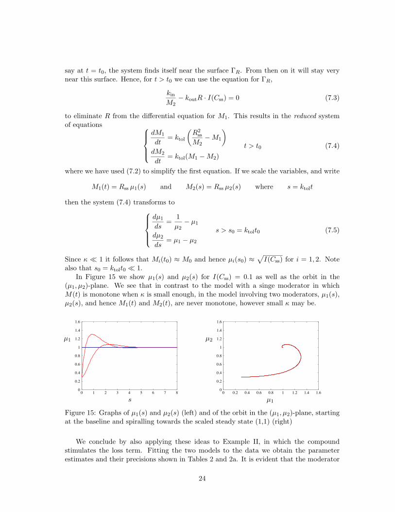
In Figure 15 we show µ1(s) and µ2(s) for I(Css) = 0.1 as well as the orbit in the(µ1, µ2)-plane. We see that in contrast to the model with a singe moderator in whichM(t) is monotone when κ is small enough, in the model involving two moderators, µ1(s),µ2(s), and hence M1(t) and M2(t), are never monotone, however small κ may be.
µ1 µ2
s µ1
0
0.2
0.4
0.6
0.8
1
1.2
1.4
1.6
0 1 2 3 4 5 6 7 80
0.2
0.4
0.6
0.8
1
1.2
1.4
1.6
0 0.2 0.4 0.6 0.8 1 1.2 1.4 1.6
Figure 15: Graphs of µ1(s) and µ2(s) (left) and of the orbit in the (µ1, µ2)-plane, startingat the baseline and spiralling towards the scaled steady state (1,1) (right)
We conclude by also applying these ideas to Example II, in which the compoundstimulates the loss term. Fitting the two models to the data we obtain the parameterestimates and their precisions shown in Tables 2 and 2a. It is evident that the moderator
24

with a transduction compartment model offers a better fit with respect to the goodness-of-fit (cf. Figure 16 left and right) and higher parameter precision.
Table 2: Moderator without transduction
R0 kout ktol kel A n κ1.1 0.17 0.040 0.17 0.0015 3.8 0.25 % 127 % 135 % – 171 % 31% —
Table 2a: Moderator with transduction step
R0 kout ktol kel A n κ1.0 0.23 0.072 0.17 0.0084 3.1 0.32 % 40 % 21 % – 69 % 18 % —
In Figure 16 we show the data and the regression of both models. We see that afterthe overshoot the simpler model predicts that R(t) decreases monotonically to the base-line, whilst in the two-moderator model the regression line shows the oscillatory behaviorpredicted by the mathematical analysis. It is interesting to note that in this examplethe critical parameter κ is not particularly small (κ ≈ 0.3), or different from the originalmodel.
0.0
0.5
1.0
1.5
2.0
0 20 40 60 80 100 120 140 160
Time (min)
0.0
0.5
1.0
1.5
2.0
0 20 40 60 80 100 120 140 160
Time (min)
Original model example II Transduction model example II
Figure 16: Fitting the data set (solid symbols) of Example II with the feedback model(solid line) involving one moderator (left) and a cascade of two moderators (right). Notethe monotone tail on the left and the mildly oscillating tail on the right.
8 Results and Discussion
The Examples I-III capture different properties of the class of models we discuss and therole of the the ratio κ of the two first-order rate constants in the model, kout and ktol:
κ = ktol/kout
In Example I the model captures (i) a steep rise and significant overshoot at the onset ofresponse at the start of the exposure period, (ii) a period over which the response remainsrelatively constant, and (iii) a sharp drop below the baseline (rebound) terminally. Here
25

κ = 1.125. The apparent pharmacodynamic steady-state approaches 3.5 units which issignificantly different from the baseline value.
In Example II the model captures (i) a steep downswing but is lacking any significantovershoot at the onset of response at the start of the exposure period, (ii) a short periodbetween 15 to 30 min over which the response remains relatively constant, and (iii) asharp upswing above the baseline (rebound) post-infusion. There is also a slight tendencytowards oscillatory behavior post-rebound. The two first-order rate constants kout andktol give the characteristics of the response-time course with a κ of 0.235. The apparentpharmacodynamic steady-state approaches 0.25 units, which is significantly less than thebaseline value.
In Example III the model captures (i) a steep rise and the lack of overshoot in exper-imental data at the start of the exposure period, (ii) an extended period of asymptoticdecline of response towards the baseline without rebound, and (iii) two response-timecourses that differs marginally between the two highest doses terminally. The two first-order rate constants kout and ktol give, together with the kinetics of the escitalopram, thecharacteristics of the response-time course with κ of 0.0069. The lack of overshoot andrebound is due to the slow rate constant of the concentration-time data, which confoundsthe former two.
It is timely to say a few words about practical experimental design in relation toparameter identifyability. In order to avoid confounding factors of the system behaviordue to. e.g. slow pharmacokinetics, we suggest step-changes in the plasma concentration.That was demonstrated in particular in Examples I and II. Two or more steady-state levelsof exposure and response may possibly reveal nonlinearities in the concentration-responserelationship (Example III) in that increasing the plasma exposure (increased dose) doesnot necessarily increase response partly due to tolerance. Different rates of drug inputwill trigger different rates and extents of tolerance development. Observations of responsepost-dose (during washout) may reveal different degrees of rebound (Examples I and II)or lack of rebound (Example III).
The proposed feedback models are in principle able to capture large overshoot andlarge rebound with an ”upward bias” in that increasing response versus time curves exhibitlarger tolerance than decreasing response versus time curves (see Figure 17). Specifically,let R0 denote the baseline and Rss the pharmacodynamic steady state. By an upward biaswe mean that
Rss > R0 ⇒ Large overshoot and small reboundRss < R0 ⇒ Small overshoot and large rebound
The ratio κ of the rate constants for the response R (kout) and for the moderator M(ktol):
κ = ktol/kout
is shown to play a critical role in the qualitative properties of the models. In the extremecase, when κ+ 1, precise estimates can be given for overshoot and rebound.
It is demonstrated how in state space, i.e., the (R,M)-plane, shown in Figure 17, prop-erties, such as upward bias and dependence on the ratio κ = ktol/kout, can be explained by
26

simple geometric arguments. The curvature of the null cline ΓR, which serves as a boundfor the response (since dR/dt = 0 on ΓR) creates more room for an upswing (gain) andless room for a down swing (loss).
R
M loose
gain
Figure 17: The upward bias: Schematic sketch of the phase plane with two nullclines, onefor C = 0 (lower hyperbola) and one for C = Css > 0 (upper hyperbola). In the extremecase of very small ktol, Rmax can gain at the overshoot and loose at the rebound, asindicated by the thick line segments
Many other qualitative properties of the two feedback models are established, often bygeometrical methods. We mention in particular: after the onset of a constant rate infusionwhich extends for a sufficiently long time T , the maximal response Rmax occurs at thefirst local maximum, at Tmax, of the response versus time graph.
We exibit the profound effect of κ on the size of overshoot and rebound, in particularfor κ + 1 and for κ , 1, and we touch on the question of the effect of the plasmaconcentration versus time profile C(t) on the size of overshoot and rebound.
During the analysis with the basic feedback model we have encountered two new sit-uations, the multiple moderator or transduction model and the trigger phenomena, forwhich we propose tentative explanations.
In light of the three examples, the qualitative analysis, the identifiability discussionand the two extensions, we believe that from our perspective the basic feedback systemconstitutes a flexible class of models that captures all kinds of features commonly observedin tolerant systems.
Appendices
A Dimensionless variables
In order to isolate the parameters that really determine the dynamics of the system (3.1), itis useful to transform to dimensionless variables. Natural reference values for the response
27

R and the moderator M are their baseline values. Thus, we put
R(t) = R0y(t), M(t) = M0x(t), R0 = M0 =√
kin
kout(A.1)
This yields the following system of equations
dy
dt= kout
{1x− y ·H (C(t))
}and
dx
dt= ktol(y − x) (A.2)
The rate constant of the dimensionless response y at the baseline, when H(C) = 1, isgiven by kout. Therefore, a natural unit of time will be t0 = 1/kout. Thus, scaling thetime with t0 yields the dimensionless time τ = t/t0. When we introduce this time into thesystem (A.2) and write
y∗(τ) = y(t), x∗(τ) = x(t), C∗(τ) = C(t)
and omit the asterisks again, we obtain the dimensionless system
dy
dτ=
1x− y ·H (C(τ))
dx
dτ= κ(y − x) where κ =
ktol
kout
(A.3)
Thus, we find that qualitatively, the dynamics of the system (3.1) is determined by onlyone parameter, κ, and of course by the forcing function H(C(τ)).
When the concentration C is frozen, say at Css, then the equilibrium points are givenby:
xss = yss =1√
H(Css)(A.4)
By design, at the baseline, when C = 0 and H(0) = 1, we have (xss, yss) = (1, 1).
B Proof of basic properties
In proving basic properties of the system (A.3) we use the phase plane as introduced inSection 3 and view the pair of functions (x(τ), y(τ)) as a point tracing out an orbit γ inthe (x, y)-plane:
γ = {(x(τ), y(τ)) : 0 ≤ τ <∞} (B.1)
Standard ODE theory [3] states that if C is frozen, then through each point (x, y) (x .= 0),passes precisely one orbit. This means, in particular, that orbits cannot self-intersect.Throughout this Appendix we assume that
C(τ) = Css ≥ 0 for τ > 0; C(0) = 0 (B.2)
Also, throughout we consider the inhibitory case, H(C) = I(C). The case when the lossterm is stimulated is similar.
28

The direction and the speed with which the orbit passes through (x, y) is given bythe velocity vector v = (dx/dτ, dy/dτ) evaluated at (x, y). If we write v = (vx, vy), then,according to the system (A.3),
vy =1x− y · I(Css) and vx = κ(x− y) (B.3)
The null clines are the curves Γx and Γy on which the vector v is parallel to, respectively,the y-axis (vx = 0) and the x-axis (vy = 0). By (B.3) these curves are given by
Γy ={
(x, y) :1x− y · I(Css) = 0
}and Γx = {(x, y) : x− y = 0} (B.4)
At points where Γx and Γy intersect we have dx/dτ = 0 as well as dy/dτ = 0. Therefore,these points are equilibrium points.
In Figure 18 we show four orbits in the phase plane for κ = 1 and Css = 0. They startat the points (x, y) = (0.1, 0.1), (0.2, 0.2), (0.3, 0.3) and (0.4,0.4). We have also includedthe two null clines for Css = 0. We see that where the orbits cross Γy the tangents to theorbits are horizontal and that on Γx the tangents to the orbits are vertical.
0 0.5 1 1.50
0.5
1
1.5
2
2.5
y
x
Figure 18: Four orbits of (A.3) starting at (x, y)(0) = (0.n, 0.n), n = 1, 2, 3, 4 when κ = 0.5and Css = 0, as well as the corresponding null clines Γy and Γx (dashed)
We begin by proving upper and lower bounds for y(t) and x(t) which are valid for allτ > 0.
Theorem B.1 Suppose that C(τ) is given by (B.2) in which Css > 0, and let (x(τ), y(τ))be the solution of (A.3), with H(C) = I(C), which starts at the baseline, i.e., (x, y)(0) =(1, 1). Then
1 < y(τ) <1
I(Css)and 1 < x(τ) <
1I(Css)
for τ > 0 (B.5)
Proof. We define the following box in the phase plane (see Figure 19):
B = {(x, y) : 1 < x < 1/I(Css), 1 < y < 1/I(Css)}
29

At t = 0, the orbit starts from the the baseline point (1,1) i.e., from the lower left cornerof the box. By the system of equations (A.3) we have
dy
dτ= 1− I(Css) > 0 and
dx
dτ= 0,
d2x
dτ2= κ
dy
dτ> 0 at τ = 0+
Therefore, the orbit curves into B1 and hence, for small τ > 0 the orbit lies in the box B.The theorem will be proved if we show that the orbit remains in the box for all τ > 0.
Inspection of the velocity vector v reveals that everywhere on the boundary of B,except at the corners, v points into B. Therefore, the orbit can never leave B throughone of its sides. It is readily seen that the orbit can never reach one of the corners, so thatwe may conclude that (x(τ), y(τ)) ∈ B for all τ > 0. !
In the next theorem we show that the state of the system converges to the pharmaco-dynamic steady state.
Theorem B.2 Suppose that C(τ) is given by (B.2) in which Css > 0, and let (x(τ), y(τ))be the solution of (A.3), with H(C) = I(C), which starts at the baseline, i.e., (x, y)(0) =(1, 1). Then
x(t)→ xss and y(t)→ yss as t→∞
Proof. We now follow the orbit as it enters the box B form the baseline point (1,1). Itwill be convenient to divide B into four parts, separated by the null clines:
B1 : (x, y) lies above Γx and below Γy
B2 : (x, y) lies above Γx and above Γy
B3 : (x, y) lies below Γx and above Γy
B4 : (x, y) lies below Γx and below Γy
The regions B1, . . . ,B4 are shown in Figure 19.
! x!y
B1
B2
B3
B4
B
x
y
Figure 19: The box B and the subdomains B1, . . . ,B4 in the (x, y)-plane
Plainly, the orbit first enters the region B1. There are now two possibilities: eitherthe orbit remains in B1 for all τ > 0, or it leaves B1 in finite time, say at τ1. The first
30

possibility implies that both x(τ) and y(τ) are inceasing for all τ > 0. Since they arebounded above, they must tend to a limit, i.e., the orbit must tend to a stationary point.This can only be (xss, yss), and the theorem is proved.
Thus, let us assume that the orbit leaves B1 at τ1 > 0. This can only happen throughΓy, so that the orbit enters B2. Again, we have the same two possibilities. If the orbitstays in B2 the theorem is proved, and so we assume that it leaves B2 through Γx andenters B3. Repeating this argument we find that eventually, the orbit is back in B1, inthe region below the segment of the orbit for 0 < τ < τ1. Continuing this process we findthat, either after a finite time the orbit remains in one of the four subsets of B, or it spiralstowards a periodic orbit or towards the point (xss, yss).
By means of Dulac’s test [8] one can show that this system cannot have a periodicsolution. Therefore the orbit must spiral towards the point (xss, yss) and the theorem isproved. !Remark Theorem B.2 continues to hold if (x(0), y(0)) = (x0, y0) and (x0, y0) is anarbitrary point in the first quadrant.
It is evident from the spiralling character of the orbit that the intersection of theorbit with B1 is a decreasing sequence of curves, whose intersections with Γy will also bedecreasing. This observation yields the following result:
Corollary B.1 If an orbit intersects Γy, then the first time this happens will be at τ =τmax and ymax = y(τmax).
Theorem B.1 yields uniform bounds for x(τ) and y(τ). In the following theorem weuse the lower bound for x(τ) to improve on the upper bound for y(τ). Let y(τ) be thesolution of the problem
dy
dτ= 1− y · I(Css), y(0) = 1 (B.6)
in which the equation is the dimensionless version of equation (3.9).
Theorem B.3 Suppose that C(τ) is given by (B.2) in which Css > 0, and let (x(τ), y(τ))be the solution of (A.3), with H(C) = I(C), which starts at the baseline, i.e., (x, y)(0) =(1, 1). Then
y(τ) < y(τ) =1
I(Css)
{1− [1− I(Css)]e−τI(Css)
}for τ > 0 (B.7)
Proof. We subtract the equation for y(τ) from the equation for y(τ) and write z(τ) =y(τ)− y(τ). Then
dz
dτ= 1− 1
x− z · I(Css) > −z · I(Css) for τ > 0
because, by Theorem B.1, x(τ) > 1 for all τ > 0. This means that
d
dτ(eτI(Css)z) = eτI(Css)
(dz
dτ+ z · I(Css)
)> 0 for τ > 0 (B.8)
31

If we now integrate (B.8) over (0, τ) and use the initial condition z(0) = 0, we find that
eτI(Css)z(τ) > 0 for τ > 0
and hence thatz(τ) = y(τ)− y(τ) > 0 for τ > 0
as asserted. !We conclude with a few observations about the influence of κ. We begin with a general
monotonicity property which is demonstrated in Figure 20
Γ1
Γ2
Γ3
0
1
2
3
4
5
6y
0 0.5 1 1.5 2 2.5 3 3.5x
Figure 20: Orbits Γ1,2,3 of (A.3) for, respectively, κ1 = 0.01, κ2 = 0.04 and κ3 = 0.1 andI(Css) = 0.15
Theorem B.4 Suppose that C(τ) is given by (B.2) in which Css > 0, and let (xi(τ), yi(τ))(i = 1, 2) be solutions of (A.3), with H(C) = I(C), which start at the baseline, i.e.,(xi, yi)(0) = (1, 1) and correspond to, respectively, κ1 and κ2. Let Γ1 and Γ2 be theintersections of the corresponding orbits with B1. Then
κ1 < κ2 =⇒ Γ1 lies above Γ2 in B1 (B.9)
Proof. Consider the region Q in B1 which is bounded below by Γ2 and above by Γy (cf.Figure 19). Observe that
d2xi
dτ2= κi
dyi
dτ= κi {1− I(Css)} at τ = 0+
Hence, if κ1 < κ2, thend2x1
dτ2<
d2x2
dτ2at τ = 0+
so that the orbit Γ1 enters the region Q. It is readily seen that if κ = κ1, the vector fieldv points into Q along the line {x = 1} as well as along Γ2. Hence, Γ1 will remain in Quntil it leaves through Γy. !
32

We conclude with an analysis of the manner in which the orbit approaches the steadystate (xss, yss), under an angle or in a spiral. This is done by linearizing the system (A.3)about (xss, yss). We thus obtain the linear system u′ = Au, in which
A =(−I(C) −x−2
ss
κ −κ
)and u =
(yx
)(B.10)
The eigenalues λ± of the matrix A are the roots of the equation
λ2 + {I(C) + κ}λ + 2κI = 0
They are given by
λ± = −12{I(C) + κ} ± 1
2√{I(C) + κ}2 − 8κI(C) (B.11)
They are real-valued if the discriminant D = {I(C) + κ}2 − 8κI(C) is nonnegative. Thisis readily seen to be the case when
κ ≤ κ− or κ ≥ κ+, where κ± = (3± 2√
2)I(C) (B.12)
Plainly, the real value of both eigenvalues is always negative, so that, consistent withTheorem B.2, (xss, yss) is always locally stable. We distinguish two cases:(a) κ− < κ < κ+: The orbit spirals into (xss, yss) , and(b) κ < κ− or κ > κ+: The orbit enters (xss, yss) from certain, well specified, directions.These directions are given by the eigenvectors q± of the matrix A:
q± = (q±y , q±x ) where q±y = κ + λ±, q±x = κ.
An elementary computation shows that
q±y < 0 if κ < κ− and q±y > 0 if κ > κ+
Since q±x > 0 for all κ > 0, this implies that if κ < κ−, then q+ and q− point into thefourth quadrant and if κ > κ+, then q+ and q− point into the first quadrant.
Thus, for κ < κ+ there will be overshoot.
Remark For the data used in Figure 20 we have κ− = 0.0257 . . . and κ+ = 0.874 . . . .Therefore, κ1 < κ− and κ− < κ2,κ3 < κ+, which is consistent with the behavior of theorbits near (xss, yss) shown in Figure 20.
References
[1] E. Ackerman, J.W. Rosevear and W.F. McGuckin. A mathematical model oftheglucose-tolerance test, Phys. Med. Biol. 9:203-213 (1964).
[2] J.A. Bauer, and H.L. Fung. Pharmacodynamic models of nitroglycerin-induced hemo-dynamic tolerance in experimental heart failure. Pharm.Res. 11:816-823 (1994).
[3] P. Blanchard, R. L. Devaney and G.R. Hall, Differential Equations, Brooks/ColePublishing C, Pacific Grove, CA, 1998.
33

[4] C. Bundgaard, F. Larsen, Martin Jorgensen and J. Gabrielsson, Mechanistic turnovermodel including autoinhibitory feedback regulation of acute 5-HT release in ratbrain after administration of selective serotonoin reuptake inhibitors (SSRI’s), Eur.J. Pharm. Sci. (in press 2006).
[5] W.A. Colburn and M.A. Eldon, Simultaneous pharmacokinetic/Pharmacodynamicmodeling. In: Pharmacodynamics and drug development: Perspectives in clinicalpharmacology. Ed. N.R. Butler, J.J. Sramek and P.K. Narang. Wiley, New York(1994).
[6] J. Gabrielsson and D. Weiner, Pharmacokinetic and pharmacodynamic data analy-sis: Concepts and applications, 4th Ed., Swedich Pharmaceutical Press, Stockholm,(2006).
[7] N.H.G. Holford, J. Gabrielsson, L.B. Sheiner, N. Benowitz and R. Jones. A physiolog-ical pharmacodynamic model for tolerance to cocaine effects on systolic blood pressure,heart rate and euphoria in human volunteers, Poster at Measurement and Kinetics ofIn Vivo Drug Effects: Advances in simultaneous pharmacokinetic/pharmacodynamicmodelling, Noordwijk, The Netherlands, 28-30 June, 1990.
[8] D.W. Jordan and P. Smith, Nonlinear Ordinary Differential Equations, ClarendonPress, Oxford, 1977.
[9] C.H. Kleinbloesem, P. van Brummelen, P. van de Linde, J.A. Voogd and D.D.Breimer, Nifedipine: kinetics and dynamics in healthy subjects, Clin. Pharmacol.Ther. 35:742-749 (1984).
[10] C.H. Kleinbloesem, J. van Harten, L.G.J. de Leede, P. van Brummelen and D.D.Breimer, Kinitics and hemodynamics of nifedipine:in during rectal infusion to steadystate with osmotic system, Clin. Pharmacol. Ther. 36:396-401 (1984).
[11] C.H. Kleinbloesem, P. van Brummelen, M. Danhof, H. Faber, J. Urquhart and D.D.Breimer, Rate of increase in the plasma concentration of nifedipine as a major deter-minant of its hematodynamic effects in humans, Clin. Pharmacol. Ther. 41: 26-30(1987).
[12] W. Krzyzanski and W.J. Jusko, Mathematical formalism for the properties of fourbasic models of indirect pharmacodynamic responses. J. Pharmacokin. Biopharm.25:107-123 (1997).
[13] W. Krzyzanski and W.J. Jusko, Mathematical formalism and characteristics of fourbasic models of indirect pharmacodynamic responses for drug infusions. J. Pharma-cokin. Biopharm. 26:385-408 (1998).
[14] V. Licko, and E.B. Ekblad. Dynamics of a metabolic system: what single-action agentsreveal about acid secretion. Am. J. Physiol. Gastrointest. Liver Physiol. 262:G581-G592 (1992).
[15] L.A. Peletier, J. Gabrielsson and J. den Haag, A Dynamical Systems Analysis of theIndirect Response Model with Special Emphasis on Time to Peak Response, Journalof Pharmacokinetics and Pharmacodynamics, 32:607-654 (2005).
[16] V. Peng-Pederson and N.B. Modi, A system approach to pharmacodynamics. Input-effect control system analysis of central nervous system effect of alfentanil, J. Pharm.Sci. 82:266-272 (1993).
34

[17] A. Sharma, W.F. Ebling and W.J. Jusko. Precursor-Dependent Indirect Pharmaco-dynamic Response Model for Tolerance and Rebound Phenomena, J. PharmaceuticalSciences 87:1577-1584.
[18] J. Urquhart, and C.C. Li, Dynamic testing and modeling of andrecortical secretoryfunction, Ann. NY Acad. Sci. 156:756-778 (1969).
[19] J. Urquhart, and C.C. Li, The dynamics of adrenocortical secretion, Am. J. Physiol.214:73-85 (1968).
[20] J. Urquhart, History-Informed Perspectives on the Modeling and Simulation of Ther-apeutic Drug Actions. In Simulations for Designing Clinical Tryals, Edited by HuiC. Kimko and Stephen B. Duffull, Marcel Dekker, 2002.
[21] M. Wakelkamp, G. Alvan, J. Gabrielsson and G. Paintaud, Pharmacodynamic mod-eling of furosemide tolerance after multiple intravenous administration, Clin. Phar-macol. Ther. 60:75–88 (1996).
[22] K.P. Zuideveld, H.J. Maas, N. Treijtel, J. Hulshof, P.H. van der Graaf, L.A. Peletier,and M. Danhof. A set-point model with oscillatory behaviour predicts the time courseof 8-OH-DPAT-induced hypothermia. Am. J. Physiol. Regul. Integr. Comp. Physiol.281:R2059-R2071(2001).
35