A Non-Technical Introductionto Hazard Rate Analysis

DIMETIC SessionRegional Innovation Systems, Clusters, and Dynamics

Maastricht, October 8-12, 2007

Guido BuenstorfMax Planck Institute of Economics

Evolutionary Economics Group

What survival analysis originally WAS about:Drug testing:• 48 subjects in test

• 28 take the drug to be tested; 20 take a placebo

• Information at end of study:• Subject still alive?

• If not, when did they die?

Survival analysis analysis of• Incidence of event (0/1)

• Time t to event

Dependent variable: ”risk” (hazard rate)

0,000P > chi2

-83,324Log-Likelihood

48(31)

Observations(Event = 1)

0,114***(0,042)

Age

-1,226***(0,347)

Drug

Model1 (Cox Regression)

Standard error in parentheses; ***p≤ 0,01; **p≤ 0,05; *p≤ 0,10

Hazard rate analysis: overview

Hazard rate analysis• = survival analysis; duration analysis

• Origins in medical statistics; demographics; engineering

• Is applied to handle duration data applicable in many economic contexts

• Requires frequently repeated (better: continuous) observations of subjects

• Uses maximum likelihood estimations

• Is implemented in standard statistical software

Hazard rate analysis: literature

Some introductory reading:• Overview article on HRA:

• Kiefer (JEL, 1988)

• How-to book on HRA using STATA:

• Cleves/Gould/Gutierrez: An Introduction to Survival Analysis UsingStata, College Station TX: Stata Press, 2002.

• Competing risks models:

• Lunn and McNeil (Biometrics, 1995)

• Bogges (2004) :Implementation in STATA: http://www.stata.com/statalist/archive/2004-05/msg00506.html

• Discrete-time models:

• Jenkins (Oxford Bulletin of Economics and Statistics, 1995)

Applications (1): Firm survival

Widely used in empirical industry evolution / organization ecology literature

Longevity as proxy for performance

Analogous situation to drug testing example:• Firm still active at end of study?

• If not, how long were they active?

• Complication: exit for non-performance-related reasons (acquisition)

Most frequently studied:• Time of entry and survival

• Pre-entry experience and survival

• “Density-dependence” (aggregate; local) time-varying covariates

Example: Firm survival in 4 U.S. industries

-178.674-486.354-1773.015-1948.312Log-likelihood

-2.342***(.215)

-1.676***(.123)

-1.603***(.069)

-1.619***(.060)

Constant

-.003(.014)

-.024**(.012)

-.041***(.005)

-.025***(.005)

Firm age

-.344***(.102)

-.073(.094)

Entrycohort 3

-.561***(.182)

-.529***(.117)

-.392***(.115)

Entrycohort 2

-1.042***(.337)

-1.173***(.286)

-.461***(.152)

-.478***(.138)

Entrycohort 1

Penicillin(1943-1992)

TVs(1946-1990)

Tires(1905-1980)

Autos(1895-1966)

Source: Klepper (RAND Journal, 2002)The group of most recent entrants is the omitted control group in each model. Gompertz specification; standard errors in parentheses; ***p≤ 0,01; **p≤ 0,05; *p≤ 0,10

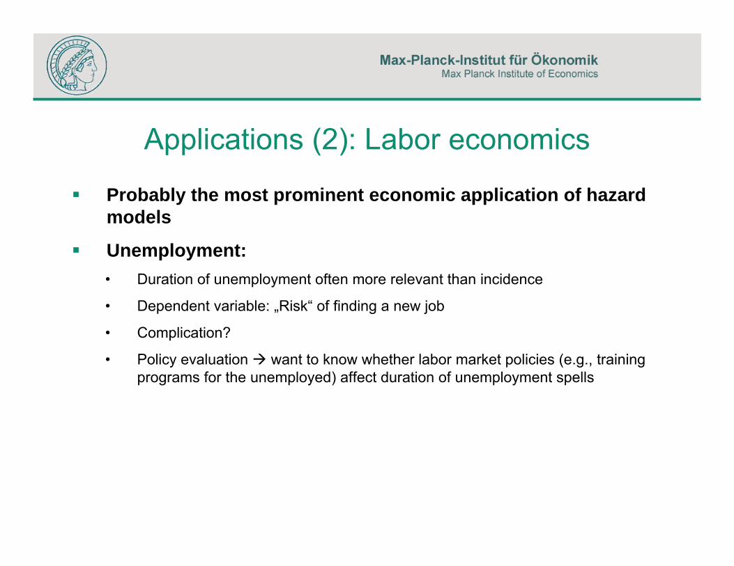
Applications (2): Labor economics

Probably the most prominent economic application of hazardmodels

Unemployment:• Duration of unemployment often more relevant than incidence

• Dependent variable: „Risk“ of finding a new job

• Complication?

• Policy evaluation want to know whether labor market policies (e.g., training programs for the unemployed) affect duration of unemployment spells

Applications (3): Technology transfer

Example: commercialization of licensed university technology

Issue: Characteristics of licensees• Inventor startups more or less likely to commercialize than established

firms?

• Hazard rate analysis accounts for:

• Time to commercialization

• Non-commercialization at end of study (“censoring”)

Message from applications

Hazard rate analysis (HRA) has many applications

„Survival“ need not be good; „risk“ need not be bad

HRA measures both occurrence of event and time lapsed before the event…

… and can account for artificially imposed end of duration („censoring“)

Why does HRA need special methods?

Reason 1: Characteristics of duration data• Durations are never negative

• Durations are frequently not normally distributed ( “bathtub hazard” of human mortality)

Reason 2: Censoring and truncation of observations • („End-of-observation-for-reasons-other-than-what-we-are-interested-in“)

Key concepts (1)Failure• Event of interest that terminates the period of risk for a given subject

Conditional probability of failure • Probability of failure conditional on not having failed before (analogy to

sports tournament)

Hazard function ( instantaneous rate of failure)• Conditional failure probability over infinitesimally small time period

Origin• Time at which the risk begins often differs between subjects

Spell• Total time that a given subject is at risk

Key concepts (2)Some definitions: (T: time of failure)

• Probability distribution of duration: F(t) = Pr(T < t) (density f(t) = dF(t) / dt))

• Survivor function: S(t) = 1 – F(t) = Pr(T ≥ t)

• Hazard function: h(t) = f(t) / S(t)

Note: hazard rate equals absolute slope of logarithmic survivor function:

[ ] [ ]dt

tSddt

tFddt

tFdtFtF

tftStfth )(ln)(1ln)(1

)(11

)(1)(

)()()( −=

−−=

−

−−=

−

−−==

Censoring (1)Two causes of censored observations:

• Exit for reasons unrelated to interest of study• Industry evolution: exit by acquisition (Chrysler vs. Skype)

• Labor economics: unemployment spell ends because individual reaches pension age (or is hit by train)

• Imperfections in study design / available data• Right censoring (pervasive): not all individuals have exited at end of study

• Left censoring: begin of spell is unknown

• Length-based censoring:

– Entry and exit unobserved because both fall into same time span between two observations

– Exit falls into interval between two observationstied failures: order of individuals’ failures cannot be established

• Failure before begin of study no observations exist (if absorptive failure)

Censoring (2)Statistical treatment of (right) censored observations:

(intuition only, see Kiefer (JEL, 1988) for technical details)

• Survival analysis based on maximum likelihood estimations

• Uncensored exits contribute exit density fi(t)

• Censored exits contribute survivor function Si(t)

Only information that they survived up to t enters the likelihood function

TruncationNo information about events and covariates for some time

Relevant: Left truncation (delayed entry): • Individual enters risk before first observation

• For example, no systematic information may exist for first years of an industry, but founding dates of surviving firms are known

• Observing the firm implies that no failure before beginning of study

• Can be handled by STATA by distinguishing entry from origin

• However, doing so means that we no longer study full population (some may have failed before first observation)

Three classes of methods

Non-parametric analysis• No assumptions on functional forms “data speak for themselves”

• Most important: Kaplan-Meier estimator

Semi-parametric analysis• Functional form specified for:

• effects of covariates on hazard rate

(Fully) parametric analysis• Functional form specified for:

• effects of covariates on hazard rate

• distribution of failure times

Kaplan-Meier estimator (1)

Non-parametric estimate of survivor function S(t)

where• tj (j = 1..K): observed time of failures

• nj: number of individuals at risk at time j

• dj: number of failures at time j

Notes:• Applicable only to categorical covariates

• Censoring: STATA convention: at time t, failures occur before censoring (i.e., censored observations are in risk set at t)

• If survival probabilities on logarithmic scale: (absolute) slope = hazard rate

( ) ∏≤

⎟⎟

⎠

⎞

⎜⎜

⎝

⎛ −=

ttj j

jj

jn

dntS

Kaplan-Meier estimator (2)

Let’s do some practical econometrics – no computer required!

Approach:1. Order cases by covariate values and survival times (shortest one first)

2. Calculate (nj – dj) / nj

3. Calculate running product

Of course, Kaplan-Meier estimator also implemented in statistical software…

Kaplan-Meier estimator (3)0.

000.

250.

500.

751.

00

0 20 40 60 80analysis time

diversifier spin-offstartup

Kaplan-Meier survival estimates, by background

The proportional hazards assumptionRelevant to both semi-parametric and fully parametric models• Covariates’ effect is to multiply hazard function by a scale factor

h0: “baseline hazard”

effect of explanatory variables does not depend on duration

baseline hazard has same shape for all values of covariates

quite heroic assumption in many applications !

• Because of non-negativity constraints, exponential is normally used

Simple check of proportionality assumption: • If hazards are proportional, log-scale Kaplan-Meier graphs are parallel for

different groups

Real tests exist and should be used ( Schoenfeld residuals)

),()(),,,( 00 ββ xthhtxh Φ=

)exp()(),,,( 00 ββ xthhtxh ′=

Cox proportional hazards model (1)Semi-parametric model: no assumptions on functional form of baseline hazard

But: assumption that baseline hazard has same shape for all individuals may be problematic

In essence, Cox model is sequence of conditional logits• Data ordered by times of failures (similar to Kaplan-Meier)

• Coefficients are estimated such that at each time of failure tj, the likelihood is maximized that the failing individual is the one that actually failed (among the individuals still at risk at tj)

Coefficient estimates driven by order of failure (ties are handled by specific procedures)

Cox proportional hazards model (2)

Shortcoming: information of time intervals between the failures is not used

Likely to affect outcomes if intervals differ strongly

Also: inefficient because not all information in data is used

Fully parametric proportional hazards models (1)Key difference to Cox model: assumptions on functional form of baseline hazard h0

Crucial issue: Do we have reasonable priors on age-dependence of hazards ( theory)?

Firm survival: “liability of newness”; “liability of senescence” decreasing or U-shaped age-dependence

Most frequently used distributions:• Exponential: h0(t) = exp(a) constant baseline hazard

• Weibull: h0(t) = p tp-1 exp(a) reduces to exponential for p=1

• Gompertz: h0(t) = exp(a) exp(γt)

Fully parametric proportional hazards models (2)

Relaxing the proportional hazards assumption

Is straightforward for fully parametric estimators

Example: • Different age-dependent effects for different entry cohorts; backgrounds

• Interpretation: dynamics of performance may differ between groups

• Possible explanation: selection effects; composition of cohorts varies over time, as lesser performers are weeded out

Baseline hazard of fully parameterized Gompertz model:

[ ]tzth )(exp)( 00 γγ ′+=

ExtensionsDiscrete time models• Different conventions regarding acceptability of continuous time models

• With yearly data and short spells discrete time models should be considered

• Literature: Jenkins, 1995

Competing risks• Allows consideration of two (or more) kinds of events (e.g., bankruptcy versus

acquisition)

• Implementation is straightforward

Time-varying covariates• Spells are broken into shorter time periods (e.g., years)

• STATA can handle multiple observations per subject

• Current values of covariates are used for each individual observation