a non-oscillatory no-free-parameter finite element and its applications in cdf

INTERNATIONAL JOURNAL FOR NUMERICAL METHODS IN FLUIDS, VOL. 24, 141–153 (1997)

A NON-OSCILLATORY NO-FREE-PARAMETER FINITEELEMENT ALGORITHM AND ITS APPLICATIONS IN CFD

YAN WANG AND BING-GANG TONGGraduate School, University of Science and Technology of China, PO Box 3908, Beijing 100039, People’s Republic of China

AND

GUI-QING JIANG AND XIAO-MIN WANGBeijing Institute of Aerodynamics, PO Box 7215, Beijing 100074, People’s Republic of China

SUMMARY

A non-oscillatory no-free-parameter finite element method (NNFEM) is presented based on the consideration ofwave propagation characteristic in different characteristic directions across a strong discontinuity through fluxvector splitting in order to satisfy the increasing entropy condition. The algorithm is analysed in detail for theone-dimensional (1D) Euler equation and then extended to the 2D, axisymmetric and 3D Euler and Navier–Stokes equations. Its applications in various cases—inviscid oblique shock wave reflection, flow over a forwardstep, axisymmetric free jet flow, supersonic flows over 2D and 3D rectangular cavities—are given. Thesecomputational results show that the present NNFEM is efficient in practice and stable in operations and isespecially capable of giving good resolution in simulating complicated separated and vortical flows interactingwith shock waves.

KEY WORDS: finite element; non-oscillatory; strong discontinuity

1. INTRODUCTION

The development of the finite element technique and its extensive applications in CFD has attractedmore and more researchers in recent decades. One of its main difficulties is how to get high-resolution computations in shock wave regions and also in complicated viscous flow fields. Incomparison with the success of high-resolution finite difference schemes such as TVD1 and NND,2

some advances have been achieved in finite element algorithms. The streamline upwind Petrov–Galerkin (SUPG) algorithm of Hughes and Mallet3 and the ENO discretized algorithm of Baker andKim4 can eliminate the spurious oscillations in simulating shock waves, but their computationalresolution across shock waves is still unsatisfactory. Remakrishmanet al.5 increased thecomputational resolution in the shock wave region by adding artificial viscosity in the discretizationand using the mesh refinement or mesh self-adaptation technique, but were not very successful inpractice and still worried about the existence of spurious oscillations. The failure of the finite elementmethod in this respect seriously retards its ability to successfully simulate complex super-sonic=hypersonic flow problems.

Referring to an idea used in the finite difference method,2 we propose here a non-oscillatory no-free parameter finite element method (NNFEM) based on the consideration of wave propagation

CCC 0271–2091/97/020141–13 Received August 1995# 1997 by John Wiley & Sons, Ltd. Revised March 1996

characteristic in different characteristic directions across a strong discontinuity through flux vectorsplitting in order to satisfy the increasing entropy condition. For verification of the present algorithman inviscid oblique shock wave reflection and a supersonic flow over a forward step are computed andcompared with available results. Also, an axisymmetric free jet flow with a high pressure ratio iscomputed, where a Mach disc and a drum-like shock wave have been clearly shown. Next, supersonicflows over 2D and 3D rectangular cavities are successfully simulated, where periodic motions ofshock waves and vortex flows have been investigated.

In Section 2, we introduce the present algorithm in the discretization of the 1D Euler equation. Thenit is extended to discretize the 2D, axisymmetric and 3D Euler equations in Section 3. In Section 4several applications and discussions are given. Finally, conclusions are presented in Section 5.

2. NNFEM IN DISCRETIZATION OF 1D EULER EQUATIONS

The 1D Euler equation has the form

@U

@t�

@F

@x� 0;

U �

r

rue

2

4

3

5; F �

ruru2

� p�e � p�u

2

4

3

5;

�1�

whereu; r; p and e denote velocity, density, pressure and total specific energy respectively. Nowequation (1) can be discretized by the Galerkin weighted residual method and integrated usingGreen’s formula. For every elemente we have

�

e�N ��N �

T dx@u

@t

� �

�

�

e

@�N �

@xF dx � boundary conditions: �2�

Figure 1. 2D element co-ordinate transformation

Figure 2. 3D element co-ordinate transformation

142 Y. WANG ET AL.

In the classic Galerkin finite element method, the flux vectorF is approximated linearly as

F � NiFi � NjFj;

Ni � �xj ÿ x�=�xj ÿ xi�; Nj � �x ÿ xi�=�xj ÿ xi�;

where i and j denote the nodes of the elemente. This expression leads to the spurious oscillationsacross a strong discontinuity, otherwise an artificial viscosity is needed.

Now we attack the problem physically. First, according to the different characteristic directions,F is split by Steger’s technique6 into positive and negative fluxes so that the following hold.

(i) F � AU , i.e. F is a homogeneous function ofU.(ii) The Jacobian matrixA may be written as

A � @F=@U � Sÿ1LS;

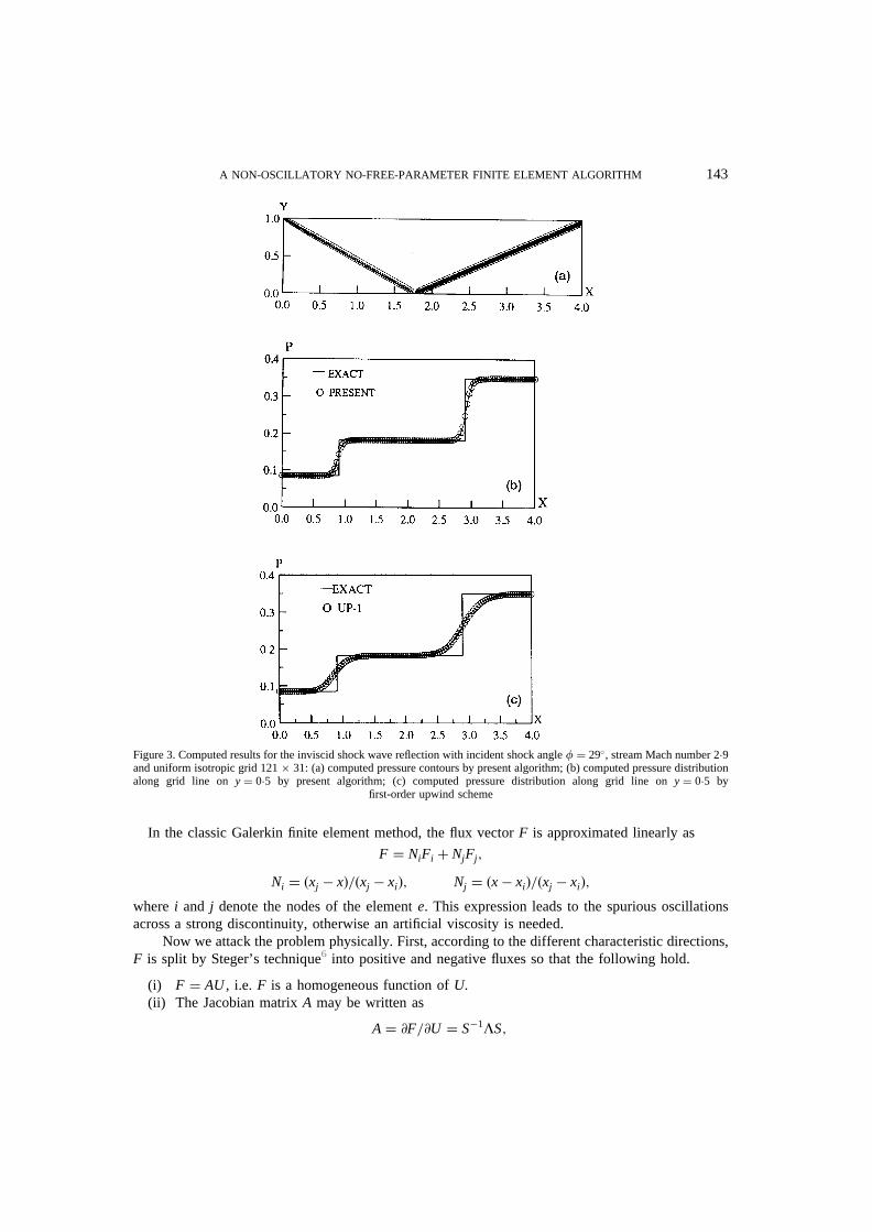
Figure 3. Computed results for the inviscid shock wave reflection with incident shock anglef � 29�, stream Mach number 2�9and uniform isotropic grid 121631: (a) computed pressure contours by present algorithm; (b) computed pressure distributionalong grid line on y � 0�5 by present algorithm; (c) computed pressure distribution along grid line ony � 0�5 by

first-order upwind scheme

A NON-OSCILLATORY NO-FREE-PARAMETER FINITE ELEMENT ALGORITHM 143

whereS is a non-singular characteristic vector. Ifli denote the characteristic roots ofA, then

L � diagflig; i � 1; 2; 3:

(iii) By using Steger’s splitting technique,

L�

� diagli � jlij

2

� �

; i � 1; 2; 3:

(iv) We getF�

� Sÿ1L

�SU � A�U ; F � F�

� Fÿ

:

Up to now it is clear that forF� the waves propagate from the upstream to the downstream andreversely forFÿ. We can simulate this by using the forward and backward finite difference technique.HenceF� and Fÿ in the elemente may be expressed with forward and backward Taylor seriesexpansions respectively up to second-order accuracy as

F�

e �x� � F�

i � �x ÿ xi�@F�

@x

� �

i

� O�Dx2�; Fÿ

e �x� � Fÿ

i � �x ÿ xj�@Fÿ

@x

� �

j

� O�Dx2�; �3�

@F�

@x

� �

i

�

F�

j ÿ F�

i

Dx� O�Dx�;

@Fÿ

@x

� �

j

�

Fÿ

j ÿ Fÿ

i

Dx� O�Dx�: �4�

In order to eliminate spurious oscillations across the shock wave, according to the analysis madefor the construction of the NND scheme,2 each derivative in (3) should be taken to be one, whichabsolute value is the minimum between those on nodesi and j. If the signs of these derivatives oniand j are different, we just take the minimum value to be zero. If the symbolminmod is used, i.e.

minmod�a; b� � 0�5 �sign�a� � sign�b��min�jaj; jbj�;

Figure 4. Density contours of 2D forward step

Figure 5. Pressure distribution along wall for 2D forward step

144 Y. WANG ET AL.

then

@F�

@x

� �

im

� minmod@F�

@x

� �

i

;

@F�

@x

� �

j

" #

;

@Fÿ

@x

� �

jm

� minmod@Fÿ

@x

� �

i

;

@Fÿ

@x

� �

j

" #

: �5�

Finally the expression ofF is given as

F � F�

i � Fÿ

j � �x ÿ xi�@F�

@x

� �

im

� �x ÿ xj�@Fÿ

@x

� �

jm

: �6�

Substituting (6) into (2), we get the present discretized finite element algorithm which is accurate tosecond order.

For the N–S equation the viscous term and the source term may still be discretized by theclassical Galerkin finite element method.

It can be proven that if the mass matrix of the left-hand term of (2) is replaced by a lumpeddiagonal mass matrix,7 the present algorithm is reduced to the same form as the NND scheme.

Figure 6. (a) Density and (b) pressure contours in analysis of inviscid free jet flow with uniform isotropic grid 61661

Figure 7. Mach number distribution along centreline of inviscid free jet flow


3. EXTENSION OF NNFEM TO MULTIDIMENSIONAL EULER EQUATIONS

3.1. Discretization of 2D and axisymmetric Euler Equations

The 2D and axisymmetric Euler equations may be written in the form

@�yeU �

@t�

@�yeF�

@x�

@�yeG�

@y� eK � 0;

e �0; 2D case;1; axisymmetric case;

�

�7�

U �

r

rurv

e

2

664

3

775; F �

ruru2

� pruv

�e � p�u

2

664

3

775; G �

rv

rvurv2

� p�e � p�v

2

664

3

775; K �

000p0

2

66664

3

77775

:

For a quadrilateral element, after isoparametric transformation, equation (7) gives the form (Figure1)

@�yeJU �

@t�

@�yeJ ~F�

@x�

@�yeJ ~G�

@Z� eJK � 0; �8�

Figure 8. Density contours at various times for 2D cavity

146 Y. WANG ET AL.

whereJ is the determinant of the Jacobian matrix,J � xxyZ ÿ xZyx and

~F � Fxx � Gxy;~G � FZx � GZy:

Applying Steger’s flux-splitting technique, we get

~F �~F�

�~Fÿ

;

~G �~G�

�~Gÿ

:

Then we should calculate the derivatives of positive and negative fluxes on each node and give theweighted integral of (7) in the form

�

�N ��N �

T @U

@t

� �

yeJdxdZ �

�@�N �

@xyeJ ~FdxdZ�

�@�N �

@ZyeJ ~GdxdZ

ÿ e

�

�N �JKdxdZÿ�

Lye�N ��Fnx � Gny�dl;

where the last term is a line integral along the boundary of the computational domain andnx andny

are the components of the vector perpendicular to the boundary.Similarly to the 1D analysis, Taylor series expansion are applied for~F� and ~G� to second-order

accuracy. For example, the expression for~F� associated with the nodei can be written as (Figure 1)

~F �~F�

L � �1 � x�@

~F�

@x

!

L

� �1 � Z�@

~F�

@Z

!

L

�~Fÿ

i � �xÿ 1�@

~Fÿ

@x

!

i

� �1 � Z�@

~Fÿ

@Z

!

i

: �9�

Figure 9. Pressure distribution along month of 2D cavity

Figure 10. Geometric 3D cavity


Since the coefficients of flux derivatives are regarded as first-order quantities, the expressions offlux derivatives need only first-order accuracy in order to keep~F at second-order accuracy. Thederivatives alongx andZ are determined in the following way:

@

~F�

@x

!

L

�

~F�

i ÿ~F�

L

2;

@

~Fÿ

@x

!

i

�

~Fÿ

i ÿ~Fÿ

L

2;

@

~F�

@Z

!

L

�

~F�

j ÿ~F�

i

2;

@

~Fÿ

@Z

!

�

~Fÿ

j ÿ~Fÿ

i

2:

�10�

Applying the increasing entropy condition along thex-direction as given in (5), the function~Fassociated with the nodei can be finally given as

~F �~F�

L �~Fÿ

i � �1 � x�@

~F�

@x

!

Lm

� �xÿ 1�@

~Fÿ

@x

!

im

� �1 � Z�~Fj ÿ

~Fi

2; �11�

where

@

~F�

@x

!

Lm

� minmod@

~F�

@x

!

L

;

@

~F�

@x

!

i

" #

;

@

~Fÿ

@x

!

im

� minmod

"

@

~Fÿ

@x

!

L

;

@

~Fÿ

@x

!

i

#

: �12�

Similarly, we can write down the expressions of~F and ~G for all four nodes of this element.

Figure 11. Density contours in symmetric section at various times

148 Y. WANG ET AL.

3.2. Discretization of 3D Euler

For a hexahedral element (Figure 2), after isoparametric transformation, the 3D Euler equationgives the form

@�JU �

@t�

@�J ~F�

@x�

@�J ~G�

@Z�

@�J ~H�

@z� 0: �13�

Repeating the deduction made in the 2D analysis, we can get the discretized expression of~Fassociated with the nodei as

~F �~F�

L �~Fÿ

i � �1 � x�@

~F�

@x

!

Lm

� �xÿ 1�@

~Fÿ

@x

!

im

� �1 � Z�~Fj ÿ

~Fi

2� �zÿ 1�

~Fi ÿ~Fi0

2; �14�

where the derivatives have the same forms as (10) and (12).Similarly, we can write down the expressions of~F, ~G and ~H for all eight nodes of the hexahedral

element.As for the time derivative term, it may be discretized using a lumped matrix technique7 and takes

the following for m with a second-order three-layer scheme at the time stepn � 1:

Un�1� Un

� 0�5Dt�3Unt ÿ Unÿ1

t �: �15�

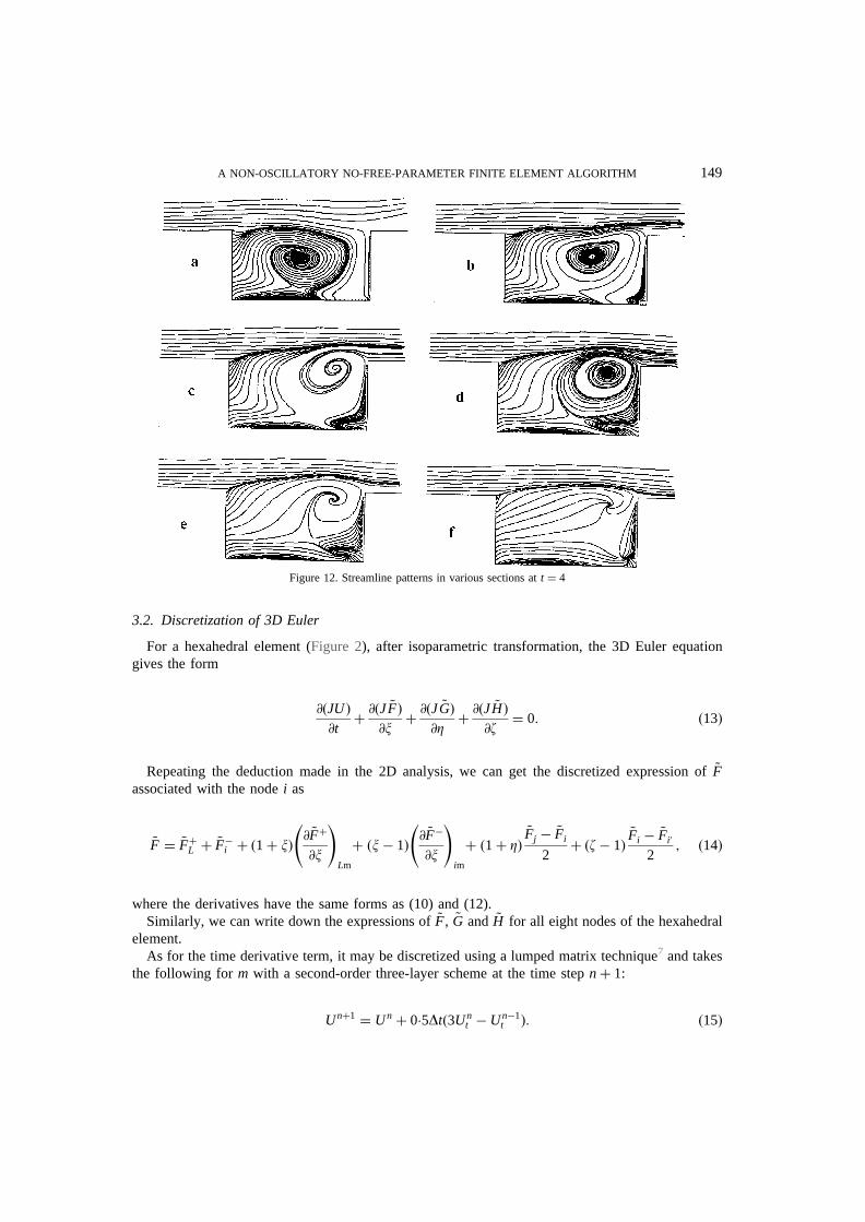
Figure 12. Streamline patterns in various sections att � 4


4. APPLICATIONS OF NNFEM IN CFD

The present algorithm has been successfully checked in various cases: regular reflection of an obliqueshock wave on a flat plate, supersonic flow over a forward step and axisymmetric free jet flow with avery high pressure ratio. It has also been applied with great success to the numerical study ofsupersonic flows over 2D and 3D rectangular cavities.

4.1. Inviscid oblique shock wave reflection

The first case computed is the regular reflection of an inviscid oblique shock wave (f � 29�) on aflat plate withM

1

� 2�9 and a uniform isotropic grid of 1216 31 points.Figures 3(a)and 3(b) showrespectively the pressure contours and the pressure distribution along a grid line ony � 0�5. Nospurious oscillations were found in the shock wave region and the computational resolution for theshock wave is obviously better than that given by a first-order upwind scheme (Figure 3(c)).

4.2. Supersonic flow over a forward step

Based on the 2D N–S equations, the supersonic flow ofM1

� 2�3 over a forward step with thelength–height ratioL=H � 27�7 andRe

1;H � 7200 has been computed with the node number 16,400,where refinement of the grids is made just near the viscous wall. As shown inFigure 4, the graph ofdensity contours results in good resolution in the whole flow field. The pressure distribution along thewall compares well with the experimental data of Reference 8, as seen inFigure 5.

Based on the Euler equations, the axisymmetric free jet flow in still air�M1

� 0� with the exitconditionMj � 1, the ratio of the surrounding pressure to the total exit pressurep

1

=poj � 1=50 andthe temperature ratioT

1

=Toj � 1 has been computed with the node number 61661. It is well knownthat this was a difficult case for finite element simulation in the past because of the very strong shock

Figure 13. Streamline patterns in various sectrions att � 5

150 Y. WANG ET AL.

wave (Mach disc) involved. The density and pressure contours are shown inFigures 6(a)and 6(b)respectively, where we can clearly see a Mach disc located at a distance of about five exit diametersand the interaction between the Mach disc and a drum-like shock wave, which gives evidence of goodcomputational resolution and no spurious oscillations across these shocks.Figure 7shows the Machnumber distribution along the centreline, which is in excellent agreement with the finite differencecomputational result of Reference 2.

4.3. Supersonic flow over a 2D rectangular cavity

Based on the N–S equations, the supersonic flow ofM1

� 1�5 over a 2D rectangular cavity withthe length–height ratioL=H � 2 andRe

1;L � 105 has been predicted with the node number 61631in the cavity. The density contours of this flow at various times are shown inFigure 8, where we canclearly see the shock wave translating in a periodic motion and also the periodic vortex motion.Figure 9shows the corresponding distributions along the bottom of the cavity. These phenomena areconsistent with the experimental observations of Reference 9.

The supersonic flow of M1

� 1�5 over a 3D rectangular cavity (Figure 10) withL : H : W � 2 : 1 : 1 and Re

1;L � 105 has been computed with the node number 316316 15 inthe cavity. The density contours in the symmetric section of the cavity at various times are shown inFigure 11, where periodic motions of the shock wave and vortex flow, similar to the 2D case, can bedetected.Figures 12–15shown the streamline patterns of the cavity flow in its various sections atfour time steps. We are not ready to discuss the flow physics in this paper, other than to note that it isa very complex unsteady separated and vortical flow with very interesting topological structures,including temporal changes in nodal points and saddle points and a transformation between separatedand attached spiral points through limit cycles.

Figure 14. Streamline patterns in various sections att � 5�5


5. CONCLUSIONS

A non-oscillatory no-free-parameter finite element algorithm has been constructed on a physicalbasis, considering wave propagation characteristics in different characteristic directions across astrong discontinuity through flux splitting and Taylor series expansion in order to get a reasonabledistribution of inviscid fluxes in every element and satisfy the increasing entropy condition. Itsapplications to steady and unsteady complex flows of shock wave interactions and massive separationwith vortex motions have identified that the present algorithm gives good computational resolutionwithout spurious oscillations in the shock wave region as well as in the whole flow field. Also, it isstable in operation and efficient in practice.

ACKNOWLEDGEMENTS

This study is supported by the National Natural Science Foundation of China. The authors aregrateful to Dr. Bo-Nan Jiang for his valuable suggestions.

REFERENCES

1. A. Harten, ‘On a class of high resolution total variation-stable finite difference schemes’,SIAM J. Anal., 21, 1–23 (1984).2. H. X. Zhang and F. G. Zhuang, ‘NND schemes and their applications to numerical simulation of two and three dimensional

flows’, Adv. Appl. Mech., 29, 193–256 (1992).3. T. J. R. Hughes and Mallet, ‘Recent progress in the development and understanding of SUPG methods with special

reference to the compressible Euler and Navier–Stokes equations’,Int. j. numer. methods fluids, 7, 1261–1275 (1987).4. A. J. Baker and J. W. Kim, ‘Statement of algorithm for hypersonic conservation laws’,Int. j. numer methods fluids, 7, 498–

520 (1987).

Figure 15. Streamline patterns in various sections att � 6�3

152 Y. WANG ET AL.

5. R. Ramakrishman, K. S. Bey and E. A. Thorton, ‘An adaptive quadrilateral and triangular finite element scheme forcompressible flows’,AIAA Paper 88-0033, 1988.

6. J. L. Steger and R. F. Warming, ‘Flux vector splitting of the inviscid gasdynamic equations with applications to finitedifference methods’,J. Comput. Phys., 40, 263–293 (1981).

7. K. S. Bey and E. A. Thorton, ‘A new finite element approach for prediction of aerothermal and loads–progress in inviscidflow computations’,NASA-TM-86434, 1985.

8. D. R. Chapman, D. M. Kuehn and H. K. Larson, ‘Investigation of separated flows in supersonic and subsonic streams withemphasis on the effect of transition’,NACA Rep. 1356, 1958.

9. H. H. Heler and D. B. Bliss, ‘Aerodynamically induced pressure oscillations in cavities-physical mechanisms andsuppression concepts’,AFFDL-TR-74-13, 1974.


a non-oscillatory no-free-parameter finite element and its applications in cdf

Documents