a new wind turbine control method to smooth power...
TRANSCRIPT
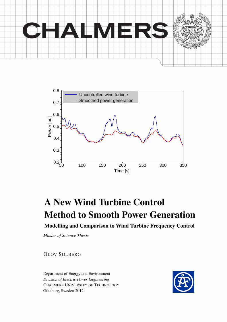
Uncontrolled wind turbineSmoothed power generation
0.2
0.3
0.4
0.5
0.6
0.7
0.8
50 100 150 200 250 300 350Time [s]
Pow
er [p
u]
A New Wind Turbine ControlMethod to Smooth Power GenerationModelling and Comparison to Wind Turbine Frequency Control
Master of Science Thesis
OLOV SOLBERG
Department of Energy and EnvironmentDivision of Electric Power EngineeringCHALMERS UNIVERSITY OF TECHNOLOGY
Goteborg, Sweden 2012


A New Wind Turbine Control Methodto Smooth Power Generation
Modelling and Comparison to Wind Turbine Frequency Control
OLOV SOLBERG
Department of Energy and EnvironmentDivision of Electric Power Engineering
CHALMERS UNIVERSITY OF TECHNOLOGYGoteborg, Sweden 2012

A New Wind Turbine Control Method to Smooth Power GenerationModelling and Comparison to Wind Turbine Frequency ControlOLOV SOLBERG
c© OLOV SOLBERG, 2012.
Department of Energy and EnvironmentDivision of Electric Power EngineeringCHALMERS UNIVERSITY OF TECHNOLOGY
SE–412 96 GoteborgSwedenTelephone +46 (0)31–772 1000
Cover:Smoothed wind power production using a pitch angle offset of 3.3◦ under normal windconditions.
Chalmers Bibliotek, ReproserviceGoteborg, Sweden 2012

A New Wind Turbine Control Method to Smooth Power GenerationModelling and Comparison to Wind Turbine Frequency ControlOLOV SOLBERGDepartment of Energy and EnvironmentDivision of Electric Power EngineeringChalmers University of Technology
Abstract
Following the significant increase of world wide installed wind power during the first decade ofthe 21st century, transmission system operators are faced with new challenges originating fromthe intermittent character of renewable energy sources and their installation on low and mediumvoltage levels. One challenge arising from the fluctuating nature of wind is to maintain frequencystability. This thesis presents a new approach to smooth the power generation of wind turbinessubjected to varying wind. An active power feedback control has been developed which feedsback the momentary power generation to the turbine pitch and speed control systems. This powerfeedback control has been implemented in the simulation software SIMPOW and the results havebeen compared to a frequency control regulator for wind turbines. The frequency control wasdeveloped by the Power System Analysis Group at AF Industry as a part of the Swedish researchinitiative Elforsk.
Simulation results show that the power feedback control clearly levels the active power produc-tion of wind turbines under varying wind and thereby diminishes network frequency excursions.To achieve this, turbine deloading through a pitch angle offset is found to be imperative. Theeffect of different deloading levels of a turbine are evaluated, clearly demonstrating the correlationbetween larger deloading, enhanced frequency stability and declining energy yield. Up to windpower shares of approximately 25 %, the performance of the power feedback control is on a parwith the frequency control, i.e., frequency excursions are equally subdued. Above this level ofinstalled wind power, the frequency control is superior. Usage of the wind turbine power feedbackcontrol is discouraged because of its poorer performance, its unintuitive function and the difficultyto predict its behaviour. Lastly, the frequency control is applied to a much simplified black startcase, showing the expediency of the control method to improve frequency stability, but also theextended requirement on a large turbine deloading when there are no synchronously generatingunits in the network.
Index Terms: Wind power, active power feedback control, frequency control, power smoothing,wind turbine deloading, fluctuating wind, black start.
iii

iv

Acknowledgements
This thesis was carried out at AF Industry, Goteborg, as a graduation from Chalmers University ofTechnology.
I would like to thank my examiner Peiyuan Chen at Chalmers, my supervisor Robert Josefssonat AF, and Mats Wang-Hansen and Haris Mehmedovic at AF. Thank you for your guidance andpatience with my many questions, without which this work would not have been completed.
My special gratitude goes to my wife Elin. Thank you dear for always loving and supporting me.
All glory to the only wise God, through Jesus Christ, forever.
Olov SolbergGoteborg, Sweden, 2012
v

vi

Contents
Abstract iii
Acknowledgements v
1 Introduction 11.1 Background . . . . . . . . . . . . . . . . . . . . . . . . . . . . . . . . . . . . . 11.2 Purpose . . . . . . . . . . . . . . . . . . . . . . . . . . . . . . . . . . . . . . . 11.3 Area of Investigation . . . . . . . . . . . . . . . . . . . . . . . . . . . . . . . . 21.4 Outline of Report . . . . . . . . . . . . . . . . . . . . . . . . . . . . . . . . . . 2
2 Frequency Control of Power Systems with Wind Power 32.1 Power System Frequency Control Principles . . . . . . . . . . . . . . . . . . . . 3
2.1.1 Generation Characteristics . . . . . . . . . . . . . . . . . . . . . . . . . 42.1.2 Primary Control . . . . . . . . . . . . . . . . . . . . . . . . . . . . . . 52.1.3 Secondary Control . . . . . . . . . . . . . . . . . . . . . . . . . . . . . 6
2.2 Wind Turbines and Generator Systems . . . . . . . . . . . . . . . . . . . . . . . 72.2.1 Fixed-Speed Wind Turbines . . . . . . . . . . . . . . . . . . . . . . . . 82.2.2 Variable-Speed Wind Turbines . . . . . . . . . . . . . . . . . . . . . . . 8
2.3 Operation of Wind Turbines . . . . . . . . . . . . . . . . . . . . . . . . . . . . 102.3.1 Deloading Strategies . . . . . . . . . . . . . . . . . . . . . . . . . . . . 102.3.2 Deloading Implementation . . . . . . . . . . . . . . . . . . . . . . . . . 10
3 Default Wind Power Modelling in SIMPOW 133.1 Power Flow Calculation and Dynamic Simulation . . . . . . . . . . . . . . . . . 133.2 Wind Turbine Modelling . . . . . . . . . . . . . . . . . . . . . . . . . . . . . . 143.3 Wind Farm Modelling . . . . . . . . . . . . . . . . . . . . . . . . . . . . . . . . 153.4 Synchronous Generator . . . . . . . . . . . . . . . . . . . . . . . . . . . . . . . 153.5 Power Electronic Converter . . . . . . . . . . . . . . . . . . . . . . . . . . . . . 153.6 Speed Control . . . . . . . . . . . . . . . . . . . . . . . . . . . . . . . . . . . . 16
3.6.1 Default Calculation of the Speed Reference . . . . . . . . . . . . . . . . 173.7 Pitch Control . . . . . . . . . . . . . . . . . . . . . . . . . . . . . . . . . . . . 193.8 AC Voltage Control . . . . . . . . . . . . . . . . . . . . . . . . . . . . . . . . . 203.9 Wind Data . . . . . . . . . . . . . . . . . . . . . . . . . . . . . . . . . . . . . . 20
4 Wind Turbine Regulators for Frequency and Power Smoothing Control 214.1 Frequency Regulator (f-reg) . . . . . . . . . . . . . . . . . . . . . . . . . . . . 214.2 Active Power Feedback Regulator (P-reg) . . . . . . . . . . . . . . . . . . . . . 21
4.2.1 Calculation of the Power Set Point . . . . . . . . . . . . . . . . . . . . . 224.3 Combined Frequency and Active Power Feedback Regulator (c-reg) . . . . . . . 24
vii

CONTENTS
5 Adapted Modelling of the Wind Power Speed Controller 275.1 Modified Calculation of the Speed Reference . . . . . . . . . . . . . . . . . . . 275.2 Demonstration of the Modified Speed Controller . . . . . . . . . . . . . . . . . 28
6 Results and Analysis of Frequency and Active Power Feedback Control 316.1 Simulated Power System . . . . . . . . . . . . . . . . . . . . . . . . . . . . . . 316.2 Wind Power Data . . . . . . . . . . . . . . . . . . . . . . . . . . . . . . . . . . 326.3 Comparison of Deloading Levels . . . . . . . . . . . . . . . . . . . . . . . . . . 33
6.3.1 Maximum Power Point Tracking . . . . . . . . . . . . . . . . . . . . . . 346.3.2 Frequency Control . . . . . . . . . . . . . . . . . . . . . . . . . . . . . 366.3.3 Active Power Feedback Control . . . . . . . . . . . . . . . . . . . . . . 376.3.4 Concluding Remark - Comparison of Deloading Levels . . . . . . . . . . 37
6.4 Comparison of Frequency Control and Active Power Feedback Control . . . . . 386.4.1 Normal Wind Variations . . . . . . . . . . . . . . . . . . . . . . . . . . 386.4.2 Extreme Wind Variations . . . . . . . . . . . . . . . . . . . . . . . . . . 406.4.3 Concluding Remark - Comparison of Frequency Control and Active Power
Feedback Control . . . . . . . . . . . . . . . . . . . . . . . . . . . . . . 416.5 Comparison of Frequency Control and Active Power Feedback Control with In-
creased Wind Power Share . . . . . . . . . . . . . . . . . . . . . . . . . . . . . 426.6 Comparison of Active Power Feedback Regulation with and without Regulated
Pitch Control . . . . . . . . . . . . . . . . . . . . . . . . . . . . . . . . . . . . 436.6.1 0◦ Deloading . . . . . . . . . . . . . . . . . . . . . . . . . . . . . . . . 436.6.2 3.3◦ Deloading . . . . . . . . . . . . . . . . . . . . . . . . . . . . . . . 456.6.3 Concluding Remark - Comparison of Active Power Feedback Regulation
with and without Regulated Pitch Control . . . . . . . . . . . . . . . . . 45
7 Application of Full Power Converter Wind Turbines to Power System Black Start 477.1 Description of the Simulated Case . . . . . . . . . . . . . . . . . . . . . . . . . 487.2 Induction Machine Load . . . . . . . . . . . . . . . . . . . . . . . . . . . . . . 48
7.2.1 Without Frequency Control . . . . . . . . . . . . . . . . . . . . . . . . 487.2.2 With Frequency Control . . . . . . . . . . . . . . . . . . . . . . . . . . 517.2.3 Fluctuating Wind Conditions . . . . . . . . . . . . . . . . . . . . . . . . 517.2.4 Concluding Remark - Induction Machine Load . . . . . . . . . . . . . . 52
8 Conclusions 538.1 Outlook . . . . . . . . . . . . . . . . . . . . . . . . . . . . . . . . . . . . . . . 54
References 55
viii

List of Figures
2.1 Steady state speed-droop characteristic for a turbine-governor . . . . . . . . . . . 42.2 System generation characteristic. . . . . . . . . . . . . . . . . . . . . . . . . . . 52.3 Schematic of the action of the primary and secondary frequency control. . . . . . 62.4 Typical form of a cp(λ) curve. . . . . . . . . . . . . . . . . . . . . . . . . . . . 72.5 A fixed-speed wind turbine with a squirrel-cage induction generator. . . . . . . . 82.6 A variable-speed wind turbine with a doubly-fed induction generator (DFIG). . . 92.7 A variable-speed wind turbine with a wound rotor synchronous generator inter-
faced via a fully rated power electronic converter. . . . . . . . . . . . . . . . . . 102.8 Illustration of different deloading options. . . . . . . . . . . . . . . . . . . . . . 112.9 Wind turbine power as a function of the turbine speed. Under and over speeding
in comparison to MPPT operation. . . . . . . . . . . . . . . . . . . . . . . . . . 11
3.1 Block diagram of the SIMPOW FPCWT model and main communication betweenits modules. . . . . . . . . . . . . . . . . . . . . . . . . . . . . . . . . . . . . . 14
3.2 PWM converter model in SIMPOW. . . . . . . . . . . . . . . . . . . . . . . . . 153.3 Schematic of the unregulated wind turbine speed controller system. . . . . . . . 163.4 Overall wind turbine operation as governed by the speed and pitch controllers. . . 173.5 Speed reference curve for a wind turbine with a rated wind speed of 12 m/s, using
the default speed controller in SIMPOW. . . . . . . . . . . . . . . . . . . . . . . 193.6 Schematic of the unregulated wind turbine pitch controller system. . . . . . . . . 193.7 AC voltage control of PWM converters in SIMPOW. . . . . . . . . . . . . . . . 20
4.1 Schematic of the wind turbine speed controller featuring frequency control. . . . 224.2 Schematic of the wind turbine pitch controller featuring frequency control. . . . . 224.3 Simplified block diagram of the wind turbine speed controller featuring active
power feedback control. . . . . . . . . . . . . . . . . . . . . . . . . . . . . . . . 234.4 Simplified block diagram of the wind turbine pitch controller featuring active
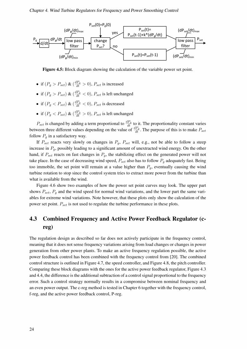
power feedback control. . . . . . . . . . . . . . . . . . . . . . . . . . . . . . . . 234.5 Block diagram showing the calculation of the variable power set point. . . . . . . 244.6 Power set point Pset plotted together with the wind speed and the produced power
Pg of the unregulated wind turbine. . . . . . . . . . . . . . . . . . . . . . . . . . 254.7 Simplified block diagram of the wind turbine speed controller featuring frequency
control and active power feedback control. . . . . . . . . . . . . . . . . . . . . . 264.8 Simplified block diagram of the wind turbine pitch controller featuring frequency
control and active power feedback control. . . . . . . . . . . . . . . . . . . . . . 26
5.1 Speed reference curve for a wind turbine with a rated wind speed of 12 m/s, usingthe modified speed controller. . . . . . . . . . . . . . . . . . . . . . . . . . . . . 28
5.2 Demonstration of the wind turbine model using the modified speed controller. . . 29
ix

LIST OF FIGURES
6.1 Topology of the simulated power system. . . . . . . . . . . . . . . . . . . . . . 326.2 cp(λ) curves used in the simulations. . . . . . . . . . . . . . . . . . . . . . . . . 336.3 Frequency for different deloading levels running MPPT mode, normal wind. . . . 356.4 Generated power for different deloading levels running MPPT mode, normal wind. 356.5 Frequency for different deloading levels running f-reg mode, normal wind. . . . . 366.6 Frequency for different deloading levels running P-reg mode, normal wind. . . . 376.7 Frequency for different regulation methods with β0 = 3.3◦, normal wind. . . . . 386.8 Power for different regulation methods with β0 = 3.3◦, normal wind. . . . . . . . 396.9 Pitch angle for different regulation methods with β0 = 3.3◦, normal wind. . . . . 396.10 Frequency for different regulation methods with β0 = 3.3◦, extreme wind. . . . . 406.11 Frequency for different regulation methods when increasing the wind power pen-
etration, β0 = 3.3◦ and normal wind. . . . . . . . . . . . . . . . . . . . . . . . . 426.12 Frequency, with and without regulated pitch controller, β0 = 0◦ and normal wind. 436.13 Power, with and without regulated pitch controller, β0 = 0◦ and normal wind. . . 446.14 Pitch angle, with and without regulated pitch controller, β0 = 0◦ and normal wind. 446.15 Frequency, with and without regulated pitch controller, β0 = 3.3◦ and normal wind. 45
7.1 System layout of the small power system used for simplified black start studies. . 487.2 Standard torque speed curve of an induction machine. . . . . . . . . . . . . . . . 497.3 Grid frequency, wind turbine power and pitch angle using an unregulated wind
turbine and an induction machine load. . . . . . . . . . . . . . . . . . . . . . . . 497.4 Induction machine power, speed and torque, and grid voltage, using an unregulated
wind turbine. . . . . . . . . . . . . . . . . . . . . . . . . . . . . . . . . . . . . 507.5 Active and reactive power generation of the synchronous generator and the wind
turbine, using the an unregulated wind turbine and an induction machine load. . . 507.6 Grid frequency, wind turbine power and pitch angle using an induction machine
load and applying frequency control to the wind turbine. . . . . . . . . . . . . . 517.7 Grid frequency, wind turbine power and pitch angle using an induction machine
load and applying frequency control to the wind turbine under normal wind fluc-tuations. . . . . . . . . . . . . . . . . . . . . . . . . . . . . . . . . . . . . . . . 52
x

Chapter 1
Introduction
The main objective for this master thesis project is to implement a wind turbine regulator in orderto control the generation of active power. This regulator should use the active power generationas a feedback signal. The aim is to smooth wind induced frequency variations by smoothing theactive power generation. To evaluate the effectiveness of the power control, a comparison to windturbine frequency control is made. Additionally, the possibility of applying frequency control towind turbines in black start scenarios is briefly introduced.
1.1 Background
Traditionally, electric power has been generated by large power stations such as nuclear, hydroor thermal power plants. During the entire 20th century, wind power constituted an insignificantpart of the total power production, making it easy for grid utilities to integrate with conventionalgenerating facilities. From year 2001 to 2010, the amount of installed wind power worldwide hasmultiplied more than eight times [22]. This development has not left the electric grid industryunaffected and system operators are challenged with new stability issues. To aid in the frequencycontrol of a power system, it is therefore advantageous if wind farms can contribute to frequencyregulation. In fact, according to the draft of the upcoming harmonized European grid codes [8],all kinds of power plants will be required to assist in frequency control. However, wind power notonly causes new challenges. One advantage arising with more installed wind power is the prospectof using wind turbines to black start a grid or to supply grid islands. Such a development couldhelp reduce the number of backup diesel generators, as well as increasing power system reliability.
1.2 Purpose
The present thesis is in many ways a direct continuation of the reports [20] and [21]. These projectshave been carried out by the Power System Analysis Group at AF Industry in Gothenburg, Sweden.The later report from AF, [20], presents a way to regulate the power of a wind turbine using thegrid frequency deviation as an input signal. Drawing on the simulation models of that work, thepurpose of this thesis project is to develop and evaluate a method to level the wind turbine powergeneration when using the momentary active power production as a feedback signal instead of thefrequency deviation. A smooth power output will, as long as the load is constant, contribute to asmoother frequency during wind fluctuations.
One of the main goals is the comparison with the work done by AF, to investigate if this alter-native control approach may be a viable choice. There are also many other scientific publications
1

Chapter 1. Introduction
dealing with the issue of frequency control support from wind power plants. Some of these articlesare presented and referenced in Section 2.3, Operation of Wind Turbines.
1.3 Area of Investigation
Using the power system simulation software SIMPOW [17], the result of the above describedactive power control strategy is studied. First and foremost, the wind turbine active power output,rotational speed, pitch angle and grid frequency are compared. The special interest of this thesislies in the implementation and evaluation of the power control method when using the active poweras a feedback signal to the turbine speed and pitch controllers. Further, this work incorporatesexperimental wind data which subjects the simulated wind turbine to fluctuating, i.e., realistic,wind conditions.
1.4 Outline of Report
Following the introduction in Chapter 1, Chapter 2 first presents an overview of the theory ofpower system frequency control. After that, different wind turbine systems are explained as wellas different operational strategies and ways to deload a wind turbine. The 3rd chapter is dedicatedto a description of the default wind turbine model used in SIMPOW. Chapter 4 details the differentcontrol strategies used in this work and Chapter 5 describes the improvements done to the defaultSIMPOW wind power model. The simulation set up and results are presented and analysed inChapter 6. As an extension to the initial frequency control problem, an application of wind turbinesto power system black start is thereafter presented in Chapter 7. Finally, conclusions are presentedin Chapter 8 together with an outlook of future work.
2

Chapter 2
Frequency Control of Power Systemswith Wind Power
In electric power systems, many power plants cooperate to make sure that the electric load is sup-plied. Synchronous generators form the bulk of this generation capacity, especially in steam andhydro power plants. To secure a safe power system operation, there has to be control systems foractive and reactive power, influencing mainly the grid frequency and voltage. Apart from conven-tional generation, modern power systems include a larger share of renewable generation such aswind and solar power. To make these integrate well with the rest of the power system, differentoperational strategies are continuously being developed, especially for wind turbines. There arealso different wind turbine-generator configurations, providing different control possibilities. Thefollowing chapter provides a condensed theoretical overview of these topics, which have beendeemed relevant to this report.
2.1 Power System Frequency Control Principles
Maintaining the power system frequency is a matter of maintaining the balance between powerproduction and consumption. Since the use of large scale power storage systems is very limitedtoday, the electric power production has to match the electric power consumption at any givenmoment. If it does, there is an active power balance in the system and the frequency will remainconstant. If it does not, the frequency will change. In large interconnected systems, frequency vari-ations seldom exceed ±0.1 Hz [7], whereas in autonomous island systems, frequency variationsup to ±1 Hz are not uncommon [4].
In today’s power system, mainly synchronous generators are used to produce electric power.These generators induce voltages with the same frequency as the rotational speed of the unit, ex-cept for the scaling of the number of pole pairs. This means that when the grid frequency changes,it does so because the speed of the synchronous generators are changing. Looking at each genera-tor, to maintain steady state there has to be a balance between the driving mechanical torque Tmand the braking electrical torque Te. This relation can be expressed as
Tm − Te = Jdω
dt(2.1)
where J is the moment of inertia of the system and ω is the generator speed. The moment ofinertia is the sum of the turbine, shaft and rotor inertia. Since torque is equal to power divided byangular frequency, dω
dt will equal zero if the mechanically supplied power Pm equals the electri-cally generated power Pe, neglecting generator losses. From (2.1) it can also be seen that if thereis is a torque imbalance, the generator will change its rotational speed. If, e.g., the load increases,
3

Chapter 2. Frequency Control of Power Systems with Wind Power
meaning that Te increases, while the driving torque remains constant, then dωdt will be negative and
the generator will decelerate. In this way, kinetic energy is converted to electrical energy to supplythe load increase [7], [10].
2.1.1 Generation Characteristics
As described in the previous section, a stable operation of a turbine must have a power-speedcharacteristic such that the mechanical power increases when the speed decreases, and inverselythe mechanical power has to decrease when the speed increases. To regulate the power and speed,turbine governors are used to achieve the desired characteristic. A typical turbine governor controlcan be expressed as
∆Pm = − 1
R∆ω (2.2)
in steady state. The power difference ∆Pm is the change in turbine mechanical power output,∆ω is the change in speed and R is known as the regulation constant [10]. The inverse of R,namely 1
R , is known as the speed-droop coefficient or simply as the droop [14]. Since the speed ofsynchronous generators is proportional to the grid frequency, (2.2) can be rewritten as
∆Pm = − 1
R∆f, (2.3)
using per-unit quantities in (2.2) and (2.3). Figure 2.1 shows a standard steady state speed-droopcharacteristic of a turbine with slope −R. This is also the steady state frequency power relation.In this figure, the turbine is operational within the interval of Pmin to Pmax, being limited at thebottom by technical parameters such as burner stability in coal plants and at the top by thermaland mechanical considerations [14]. At Pmax, the turbine power production does not increase anylonger with decreased frequency.
f
fn
PmPmaxPmin Pn
Figure 2.1: Steady state speed-droop characteristic for a turbine-governor
In a real power system, many generating units are operating synchronously at the same fre-quency. To obtain the complete generation characteristic of the whole system, the speed-droopcharacteristics of all individual turbines are added. During normal operation of a power system,many turbines will not be loaded to their maximum level. This means that there is a reserve gen-erating capacity from generators that are online, but operating at partial loading. This reserve iscalled the spinning reserve, which is defined as the difference between the sum of the turbine powerratings and total system load. Due to different loading levels of the turbines and the spinning re-serve, the complete system generation characteristic will be a non-linear curve as the one shown inFigure 2.2. For practical reasons, this curve may be linearized in the vicinity of the operating pointwhen analysing small frequency and power fluctuations. It can be noted that the droop, the slope ofthe generation characteristic, becomes infinite at Pmax, as is shown by the dashed line. This wouldbe the theoretical case when all generators are operating at their maximum power output level and
4

2.1. Power System Frequency Control Principles
the spinning reserve is down to zero. In reality, however, power plants usually have a frequencydependent so-called curled-back characteristic, which makes the total speed-droop curve have thisfeature as well [14].
f
PmPmax
Figure 2.2: System generation characteristic.
2.1.2 Primary Control
The main goal of primary control is to stop the change in frequency and make the power systemreach a new steady state frequency. When a power system event occurs which affects the frequency,e.g. the loss of a generator or a load step, the very first thing to happen is that the rotational speedof the turbine-generator is affected by a transient extraction or addition of kinetic energy. Whenthe frequency changes, the primary control comes into action. First, the speed deviation is sensedby the speed-governing system. The speed deviation signal will be passed through a PI regulatorand sent as a control signal to actuate the valves or gates of the turbine [12]. This will increaseor decrease the turbine action, depending on whether the frequency has dropped or raised. Theintegral action will make the system reach a new steady state, though at an off-nominal frequencydue to the droop characteristic according to Figure 2.1.
Normally, the aggregated load of a power system will change according to the frequency,i.e., it is not a constant power load. The frequency sensitivity of the load is opposite to that ofthe turbine-governor characteristic, so that when the frequency decreases, the load demand willdecrease and vice versa. Most commonly, the generation frequency dependency is much largerthan the load frequency sensitivity, meaning that the change in power generation is much largerthan the change in load demand when subjected to equal frequency deviations [14]. As indicated inFigure 2.2, an increase in total system power is only possible when there is a spinning reserve, i.e.,when there are generating units operating at partial load. These partially loaded generators shouldideally be spread out to all areas of a power system in order not to overload transmission lineswhen an area of the power system requires extra power from a spinning reserve located far away.In an interconnected system, according to the solidarity principle, each control area is thereforeexpected to provide a spinning reserve proportional to its share in the whole synchronised area.
Production units participating in primary control are controlled with a dead band for theirfrequency set points. Different grid codes put different requirements on how fast part of, and thewhole, spinning reserve should be activated. Generally, the part of the spinning reserve whichis available for primary frequency control should be fully accessible within 15-23 seconds [14].In the Nordic grid code [16], it is stipulated that the primary reserve should always be activatedwhen the frequency reaches 49.9 Hz. In the event of a frequency drop to 49.5 Hz, 50% of theprimary reserve power is obliged to be regulated upwards within 5 seconds, and 100% within 30seconds. If, e.g., a significant production unit is unexpectedly lost, there will be a rapid reductionin frequency. Initially, rotor swings in generators will occur since kinetic energy is extracted from
5

Chapter 2. Frequency Control of Power Systems with Wind Power
all synchronously operating turbine-generators. The power support achieved in this way will bebrief and likely insufficient, depending on the size of the outage. When the grid frequency drops,the primary control is activated and the spinning reserve power should be fully online in less thanhalf a minute, as can be seen in Figure 2.3.
Figure 2.3: Schematic of the action of the primary and secondary frequency control. The upperFigure shows a possible frequency response in case of a generation outage. The lower Figureshows the working of the primary control power (red curve) and the secondary control power(blue curve). Figure adopted from [11].
2.1.3 Secondary Control
Follwing the action of a successful primary frequency control, the grid frequency will be stable atan off-nominal frequency. The main task of the secondary control is to take care of this frequencydeviation and bring back the steady state frequency to its nominal value, as shown in Figure 2.3.At the same time, it can be seen that the secondary control restores the primary frequency controlreserve. Finally, the secondary control is also responsible for guaranteeing that scheduled tie linepower interchanges are maintained. This is important since is assures that each control area of aninterconnected power system absorbs its own load changes, which is called the non-interventionrule. In such systems, secondary control is always decentralized since the regulator control loopsare not able to sense where a power deficit occurs. Using centralized secondary control wouldtherefore result in unwanted tie-line power flows, violating inter-operator agreements [14]. Sec-ondary control is performed through altered power reference levels of turbine governors. This willresult in the frequency-power curve of Figure 2.1 being moved up (dash-dotted line). Thereby, thepower production will be able to meet the load level at nominal frequency, which is the desiredgoal of the load-frequency control. In the Nordic power system, automatic secondary control isnot used. The means to regain nominal frequency is instead to manually adjust the power refer-ence levels of production units, a procedure which is sometimes referred to as tertiary control. Inthe UCTE grid of the European continent, secondary control is handled automatically, so-calledautomatic generation control.
6

2.2. Wind Turbines and Generator Systems
2.2 Wind Turbines and Generator Systems
Wind power plants use wind turbines to extract the power contained in the wind. The amount ofpower that can be extracted from the wind is equal to the power which is physically contained inthe moving mass of the air, multiplied by the factor cp. This is expressed as
Pwind =1
2cpρAv
3wind, (2.4)
where ρ is the air density, A the area swept by the turbine and vwind the wind speed. The constantcp has a maximum theoretical value of 0.599, which is termed Betz limit after the discovery byBetz in 1926 [1], [14]. As can be seen in (2.4), wind power is proportional to the cube of the windspeed. This means that even small wind fluctuations will impact the generated power significantly.Another important quantity is the tip speed ratio λ, which is defined as
λ =vtipvwind
=Rω
vwind. (2.5)
In this case, the blade tip speed vtip and the wind speed vwind are given in m/s, R is the turbineradius in m, i.e., the blade length, and ω is the turbine rotation in radians per second. Once againlooking at (2.4), it is obvious that a high wind speed, a large turbine swept area and a high value ofcp will all lead to a high power being generated by the wind power plant. Among these parameters,cp, which depends on λ, is the only one that can be controlled. Therefore, adjusting λ so that cpreaches its maximum value is a natural strategy when operating a wind turbine. To do this, vtiphas to be adjusted and therefore this operational method called Maximum Power Point Tracking(MPPT) is primarily used by variable-speed wind turbines. Figure 2.4 shows the typical form ofa cp(λ) curve, whose exact form differs between different wind turbines and is often determinedthrough experimental set-ups.
λ
cp
Figure 2.4: Typical form of a cp(λ) curve.
In addition to turbine speed control, the aerodynamic force of a wind turbine is controlled tohelp regulate the power production. This is especially applied to protect the wind turbine fromtoo high wind speeds. During stormy weather conditions, wind turbines have to shut down andlock their blades in order not to be damaged due to too high mechanical stress. The aerodynamiccontrol can be done in three different ways: stall control, pitch control and active stall control. Stallcontrol is the simplest and most robust way of controlling the aerodynamic forces. In this case, theblades are mounted to the hub with a fixed angle towards the wind. The blades are designed in sucha way that when the wind speed increases, the wind absorbing ability of the blades decrease andthe rotor will stall above a given wind speed. In contrast to the passive stall control, pitch controloffers an active way of controlling the aerodynamic force absorption. In such a configuration, theblades can be turned out of or into the wind, i.e., they can be pitched. This will change the angle ofthe blades, affecting how well they absorb wind. At wind speeds exceeding the construction limit
7

Chapter 2. Frequency Control of Power Systems with Wind Power
of the turbine, the blades pitch completely, minimizing the aerodynamic performance of the rotorand making it stop rotating. The third option of aerodynamic control is the active stall control.As the name indicates, the stall of the blades is actively controlled through pitching. At low windspeeds, the blades are pitched to achieve maximum efficiency and at excessive wind speeds, theblades are slightly pitched in the opposite direction of standard pitch control, making the bladesstall further. Of these power control concepts, all three are used in combination with fixed-speedturbines whereas only pitch control is used with variable-speed turbines [1].
2.2.1 Fixed-Speed Wind Turbines
In spite of the benefits of adapting the turbine rotation and thereby controlling the tip speed ratio λ,fixed-speed wind turbines are the traditionally favoured wind power concept. An example of sucha turbine-generator configuration is shown in Figure 2.5. A fixed-speed turbine operates at a nearlyconstant speed determined by the grid frequency and the gearbox ratio. The turbine is connectedto an induction generator which can be of two types, with a squirrel-cage (short circuited) rotoror with a wound rotor. Of these two, the squirrel-cage rotor is the simplest construction, but thespeed variability is limited to that of the slip of the induction machine. Using a wound rotor, therotor resistance can be controlled, allowing a somewhat higher speed operating range. In eithercase, the connection between the turbine and the grid is rather stiff, which means that the transienttorques caused by wind gusts will cause considerable gearbox wear. Furthermore, the stator ofthe induction machine may be equipped with two different sets of windings, one with eight polesused to operate at low wind speeds and one with four to six poles used during higher wind speedconditions. Apart from the limited speed elasticity, the main disadvantage of fixed-speed turbinesusing induction machines is their need for a magnetising current. This reactive current has to bedrawn from the grid if it is not supplied by e.g. shunt capacitors. Still, fixed-speed turbines havebeen widely used due to their overall robust and simple construction and their cheap electricalcomponents [1], [14].
1:n IG
Figure 2.5: A fixed-speed wind turbine with a squirrel-cage induction generator.
2.2.2 Variable-Speed Wind Turbines
During the last decade, variable-speed wind turbines have gained favour and among newly in-stalled turbines, they are almost exclusively chosen. The main reason for this is their better energycapture and thereby their better economic yield. To permit a varying speed, power electronic con-verters are added to the generator configuration. In this way, wind gusts are absorbed primarilyby changes in the generator speed and in contrast to fixed-speed turbines, the generator torque iskept fairly constant. In addition to increased energy yield, the use of power electronics enablesthe wind turbine to control active and reactive power, which increases compliance to grid codes.Although the power electronic components give these benefits, they are also the main drawback of
8

2.2. Wind Turbines and Generator Systems
this turbine configuration since they raise costs and construction complexity and possess inherentlosses [1], [14].
The main variable-speed generator systems are the doubly-fed induction generator (DFIG)system and synchronous generators together with fully rated power converters. Fully rated con-verters may also be used to interface induction generators to the grid. In the DFIG concept, shownin Figure 2.6, an induction generator with a wound rotor is used. The stator is connected directlyto the grid at system frequency. The rotor is connected to the grid via a back-to-back voltagesource converter. This converter feeds the rotor windings at slip frequency, inevitably requiringslip rings. The basic operating principle is that the grid side converter controls the DC-link voltageand the machine side converter controls the active and reactive power through the rotor currentcomponents. Normally, the DC-link voltage is adjusted to ensure a converter operation at unitypower factor. However, the power electronic converter allows the wind turbine to supply or absorbreactive power and thereby to help in voltage control, if required by the grid operator. In eithercase, the induction generator needs reactive power to be magnetised, which can be taken eitherfrom the grid or from the rotor. In subsynchronous operation, active power is fed to the rotor fromthe grid, and in supersynchronous operation in the opposite direction. In both cases, the stator willsupply power to the grid. A DFIG wind turbine offers variable speed operation within a rangethat is determined by the power rating of the converter, normally being a fraction of about 30% ofthe generator rating. The cost of the power electronic equipment is thereby subject to the desiredspeed controllability, which allows for an economical and technical optimization [1], [14].
1:n IG
Figure 2.6: A variable-speed wind turbine with a doubly-fed induction generator (DFIG).
The second main configuration of variable-speed wind turbines is a synchronous generatorinterfaced to the grid via a frequency converter. Depending on whether or not the generator is of amultipole type, the configuration may exclude or include a gearbox. In this configuration, the fre-quency converter completely decouples the generator rotation from the grid frequency. Therefore,the converter has to be rated at the full power rating of the wind turbine. This is perhaps the maindisadvantage of this set-up, since the cost increases compared to the DFIG. On the other hand, theclear benefit over the DFIG is that the generator does not need a magnetising reactive current. Thefully rated converter provides full speed controllability as well as full control over active and reac-tive power. The output from the generator is first rectified to the DC-link and subsequently invertedto grid frequency, which allows for a completely synchronous operation of the generator. The syn-chronous generator may be of two different types, with a wound rotor or with permanent magnets.In case of a wound rotor, as in Figure 2.7, the excitation is provided by DC current fed to therotor windings through slip rings or through a rotating rectifier. Using this gives the possibility ofadjusting the magnitude of the induced emf in accordance with the generator rotation. In the caseof permanent magnets, these provide the necessary excitation, which results in a higher efficiency.Two disadvantages of permanent magnet machines are costly magnetic materials and deterioration
9

Chapter 2. Frequency Control of Power Systems with Wind Power
of their magnetic properties when subjected to high temperatures, e.g. during a fault [1], [14].
1:n SG
Figure 2.7: A variable-speed wind turbine with a wound rotor synchronous generator interfacedvia a fully rated power electronic converter.
2.3 Operation of Wind Turbines
As was seen in Section 2.2, Maximum Power Point Tracking is the natural way to maximise theenergy capture of a wind turbine. Such an operational strategy makes the wind turbines extract asmuch power as it possibly can for each given wind speed. This is the economically most beneficialmethod of operating a wind power plant, but when grid codes begin to put requirements on windpower to help in e.g. frequency regulation, other operational modes are required. If a frequency dipoccurs in the grid and the wind turbine is expected to increase its power delivery, this will initiallybe done through an extraction of kinetic energy from the rotor, decreasing the turbine rotation.However, if additional power is needed to compensate the frequency dip, prior to the frequencydip the turbine has to be operated in a mode where not all the available wind energy is extracted. Asa frequency dip occurs, the wind turbine should then be able to increase its energy capture up to themaximum available level, thereby providing as good frequency support as possible. Operationalstrategies like these are commonly referred to as deloading operation or delta operation and maybe performed in different ways as described in the two following subsections.
2.3.1 Deloading Strategies
In [1], [15] and [19], four different deloading schemes are presented. These are: (i) limiting max-imum power; (ii) absolute power reserve; (iii) relative power reserve; and (iv) power rate limita-tions. To limit the maximum power is equal to a derating of the wind turbine. This solely effectsthe turbine when its power production is close to the nominal power. The second alternative, anabsolute power reserve, means that the available power is curtailed with a fixed amount wheneverpossible. Third, a relative power reserve provides a reserve equal to a fixed percentage of the avail-able power, resulting in a lesser MW reserve at lower wind speeds. Last, the power rate limitationsis a way to prevent the generated power from rising too quickly. Thereby, a certain power reservewill be available following wind speed increases. These four methods are illustrated in Figure 2.8.
2.3.2 Deloading Implementation
To actually implement the deloading concepts described in the previous paragraph, 2.3.1, the windturbine has to be operated in a non-optimal operating point. According to [13] and [23], this canbe done via under speeding, over speeding or by increasing the pitch angle. Taking Figure 2.4 asa starting point, it can naturally be redrawn with the turbine speed on the x-axis and the generatedpower on the y-axis for a band of different wind speeds within the medium wind speed range, i.e.,wind speeds for which constant cp control is applied (as described in Section 3.6 and illustrated in
10

2.3. Operation of Wind Turbines
vwind
P
no deloading
relative reserveabsolute reservelimited max power
(a)
time
P
no deloadingramp rate limitation
(b)
Figure 2.8: Illustration of different deloading options: (a) limtited maximum power, absolute andrelative reserve; (b) ramp rate limitation.
Figure 3.4). This redrawn graph is shown in Figure 2.9 together with the MPPT line. Under speedoperation means that the turbine operates at a speed lower than the one given by the MPPT mode,reducing the generated power. Analogously, over speed operation means that the turbine operatesat a higher speed than the MPPT speed, which also leads to a power level lower than the MPPT. Ineither of these cases, there is a margin power available which can be utilized when needed. Underspeeding is, however, not a favourable way of deloading a turbine since the available kinetic energyin the rotor decreases and thereby the ride through capabilities of a short wind speed decrease. Incontrast, over speeding increases the stored kinetic energy in the rotor. Over speeding may onlybe implemented up to the nominal rotational speed.
The third way of implementing turbine deloading is to increase the pitch angle which leads toa less efficient wind capture and a lower generated power.
ω
P
vwind
MPPTover speeding
under speeding
Figure 2.9: Wind turbine power as a function of the turbine speed for increasing wind speed withinthe medium wind speed range. Under and over speeding in comparison to MPPT operation.
11

Chapter 2. Frequency Control of Power Systems with Wind Power
12
Chapter 3
Default Wind Power Modelling inSIMPOW
In this thesis, the power system simulation software SIMPOW [17] is used. The main reason forthe choice of software was that the previous work done by AF in [20] and [21] was performed inSIMPOW. Much of the basic structure of the models could therefore be utilized.
SIMPOW has a built-in model of a “full power converter wind turbine” (FPCWT). This modelis used and has been modified and extended according to Chapters 4 and 5. However, in its defaultconfiguration it consists of the parts listed below, which interact according to the outline given inFigure 3.1.
• Wind turbine
• Synchronous generator
• PWM converter
• Shunt capacitor
• Speed control system
• Pitch control system
• AC voltage control system
Throughout this chapter, the wind power modelling in SIMPOW will be described, based onthe SIMPOW manual [18].
3.1 Power Flow Calculation and Dynamic Simulation
Two of SIMPOW’s main modules are the so-called optpow and dynpow modules. The optpowmodule does the initial steady state power flow calculation and the dynpow module the dynamicsimulation. In optpow, the electrical state of the AC system is assumed to be symmetrical and si-nusoidal at nominal frequency. The power system is therefore represented by a single phase modeland electrical quantities described by positive sequence phasors. Running an optpow simulationgives the initial values necessary to perform a dynamic simulation with the dynpow module.
The dynpow module has two different modes, TRANSTA (short for transient stability) andMASTA (machine stability). In TRANSTA simulations, harmonics are neglected and only thefundamental frequency component is considered. The TRANSTA module primarily deals withpower flows in the network, changes of relative rotor angles and electromechanical transients.
13

Chapter 3. Default Wind Power Modelling in SIMPOW
inverterAC voltage
control
cp(λ) curves wind speed
synchronous generator
speed control
pitch control
wind turbine
rectifier
AC node(grid connection)
AC node
DC node DC capacitor
Im(IAC)
Im(IAC) AC voltage control
vwindcpλ(β)
β
Δω
Tmω
Pg , Qg
Pref
Pg , ω
UAC
UAC
Figure 3.1: Block diagram of the SIMPOW FPCWT model and main communication between itsmodules. Figure adopted from [18].
It uses phasor representation and symmetrical components. The MASTA module on the otherhand uses instantaneous values through dq0 components and is used to study the exact behaviourof voltages and currents when the electrical state cannot be assumed to be sinusoidal, e.g. incase of saturation and resonance phenomena. The FPCWT model available in version 11.0.008 ofSIMPOW (used in this project) is only implemented for TRANSTA simulations [18].
3.2 Wind Turbine Modelling
The FPCWT model in Figure 3.1 includes a module for the turbine. This module has as its inputsthe turbine rotation ω, the pitch angle β, the coefficient cp and the wind speed vwind. As outputs itgives the tip speed ratio λ and Tm, the mechanical torque exerted in the generator shaft. The ratioλ is calculated by (2.5) and Tm is obtained by dividing the mechanical power by the angular speedω, which in accordance with (2.4) gives that
Tm =Pwind
ω=
12cpρAv
3wind
ω
14

3.3. Wind Farm Modelling
3.3 Wind Farm Modelling
To decrease computational costs, a wind farm may in SIMPOW be modelled as a single aggregatedturbine instead of many individual turbines. During a simulation, most quantities are in per-unitvalues and these may be scaled simply by changing the base power. However, to be able to usenormal cp(λ) curves, the turbine blade length R and the nominal rotational nn speed have to beadjusted. In SIMPOW this is done by calculating Rfarm = Rturb · a and nn,farm = nn,turb/a.The constant a is obtained as a =
√Sn,farm/Sn,turb, where Sn,turb and Sn,farm are the rated
powers of the turbine and the wind farm respectively [18].
3.4 Synchronous Generator
In SIMPOW, synchronous generators may be modelled in basically four different ways:
1. with one field winding, one d-axis damper winding and two q-axis damper windings, withor without saturation
2. with one field winding, one d-axis damper winding and one q-axis damper winding, with orwithout saturation
3. with one field winding but no damper winding, with or without saturation
4. as a constant voltage source behind a transient reactance
The standard configuration of the FPCWT module utilizes a synchronous machine model of thesecond type, i.e., with a field winding, one d-axis and one q-axis damper winding, and excludessaturation.
There are also many different exciter models included in SIMPOW. Nonetheless, the defaultFPCWT configuration, uses a constant field voltage. For simplicity, this synchronous machineconfiguration is also the one used in this thesis work.
3.5 Power Electronic Converter
The power electronic converter of a wind turbine with a fully rated converter consists of a rec-tifier and an inverter, normally PWM converters. The FPCWT model in SIMPOW uses a simplerepresentation of the rectifier and the inverter, neglecting the actual PWM switching. Figure 3.2illustrates the function of the converter model. In this model, the active power through the seriesreactor is equal to the injected power minus the no-load losses PL.
UDC PL UACUint
IDC IAC
Figure 3.2: PWM converter model in SIMPOW. Figure adopted from [18].
15

Chapter 3. Default Wind Power Modelling in SIMPOW
Independent of it being set as a rectifier or an inverter, the PWM model controls the internalAC bus voltage Uint so that the real and imaginary parts of the AC current are according to
Re(Uint) = Re(UAC) +X · Im(IAC)
Im(Uint) = Im(UAC)−X · Re(IAC).
When the converter operates in rectification mode, the real part of the AC current is controlledby an internal PI regulator so that the active power drawn at the AC bus is equal to the active powerreference given by the speed controller, cf. Figure 3.1. This is simplified as
Re(UAC) · Re(IAC) + Im(UAC) · Im(IAC) = PAC = Pref . (3.1)
In inverter mode, another internal PI regulator controls Re(IAC) to maintain the set value ofthe DC link voltage. Using (3.1), the following expression is obtained:
PDC = PAC − PL = Re(UAC) · Re(IAC) + Im(UAC) · Im(IAC)− PL = UDC · IDC . (3.2)
From (3.2), Re(IAC) can then be found as:
Re(IAC) =UDC,ref · IDC − Im(UAC) · Im(IAC
Re(UAC). (3.3)
Finally, the imaginary part of the AC current, which is needed in (3.1) and (3.3), is given bythe AC voltage control as described in Section 3.8 [18].
3.6 Speed Control
The speed controller is an integral component of every variable-speed wind turbine. Its main pur-pose is to keep the operating point of the wind turbine at cp,max, cf. Figure 2.4. In the speedcontroller, first the speed reference ωref for Maximum Power Point Tracking is calculated. Thereference value ωref is subtracted from the actual turbine speed ω to obtain the speed deviation∆ω. The deviation is fed trough a PI controller and thereafter multiplied by ω. Finally, this signalis low-pass filtered and limited in magnitude, giving the reference active power Pref which is sentto the rectifier, as shown in Figure 3.1 and 3.3.
Pref
Pg
ω
+-
P
I
++
Pmin
Pmax
reference speed
calculation
ωmax
ωmin
xlow pass
filter
Δω(to pitch controller)
ωref Δω
Figure 3.3: Schematic of the unregulated wind turbine speed controller system. Figure adoptedfrom [18].
16

3.6. Speed Control
As stated, the speed controller aims at keeping the turbine operating point at cp,max. This ispossible within a certain wind speed range. At too high wind speeds the turbine will not be ableto operate at its optimal point since the blades are pitching to prevent generator overload. At toolow wind speeds, maintaining an operation at cp,max, and consequently at λmax would require atip speed lower than the turbine minimum rotational speed. Therefore, at too high wind speeds aswell as too low, the operating point moves away from cp,max. The general turbine performanceis illustrated in Figure 3.4. The low wind speed range in this figure approximately corresponds towind speeds lower than 6 m/s. The high wind speed range begins at rated wind speed and continuesup until the turbine completely has to shut down for security reasons.
vwind
P
Pn
vwind
ω
ωn
vwind
cp
cp,max
ωmin
low medium high
constant ω control
constant cp control
constantP control
Figure 3.4: Overall wind turbine operation as governed by the speed and pitch controllers. Figureadopted from [18].
3.6.1 Default Calculation of the Speed Reference
The core of the speed controller system is the calculation of ωref from the generated power Pg,which is done according to
ωref = A0 +A1Pg +A2P2g , (3.4)
17

Chapter 3. Default Wind Power Modelling in SIMPOW
where A0, A1 and A2 are coefficients determined so that the turbine will operate at cp,opt. Todetermine the coefficients, we start from (2.5), rewriting it as
λ =vtipvwind
=ωR
vwind⇔ ω =
λ
R· vwind. (3.5)
If we use per-unit quantities instead of physical units, (3.5) becomes
ωpu =λ
ωnR· vwind, (3.6)
where ωn is the nominal rotation speed used as speed base value. In optimal operation, λ = λoptand therefore (3.6) may be expressed as
ωpu =λoptωnR
· vwind = K1 · vwind, (3.7)
where K1 is a constant. In a similar manner, the constant K2 is obtained from (2.4) expressed inper-unit quantities. Neglecting losses in the wind power plant we get
Pwind,pu = Pg,pu =12cpρA
Sn· v3wind, (3.8)
with the nominal power Sn used as base power. In optimal operation, cp = cp,opt and (3.8) may berewritten as
Pg,pu =12cp,optρA
Sn· v3wind = K2 · v3wind. (3.9)
In order to derive the three coefficientsA0,A1 andA2, three equations are needed. Combining(3.4), (3.7) and (3.9) for three different wind speeds in the medium wind speed range of Figure3.4, we get the following system of equation:
K1
vwind,1
vwind,2
vwind,3
=
1 K2 · v3wind,1 K22 · v6wind,1
1 K2 · v3wind,2 K22 · v6wind,2
1 K2 · v3wind,3 K22 · v6wind,3
A0
A1
A2
(3.10)
from which the coefficients are determined. The wind turbine is able to operate at cp,opt for allthree wind speeds within the medium range, and one of them should preferably give nominalrotational speed. In this interval, the pitch angle should normally be zero and therefore K1 and K2
are calculated for the cp(λ) curve corresponding to β = 0◦. Under these conditions, rated windspeed will give rated rotational speed and rated power, resulting in (3.7) and (3.9) giving
K1 =1
vwind,n
K2 =1
v3wind,n
(3.11)
as explained in [18]. In this thesis, a wind turbine model with a rated wind speed of 12 m/s hasbeen used. If we insert this value in (3.11) and thereafter solve (3.10) with additional wind speeds6 and 9 m/s, we receive the following values:
[K1
K2
]=
[0.083333
0.000579
],
A0
A1
A2
=
0.370047
1.098151
−0.468198
Lastly, the plotted speed reference curve is shown in Figure 3.5.
18

3.7. Pitch Control
0.3
0.4
0.5
0.6
0.7
0.8
0.9
1.0
1.1
0.0 0.1 0.2 0.3 0.4 0.5 0.6 0.7 0.8 0.9 1.0
Default Wind Turbine Speed Reference
Generated Power [p.u.]
Rot
atio
nal S
peed
[p.u
.]
Figure 3.5: Speed reference curve for a wind turbine with a rated wind speed of 12 m/s, using thedefault speed controller in SIMPOW.
3.7 Pitch Control
In default operation, the objective of the pitch control system is to protect the turbine from gen-erator overload and too high mechanical stress in case of strong winds. This means that at windspeeds exceeding rated wind, the pitch control will start pitching the blades to restrict the producedpower and the rotational speed to their respective maximum values, as is seen in Figure 3.4.
The function of the pitch controller is shown in Figure 3.1. Its input signal is the speed devia-tion calculated by the speed controller. The speed deviation ∆ω is fed to a PI regulator as shownin Figure 3.6. The output from the PI controller is then added to the pitch controller offset β0 andfinally low-pass filtered as well as limited in magnitude. The output of the pitch controller is thepitch angle which is fed to the wind turbine module. In simulations that are run with the defaultpitch controller, β0 is set to −1. However, in the SIMPOW model this does not mean that theblades have an actual pitch angle of −1◦, since the pitch angle minimum limit βmin = 0◦ [18].
++
Δω
P
I
++
β
βmin
βmax
low pass filter
β0
ωreg,max
ωreg,min
ωreg
Figure 3.6: Schematic of the unregulated wind turbine pitch controller system. Figure adoptedfrom [18].
19

Chapter 3. Default Wind Power Modelling in SIMPOW
3.8 AC Voltage Control
The objective of the AC voltage control is to give the imaginary part of the AC current requiredby the PWM converter model. With the imaginary current, the reactive power is controlled at theAC node of each converter. The voltage controller is a plain PI regulator, see Figure 3.7, taking asits input the voltage deviation ∆UAC = UAC − UAC,ref and giving as output the reference valueof Im(IAC). In [18], Im(IAC) is also identified as the q-axis current Iq.
Im(IAC)UAC
UAC,ref
+-
P
I
ΔUAC
++
Im(IAC)max
Im(IAC)min
Figure 3.7: AC voltage control of PWM converters in SIMPOW. Figure adopted from [18].
3.9 Wind Data
In the dynpow simulation mode of SIMPOW, dynamic simulations with the FPCWT model maybe run with an arbitrary wind series. The wind series should be given in the form of a table whichsupplies the wind speed value to the turbine module of Figure 3.1. The wind data used in thisthesis work is taken from [21]. In that report, the original wind data comes from a wind powertest facility operated by Chalmers University of Technology. The wind data has a resolution ofone second. Out of the measured wind data, a selection was made in [21] to find two differentwind series, one that corresponds to normal wind speed variations and one to extreme wind speedvariations. These wind series are sometimes simply called normal and extreme wind, though it isalways the wind fluctuations that are meant to be normal or extreme. The wind series were alsoprocessed to give wind data that better corresponds to: (i) the average wind exerted on the wholerotor; and (ii) the average wind exerted on a whole wind farm.
20

Chapter 4
Wind Turbine Regulators for Frequencyand Power Smoothing Control
This chapter presents three different ways to control a wind turbine to improve the grid frequency.The first is the frequency control or f-reg developed by AF. The second is the active power feedbackcontrol or P-reg which has been developed in this thesis. The third method, which also is a resultof this thesis, combines the two previous and is called the combined frequency and active powerfeedback control or c-reg.
4.1 Frequency Regulator (f-reg)
The most intuitive way to accomplish frequency regulation for any kind of power plant is to mea-sure the off-nominal frequency deviation and use this as input to a control system. This is also themethod that has been implemented by AF in [20] and it is used for comparison in this thesis. Theregulator consists of a frequency measurement, from which the frequency deviation is fed througha proportional controller. In the literature, e.g. [5], [6] and [15], this is known as droop control,in analogy with conventional turbine governors and Equation (2.3). In the speed controller shownin Figure 4.1, the droop control signal is subtracted from the optimal power order. In the pitchcontroller shown in Figure 4.2, it is instead added to the pitch angle. Note that the value of theproportional gain of the frequency error is different in the pitch controller and the speed controller,though always positive. In this way, the power order from the speed controller will be increasedwhen the grid frequency is below its nominal value, at the same time as the pitch angle will bedecreased, and vice versa in case of too high frequencies.
4.2 Active Power Feedback Regulator (P-reg)
The prerequisite for the wind power controller to be developed in this thesis was that it shouldbe based on a measurement of the actual generated power of the wind turbine. This power mea-surement was to be used as a feedback signal to a regulator in order smooth out the power whensubjecting the turbine to fluctuating wind.
The initial idea was to compare the generated power Pg to a set point value Pset and try tomaintain the set point value as the actually produced power. That is, when the generated power ishigher than the set point, the turbine should decrease its power generation and when the generatedpower is lower than the set point, the turbine should increase its power generation. This is thesimple starting point of the regulator model development.
21

Chapter 4. Wind Turbine Regulators for Frequency and Power Smoothing Control
Pref
Pg
ω
+- P
I
+
+
Pmin
Pmax
reference speed
calculation
ωmax
ωmin
xlow pass
filter
Δω(to pitch controller)
ωref Δω
fn
+-
PΔf freg
freg,min
freg,max
-
f
Figure 4.1: Schematic of the wind turbine speed controller featuring frequency control.
+
+
ΔωP
I
++
β
βmin
βmax
low passfilter
β0
ωreg,max
ωreg,min
ωreg
f
fn
+-
PΔf freg
freg,max
freg,min
+
Figure 4.2: Schematic of the wind turbine pitch controller featuring frequency control.
To incorporate the power set point in a regulator to control the turbine power, the differencebetween Pg and Pset is calculated and multiplied by a constant. In the speed controller, this termis thereafter subtracted from the optimal power order value. If Pg > Pset, the power order isdecreased, and if Pg < Pset, the power order is increased. Figure 4.3 shows this increased func-tionality of the speed controller. Likewise, the power deviation is fed to the pitch controller whereit is added to the usual pitch angle, cf. Figure 4.4. If Pg > Pset, a positive contribution will begiven to β. If, on the contrary, Pg < Pset, a negative contribution will be given to β. In this way,both the speed and the pitch controller are influenced to make the generated power more even,which will cause smaller wind induced frequency variations as long as the load and generationlevel from other power plants are constant.
4.2.1 Calculation of the Power Set Point
The next step is to find a way to determine the set point. Using a fixed set point is the easiest wayto approach this, though very ineffective. To secure the operation of the wind turbine, a fixed setpoint would have to be set lower than the power level corresponding to the lowest forecasted windspeed. This would, however, be economically intolerable since considerable amounts of “free”
22

4.2. Active Power Feedback Regulator (P-reg)
Pref
Pg
ω
+-
P
I
+
+
Pmin
Pmax
reference speed
calculation
ωmax
ωmin
xlow pass
filter
Δω(to pitch controller)
ωref Δω
Pset
+-
PΔP Preg
Preg,min
Preg,max
-
dPg/dt calculation power set
point
Pg
d/dt
Figure 4.3: Simplified block diagram of the wind turbine speed controller featuring active powerfeedback control.
+
+
ΔωP
I
++
β
βmin
βmax
low passfilter
β0
ωreg,max
ωreg,min
ωreg +
Pset
+-
PΔP Preg
Preg,min
Preg,max
dPg/dt calculation power set
point
Pg
d/dt
Figure 4.4: Simplified block diagram of the wind turbine pitch controller featuring active powerfeedback control.
energy would be wasted. On the other hand, setting the reference value higher than the minimumlevel would cause operating problems when the wind speed falls below a level correspondingto the power set point. In such cases, the turbine moment of inertia would render a temporarilymaintained power output possible, though only for a very limited time. Alternatively, if the turbineoperates with a pitch angle offset, the pitching of the blades could be reduced to allow a higherpower output. In any case, if the pitch angles decreases to zero and rotational energy is extracted,eventually the turbine will slow down. This makes it require more energy to regain speed and willpossibly cause the turbine rotation to stop if too much rotational energy is converted to electricenergy. To solve this, a variable power set point was introduced.
The intention with the variable power set point is to get a reference that follows slow variationsof the generated power but dampens fast peaks and valleys. Finally, the model shown in Figure 4.5was obtained. First, the time derivative of the produced electric power, dPg
dt , is calculated, low-passfiltered and limited with respect to its maximum and minimum permitted values. The power setpoint initial value Pset(0) is set equal to the initial power production Pg(0). During the simulationthe power set point is adjusted in accordance with the time derivative of Pg, subjected to thefollowing conditions.
23
Chapter 4. Wind Turbine Regulators for Frequency and Power Smoothing Control
Pg dPg/dtd/dt
change Pset?
Pset(0)=Pg(0)Pset(t)=
Pset(t-1)+k*(dPg/dt)
Pset(t)=Pset(t-1)
yes
no
(dPset/dt)max
low pass filter
(dPset/dt)min
Pset
(dPg/dt)max
low pass filter
(dPg/dt)min
Figure 4.5: Block diagram showing the calculation of the variable power set point.
• if (Pg > Pset) & (dPg
dt > 0), Pset is increased
• if (Pg > Pset) & (dPg
dt < 0), Pset is left unchanged
• if (Pg < Pset) & (dPg
dt < 0), Pset is decreased
• if (Pg < Pset) & (dPg
dt > 0), Pset is left unchanged
Pset is changed by adding a term proportional to dPg
dt to it. The proportionality constant variesbetween three different values depending on the value of dPg
dt . The purpose of this is to make Pset
follow Pg in a satisfactory way.If Pset reacts very slowly on changes in Pg, Pset will, e.g., not be able to follow a steep
increase in Pg, possibly leading to a significant amount of unextracted wind energy. On the otherhand, if Pset reacts on fast changes in Pg, the stabilizing effect on the generated power will nottake place. In the case of decreasing wind speed, Pset also has to follow Pg adequately fast. Beingtoo immobile, the set point will remain at a value higher than Pg, eventually causing the windturbine rotation to stop since the control system tries to extract more power from the turbine thanwhat is available from the wind.
Figure 4.6 show two examples of how the power set point curves may look. The upper partshows Pset, Pg and the wind speed for normal wind variations, and the lower part the same vari-ables for extreme wind variations. Note however, that these plots only show the calculation of thepower set point. Pset is not used to regulate the turbine performance in these plots.
4.3 Combined Frequency and Active Power Feedback Regulator (c-reg)
The regulation design as described so far does not actively participate in the frequency control,meaning that it does not sense frequency variations arising from load changes or changes in powergeneration from other power plants. To make an active frequency regulation possible, the activepower feedback control has been combined with the frequency control from [20]. The combinedcontrol structure is outlined in Figure 4.7, the speed controller, and Figure 4.8, the pitch controller.Comparing these block diagrams with the ones for the active power feedback regulator, Figure 4.3and 4.4, the difference is the additional subtraction of a control signal proportional to the frequencyerror. Such a control strategy normally results in a compromise between nominal frequency andan even power output. The c-reg method is tested in Chapter 6 together with the frequency control,f-reg, and the active power feedback control, P-reg.
24

4.3. Combined Frequency and Active Power Feedback Regulator (c-reg)
60 80 100 120 140 160 180 200 220 240 260 280 300 320 340
TIME SECONDS
4,00
5,00
6,00
7,00
8,00
9,00
10,00
11,00
12,00
0,300
0,400
0,500
0,600
0,700
0,800
0,900
1,000
1,100
0,300
0,400
0,500
0,600
0,700
0,800
0,900
1,000
1,100
60 80 100 120 140 160 180 200 220 240 260 280 300 320 340
TIME SECONDS
4,00
5,00
6,00
7,00
8,00
9,00
10,00
11,00
12,00
0,300
0,400
0,500
0,600
0,700
0,800
0,900
1,000
1,100
0,300
0,400
0,500
0,600
0,700
0,800
0,900
1,000
1,100
Figure 4.6: Power set point Pset plotted together with the wind speed and the produced power Pg
of the unregulated wind turbine. Top figure: normal wind variation. Bottom figure: extreme windvariations.
25

Chapter 4. Wind Turbine Regulators for Frequency and Power Smoothing Control
Pref
Pg
ω
+-
P
I
+
+
Pmin
Pmax
reference speed
calculation
ωmax
ωmin
xlow pass
filter
Δω(to pitch controller)
ωref Δω
Pset
+- P
ΔP Preg
Preg,min
Preg,max
-
dPg/dt calculation power set
point
Pg
d/dt
fn
+-
PΔf freg
freg,min
f
++
Figure 4.7: Simplified block diagram of the wind turbine speed controller featuring frequencycontrol and active power feedback control.
+
+
ΔωP
I
++
β
βmin
βmax
low passfilter
β0
ωreg,max
ωreg,min
ωreg +
Pset
+-
PΔP Preg
Preg,min
Preg,max
dPg/dt calculation power set
point
Pg
d/dt
f
fn
+-
PΔf freg
freg,min
++
freg,max
Figure 4.8: Simplified block diagram of the wind turbine pitch controller featuring frequencycontrol and active power feedback control.
26

Chapter 5
Adapted Modelling of the Wind PowerSpeed Controller
As described in Chapter 1, this thesis work has taken its starting point in the work done by AFin [20] and [21]. These studies use the standard SIMPOW FPCWT model as explained in Chapter3. Adding to this, [20] introduced the frequency controller outlined in Section 4.1. In the course ofthis thesis project, this model has been adapted on the following two areas:
1. better software implementation, which
i) reduces unwanted oscillations in the beginning of each simulation
ii) applies equal power bases to the generator, the turbine and the converters
2. more realistic speed reference curve, taking into account mechanical limitations of the tipspeed
5.1 Modified Calculation of the Speed Reference
Returning to the speed controller of Section 3.6, it can be noted that it, up to rated values, as-sumes an injective relationship between the generated power and the turbine reference speed,cf. Figure 3.5. However, modern wind turbines tend to follow a λopt of around 9. This meansthat at a rated wind speed of 12 m/s, which was used in this project, the tip speed will becomevtip = λopt · vwind = 9 · 12 = 108 m/s. While mechanical requirements normally limit the tipspeed to 80 m/s [3], such a speed reference curve cannot be followed in reality. When imposinga limit of vtip,max = 80 m/s, the optimal λ can only be maintained up until a wind speed ofvwind = vtip,max/λopt = 80/9 ≈ 8.89 m/s. Above this wind speed, the Maximum Power PointTracking strategy must be abandoned and the operating point will inevitably move away fromcp,max.
When using the standard speed controller, produced power Pg will be proportional to the cubeof the wind speed according to (3.9). However, implementing the more realistic speed controllermeans that cp will not be kept constant up until rated wind. Therefore, Pg will be proportional tocp · v3wind instead. As stated in the previous paragraph, nominal rotational speed will be reachedalready at a wind speed of 8.89 m/s. The produced power at this wind speed may therefore beexpressed as
P
Pn=cp,max
cp,n·(vwind
vwind,n
)3
⇔ P =cp,max
cp,n·(
8.89
12
)3
in per-unit quantities. Using the fact that in nominal operation, λn = vtip,max/vwind,n = 80/12 =
6.67, the nominal value cp,n can be approximately read from the cp(λ) curves in Section 6.2.
27
Chapter 5. Adapted Modelling of the Wind Power Speed Controller
Subsequent iterative simulations with rated, constant, wind speed resulted in cp,n = 0.4254 forthe data used in this project. Furthermore reading cp,max = 0.50, the power produced at 8.89 m/swind speed could be determined to
P =cp,max
cp,n·(
8.89
12
)3
=0.50
0.4254·(
8.89
12
)3
≈ 0.478 pu.
Now, K1 and K2 may be calculated in the same way as before, i.e., according to (3.7) and (3.9)respectively, but with new values of Pg,pu and vwind. This gives
K1 =ωpu
vwind=
1
8.89≈ 0.112486
K2 =Pg,pu
v3wind
=0.478
8.893≈ 0.000680.
Applying the new values of K1 and K2 to solve the system of equations in (3.10) with vwind,1 =
5.5 m/s, vwind,2 = 7.0 m/s and vwind,3 = 8.89 m/s finally gives the new speed curve coefficientsA0
A1
A2
=
0.420989
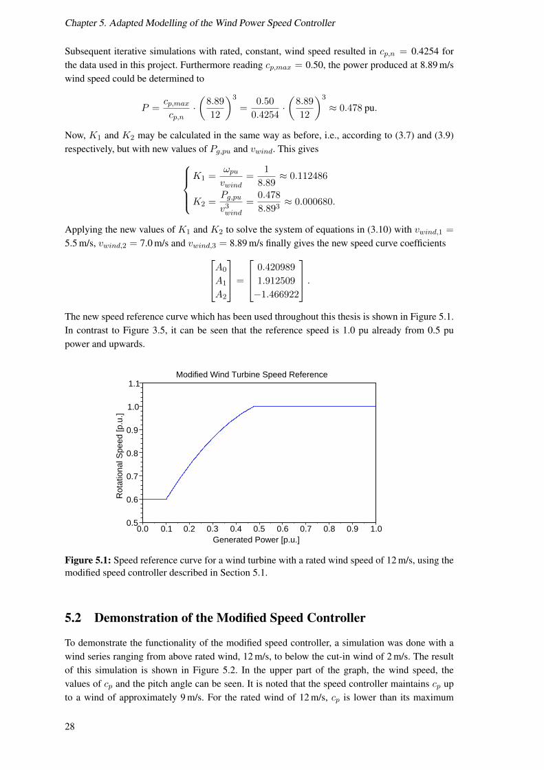
1.912509
−1.466922
.The new speed reference curve which has been used throughout this thesis is shown in Figure 5.1.In contrast to Figure 3.5, it can be seen that the reference speed is 1.0 pu already from 0.5 pupower and upwards.
0.5
0.6
0.7
0.8
0.9
1.0
1.1
0.0 0.1 0.2 0.3 0.4 0.5 0.6 0.7 0.8 0.9 1.0
Modified Wind Turbine Speed Reference
Generated Power [p.u.]
Rot
atio
nal S
peed
[p.u
.]
Figure 5.1: Speed reference curve for a wind turbine with a rated wind speed of 12 m/s, using themodified speed controller described in Section 5.1.
5.2 Demonstration of the Modified Speed Controller
To demonstrate the functionality of the modified speed controller, a simulation was done with awind series ranging from above rated wind, 12 m/s, to below the cut-in wind of 2 m/s. The resultof this simulation is shown in Figure 5.2. In the upper part of the graph, the wind speed, thevalues of cp and the pitch angle can be seen. It is noted that the speed controller maintains cp upto a wind of approximately 9 m/s. For the rated wind of 12 m/s, cp is lower than its maximum
28

5.2. Demonstration of the Modified Speed Controller
value, namely around 0.42. The pitch angle behaves like expected and mainly pitches the bladesfor strong winds, i.e., above rated wind. There is also a deflection of the pitch angle at about 370seconds, when the wind increases from 11 to 12 m/s. Normally, this would not be expected but itis a result of the turbine speed deviating from its reference value due to the wind speed change.This causes an input ∆ω to the pitch controller which is large enough to result in a pitching ofthe blades, cf. Figure 3.6. Nonetheless, in the lower part of the graph, it is seen that the turbinespeed follows the reference value in a satisfactory way. It returns to its reference value quicklyafter having deviated from it during wind speed changes. The produced power is seen to changeaccording to the wind, reaching its rated value for wind speeds of 12 m/s and above. At around1000 seconds into the simulation, the wind falls to such low values that the produced power will beso low that in turn, the turbine reference speed remains constant at its minimum value. Eventually,the turbine shuts down before 1200 seconds when the wind speed reaches the cut-in wind of 2 m/s.Lastly, comparing these simulation results with the speed reference curve in Figure 5.1, it showsthat the turbine does as expected. It reaches nominal operating speed already at approximately 220seconds when the power generation is around 0.5 pu.
0 100 200 300 400 500 600 700 800 900 1000 1100 1200
TIME SECONDS
2,0
4,0
6,0
8,0
10,0
12,0
14,0
16,0
18,0
-0,300
-0,200
-0,100
0,000
0,100
0,200
0,300
0,400
0,500
0,0
2,0
4,0
6,0
8,0
10,0
12,0
14,0
16,0
wind speed
c_p
pitch angle
0 100 200 300 400 500 600 700 800 900 1000 1100 1200
TIME SECONDS
0,300
0,400
0,500
0,600
0,700
0,800
0,900
1,000
0,300
0,400
0,500
0,600
0,700
0,800
0,900
1,000
0,00
0,20
0,40
0,60
0,80
1,00
1,20
1,40
Figure 5.2: Demonstration of the wind turbine model using the modified speed controller. Herethe wind turbine runs in an unregulated mode, i.e., it is neither frequency nor power controlled.
29

Chapter 5. Adapted Modelling of the Wind Power Speed Controller
30

Chapter 6
Results and Analysis of Frequency andActive Power Feedback Control
In this chapter, the layout of the simulated power system is first presented. Next, some of the inputdata to the implemented model is listed to clarify how the simulations have been performed. Fol-lowing that, the actual simulation results for different deloading levels and turbine control modes,namely frequency regulation (f-reg), active power feedback regulation (P-reg) and combined fre-quency and power regulation (c-reg), are presented and analysed. A brief investigation of the effecton the frequency of higher wind power penetration is made. The result chapter ends with a studyof how the wind turbine performs without regulation of the pitch controller when using the activepower feedback control.
6.1 Simulated Power System
The power system used in the simulations is an islanded system with hydro power plants and awind farm rated at 61.5 MVA or 60 MW. The hydro generators are all modelled as type 1 generatorsin SIMPOW, cf. Section 3.4, meaning that they are modelled with a field winding, one d-axisdamper winding, two q-axis damper windings and including saturation. Adding to that, they areimplemented together with PID based governors providing active frequency control, though thedroop setting of each production unit is set to 0 %. The system consists of 24 nodes, as shownin Figure 6.1. The main voltage level of the system is 150 kV and all generators are connectedthrough step-up transformers. The power flow calculation, which is run in the SIMPOW moduleoptpow, uses the generator called G1 as the swing bus. The wind power production level is set to60 MW, assuming at least nominal wind conditions.
The simulations in this chapter are primarily made with a total hydro power capacity of285 MVA spread over six generators as listed in Table 6.1. Looking at the system load, it sumsup to a total of around 203 MW and 99 MVAr. The loads are modelled as simple P and Q loads,non-frequency dependent and without inertia . This configuration gives an installed wind powershare of approximately 22 %. The exception from this set-up is found in Section 6.5 where resultsare presented for a case with 36 % installed wind power. This set-up has been emulated by dis-connecting generators G2 and G5, giving a total hydro capacity of 169 MVA. Together with thedecrease in generating capacity, the load has been decreased according to the initial loading levelof generators G2 and G5, giving a total load of 143 MW and 70 MVAr.
31

Chapter 6. Results and Analysis of Frequency and Active Power Feedback Control
N1
N2
N3
N4
N5
N6
N7N8
N9
N10
N14
N13
N11 N12
N17 N18
N15 N16
G2
G1
G3 G4 G5 G6
NG3 NG4
NG1
NG2
NG5 NG6
Figure 6.1: Topology of the simulated power system.
Table 6.1: Basic data of the generators in the simulated power system island.
Production node Rated power [MVA] Rated voltage [kV] Inertia constant H [s]G 1 25 6.6 2G 2 26 11 2G 3 27 11 2G 4 27 11 2G 5 90 16 3G 6 90 16 3
Total capacity 285
6.2 Wind Power Data
The details of the wind power modelling in SIMPOW have previously been described in Chapters3 and 5. The simulations made in this thesis use an aggregated wind farm with a rated powerof 60 MW. The aggregation is done by letting the wind farm consist of 20 3 MW wind turbinesand then following the description in Section 3.3. The only variables affected by the aggregationare the nominal power Sn, nominal turbine speed ωn and blade length R. Rfarm is calculatedby inserting nominal values into (3.9) and finding the radius from the swept area A. ωn,farm islikewise calculated by using (3.7) with nominal values inserted and then converted to rounds perminute. Finally, another important set of data is the cp(λ) curves. The ones used in this project aretaken from [2] and they are plotted in Figure 6.2. In case the pitch angle lies between one of thesecurves, SIMPOW automatically interpolates an estimated value between the relevant curves [18].
32

6.3. Comparison of Deloading Levels
beta = 0 degreesbeta = 5 degreesbeta = 10 degreesbeta = 15 degrees
0.0
0.1
0.2
0.3
0.4
0.5
0.6
0.7
0.8
0 2 4 6 8 10 12 14 16 18 20tip speed ratio lambda
c_p
Figure 6.2: cp(λ) curves used in the simulations.
6.3 Comparison of Deloading Levels
First among the results, a comparison between different deloading levels is presented. The purposeof this comparison is to introduce the effect of different pitch angle offsets. Understanding this isimportant in order to understand the other simulation results. However, the comparison made inthis thesis is not complete. It is only made under normal wind fluctuations and not in extremewind. The previous work done by AF in [20] presents a complete study on this specific topic.
The turbine deloading is accomplished by increasing the pitch angle offset β0. The defaultvalue β0 = −1 guarantees that the blades will only pitch for wind speeds greater than the nom-inal wind, i.e., when the speed deviation becomes large enough to overcome the default offset.However, giving β0 a positive value will result in the blades being pitched with this value at thebeginning of each simulation. Depending on the character of the wind series and the state of thesurrounding power system, the pitch angle may thereafter increase or decrease. The pitch off-set makes the turbine capture less wind and thereby generate less power. This non-optimal windcapture is the energy buffer that makes up the turbine deloading and causes the power curtailment.
To determine suitable deloading levels, a simulation with the unregulated wind power modeland the normal wind series was run. This set up constitutes the true Maximum Power Point Track-ing case and functions as a reference for all other simulations. The energy of the MPPT with 0◦
pitch offset was calculated. Subsequent simulations with the unregulated wind turbine were run,but this time with a positive β offset. Comparing the energy yield of each run, the 3.3◦ pitch offsetwas determined so that it would yield 95 % energy in normal wind. The 6.0◦ pitch offset was de-termined to give 80 % of the energy of the reference case, i.e., the MPPT case without deloading.These β offsets were kept in extreme wind as well, even though the energy yield at β = 6.0◦ turnsout to be somewhat higher than 80 %. The legends in the plots state which deloading level that hasbeen utilized, as well as which control concept. The one called “f-reg” is the frequency controlmethod from [20] and the one called “P-reg” is the active power feedback control which has beendeveloped in this thesis. The “P-reg” control is sometimes also called power smoothing control.
33
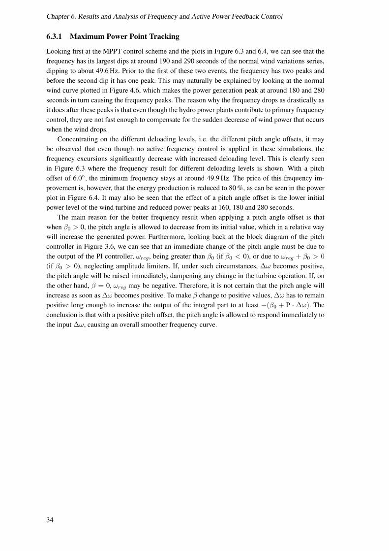
Chapter 6. Results and Analysis of Frequency and Active Power Feedback Control
6.3.1 Maximum Power Point Tracking
Looking first at the MPPT control scheme and the plots in Figure 6.3 and 6.4, we can see that thefrequency has its largest dips at around 190 and 290 seconds of the normal wind variations series,dipping to about 49.6 Hz. Prior to the first of these two events, the frequency has two peaks andbefore the second dip it has one peak. This may naturally be explained by looking at the normalwind curve plotted in Figure 4.6, which makes the power generation peak at around 180 and 280seconds in turn causing the frequency peaks. The reason why the frequency drops as drastically asit does after these peaks is that even though the hydro power plants contribute to primary frequencycontrol, they are not fast enough to compensate for the sudden decrease of wind power that occurswhen the wind drops.
Concentrating on the different deloading levels, i.e. the different pitch angle offsets, it maybe observed that even though no active frequency control is applied in these simulations, thefrequency excursions significantly decrease with increased deloading level. This is clearly seenin Figure 6.3 where the frequency result for different deloading levels is shown. With a pitchoffset of 6.0◦, the minimum frequency stays at around 49.9 Hz. The price of this frequency im-provement is, however, that the energy production is reduced to 80 %, as can be seen in the powerplot in Figure 6.4. It may also be seen that the effect of a pitch angle offset is the lower initialpower level of the wind turbine and reduced power peaks at 160, 180 and 280 seconds.
The main reason for the better frequency result when applying a pitch angle offset is thatwhen β0 > 0, the pitch angle is allowed to decrease from its initial value, which in a relative waywill increase the generated power. Furthermore, looking back at the block diagram of the pitchcontroller in Figure 3.6, we can see that an immediate change of the pitch angle must be due tothe output of the PI controller, ωreg, being greater than β0 (if β0 < 0), or due to ωreg + β0 > 0
(if β0 > 0), neglecting amplitude limiters. If, under such circumstances, ∆ω becomes positive,the pitch angle will be raised immediately, dampening any change in the turbine operation. If, onthe other hand, β = 0, ωreg may be negative. Therefore, it is not certain that the pitch angle willincrease as soon as ∆ω becomes positive. To make β change to positive values, ∆ω has to remainpositive long enough to increase the output of the integral part to at least −(β0 + P · ∆ω). Theconclusion is that with a positive pitch offset, the pitch angle is allowed to respond immediately tothe input ∆ω, causing an overall smoother frequency curve.
34

6.3. Comparison of Deloading Levels
MPPT 0 degrees deloadingMPPT 3.3 degrees deloadingMPPT 6.0 degrees deloading
49.6
49.8
50.0
50.2
50.4
50.6
50 100 150 200 250 300 350
Frequency, normal wind variations
Time [s]
Fre
quen
cy [H
z]
Figure 6.3: Frequency for different deloading levels running MPPT mode, normal wind.
MPPT 0 degrees deloading 2228 kWhMPPT 3.3 degrees deloading 2112 kWh = 95 %MPPT 6.0 degrees deloading 1792 kWh = 80 %
20
25
30
35
40
50 100 150 200 250 300 350
Power and energy, normal wind variations
Time [s]
Pow
er [M
W]
Figure 6.4: Generated power for different deloading levels running MPPT mode, normal wind.
35

Chapter 6. Results and Analysis of Frequency and Active Power Feedback Control
6.3.2 Frequency Control
Having analysed the results for different deloading levels under MPPT operation, next, the out-come when applying the frequency regulation developed by AF is shown. The relevant graph forthis evaluation is Figure 6.5 showing the frequency of the system. Looking at this plot, it can beseen that the frequency regulation clearly is effective, independent of the turbine deloading level.At 0◦ deloading the frequency curve is distinctly improved compared to the MPPT case, and at3.3◦ and 6.0◦ deloading the frequency excursions are further reduced. One may specifically lookat the time instants of approximately 190 and 290 seconds where the frequency dips are almosterased. This is due to the not so steep power derivate of the generated power when deloading theturbine. When the change in generated power is slower, the hydro generators will be able to bet-ter compensate for the decreased wind power generation. In addition, the frequency will be lessinfluenced by a decrease in the wind turbine power when the decrease takes place from a lower,i.e., deloaded, power level. The amount of produced energy is given in Table 6.2. It can be seenthat the outcome of applying frequency control to the wind farm is advantageous, since the energydecrease for 0◦ and 3.3◦ deloading is only 1 percentage point. In case of 6.0◦ deloading, the energyproduction is even equal to the unregulated case (i.e., the MPPT case).
MPPT 0 degrees deloadingf-reg 0 degrees deloadingf-reg 3.3 degrees deloadingf-reg 6.0 degrees deloading
49.6
49.8
50.0
50.2
50.4
50.6
50 100 150 200 250 300 350
Frequency, normal wind variations
Time [s]
Fre
quen
cy [H
z]
Figure 6.5: Frequency for different deloading levels running f-reg mode, normal wind.
36

6.3. Comparison of Deloading Levels
6.3.3 Active Power Feedback Control
The last comparison of deloading levels under normal wind fluctuations is done for the powerfeedback regulation developed in this thesis. Figure 6.6 shows the frequency curves for this case.Overall, the comparison shows results similar to the frequency control in the Section 6.3.2. Fromthe frequency plot, it is evident that the power feedback control effectively smooths the frequencycurve, even without turbine deloading. The dips at around 190 and 290 seconds are effectivelymitigated, and at these instances, the power smoothing regulation shows an advantage over thefrequency control in the case of no power reserve, cf. Figures 6.5 and 6.6. However, this comes atthe price of a slightly lower energy yield, 98 % instead of 99 %. Still, the energy yield of the P-regmethod is generally comparable to the f-reg method as well as to the MPPT case, cf. Table 6.2.
MPPT 0 degrees deloadingP-reg 0 degrees deloadingP-reg 3.3 degrees deloadingP-reg 6.0 degrees deloading
49.6
49.8
50.0
50.2
50.4
50.6
50 100 150 200 250 300 350
Frequency, normal wind variations
Time [s]
Fre
quen
cy [H
z]
Figure 6.6: Frequency for different deloading levels running P-reg mode, normal wind.
6.3.4 Concluding Remark - Comparison of Deloading Levels
To conclude the comparison of different deloading levels, it can be said that both the frequencycontrol and the active power feedback control clearly improve the system frequency response.The relation between higher deloading, smoother frequency and less energy production remainsthroughout normal and extreme wind variations. Table 6.2 shows a summary of the different energyyields from Section 6.3. In short, significant frequency stability improvement is possible, thoughat the drawback of less energy being produced by the wind farm.
Table 6.2: Energy yield for different pitch angle offsets and control methods in normal wind.`````````````Regulation
Pitch Offset0◦ 3.3◦ 6.0◦
MPPT 100 % 95 % 80 %f-reg 99 % 94 % 80 %P-reg 98 % 94 % 82 %
37
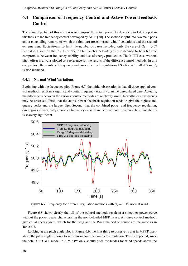
Chapter 6. Results and Analysis of Frequency and Active Power Feedback Control
6.4 Comparison of Frequency Control and Active Power FeedbackControl
The main objective of this section is to compare the active power feedback control developed inthis thesis to the frequency control developed by AF in [20]. The section is split into two main partsand a concluding remark, of which the first part treats normal wind fluctuations and the secondextreme wind fluctuations. To limit the number of cases included, only the case of β0 = 3.3◦
is treated. Based on the results of Section 6.3, such a deloading is also deemed to be a feasiblecompromise between frequency stability and loss of energy production. The MPPT case withoutpitch offset is always plotted as a reference for the results of the different control methods. In thiscomparison, the combined frequency and power feedback regulation of Section 4.3, called “c-reg”,is also included.
6.4.1 Normal Wind Variations
Beginning with the frequency plot, Figure 6.7, the initial observation is that all three applied con-trol methods result in a significantly better frequency stability than the unregulated case. Actually,the differences between the various control methods are relatively small. Nevertheless, two trendsmay be observed. First, that the active power feedback regulation tends to give the highest fre-quency peaks and the largest dips. Second, that the combined power and frequency regulation,c-reg, gives a marginally smoother frequency curve than the other control approaches, though thisis scarcely significant.
MPPT 0 degrees deloadingf-reg 3.3 degrees deloadingP-reg 3.3 degrees deloadingc-reg 3.3 degrees deloading
49.6
49.8
50.0
50.2
50.4
50.6
50 100 150 200 250 300 350
Frequency, normal wind variations
Time [s]
Fre
quen
cy [H
z]
Figure 6.7: Frequency for different regulation methods with β0 = 3.3◦, normal wind.
Figure 6.8 shows clearly that all of the control methods result in a smoother power curvewithout the power peaks characterising the non-deloaded MPPT case. All three control methodsgive equal energy yield, which for the f-reg and the P-reg method of course are the same as inTable 6.2.
Looking at the pitch angle plot in Figure 6.9, the first thing to observe is that in MPPT oper-ation, the pitch angle is down to zero throughout the complete simulation. This is expected, sincethe default FPCWT model in SIMPOW only should pitch the blades for wind speeds above the
38

6.4. Comparison of Frequency Control and Active Power Feedback Control
MPPT 0 degrees deloading 2228 kWhf-reg 3.3 degrees deloading 2100 kWh = 94 %P-reg 3.3 degrees deloading 2098 kWh = 94 %c-reg 3.3 degrees deloading 2084 kWh = 94 %
20
25
30
35
40
50 100 150 200 250 300 350
Power and energy, normal wind variations
Time [s]
Pow
er [M
W]
Figure 6.8: Power for different regulation methods with β0 = 3.3◦, normal wind.
rated wind, which is not the case in the normal wind series. Apart from that, it may be seen thatthe maximum pitch angle deflection is about 6◦. As seen when comparing the pitch angle plotto the power plot in Figure 6.8, the largest pitch angle deflections, roughly between 150 and 180seconds and between 260 and 390 seconds, correspond timewise to the periods of strong increasesin the power curve of the MPPT case. Therefore, it may be concluded that the main reason forthe smoother power curves of the regulation methods is the pitch control, which limits the turbinepower generation.
The applied control methods will also influence the turbine rotational speed. Simulation resultsdo, however, show that the difference between the MPPT case and the regulated cases is very small.
MPPT 0 degrees deloadingf-reg 3.3 degrees deloadingP-reg 3.3 degrees deloadingc-reg 3.3 degrees deloading
0
1
2
3
4
5
6
7
8
9
10
50 100 150 200 250 300 350
Pitch angle, normal wind variations
Time [s]
Ang
le [d
egre
es]
Figure 6.9: Pitch angle for different regulation methods with β0 = 3.3◦, normal wind.
39

Chapter 6. Results and Analysis of Frequency and Active Power Feedback Control
6.4.2 Extreme Wind Variations
Next, the results under extreme wind conditions, cf. Figure 4.6, are evaluated for the three differentregulation methods. First, it is noted that the frequency excursions during extreme wind fluctua-tions are, as expected, much larger than during normal wind variations. Starting with the frequencyplot in Figure 6.10, the severest frequency dips are down below 49.0 Hz. Compared to the normalwind case, this is a severe deterioration, cf. Figure 6.7. It is, however, still within the expected lev-els in an islanded system with a large share of wind power [4]. The larger frequency fluctuationsare partly due to the larger fluctuations of the extreme wind series over the normal wind series, cf.Figure 4.6, but also due to the fact that the extreme wind series lies higher in amplitude than thenormal wind series. When the wind series were filtered in [21], this was deliberately done so inorder that the extreme wind series should cause as large power and frequency fluctuations as pos-sible. Since it is higher in amplitude and the turbine power is proportional to the cube of the windspeed, any wind speed change occurring at relatively high wind speeds will cause a greater changein the turbine power and the grid frequency, than would the same wind speed change occurring atlower wind speeds.
Looking at the frequency outcome of the different control methods in Figure 6.10, it maybe seen that all three control algorithms, like in normal wind (Figure 6.7), clearly improve thefrequency curve of the system. Analogously to the normal wind case, the P-reg method givessomewhat higher frequency peaks and greater dips compared to the other methods. The f-regand c-reg methods are quite comparable, though the f-reg method seems to give slightly lowerfrequency apexes, and the c-ref method performs slightly better in case of frequency dips.
MPPT 0 degrees deloadingf-reg 3.3 degrees deloadingP-reg 3.3 degrees deloadingc-reg 3.3 degrees deloading
49.0
49.5
50.0
50.5
51.0
51.5
52.0
50 100 150 200 250 300 350
Frequency, extreme wind variations
Time [s]
Fre
quen
cy [H
z]
Figure 6.10: Frequency for different regulation methods with β0 = 3.3◦, extreme wind.
The rapid wind speed changes of the extreme wind series effect the power generation and thepitch angle deflections in a similar manner to the frequency response of the system, i.e., the fluc-tuations are quicker and larger. The maximum pitch angles will be up to 10◦. The active powerfeedback control gives a slightly higher energy yield of 92 % compared to the other two con-trol methods, cf. Table 6.3. This may, once again, be seen to correspond to the somewhat worsefrequency response of the P-reg algorithm.
40

6.4. Comparison of Frequency Control and Active Power Feedback Control
6.4.3 Concluding Remark - Comparison of Frequency Control and Active PowerFeedback Control
To sum up Section 6.4 and the comparison between different regulation methods, it can first bestated that both the frequency control algorithm and the power feedback control algorithm performwell. The results are very similar and it can merely be said that if frequency stability is the majorgoal, f-reg seems to be slightly better, given a 3.3◦ pitch angle offset. If power production is thepreferred goal, then the P-reg method should be chosen, though its advantage only appears underextreme wind conditions, cf. Table 6.3. The combined power and frequency regulation, the c-regmethod, turns out to be very similar to the two other and its use is therefore hard to motivate sinceit involves a more complex implementation.
Table 6.3: Energy yield for different wind series and control methods using a pitch angle offset of3.3◦.
`````````````RegulationWind Series
Normal Extreme
MPPT 100 % 100 %f-reg 94 % 90 %P-reg 94 % 92 %c-reg 94 % 90 %
41

Chapter 6. Results and Analysis of Frequency and Active Power Feedback Control
6.5 Comparison of Frequency Control and Active Power FeedbackControl with Increased Wind Power Share
Following the comparisons made between the different control methods in Section 6.4, this sectionintroduces the issue of increasing the wind power share in a power system and its consequenceswhen applying additional control methods. The simulations here are made with the same aggre-gated wind farm of 60 MW as previously in this chapter. The amount of hydro power generationand load is however changed to 169 MW generation capacity and 143 MW + j 70 MVAr load, asdescribed in Section 6.1. Making this change to the power system structure gives a situation wherethe wind farm constitutes approximately 36 % of the installed generating capacity. Due to the de-creased load, the loading levels of the remaining hydro generators will match previous simulations.Results are presented for normal wind, using a pitch angle offset of 3.3◦.
The only result visualized here is the frequency plot in Figure 6.11. The first observationto be made is the overall larger frequency excursions in this case compared to the system with22 % installed wind power in Figure 6.7. Comparing these two plots in detail further reveals thatshortcoming of the active power feedback control. The inferior performance of the P-ref methodwhen the frequency peaks at around 160 and 180 seconds is worsened when the wind powerpenetration increases. The result during the frequency dips at around 190 and 290 seconds issimilarly aggravated. The conclusion, therefore, is that the active power feedback control workswell with a smaller amount of installed wind power and that the advantage of the frequency controlmethod becomes more evident when increasing the wind power penetration. The result of thecombined frequency and active power feedback control is almost identical to the frequency control,though partially giving a slightly more levelled frequency curve.
MPPT 0 degrees deloadingf-reg 3.3 degrees deloadingP-reg 3.3 degrees deloadingc-reg 3.3 degrees deloading
49.2
49.4
49.6
49.8
50.0
50.2
50.4
50.6
50.8
51.0
50 100 150 200 250 300 350
Frequency, normal wind variations, 36% wind power
Time [s]
Fre
quen
cy [H
z]
Figure 6.11: Frequency for different regulation methods when increasing the wind power pene-tration, β0 = 3.3◦ and normal wind.
42

6.6. Comparison of Active Power Feedback Regulation with and without Regulated Pitch Control
6.6 Comparison of Active Power Feedback Regulation with and with-out Regulated Pitch Control
The final major evaluation that is done is an investigation of the effect of the regulated pitchcontroller and a pitch angle offset. In all of the previously presented simulation results, the windturbine is simulated using control algorithms added both to the speed controller and to the pitchcontroller. The relevant block schemes for the power smoothing regulation method are the onesgiven in Figure 4.3 and in Figure 4.4. These have so far always been used together. The aim ofthis section is to evaluate the difference between using both the regulated pitch and the regulatedspeed controller, as opposed to using the regulated speed controller together with the unregulatedpitch controller in Figure 3.6. This comparison is done exclusively for the “P-reg” concept undernormal wind conditions. To help identify the strengths and weaknesses of each configuration, thecomparison is made with β0 = 0◦ and β0 = 3.3◦. Results are shown as frequency, power and pitchangle plots.
6.6.1 0◦ Deloading
To begin with, the results for 0◦ deloading are presented. The relevant graphs here are Figures6.12, 6.13 and 6.14, showing the grid frequency, power generation and pitch angle respectively.
First, the frequency graph is studied, Figure 6.12. According to this plot it is obvious that thefrequency curve without regulated pitch controller is worse than with the regulated pitch controller.This is especially clear at the instances of frequency dips at around 190 and 290 seconds, but alsoin case of frequency apexes at around 160 and 280 seconds.
MPPT with regulated pitch, 0 degrees deloadingP-reg with regulated pitch, 0 degrees deloadingP-reg without regulated pitch, 0 degrees deloading
49.6
49.8
50.0
50.2
50.4
50.6
50 100 150 200 250 300 350
Frequency, normal wind variations
Time [s]
Fre
quen
cy [H
z]
Figure 6.12: Frequency, with and without regulated pitch controller, β0 = 0◦ and normal wind.
Second, looking at the power plot in Figure 6.13, the effect of the regulated pitch controlleris clearly seen, namely that it limits the power generation in case of power peaks. Operating thewind turbine with regulation only on the speed controller is evidently not enough to counteract thelarge power peaks.
Figure 6.14 shows the pitch angle and gives the explanation to the much better performanceof the regulated pitch controller. In case of MPPT operation, the blades are expected to remain
43

Chapter 6. Results and Analysis of Frequency and Active Power Feedback Control
MPPT with regulated pitch, 0 degrees deloading 2228 kWhP-reg with regulated pitch, 0 degrees deloading 2183 kWh = 98 %P-reg without regulated pitch, 0 degrees deloading 2221 kWh = 100 %
20
22
24
26
28
30
32
34
36
38
40
50 100 150 200 250 300 350
Power and energy, normal wind variations
Time [s]
Pow
er [M
W]
Figure 6.13: Power, with and without regulated pitch controller, β0 = 0◦ and normal wind.
unpitched, which they do. When there is no active regulation on the pitch controller, it only pitchesthe blades when the speed deviation ∆ω becomes large enough, cf. Figure 3.6. The regulated pitchcontroller, on the other hand, controls the pitch angle based on its additional input signal, cf. blockdiagram in Figure 4.4. The result of this is the much more beneficial pitch angle behaviour leadingto the better frequency stability. Note that since the turbine is operated without pitch offset, thepitch angle may not decrease from its initial position, wherefore the power generation is onlycurtailed following an increase in the generated power.
MPPT with regulated pitch, 0 degrees deloadingP-reg with regulated pitch, 0 degrees deloadingP-reg without regulated pitch, 0 degrees deloading
0
1
2
3
4
5
6
7
8
9
10
50 100 150 200 250 300 350
Pitch angle, normal wind variations
Time [s]
Ang
le [d
egre
es]
Figure 6.14: Pitch angle, with and without regulated pitch controller, β0 = 0◦ and normal wind.
44

6.6. Comparison of Active Power Feedback Regulation with and without Regulated Pitch Control
6.6.2 3.3◦ Deloading
In this subsection, the same comparison as in Section 6.6.1 is carried out, though this time with apitch angle offset of 3.3◦.
The frequency plot in Figure 6.15 shows that the frequency curve using the regulated pitchcontroller is preferable. However, comparing this plot to the one without pitch offset in Figure6.12, the difference is not as significant, neither in case of frequency dips nor peaks.
MPPT with regulated pitch, 0 degrees deloadingP-reg with regulated pitch, 3.3 degrees deloadingP-reg without regulated pitch, 3.3 degrees deloading
49.6
49.8
50.0
50.2
50.4
50.6
50 100 150 200 250 300 350
Frequency, normal wind variations
Time [s]
Fre
quen
cy [H
z]
Figure 6.15: Frequency, with and without regulated pitch controller, β0 = 3.3◦ and normal wind.
The pitch angle offset will make the power generation become smoother both in case of theregulated and the unregulated pitch controller. In both cases, the pitch angle may decrease im-mediately following a decrease in wind speed, which is not possible when operating the turbinewithout a pitch offset. The effect of this is the smaller difference between the frequency curves inFigure 6.15 compared to Figure 6.12.
6.6.3 Concluding Remark - Comparison of Active Power Feedback Regulation withand without Regulated Pitch Control
The main conclusion from Section 6.6 and the comparison between the regulated and the unregu-lated pitch controller is that the regulated pitch controller is of great importance to the frequencystability, especially when operating without pitch offset.
45

Chapter 6. Results and Analysis of Frequency and Active Power Feedback Control
46
Chapter 7
Application of Full Power ConverterWind Turbines to Power System BlackStart
One possible future application of wind power is to use it to black start power systems. In caseof a severe contingency leading to a black out, black start capable power plants are needed tobring the electric grid online again. This is done stepwise, beginning with a power plant havingblack start capabilities, which in the Nordic grid usually is a hydro power plant. Hydro stationsare advantageous for this task since they require less auxiliary power than thermal power plants.Once hydro power is available, step-up transformers and transmission lines may be energized inorder to transfer power to other bulk production units, restoring the grid step by step. In case ofno available hydro power, diesel backup generators may provide cranking power to larger powerplants. Possibly, wind turbines could also be used to black start larger production units. If so, tur-bines with fully rated power converts are preferable since they allow much better grid compliancethrough the variable speed and the converter control of active and reactive power. These turbinescould contribute to normal power generation when the electric grid functions as intended, and incase of a black out they could replace diesel generators and provide the necessary power to blackstart a larger production unit. Wind turbines are suitable thereto since they require a limited batterybackup in order to power yaw motors, blade pitch and other control systems. In order to simulatean actual black starting process, care has to be taken to include in-rush currents of transformersand high voltage lines as well as magnetization of induction motor loads. Such loads are the mostcommon auxiliary power demand of thermal power plants and are used to drive pumps and othermechanical equipment. To secure a safe and stable restoration process, both frequency and voltagehave to be controlled and kept within acceptable limits [9], [10].
In the present chapter, a much simplified version of a black start process is simulated. A smallgrid basically consisting of a wind turbine with a fully rated power converter, transformers, loss-less lines, a synchronous generator and a load, see Figure 7.1, is used in these simulations. Theintention of the analysis made in this chapter is not to be thorough as in including the electromagnetic transient phenomena of saturation and charging currents mentioned above, but rather tomake a first estimation of the feasibility of using wind power plants in this application. A secondaspect of this initial study is to see if the frequency based wind turbine control adequately handlesthese operational challenges.
47

Chapter 7. Application of Full Power Converter Wind Turbines to Power System Black Start
N1
N2
N3
N4
N5
NG1
Figure 7.1: System layout of the small power system used for simplified black start studies.
7.1 Description of the Simulated Case
In this chapter, simulation results for a few different cases, with the load in Figure 7.1 being aninduction machine, are presented. The simulations are run with the synchronous generator at busNG1 initially being connected. However, 45 seconds into the simulation, the synchronous generatoris disconnected and thereafter the wind turbine is the only production source in the grid. Thesystem is run with a single wind turbine of 3 MW and not with a whole wind farm as in Chapter 6.
7.2 Induction Machine Load
The system is simulated using an induction machine as system load. The induction machine hasa rated power of 3 MVA, i.e., almost but not exactly equal to the wind turbine rated power, whichgives slightly different per unit values of the turbine and the motor. Primarily, simulations aremade with a constant wind of 9.6 m/s, making the wind turbine produce 1.83 MW. The inductionmachine load torque has been matched to this power production in order to render a steady stateoperating point possible after the disconnection of the synchronous generator. All simulationsinvolving the induction machine load include a load torque change between 100 and 125 second,at which the load torque of the motor is linearly ramped down by 10 % from the initial steady statevalue. The load torque change implies that the system has to find a new operating point accordingto the torque speed curve of an induction machine depicted in Figure 7.2.
7.2.1 Without Frequency Control
The first simulated case has been made with an unregulated wind turbine, i.e., it includes nei-ther frequency nor active power feedback control. The wind turbine operates according to themaximum power point tracking principle and the wind is constant. Figures 7.3, 7.4 and 7.5 showthe results for the wind turbine and induction machine, as well as the grid voltage and frequency.Looking first at Figure 7.4, it can be seen that the voltage drops to a little more than 0.9 pu when thesynchronous generator is disconnected at 45 seconds. This is due to the fact that the synchronousgenerator reactive power contribution is not substituted by reactive power from the wind turbine,
48

7.2. Induction Machine Load
n
T
synchronous
speed
normal motor range
normal generator range
normal load
heavy load
Figure 7.2: Standard torque speed curve of an induction machine.
see Figure 7.5, because the turbine is generally controlled in order to maintain a unity power factorat the wind generator terminals [18]. The spikes at 45 seconds are all due to the tripping of thethe synchronous generator. The main thing to observe in these two figures is the change between100 and 125 seconds, when the motor load torque is decreased by 10 %. Since the power produc-tion of the wind turbine is constant due to the constant wind, the driving torque of the inductionmachine will initially be larger than the braking torque of the load, leading to a speed increaseof the motor, in analogy with Equation (2.1). In the simulation, the induction machine operateswithin the normal motor range of Figure 7.2, meaning that when its speed increases, its torquedecreases. Nevertheless, the product of the torque and speed, being power, remains constant andthe system finds a new equilibrium when the load torque stabilizes. The motor power is plottedwith a negative sign since the power is absorbed. Comparing the speed of the motor in Figure 7.4to the grid frequency in Figure 7.3, it is noted that both before and after the torque adjustment, theinduction machine operates in subsynchronous mode, i.e., as a motor, since the synchronous speedis proportional to the grid frequency. It is clear that the load torque change will cause an undesiredincrease in the system frequency.
40 60 80 100 120 140 160 180 200
TIME SECONDS
0,9900
1,0000
1,0100
1,0200
1,0300
1,0400
0,400
0,450
0,500
0,550
0,600
0,0
5,0
10,0
15,0
20,0
25,0
30,0
DATE 29 AUG 2012 TIME 13:21:48 JOB IM_noreg Simpow 11.0.008 Diagram:6STRI Software
wind turbine power
pitch angle
frequency
Figure 7.3: Grid frequency, wind turbine power and pitch angle using an unregulated wind turbineand an induction machine load. The synchronous generator is disconnected at 45 seconds.
49

Chapter 7. Application of Full Power Converter Wind Turbines to Power System Black Start
40 60 80 100 120 140 160 180 200
TIME SECONDS
-0,620
-0,600
-0,580
-0,560
-0,540
-0,520
-0,500
-0,480
0,9900
1,0000
1,0100
1,0200
1,0300
1,0400
-0,620
-0,600
-0,580
-0,560
-0,540
-0,520
-0,500
-0,480
0,800
0,850
0,900
0,950
1,000
1,050
1,100
1,150
1,200
DATE 29 AUG 2012 TIME 13:21:48 JOB IM_noreg Simpow 11.0.008 Diagram:7STRI Software
induction machine powerinduction machine speedinduction machine torquegrid voltage node FFORS_TG1
induction machine torque
induction machine power
induction machine speed
grid voltage node N_G1
Figure 7.4: Induction machine power, speed and torque, and grid voltage, using an unregulatedwind turbine.
40 60 80 100 120 140 160 180 200
TIME SECONDS
0,00
0,50
1,00
1,50
2,00
2,50
0,00
0,50
1,00
1,50
2,00
2,50
0,00
0,50
1,00
1,50
2,00
2,50
0,00
0,50
1,00
1,50
2,00
2,50
DATE 29 AUG 2012 TIME 13:21:48 JOB IM_noreg Simpow 11.0.008 Diagram:3STRI Software
S Y N C FFOR S _T G1 P P O W E R M W
S Y N C FFOR S _T G1 Q P OW E R M v a r
S Y N C FP CW T _GE N P P O W E R M W
S Y N C FP CW T _GE N Q P OW E R M v a r
synchronous generator active power [MW]
synchronous generator reactive power [MVAr]
wind turbine active power [MW]
wind turbine reactive power [MVAr]
Figure 7.5: Active and reactive power generation of the synchronous generator and the windturbine, using the an unregulated wind turbine and an induction machine load.
50
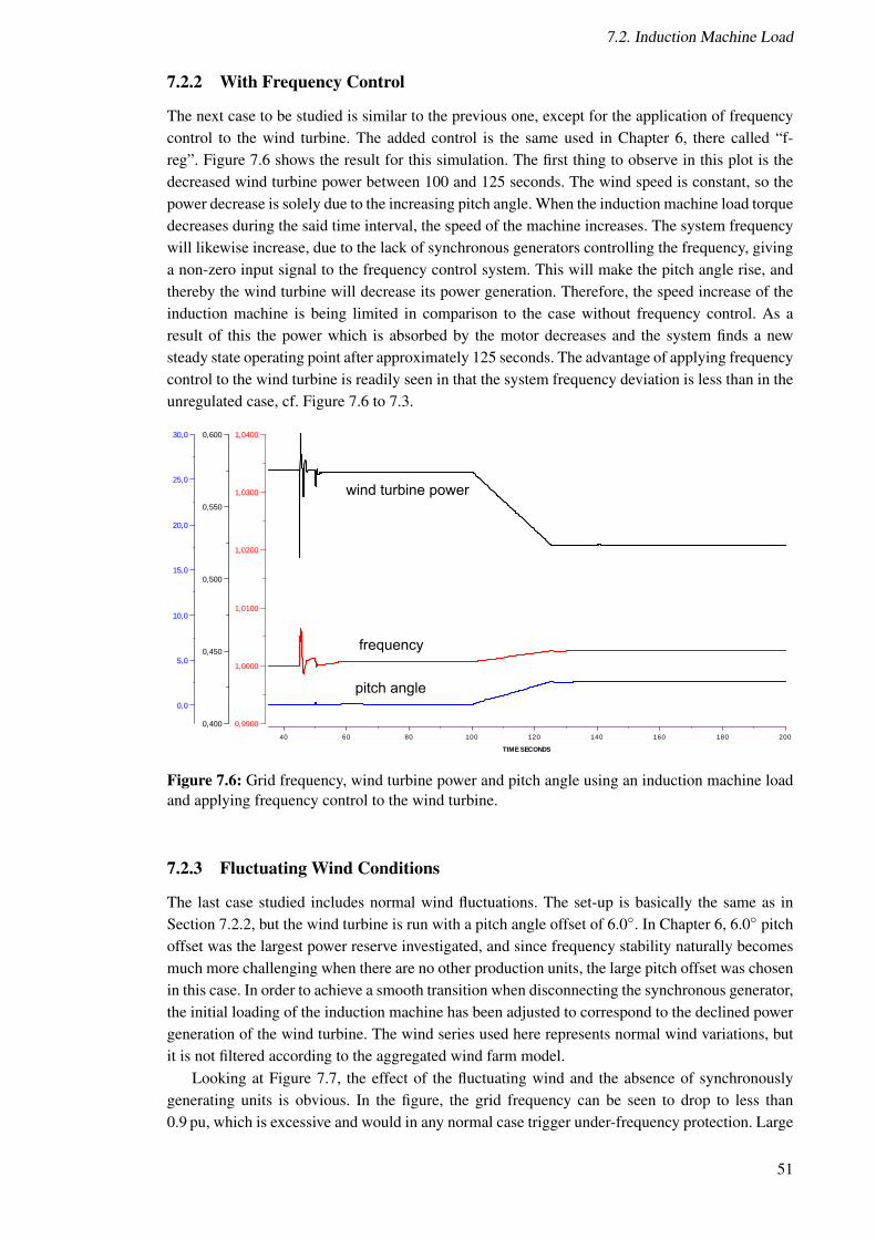
7.2. Induction Machine Load
7.2.2 With Frequency Control
The next case to be studied is similar to the previous one, except for the application of frequencycontrol to the wind turbine. The added control is the same used in Chapter 6, there called “f-reg”. Figure 7.6 shows the result for this simulation. The first thing to observe in this plot is thedecreased wind turbine power between 100 and 125 seconds. The wind speed is constant, so thepower decrease is solely due to the increasing pitch angle. When the induction machine load torquedecreases during the said time interval, the speed of the machine increases. The system frequencywill likewise increase, due to the lack of synchronous generators controlling the frequency, givinga non-zero input signal to the frequency control system. This will make the pitch angle rise, andthereby the wind turbine will decrease its power generation. Therefore, the speed increase of theinduction machine is being limited in comparison to the case without frequency control. As aresult of this the power which is absorbed by the motor decreases and the system finds a newsteady state operating point after approximately 125 seconds. The advantage of applying frequencycontrol to the wind turbine is readily seen in that the system frequency deviation is less than in theunregulated case, cf. Figure 7.6 to 7.3.
40 60 80 100 120 140 160 180 200
TIME SECONDS
0,9900
1,0000
1,0100
1,0200
1,0300
1,0400
0,400
0,450
0,500
0,550
0,600
0,0
5,0
10,0
15,0
20,0
25,0
30,0
wind turbine power
pitch angle
frequency
Figure 7.6: Grid frequency, wind turbine power and pitch angle using an induction machine loadand applying frequency control to the wind turbine.
7.2.3 Fluctuating Wind Conditions
The last case studied includes normal wind fluctuations. The set-up is basically the same as inSection 7.2.2, but the wind turbine is run with a pitch angle offset of 6.0◦. In Chapter 6, 6.0◦ pitchoffset was the largest power reserve investigated, and since frequency stability naturally becomesmuch more challenging when there are no other production units, the large pitch offset was chosenin this case. In order to achieve a smooth transition when disconnecting the synchronous generator,the initial loading of the induction machine has been adjusted to correspond to the declined powergeneration of the wind turbine. The wind series used here represents normal wind variations, butit is not filtered according to the aggregated wind farm model.
Looking at Figure 7.7, the effect of the fluctuating wind and the absence of synchronouslygenerating units is obvious. In the figure, the grid frequency can be seen to drop to less than0.9 pu, which is excessive and would in any normal case trigger under-frequency protection. Large
51

Chapter 7. Application of Full Power Converter Wind Turbines to Power System Black Start
variations also occur in the induction machine power, torque and speed. An interesting obser-vation is the pitch angle in Figure 7.7, which can be seen to rapidly decrease to zero after thedisconnection of the synchronous generator at 45 seconds. Between 85 and 160 seconds into thesimulation, the pitch angle is down to zero. It may also be seen that the unmistakable change in thegrid frequency commences at around 85 seconds, simultaneous to the blades being completely un-pitched. The conclusion therefore, is that an even larger turbine deloading possibly could mitigatethe frequency deviation and the overall unstable behaviour of the induction machine. This wouldof course mean that more wind is being spilled, which, however, is unimportant in the process ofsystem restoration.
40 60 80 100 120 140 160 180 200
TIME SECONDS
0,860
0,880
0,900
0,920
0,940
0,960
0,980
1,000
1,020
0,100
0,150
0,200
0,250
0,300
0,350
0,400
0,450
0,500
0,0
5,0
10,0
15,0
20,0
25,0
30,0
DATE 29 AUG 2012 TIME 14:18:01 JOB IM_normal_fregf Simpow 11.0.008 Diagram:6STRI Software
frequencywind turbine powerpitch angle
wind turbine power
pitch angle
frequency
Figure 7.7: Grid frequency, wind turbine power and pitch angle using an induction machine loadand applying frequency control to the wind turbine under normal wind fluctuations.
7.2.4 Concluding Remark - Induction Machine Load
The simulation results in this section show the feasibility of applying wind turbine frequencycontrol to very small power systems. Frequency excursions are effectively limited, ensuing fromthe wind turbine being able to meet the load torque change of the induction machine. However,fluctuating wind conditions put extended demands on the available power reserve of the windturbine.
52

Chapter 8
Conclusions
This thesis has shown that there exist good possibilities to control wind turbines in order to in-crease frequency stability of a power system. An active power feedback control which smooths thepower generation has been developed. This control method has been compared to the frequencycontrol developed by AF in [20]. According to the results in Chapter 6, they both enhance fre-quency stability. The frequency control is shown to be superior when the wind power penetrationexceeds approximately 25 % of the total system generation capacity, making frequency controlthe preferable method when increasing the wind power share. It is also shown that a pitch angleoffset, or more generally, a power reserve, may contribute to better frequency stability without theimplementation of an additional control strategy. Thus, in case of fluctuating wind, a pitch angleoffset can in itself achieve a smoother power generation and thereby a smoother grid frequency.Operating a wind turbine with a power reserve will always result in energy – and revenue – beingspilled. Requiring wind turbines to participate in frequency control will therefore result in a trade-off between frequency stability and energy production. The exact amount of turbine deloadinghas to be decided by each wind farm operator in collaboration with the TSO, based on the powersystem structure, applicable grid codes and possible reimbursement agreements.
The frequency control method has the advantage of being intuitive. Its response to frequencyfluctuations is natural and immediate. The active power feedback control, on the other hand, isnot as straight forward. It may, for example, happen that the frequency falls below 50 Hz and thatthe power set point remains below the actual generation level for a certain time. In such a case,the power feedback regulation will drive the turbine production in a direction contrary to whatis desired, worsening the frequency deviation. In comparison to the frequency control, the powerfeedback control is a less intuitive way of controlling the frequency. The main disadvantage is thatit does not directly control the frequency but only indirectly through the control of the generatedpower. Therefore, it becomes more dependent on other generating units to provide true frequencycontrol in order to make the generation follow the load changes.
The active power feedback control was demonstrated in Section 6.6 to be highly dependent onthe input of the additional control signal to the pitch controller. Due to the similar appearances ofthe power and pitch angle graphs for the frequency and the power based control methods in theresult chapter, the same conclusion is likely to hold for the frequency based method as well. Theresults indicate, therefore, that the main component in a successful turbine control is to utilize thepitch control system.
As stated in the beginning of Chapter 7, the investigations made therein are of a much sim-plified case which in many aspects does not represent a real black start process, lacking first andforemost the component energization. Nonetheless, the simulations made with an induction motorload identifies the need for some kind of frequency control, e.g. when driving motors in the start-up
53

Chapter 8. Conclusions
process of a thermal power plant. The frequency control algorithm was demonstrated to providesuch control ability, enabling wind turbines to supply motor loads under these circumstances. Itwas also shown that when the wind turbine is subjected to varying wind conditions, the frequencystability becomes much more difficult to preserve, requiring a large power reserve through greaterturbine deloading.
8.1 Outlook
In this thesis, an aggregated wind farm model has primarily been used. Such an aggregation sim-plifies the modelling and especially the computational cost of the simulations. As a drawback, italso simplifies the behaviour of a wind farm. To achieve more detailed results, simulations withindividual turbines would be preferable to be able to study the frequency response in-depth. An-other aspect which has has been left out in this work is that of voltage stability. When dealing withthe integration of large wind power shares, voltage stability also has to be considered and studied.How is, for example, the voltage stability margins affected by the implementation of wind powerfrequency control?
An interesting future work regarding frequency control is to quantify the required deloadinglevels of wind turbines in order to meet grid code demands. In line with such an investigation, itwould be beneficial to investigate the parameter selection of the frequency control algorithm inorder to optimize it further. The aim of such an optimization could be to increase the energy yieldfor a given deloading level, without affecting the frequency stability negatively.
Regarding the issue of applying wind turbines to power system restoration and black startprocesses, it is undoubtedly necessary to create wind power models valid at the time scale ofelectromagnetic phenomena. In the process of black starts, energization of transformers and trans-mission lines put extraordinary requirements on the generating units, making these events a testwhich wind turbines have to stand to constitute an alternative in black starts.
54

References
[1] T. Ackermann, Ed., Wind Power in Power Systems. Chichester, England: John Wiley &Sons, Ltd, 2005.
[2] H. A. L. Carballido, “Control of a wind turbine equipped with a variable rotor resistance,”Master’s thesis, Chalmers University of Technology, Goteborg, Sweden, 2009.
[3] R. Carriveau, Ed., Fundamental and Advanced Topics in Wind Power. Rijeka, Croatia:InTech, 2011.
[4] Voltage Characteristics of Electricity Supplied by Public Distribution Networks, CENELECEuropean Standard EN 50160:2007, Sep. 2007.
[5] Chowdhury, B.H. and Ma, H.T., “Frequency regulation with wind power plants,” in Powerand Energy Society General Meeting - Conversion and Delivery of Electrical Energy in the21st Century, 2008 IEEE, july 2008, pp. 1–5.
[6] Conroy, J.F. and Watson, R., “Frequency Response Capability of Full Converter Wind Tur-bine Generators in Comparison to Conventional Generation,” Power Systems, IEEE Trans-actions on, vol. 23, no. 2, pp. 649–656, may 2008.
[7] Elteknik, Department of Energy and Environment, Chalmers University of Technology,Gothenburg.
[8] Network Code for Requirements for Grid Connection applicable to all Generators, ENTSO-E working draft, Rev. January 24, 2012, Brussels, Belgium.
[9] Feltes, J.W. and Grande-Moran, C., in Power and Energy Society General Meeting - Conver-sion and Delivery of Electrical Energy in the 21st Century, 2008 IEEE.
[10] J. Glover, M. Sarma, and T. Overbye, Power System Analysis and Design, 4th ed. Stamford,USA: CENGAGE Learning, 2008.
[11] K. Kleinekorte, “Grundlagen der Systemfuhrung im Transportnetz,” lecture notes, RWTHAachen University, Germany, 2010.
[12] P. Kundur, Power System Stability and Control, N. J. Balu and M. G. Lauby, Eds. NewYork, USA: McGraw-Hill, 1994.
[13] E. Loukarakis, I. Margaris, and P. Moutis, “Frequency Control Support and ParticipationMethods Provided by Wind Generation,” in Electrical Power Energy Conference (EPEC),2009 IEEE, oct. 2009, pp. 1–6.
[14] J. Machowski, J. W. Bialek, and J. R. Bumby, Power System Dynamics Stability and Control,2nd ed. Chichester, United Kingdom: John Wiley & Sons, Ltd, 2008.
55
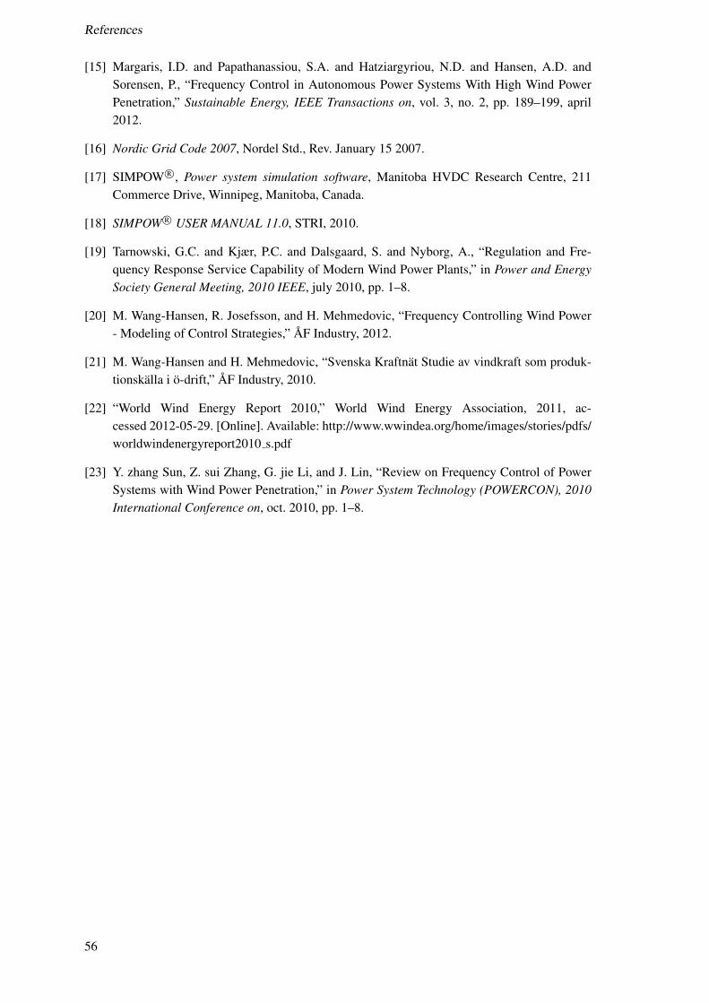
References
[15] Margaris, I.D. and Papathanassiou, S.A. and Hatziargyriou, N.D. and Hansen, A.D. andSorensen, P., “Frequency Control in Autonomous Power Systems With High Wind PowerPenetration,” Sustainable Energy, IEEE Transactions on, vol. 3, no. 2, pp. 189–199, april2012.
[16] Nordic Grid Code 2007, Nordel Std., Rev. January 15 2007.
[17] SIMPOW R©, Power system simulation software, Manitoba HVDC Research Centre, 211Commerce Drive, Winnipeg, Manitoba, Canada.
[18] SIMPOW R© USER MANUAL 11.0, STRI, 2010.
[19] Tarnowski, G.C. and Kjær, P.C. and Dalsgaard, S. and Nyborg, A., “Regulation and Fre-quency Response Service Capability of Modern Wind Power Plants,” in Power and EnergySociety General Meeting, 2010 IEEE, july 2010, pp. 1–8.
[20] M. Wang-Hansen, R. Josefsson, and H. Mehmedovic, “Frequency Controlling Wind Power- Modeling of Control Strategies,” AF Industry, 2012.
[21] M. Wang-Hansen and H. Mehmedovic, “Svenska Kraftnat Studie av vindkraft som produk-tionskalla i o-drift,” AF Industry, 2010.
[22] “World Wind Energy Report 2010,” World Wind Energy Association, 2011, ac-cessed 2012-05-29. [Online]. Available: http://www.wwindea.org/home/images/stories/pdfs/worldwindenergyreport2010 s.pdf
[23] Y. zhang Sun, Z. sui Zhang, G. jie Li, and J. Lin, “Review on Frequency Control of PowerSystems with Wind Power Penetration,” in Power System Technology (POWERCON), 2010International Conference on, oct. 2010, pp. 1–8.
56