a new version of elman neural networks for dynamic systems ... · a new version of elman neural...

Journal of Engineering Sciences, Assiut University, Vol. 34, No. 2, pp. 487-508, March 2006

A NEW VERSION OF ELMAN NEURAL NETWORKS FOR DYNAMIC SYSTEMS MODELING AND CONTROL

_____________________________________________________________________________

Dr. Hamdi A. Awad

Department of Industrial Electronics and Control Engineering, Faculty

of Electronic Engineering, Menouf, 32952, Menoufia University, Egypt.

[email protected]

(Received December 28, 2005 Accepted February 6, 2006)

ABSTRACT – Elman network is a class of recurrent neural networks

used for function approximation. The main problem of this class is that its

structure has a set of global sigmoid functions at its hidden layer. That

means that if the operating conditions of a process be identified, are

changed the function approximation property of the network is degraded.

This paper introduces a new version of the Elman network named Elman

Recurrent Wavelet Neural Network (ERWNN). It merges the multi-

resolution property of the wavelets and the learning capabilities of the

Elman neural network to inherit the advantages of the two paradigms and

to avoid their drawbacks. Stability and convergence property is proven

for the proposed network. The paper also develops a model reference

control scheme using the proposed ERWNN. The proposed scheme

belongs to indirect adaptive control schemes. The dynamic back

propagation (DBP) algorithm is employed to train both the two networks

structured for the indirect control scheme. This paper derives also the

plant sensitivity for adjusting the parameters of the developed controller.

The advantages of this new version of ERWNN in modeling and

controlling time intensive dynamic processes, are reflected in our

simulation results.

KEY WORDS: Recurrent neural network , wavelets, respiratory

systems.

1. INTODUCTION

The nonlinear function mapping properties of neural networks are central to their use

in modeling and controlling dynamic systems [1–4]. In general, neural networks can be

classified according to their structures into feedforward networks include the multi-

layer perceptron (MLP) [5], and recurrent networks include the Elman network [6].

They can also be classified according to their learning algorithms include supervised

learning [5], unsupervised learning [7] and [8], and reinforcement learning [9]. The

Elman recurrent neural network (ERNN) is a type of recurrent networks that has a wide

range of applications [10], [11], and [12]. Training the self feedback Elman network

with dynamic backpropagation (DBP) algorithm was proposed by Pham and Liu [13].

487

mailto:[email protected]

Hamdi A. Awad ________________________________________________________________________________________________________________________________

488

Unlike, the basic Elman network trained by the standard backpropagation (BP)

algorithm, the modified Elman trained by DBP was able to model high-order dynamic

systems.

Recently, a set of neural networks are structured based on the concepts of the

wavelet transform. There are two kinds of Wavelet Neural Networks (WNNs), one

with fixed dilation and translation parameters, and the other with adjustable dilation

and translation parameters [14] and [15]. The latter realizes the multiresolution

property that is very useful for function approximation purposes. The wavelets with

coarse resolution can capture the global behavior (low frequency) easily, while the

wavelets with fine resolution can capture the local behavior (higher frequency). The

performance of a model-based control system depends strongly on the accuracy of the

process model used. Many real-time processes have complex, uncertain and non-linear

dynamics and so it is difficult to model them mathematically. Because of the function

approximation ability of neural networks, much research has been conducted on

adapting them for modeling and controlling dynamic systems [4] and [11].

Feedforward neural networks such as MLP and Radial Basis Function (RBF) networks

usually does pose a serious problem when it is employed for modeling purposes. This

problem can be summarized as follows. If a feedforward network is adopted for the

modeling task, then we should know the number of delayed input and output in

advance, and feed them as a taped line to the network input. The exact structure of a

dynamic system is usually unknown. Besides much taped delayed lines increase the

dimension of the input vector that results a large network size. To deal with this

problem, interest in using recurrent networks e. g. ERNN for processing dynamic

systems has been steadily growing in recent years, [16] and [17].

This paper focuses on the Elman recurrent neural network, ERNN, to overcome the

structure identification problem of the feedforward networks mentioned above. The

main drawback of using the original ERNN is that it has global sigmoid functions at its

hidden layer. That means that if the operating conditions of a process to be modeled are

changed, the function approximation property of the Elman network is degraded as

mentioned previously. This paper merges the multi-resolution property of the wavelets

and the learning capabilities of the Elman network to overcome the limitations of

ERNN on modeling and controlling dynamic systems. That results a new version of

Elman network named ERWNN that has a universe of discourse covered by a set of

local wavelets instead of global sigmoid functions. This is our first motivation. Unlike

the traditional Elman recurrent network ERNN [6], the proposed ERWNN has the

advantages of better local accuracy, generalization capability and fast convergence as

reflected from our simulation results.

This paper also introduces the proposed ERWNN for controlling dynamic systems. It

describes a design method for a model reference control structure using the proposed

ERWNN. In this structure, two ERWNNs are employed, one is a controller named

(ERWNNC) and the other is an identifier called ERWNNI that provides information

about the plant be controlled to the former. This scheme is named ERWNN-based

indirect control (ERWNN-ICS). The paper derives the plant sensitivity for adjusting

the parameters of the controller. The paper also employs the DBP to train both the two

networks of the proposed scheme and applies it for controlling time intensive

processes.

A NEW VERSION OF ELMAN NEURAL NETWORKS FOR…. ________________________________________________________________________________________________________________________________

489

Controlling of the oxygen delivery to mechanically ventilated hypoxic patients is a

time intensive process that must balance adequate tissue oxygenation against possible

toxic effects of oxygen exposure [18] and [19]. Although many researches have been

conducted for oxygenation of newborn patients, few researches are carried out for

adults. The proposal scheme has been applied to control the oxygen delivery for adults

patients. Controlling this process using conventional proportional plus integral (PI)

controller needs empirical adjustments for the controller parameters. It means that if

the operating conditions of the controlled plant is changed, these parameters should be

readjusted. A multi-model adaptive controller (MMAC) [21] and feedforward fuzzy

neural network-based indirect control scheme (FNN-ICS) [22], were introduced for

controlling this process, however satisfied results have not been achieved. This paper

employs this time intensive nonlinear process to test the proposed ERWNN-ICS.

Compared with PI, MMAC controllers and FNN-ICS, best results were achieved using

the developed ERWNN-ICS.

The motivations of this paper can be concluded as follows:

Development a new version of ERNN named ERWNN

Deriving the DBP algorithm to train the proposed ERWNN

Testing the stability and convergence of the proposed ERWNN

Development an indirect control scheme based on the proposed ERWNN

named ERWNN-ICS

Deriving the plant sensitivity to adjusting the parameters of the developed

ERWNN-ICS

The rest of the paper is organized as follows. Section 2 describes the proposed

ERWNN and its training algorithm. Section 3 depicts the modeling simulation results

using both the ERNN and the ERWNN. Section 4 details the modeling and controlling

of dynamic systems using the proposed indirect control scheme. Training both the two

networks of the proposed indirect control scheme is described in section 5. Simulation

results on modeling and controlling the respirator dynamic system are depicted in

section 6. Section 7 concludes the paper by summarizing the contributions made.

2. ElMAN RECURRENT WAVELET NEURAL NETWORK

This section details wavelet transform. It describes the structure and training algorithm

of the introduced ERWNN and derives the DBP algorithm to adapt the parameters of

the proposed network.

2.1. Wavelet Transform

Unfortunately, most signals encountered in practice, are non-stationary. Such signal

requires a time-frequency representation rather just a time or frequency representation.

In other words, technologies based on Fourier Transform (FT) or even its

modifications still suffer from a set of drawbacks. That is that FTs are not able to

analysis or approximate signals with both sharp transitions and slowly varying spectra.

Authors who did not realize this fact blindly build their technologies based on FTs.

Besides, technologies that depend on FT are quadratic or nonlinear in nature with

Hamdi A. Awad ________________________________________________________________________________________________________________________________

490

highly computation demand. Wavelet transform is the only linear transform that can

analysis or approximate stationary and/or non-stationary signals at varying resolutions.

The basic concepts about wavelet transforms that are relevant to this paper are

briefly recalled. The coherent states g(p,q)

all have the same envelope function g, which

is translated by the amount q, and “filled in” with oscillations with frequency p [23].

Wavelets are similar to the g(p,q)

in that they also constitute a family of functions

derived from an single function, and indexed by two labels, one for position, b, and the

other for frequency, a. That is.

a

bxhaxh ba )2/1(),( )( (1)

where h is a square integral function such that.

dyyhyh

c21

)(ˆ (2)

and Rba , and 0a . If h has some decay at infinity, then (2) is equivalent to the

requirement 0)( dxxh . Compared with the coherent state g(p,q)

, wavelets will be a

better tool in situations where better time-resolution at higher frequencies, 1a , than

at low frequencies, 1a . It is clear that the major different between short-time

(windowed) FT and wavelet transform is that, in the latter high frequency components

are studied with sharper time resolution than low frequency components.

The link between wavelets and neural networks was introduced by [24]. In general, a

set of vectors Jjj , in Hilbert space H for which the sums 2

Jj

j f,Ψ yield upper

and lower bounds for the norm 2

f , is called a frame. Given a frame NM , in the

Hilbert space H , for any function Hf , f can be decomposed in terms of the frame

elements as follows [15]:

)(,)(,

1 xΨΨSfxf M,NqZNM

M,N

(3)

where S is the frame operator HH and NM , is defined below:

)(,

)(,

)(,

)( ...2

2

221

1

11, q

q

qqNM x

bax

bax

bax (4)

q

T

q

T bbbNaaaM ,,,,,,, ...... 2121 , )(, i

xi

ib

ia

can be generated by dilating and

translating the mother wavelet as will be shown in section B. The parameters ai and bi

are the dilation and translation respectively.

In most practical applications, the function of interest have finite support, therefore it

is possible to truncate infinite number of wavelet frames in (3) to reconstruct the

function f as follows:

)()(,

, xΨwxf M,N

Q

NMnM (5)


491

where M,NNM ΨSfw 1

, , and Q is the total number of wavelet function selected. This

equivalent to the wavelet neural network introduced by [24]. Initialization and wavelet

networks were described in [25] and [26].

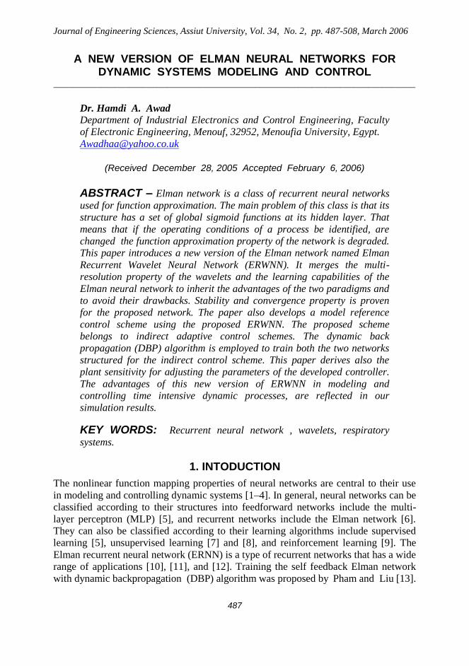
2.2. Structure of ERWNN

The structure of the proposed ERWNN is similar to the structure of ERNN that is

described in [13]. The first motivation of this paper is that it introduces the

multiresolution property of the wavelets to the ERNN by replacing the sigmoid

function at its hidden layer with a set of wavelet functions defined in (6) as depicted in

Fig. 1. The idea of employing wavelets to neural networks described in section A, was

borrowed to construct our ERWNN. The novelty of the proposed network can be

concluded as follows:

Converting the ERNN from global-support (i.e. sigmoid functions) network, ERNN, to

local-support (wavelets) network, ERWNN, results a universal tool for function

approximation as will be shown in section 3. This is due to the use of a higher

resolution of the space when the data are dense, and a lower resolution when data are

sparse.

Merging the multi resolution property of the wavelets to the ERNN, keeps the number

of the hidden/context layer approximately six for a complex process. In other words, to

obtain similar RMS values using both the two networks, the number of the

hidden/context units should be increased using the ERNN compared with the proposed

ERWNN.

Referred to Fig. 1, it can be seen that the proposed network, in addition to the input,

the hidden units and the output unit, the context units, there are also the link weights.

These weights link, respectively, the input / hidden units, the context / hidden units,

and the hidden / output units. The function of each unit at a layer in the proposed

ERWNN can be described as follows:

Layer-1: The input unit at this layer is only a buffer unit, which passes the signals with

out changing them.

Layer-2: Instead of using sigmoid functions [6] at the hidden layer of the traditional

ERNN, this paper proposes that each unit in the hidden layer implements the

multidimensional wavelets defined in (6):

n

iij x

ih

1)( (6)

where

ia

ib

iv

ix

, vi is i

th input to a hidden unit, (.)

ih is the i

th daughter wavelet

generated by a translation bi, and dilation ai from a mother wavelet (.)h . The

employed mother wavelet is:

0,)exp()1()(22

axxxh (7)

It also proposes the dilation parameter of the wavelets defined in (6) to link the

hidden and the context units as shown in Fig. 1 and the weights of the traditional

network are considered as a scaling parameters.

Hamdi A. Awad ________________________________________________________________________________________________________________________________

492

Self feedback links

α α

a a

…

…

The input unit

u(k)

The context

units xc(k)

The hidden

units x(k)

The output unit

y(k)

Fig. 1. The modified ERWNN.

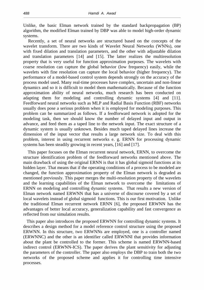
Layer-3: This layer represents the final output of the network. At a specific time k, the

previous activations of the hidden units (at time k-1) and the current input (at time k)

are used as inputs to the hidden units. At this stage, the network acts as a feedforward

network and propagates theses inputs forward to produce the output similar to the

traditional ERNN. This shows that the proposed ERWNN is an approximate realization

of ERNN. The function of each unit at a specific layer in the proposed ERWNN is

described as follows:

The input of a hidden unit at the hidden layer is:

)()1()( ,, kkk xwvc

j

x

jiji (8)

)()1()(1, kukk wvu

ii (9)

where j = 1,…,n , and i=1,2… ,n. Let l=1,2,...,n+1.

The output of a hidden unit at the hidden layer is:

2

,

,,

2

,,

,,

)(*)

)(1())((

li

lili

i

lili

lilia

kEXP

kkv

bv

a

bvh (10)

where l = 1,….,n+1

))(()( ,,

1

1

kvk lili

n

li hx

(11)

The context unit output is:

)1()1()( , kkk xxaxc

jiji

c

j (12)

The final output of the network is:


493

n

ii

n

ii

y

i

k

kk

ky

x

xw

1

1

)(

)()1(

)( (13)

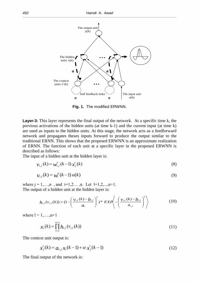
2.3. Training of the ERWNN

This paper derives the DBP algorithm to train the proposed self feedback ERWNN.

This is our second motivation in this paper. In this case the feedback vector,

)}({)( kk xxc

j

c , is )1()1(, kxkxa c

jjji , which is a function of

)2()2()2()2( kukkxk wwux . Therefore, )(kx c

j depends on the weights of the

previous time instants. When an input-output pair, (u(k),yd(k)), is presented to the

network at time k, the error function at the network output defined in (14) can be

minimized to obtain the best solution from a set of given solutions. Accordingly, the

weights are updated using DBP algorithm at each time step k as follows:

2

)()(2

1kykyE dk (14)

where yd(k) and y(k) are the desired and the actual outputs respectively.

)1(

)(*

)()1(

k

ky

kyk w

E

w

Ey

i

k

y

i

k

n

ii

i

d

k

xkyk

x

y

1

)(

*))()(( (15)

)1(

)(*

)(

)(*

)()1(

k

k

k

ky

kyk w

x

x

E

w

Eu

i

i

i

k

u

i

k (16)

2

1

11

)(

)()1(*)(

n

ii

n

ii

y

l

y

l

n

ii

ik

kwkwk

x

y

x

xx (17)

According to the above derivatives (16) becomes:

n

lu

i

lii

lili

i

du

i

k

kw

kvhkvh

x

ykyky

kw

E

1

,1,

,,

)1(

))(())((**))()((

)1(

where, )(*)(

))((

)1(

)(*

)(

))((

)1(

)(

1,

,1,1,

1,

,1,1,ku

k

kv

k

k

k

kv

k

k

v

h

w

v

v

h

w

h

i

lii

u

i

i

i

lii

u

i

i

2

,

,1,

2

,

,1,

2

,

,1,

1,

,1,

)(

)()(*

)(*

)(2*2

)(

))((

k

kkEXP

kk

k

kv

a

bv

a

bv

a

bv

v

h

li

lii

li

lii

li

lii

i

lii (18)

)1(

)(*

)(

)(*

)()1( ,,

k

k

k

ky

kyk w

x

x

E

w

Ex

ji

i

i

k

x

ji

k

)1(

)(**))()((

,

k

k

x

ykyk

w

xy

x

ji

i

id

(19)

Hamdi A. Awad ________________________________________________________________________________________________________________________________

494

1

1,

,

,

,,

,,

1

1,

,,

,,

, )1(

)(*

)(

))((*))((

)1(

))((*))((

)1(

)( n

jll

x

ji

ji

ji

jiji

lili

n

jll

x

ji

jiji

lilix

ji

i

k

k

k

kvkv

k

kvkv

k

k

w

v

v

hh

w

hh

w

x

1

1,

,,

,, )(*)(

))((*))((

n

jll

c

j

ji

jiji

lili kk

kvkv x

v

hh (20)

The variable )(kx c

j depends on the weights of the previous time instants, w(k-2).

Accordingly, substituting (20) into (12), results (See the appendix ):

)2(

)1(*)1(*)(*

)(

))((*))((

)1(

)(

,

,

1

1,

,,

,,

,

k

kkk

k

kvkv

k

k

w

xxa

v

hh

w

xx

ji

i

iji

n

lji

jiji

lilix

ji

i (21)

and )(

))((

,

,,

k

kv

v

h

ji

jiji

can be computed as (18).

For the readers who are interested, they will discovered that the term)2(

)1(*

,

k

k

w

xx

ji

i in

(20) is equivalent to )2(

)1(*)1(*

)(

))((*))((

,

,

1

1,

,,

,,

k

kkw

k

kvkv

w

x

v

hh x

ji

ix

li

n

lji

jiji

lili using the

DBP with 0),1()( , kk xax jji

c

j. Although these two terms do not provide

exactly the same search, the former can provide an infinite impulse response. The

derivative of (14) to the translation parameter of a wavelet function, b, and to the

dilation parameter of a wavelet function, a, can be derived as follows:

)(

)(*

)(

)(*

)()( ,, k

k

k

ky

kyk b

x

x

E

b

E

ji

i

i

k

gi

k

1

1

1

1,

,,

,,)(

))((*))((**))()((

n

g

n

gjj

gi

gigi

jiji

id

k

kvkv

x

ykyk

b

hhy (22)

2

,

,,

2

,

,,

2

,

,,

,

,)(

*)(

))(*

)(2*2

)(

)( (

a

bv

a

bv

a

bv

b

h

gi

gigi

gi

gigi

gi

gigi

gi

gik

EXPkk

k

k (23)

)(

)(*

)(

)(*

)()( ,, k

k

k

ky

kyk a

x

x

E

a

E

gi

i

i

k

gi

k

1

1

1

1,

,

,)(

)(*)(*

)(

)(*))()((

n

g

n

gjj

gi

gi

ji

id

k

kk

kx

kykyk

a

hhy

(24)

where,

.1,)(

(*)(

))(*)

)(2(*2

)(

)(2

,

,,

3

,

2

,,

2

,

,,

,

,(

ng

kEXP

kk

k

k

a

bv

a

bv

a

bv

a

h

gi

gigi

gi

gigi

gi

gigi

gi

gi

for (g=1,2,…,n):


495

2

,

,,

3

,

2

,,

2

,

,,

,,,

,,3

,

,,

,

,

)((*

)(

))(

*)(

2*)()(

*))((

*2)(

)(

(

a

bv

a

bv

a

bv

a

h

gi

gigi

gi

gigi

gi

gigi

gigigi

gigi

gi

gigi

gi

gi

kEXP

k

kbkv

a

kva

a

bkv

k

k

where, )1(*)1()(

)(,

,

,

kxkw

ka

kvj

x

gi

gi

gi .

3. SIMULATION RESULTS IN MODELING DYNAMIC SYSTEMS

Simulation experiments using the proposed ERWNN were conducted on modeling

dynamic systems. Since the ERWNN is employed to perform this simulation, only

control signal is fed as input to the network. The developed DBP described above is

used to adapt the parameters of the ERWNN using the differences between the desired

and the actual outputs e(k). The RMS error as defined in (25) was computed for the

trained network using the test data.

T

k

)kyk(YdT

errorRMS1

2][][1 (25)

where Yd[k] and Y[k] respectively, are the desired and the actual outputs and T is the

number of samples during the test period.

For comparison reasons, the number of hidden/context units, which should be at

least be equal the order of the system to be modeled, was taken as six to enable the

conventional ERNN and the proposed ERWNN to model and control most practical

systems. The training times for the DBP-trained ERNN and the DBP-trained proposed

ERWNN were the same in the following simulation examples. Both the two networks

are tested using two types of processes, one is linear and the other is nonlinear.

3.1. Linear Systems Modeling

Although the proposed ERWNN with the DBP can model complex systems, it has first

been used to identify a linear system to test the soundness of the proposed network.

The third-order linear system employed in this simulation has one real pole and two

complex poles [13]:

])[()()(

2221

tStSSG (26)

Its discrete form is:

)3()2()1()3()2()1()( 321321 kuBkuBkuBkyAkyAkyAky (27)

With sampling period T=0.08 Sec. and the parameters t2=1.0, t1=2.5 and 5.2

2 ,

the coefficients of (27) are A1=2.627771, A2=-2.333261, A3=0.697676, B1=0.017203

and B2=-0.030862, B3=0.014086. The training normalized squares set of 600 data

points, was produced randomly to the system model with zero initial conditions and

Hamdi A. Awad ________________________________________________________________________________________________________________________________

496

recording the output data. After training the two networks, they were tested using a

different random set of 100 points and the responses of the conventional ERNN and the

proposed ERWNN are obtained and the RMS errors were computed using the RMS

error defined in (25). They are 4.04*10-3

and 1.38*10-3

respectively.

3.2. Non-linear Systems Identifications

The ERNN and the proposed ERWNN were also tested using a non-linear dynamic

system. The same structure used for the above linear system modeling was employed.

The nonlinear system model is [27] and [28]:

)())1(1415926.3sin(1.0

)2()))1(exp(9.03.0(

)1()))1(exp(5.08.0()(

2

2

keky

kyky

kykyky

(28)

where e(k) was a Gaussian white noise sequence with zero mean and variance equal to

0.01. A data base of 600 data points was created using (28) (initial condition: y(0)=y(k-

1) =0.1). The first 500 data were employed as training data. The last 100 data were

reserved as new data test for the trained model. Both the ERNN and the proposed

ERWNN were trained using noise e(k) as the input and y(k) as the desired output. The

DBP was employed as the training algorithm. The response of the trained two networks

to the new data are depicted in Fig. 2 and Fig. 3 and the RMS error defined in (25) was

computed for the testing data of the ERNN and the proposed ERWNN and was found

0.76 and 0.53 respectively.

Using the conventional ERNN and the proposed ERWNN with DBP algorithm,

modeling simulation RMS errors for the above experiments are listed in Table I. The

table shows that best results have been obtained using the proposed ERWNN network.

It also depicts that using the two networks to obtain similar RMS error values, e. g.

1.38*10-3

and 0.53 respectively, the number of hidden/context units of the conventional

ERNN should be increased.

-2

-1

0

1

2

500 520 540 560 580 600

Fig. 2. Response of the ERNN (the non-linear system defined in (28)).


497

-2

-1.5

-1

-0.5

0

0.5

1

1.5

2

500 520 540 560 580 600

Fig. 3. Response of the proposed ERWNN (the non-linear system defined in (28)).

Table 1: Modelling simulation results.

Cases ERNN ERWNN hidden/context units

ERNN ERWNN

The 3nd

–order linear system 4.04*10-3

1.38*10-3

9 6

The nonlinear system 0.76 0.53 11 6

3.3. Identifiability, Generality and Stability Analysis

Identifiability, generality, and stability are very important features for a neural network

to be a universal approximator and to be suitable for control purposes. These features

can be defined as follows. First, identifiability basically consists of two parts,

parameter convergence and parameter consistency. The former usually does not pose a

serious problem, because it depends on the convergence of the optimization technique

used. The latter, on the other hand, requires that a unique set of parameter values

results from the identification method, which can be difficult to admire. Second,

generality is measured in terms of the Mean Squared Error (MSE) over a test or

validation set of data not previously seen by the network [29]. A small MSE means

good generalization ability. If this error increases after training has progressed for

some time, over-fitting or over-training is said to happen [30]. Based on our simulation

results depicted above, the RMS errors obtained are very small values and each error

value dose not increases after training phase. Third, stability and convergence mean

that feeding a sustained new input pattern to a network should not delete previously

learned information [31]. The stability of the ERNN proven in [17] and [32] can be

applied to the proposed ERWNN with ease as follows. The recurrent networks [10],

[11], [33], and [34] are given in a static model [32] defined as follows:

n

j

ijijiii uvwfv

dt

dv

1

, i=1, 2, … , n (29)

where is a positive parameter, iv is the state of neuron i with

n

j

ijiji vwnet1

being its local field state, .if the activation function of neuron

Hamdi A. Awad ________________________________________________________________________________________________________________________________

498

i, iu the external input, ijwthe link weight between the neuron i and neuron j

respectively. Recurrent networks usually employs sigmoid functions or (in our

proposal) wavelet functions defined in (6). The former employs the parameter λ for

controlling the steepness of the sigmoid curve while the latter uses the dilation

parameter for controlling the width of the wavelet function to capture the low and high

frequencies of the process be controlled. Equation (29) was generalized as [32]:

uWvFvdt

dv

(30)

where n

vvvv ,...,,21

is the neural network state vector,

nxnijwW

is the weight

matrix and NN RRF : is the nonlinear mapping associated with the network’s

activation functions. System (30) has at most a finite number of equilibrium states if

one of the five conditions introduced by [23] is fulfilled, however, a recurrent network

to be a stable network, it should fulfill the necessary condition; nFR 1,1)( .

It is clear that the globally convergent dynamics of recurrent networks has been a

prerequisite for their application [33]. Because of its difficulty, there has been lack of a

systematic analysis on such dynamical property [34]. The paper proposes the following

test to check the stability and convergence of the proposed ERWNN. In this modeling

task two sequences of 500 and 300 points respectively, one forming a sinusoidal signal

and the other a superposition of two sinusoidal signals, were applied to the test process

defined in (28) and the corresponding outputs recorded. This provided a training data

file of 800 points. The input was normalised in the range [-1, 1]. The input signal

employed to generate the training points for the proposed ERWNN network is defined

as:

800k500 ,25

k 2πsin0.2

250

k 2πsin0.8ku , 500k0 ,

250

k 2πsinku

2

(31)

The sequences defined in (31) were employed to test the generality and

stability/convergence of the proposed network. The output of the network and the

process are obtained and the RMS error as defined in (25) was computed for the

trained networks using the test data and it was 0.42. In this test, the new input pattern

(the second part of (31) to the ERWNN network did not delete previously learned

information (the first part of (31)). This our third motivation in this paper.

4. MODELING AND CONTROLLING TIME INTENSIVE DYNAMIC

SYSTEMS USING THE ERWNN

This paper uses time intensive respirator process to test the proposed control scheme.

Accordingly, this section describes the model of the process, and the proposed

modeling and controlling structures using the ERWNN.


499

4.1. Plant Model

The model relating SaO2 to FIO2 is based on that describing the response of PaO2 to an

increment of FIO2 [21]. The transfer function of the change of the PaO2 to the change

of the FIO2 is described as:

s

eG

sOF

sOP

p

sT

pa

d

1)(

)(

21

2 (32)

where, ΔPaO2 is the change in arterial O2 partial pressure (torr), ΔFIO2 is the

change in inspired oxygen fraction (percentage O2 ), Gp is the sensitivity of PaO2 to

FIO2 (torr /percent O2 ), Td is the system transport lag time (sec.), and τp is the

plant time constant (sec.).

Actual values for the parameters in (32) can be dynamically changed with time. The

anticipated ranges for each parameter are: GP = 55 – 550 (Torr / percent O2), τp = 30 –

120 sec (nominal = 60 sec.), and Td = 15 – 45 sec (nominal = 20 sec.).

The actual value of PaO2 can be computed by adding initial tension (PaO2 (0)) to the

differential partial pressure:

PaO2(s) = PaO2(0) + ΔPaO2(s). (33)

The relationship between PaO2 and SaO2 can be described by the sigmoid O2

dissociation curve [35]. The O2 dissociation curve can be displaced by a number of

physiological factors, i.e., PaCO2, pH, temperature, and 2,3 diphosphoglycerate levels.

The model assumes that the chemical reaction of O2 binding to blood is standard, i.e.,

PaCO2 = 40 torr, pH = 7.4, and temperature is 37° C. Hence, SaO2 can be computed

from PaO2 using the standard O2 dissociation curve. Severinghaus [36] provides a

simple two-constant equation for the standard O2 dissociation curve valid for SaO2 >

0.3 with a maximum error of 0.55 percent at 0.9877 saturation;

SaO2 = 115023400

11

23

2

OPOP aa

(34)

The simulation diagram of the system is shown in Fig. 4. The anticipated ranges of the

model parameters are given in [21]:

SaO2

r

+

-

e u

Δ F1O2

+

PaO2 Δ PaO2

+

Controller

Controller

s

eG

p

sTd

p

1

Fig. 4. Respiratory system diagram.

Hamdi A. Awad ________________________________________________________________________________________________________________________________

500

4.2. ERWNN-Based Indirect Control Scheme

The model reference control strategy is an indirect adaptation method [37], [38], and

[39]. This method is characterized by online identification to form a process model,

which is then used to perform controller design. This has the advantage of separating

the model identification and controller design stages for easier analysis. A combination

of available model identification and controller design techniques can then be used to

produce a controller with the desired characteristics [40], and [41].

The proposed control scheme in this paper, ERWNN-ICS, is illustrated in Fig. 5.

The control scheme must perform two major tasks: (1) process identification and (2)

process control. The former is achieved by using the proposed ERWNN as an identifier

(ERWNNI) to estimate the dynamics of the controlled process. The latter is achieved

by using the proposed ERWNN as a controller (ERWNNC) to generate the control

signals. This results a new version of indirect control scheme. This our fourth

motivation in this paper.

u(k)

yI(k) ec(k) yu(k)

-

+

- +

y(k) r(k)

M.R.

ERWNNC

A process

ERWNNI

Fig. 5. The proposed indirect control architecture using ERWNN.

The reference model (RM) specifies the desired performance of the control system.

The controller is designed such that the actual output of the system will track the

desired output of the reference model. To produce a desired output that will be

compared with the actual output, we employed the following reference trajectory that

takes the form of a smooth first-order transition from the initial actual value of the

output (SaO2) towards the known reference [38]. That is:

yr(k) = α yr(k-1) + (1-α) r(k) (35)

where, r(k) is the reference value (the set point) and α Є [0,1] is a constant. The closer

α is to 0 the faster the transition. However, r(k) can be directly applied due to the slow

response of the respiratory system.

5. TRAINING THE ERWNNI AND ERWNNC

Briefly, our goal is to minimize the error function, EI. For a training pattern, EI is

proportional to the sum of the squares of the difference between the actual system

output SaO2. Suppose EI is:


501

2

)()(2

1kykyE IpI (36)

yp is the process output SaO2 and yI is the output of the ERWNNI. Then the gradient of

error defined in (36) with respect to any weight in the identifier network wI becomes:

w

ye

w

ee

w

E

I

II

I

II

I

Ik

kk

k

)()(

)()( (37)

where eI(k) = yp(k) - yI(k) is the error between the system and the ERWNNI outputs.

The parameters can be adjusted using the following rule:

)()()()()1(w

Ewwww

I

I

IIIII kkkk

(38)

where ]1,0[I

is a learning rate.

Similarly, the parameters of the controller can be adapted as described above. Although

the system is identified, the sensitivity term yu(k) is unknown. This paper also derives

the sensitivity value to design the parameters of the controller ERWNNC using the

plant model ERWNNI. This is our fifth motivation in this paper. Once the trained

model of the process is obtained, we assume the sensitivity can be approximated as:

yu(k)=)(

)(

ku

y kp

≈

)(

)(

ku

y kI

(39)

The plant sensitivity can be derived as follows:

n

ii

n

i

in

i

i

y

i

k

ku

kky

ku

kk

ku

ky

x

xxw

1

11

)(

)(

)().(

)(

)()1(

)(

)(

n

ii

n

i

in

i

iy

i

k

ku

kky

ku

kk

x

xxw

1

11

)(

)(

)(*)(

)(

)()1(

(40)

where,

n

l

nini

lili

i

ku

kvkv

ku

k hh

x

1

1,1,

,,)(

))((*))((

)(

)(

)1(*)(

))((

)(

)(*

)(

)(

)(

))((

1,

1,1,1,

1,

1,1,1,

kwkv

kvh

ku

kv

kv

kh

ku

kvh u

i

ni

ninini

ni

ninini (41)

)(

))((

1,

1,1,

k

kv

v

h

ni

nini

can be computed similar to (18).

6. TESTING

Simulation experiments using the proposed ERWNN were conducted on two test

schemes, one is a process modeling and the other is a process control. The RMS error

defined in (25) was computed for the trained network using the test data.

6.1. The Process Modeling Simulation Results

The proposed ERWNN with one input unit, a six of hidden/context units and one

output unit was used to identify the O2 uptake system. Accordingly, the network has

Hamdi A. Awad ________________________________________________________________________________________________________________________________

502

48 weights to be updated with the DBP. Simulation was performed using the following

cases:

Case(1): Ts = 15 sec, τp = 60 sec, Td = 20 sec and Gp = 123 torr / percent O2.

Case(2): Ts = 15 sec, τp = 60 sec, Td = 20 sec and Gp = 250 torr / percent O2.

Case(3): Ts = 15 sec, τp = 60 sec, Td = 20 sec and Gp= 300 torr / percent O2.

Ten thousands square pulses (step inputs) were applied to the O2 uptake system and

the corresponding outputs recorded. This provided a training data file of 10000 points.

The inputs were normalised in the range 0-1. The amplitudes and the frequencies of the

inputs were changed pseudo-randomly after 60 time steps. The trained model was

tested using data that had not been employed for training. The test signal and the actual

output of the process are obtained using the ERNN and ERWNN and the RMS error

defined in (25) was computed and its values were 2.21x10-3

and 0.9x10-3

respectively.

6.2. Indirect Control Using ERWNN Simulation Results

The indirect control architecture using ERWNN explained in sections IV, ERWNN-

ICS, was tested over a range of plant parameters. The testing is performed at two

values of plant gain (Gp = 123, 250 torr/ percent O2). The first value of Gp is tested

with dynamic combinations of plant time constant (τp = 30, 60, 90 sec), and transport

lag (Td = 15, 20, 25 sec), and the second value of Gp is tested with fixed combination of

plant time constant and transport lag (τp = 60 sec, Td =20 sec), but the plant gain was

halved (at t=10 min.) in the presence of a disturbance to test the regulation capabilities

of the proposed controller. The values of the plant time constant and transport lag were

chosen such as, they provide the greatest degree of mismatch between the plant and the

model.

In general, noise signals can be classified into impulse noise, thermal noise, shut

noise, and additive white Gaussian noise. Measurements were corrupted with additive

white Gaussian noise generated using the algorithm written in the appendix [35]. The

output of the controller network is limited to give an FIO2 between 21% and 100% O2.

The controller was commanded to raise SaO2 from an initial value of about 0.8 to a

reference value of 0.95 and to maintain at the new setpoint. The reference trajectory,

chooses α =0.68. The sampling period of the results is 15 sec.

Two network with one input unit, six hidden/context units and 48 weight were

employed in this test. One stand for the identifier and the other performs the controller.

1- Simulation results with Gp = 123 torr / percent O2

With gain (Gp = 123 torr / percent O2) three combination of the time constant and the

time delay are tested as follows:

case (1): τp = 60 sec and Td = 20 sec.



The RMS errors were calculated using (25) and their values are 6.28*10-3

, 6.75*10-3

,

and 1.14*10-2

, for the three cases.

2- Simulation results at disturbances presence

Testing the regulation capabilities of the proposed ERWNN-ICS in the presence of a

disturbance such that the plant gain was halved at (t=10 min.) from 250 to 125 torr /

percent O2, indicates the soundness of the proposed scheme. The RMS error was


503

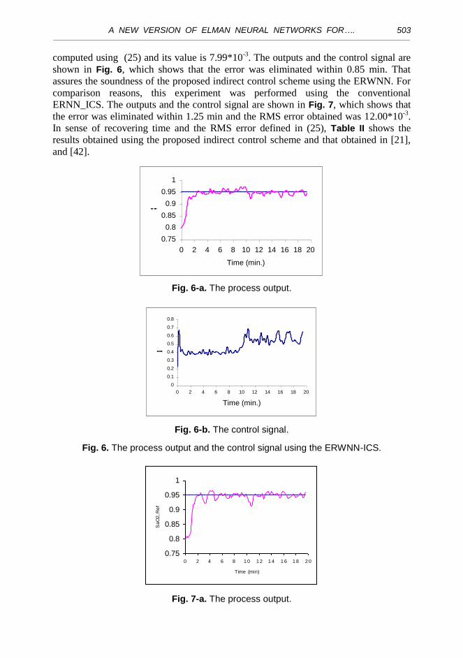
computed using (25) and its value is 7.99*10-3

. The outputs and the control signal are

shown in Fig. 6, which shows that the error was eliminated within 0.85 min. That

assures the soundness of the proposed indirect control scheme using the ERWNN. For

comparison reasons, this experiment was performed using the conventional

ERNN_ICS. The outputs and the control signal are shown in Fig. 7, which shows that

the error was eliminated within 1.25 min and the RMS error obtained was 12.00*10-3

.

In sense of recovering time and the RMS error defined in (25), Table II shows the

results obtained using the proposed indirect control scheme and that obtained in [21],

and [42].

0.75

0.8

0.85

0.9

0.95

1

0 2 4 6 8 10 12 14 16 18 20

Time (min.)

SaO

2, R

ef

Fig. 6-a. The process output.

0

0.1

0.2

0.3

0.4

0.5

0.6

0.7

0.8

0 2 4 6 8 10 12 14 16 18 20

Time (min.)

FiO

2

Fig. 6-b. The control signal.

Fig. 6. The process output and the control signal using the ERWNN-ICS.

0.75

0.8

0.85

0.9

0.95

1

0 2 4 6 8 1 0 1 2 1 4 1 6 1 8 2 0

Time (min)

Sa

O2

, Re

f

Fig. 7-a. The process output.

Hamdi A. Awad ________________________________________________________________________________________________________________________________

504

0

0.2

0.4

0.6

0.8

1

0 2 4 6 8 1 0 1 2 1 4 1 6 1 8 2 0

Time (min)

FiO

2

Fig. 7-b. The control signal.

Fig. 7. The process output and the control signal using the ERNN-ICS.

Table 2: Comparison with results published in [21] and [42].

Controller type Time required (min.) Disturbance rejection (RMS) errors

PI At least 10.00 20.50*10-3

MMAC 3.00 11.00*10-3

FNN-ICS 2.5 8.59*10-3

ERNN-ICS 1.25 12.00*10-3

ERWNN-ICS 0.85 7.99*10-3

As a final conclusion, Table 2 depicts that best results have been achieved using the

ERWNN-ICS compared with the conventional PI-controller, MMAC controller [21],

the FNN-ICS and the ERNN-ICS, [42] for controlling the O2 uptake system. In the

sense of RMS errors and time required to reject the disturbances shown in the table, the

ERWN-ICS is promising scheme for controlling real time intensive processes in noisy

conditions and disturbances. The application areas for the introduced technology are

very wide, however, the author can conclude the major application of this technology

as follows:

A universal tool for function approximation

Real time learning of unknown functions

Modelling and control time intensive real time processes

Data compression

Financial and economic analysis

Biomedical engineering

7. CONCOLUSIONS

This paper introduced a new version of Elman networks named ERWNN. Compared

with the traditional ERNN, the proposed ERWNN has three notable features, local

accuracy, generalization capability, stability and convergence property. The former

two features are inherited from replacing the global property of sigmoid functions


505

used at the hidden layer of ERNN by the multiresolution property of wavelets while the

latter is gained from employing few context/hidden units, which memorizes the

previous actions of the hidden units and can be considered to function one-step time

delay. This paper developed a model reference control scheme that belongs to indirect

adaptive control. The scheme consists of two ERWNNs, one performs the controller

and the other stands for the system’s model. This paper also derived the plant

sensitivity and DBP algorithm. The former is employed for adjusting the parameters of

the developed controller and the latter is used to train both the two networks of the

proposed indirect control scheme, ERWNN-ICS. Structurally, the number of

hidden/context units (should at least be equal to the order of the system be modeled ) of

an ERWNN employed was fixed to be six to control the actual processes with ease.

The control of the oxygen delivery to mechanically ventilated hypoxic patients is best

achieved using the proposed indirect control scheme, ERWNN-ICS, compared with the

conventional PI-controller, MMAC-controller , FNN-ICS, and ERNN-ICS.

REFERENCES

[1] K. S. Narendra and K. Parthasarathy, “Identification and control of dynamical

systems using neural networks,” IEEE Transactions on Neural Networks, vol. 1,

pp. 4-27, 1990.

[2] K. J. Hunt, D. Sbarbaro, R. Zbikowski and P. J. Gawthrop, “Neural networks for

control systems-A survey,” Automatica, vol. 28, pp. 1083-1112, 1992.

[3] G. G. Lendaris and T. T. Shannon, “Application considerations for the DHP

methodology,” Proceedings of International Joint Conference on Neural

Networks-98, (IJCNN-98), Anchorage, IEEE press, pp. 1013-1018, 1998.

[4] H. A. Awad, Fuzzy neural networks for modeling and controlling dynamic

systems. PhD. Thesis, Intelligent Systems Laboratory, School of Engineering,

Cardiff University, Cardiff, UK, 2001.

[5] D. E. Rumelhart and J. L., McClelland. Parallel distributed processing:

Explorations in the micro-structure of cognition, vol. 1, Cambridge, Mass: MIT

Press, 1986.

[6] J. L. Elman, “Finding structure in time,” Cognitive Science, vol. 14, pp. 179-211,

1990.

[7] T. Kohonen, .Self-organised and associative memory. Springer Verlag: Berlin,

1989.

[8] G. A. Carpenter, S. Grossberg and D. B. Rosen, “Fuzzy ART: Fast stable

learning and categorization of analogue patterns by an adaptive resonance

system,” Neural Networks, vol. 4, pp. 759-771, 1991.

[9] G. G. Lendaris and C. Paintz, “Training strategies for critic and action neural

networks in Dual Heuristic programming method,” Proceedings of International

Joint Conference on Neural Networks-97, (IJCNN-97), Houston, pp. 712-717,

1997.

[10] D. T. Pham and X. Liu, “Dynamic systems modeling using recurrent neural

networks,” Journal of Systems Eng., vol. 2, pp. 90-97, 1992.

[11] J. Hertz, A. Krogh and R. G. Palmer, Recurrent neural networks: Introduction to

the theory of neural computations. California: Addison-Wesley, chapter 7, 1991.

Hamdi A. Awad ________________________________________________________________________________________________________________________________

506

[12] C.-M. Kuan, Estimation of neural models. Ph.D. Thesis, University of California,

San Diego, 1989.

[13] D. T. Pham and H. X. Liu, “Training of Elman networks and dynamic system

modeling,” International Journal of syst. Sci., vol. 27, no., 2, pp. 221-226, 1996.

[14] N. M. El-Rabaie, H. A. Awad and T. A. Mahmoud, “Wavelet fuzzy neural

network-based predictive control system, ”IEEE MELECON, Dubrovnik, Croatia,

pp. 307-310, 2004.

[15] D. W. C. Ho, P.-A. Zhang and J. Xu, “Fuzzy wavelet networks for function

learning,” IEEE Transactions on Fuzzy Systems, vol. 9, pp. 200-211, 2001.

[16] C.-H. Lee and C.-C. Teng, “Identification and control of dynamic systems using

recurrent fuzzy neural networks,” IEEE Transactions on Fuzzy Systems, vol. 8,

pp. 349-366, 2000.

[17] H. Wersing, W. J. Beyn and H. Ritter, “Dynamical stability conditions for

recurrent neural networks with understanding piecewise linear transfer functions,”

Neural Computing, vol. 13, pp. 1811-1825, 2001.

[18] Y. Mitamura, T. Mikami, H. Sugawara and C. Yoshimoto, “An optimally

controlled respirator,” IEEE Trans. on Biomed Eng., vol. BME-18, pp. 330-337,

1971.

[19] Y. Sun, I. Kohane and A. Stark, “Fuzzy logic assisted control of inspired oxygen

in ventilated newborn infants,” Proc. Annu. Symp. Comput. Appl. Med. Care, pp.

756-761, 1994.

[20] Y. Sun, I. Kohane and A., Stark, “Computer-assisted adjustment of inspired

oxygen concentration improves control of oxygen saturation in newborn infants

requiring mechanical ventilation,” Journal of pediatrics, vol. 131, pp. 754-756,

1997.

[21] C. Yu and I. He, “Improvement in arterial oxygen control using multiple-model

adaptive control procedures,” IEEE Trans. Biomed Eng., vol. BME-34, p. 567,

1986.

[22] N. M. El-Rabaie, H. A. Awad, and K. T. Abo-Alam, “Arterial oxygen control

using the enhanced fuzzy neural scheme,” Al Azher University Engineerin

Journal, AUEJ, Cairo, Egypt, 2003.

[23] I. Daubechies, “Wavelet transform, time-frequency localization and signal

analysis,” IEEE Transactions on Information Theory, vol 36, pp. 961-1005, 1990.

[24] Q. Zhang, “Using wavelet networks in nonparametric estimation,” IEEE

Transactions on Neural networks, vol. 8, pp. 277-236, 1997.

[25] O. Yacine and D. Gerard, “Initialization by selection for wavelet training,”

Neural Computing, vol. 34, pp. 131-143, 2000.

[26] K. C. Kan and K. W. Wong, “Self-constriction algorithm for synthesis of wavelet

networks,” Electronic Letter, vol. 34, pp. 1953-1955, 1998.

[27] S. Chen and S. a. Billings. Neural networks for modeling and identification:

Advances in intelligent control, Edited by C. J. Harris, London, pp. 101-102,

1994.

[28] D. T. Pham and X. Liu, “Identification of linear and nonlinear dynamic systems

using recurrent neural networks,” Artificial Intelligence in Engineering, vol. 8, pp.

67-75, 1993.

[29] S. McLoone and G. Irwin, “Non-linear optimization of RBF networks,”

International Journal of Systems Science, vol. 29, pp. 179-189, 1998.


507

[30] D. R. Hush and B. G. Horne, “Progress in supervised neural networks,” IEEE

Signal Processing Magazine, pp. 8-39, 1993.

[31] G.A. Carpenter and S. Grossberg, “ART2: Self-organization of stable category

recognition codes for analogue input patterns,” Applied Optics, vol. 26, pp. 4919-

4930, 1987.

[32] H. Qiao, J. P. Jigen Z.-B. Xu and B. Zhang, “A reference model approach to

stability analysis of neural networks,” IEEE Transactions on Systems, MAN, and

Cybernetics -PARTB: Cybernetics, vol. 33, pp. 925-936, 2003.

[33] F. J. Pineda, “Generalization of back-propagation to recurrent neural networks,”

Phys. Rev. Lett., vol. 59, pp. 2229-2232, 1987.

[34] R. Rohwer and B. Forrest, “Training time-dependence in neural networks,”In

Proc. 1st IEEE Int. Conference, Neural Networks, vol. 2, San Diego, CA, pp. 701-

708, 1987.

[35] C. Yu, An arterial oxygen saturation controller, Master's thesis, , Rensselaer

Polytech. Inst., Tory, NY, 1986.

[36] J. W. Severinghaus, “Simple, accurate equations for human blood O2 dissociation

computation,” J. Appl. Phys. : Resp. Environ. Exercise Physiol., vol. 46, pp. 559-

602, 1979.

[37] C.G. Moore, Indirect adaptive fuzzy controllers. PhD. Thesis, Dept. of

Aeronautics and Astronautics, University of South Hampton, UK, 1991.

[38] K. Astrom and B. Wittenmark, Adaptive control. Reading, MA: Addison-Wesley

Pub. Co., 1989.

[39] C.-F. Juang and C.-T. Lin “A recurrent self-organizing neural fuzzy inference

network,” Proceedings of the sixth IEEE International Conference on Fuzzy

Systems, vol. III, Barcelona, Spain, 1997.

[40] A. Tsakonas and G. Dounias, “Intelligent applications- Hybrid computational

intelligence schemes in complex domains: An extended review,” In Lecture Notes

in Computer Science 2002, vol. 2308, pp. 494-512, Springer, 2002.

[41] Y.-C. Chen and C.-C. Teng, “A model reference control structure using a fuzzy

neural network,” Fuzzy sets and Systems, vol. 73, pp. 291-312, 1995.

[42] K. T. Abo Alam, Fuzzy neural control for hypoxemia. Faculty of Electronic Eng.,

Menoufia Unv., Egypt, 2005.

THE APPENDIX

In (20) assume that,

1

1,

,,

,,)(

))((*))((

n

jll

ji

jiji

lilik

kvkv

v

hh . That equation becomes,

)()1(

)(

,

kxk

k c

jx

ji

i

w

x

. Further, )1(

)(1)(

,

k

kkx

w

xx

ji

ic

j

. At time instant (k-1), It becomes:

)2(

)1(1)1(

,

k

kkx

w

xx

ji

ic

j

. Substituting this equation into (12), results:

)2(

)1(1)1(

)1(

)(1

,

,

,

k

kkxa

k

k

w

x

w

xx

ji

i

jjix

ji

i

Multiplying the resulted equation by , results:

Hamdi A. Awad ________________________________________________________________________________________________________________________________

508

)2(

)1(*)1(*)(*

)(

))((*))((

)1(

)(

,

,

1

1,

,,

,,

,

k

kkk

k

kvkv

k

k

w

xxa

v

hh

w

xx

ji

i

iji

n

lji

jiji

lilix

ji

i . the

resulted equation is equivalent to (21).

The responses of the oxygen uptake system are corrupted with additive white

Gaussian noise generated using the following algorithm [35]:

SN=RAN

SN=2.4*(SN-0.5)

SAO2=SAO2+SN/100

كيةيالنظم الدينام فينوع جديد من شبكات المان للنمذجة والتحكم

يف يتستخدم بشكل اساس يمن الشبكات العصبية ذات التغذية الراجعة والت ELMANتعتبر شبكة أن هيكلها يحتوى على يهذا النوع من الشبكات تكمن ف يف األساسيةن المشكلة إتقريب الدوال.

ذا تغيرت ظروف تشغيل العملية تتراجع إخذ حرف السيى. وهذا يعنى أنه تأ يمجموعة من الدوال التتسمى ELMANخاصية تقريب الدوال للشبكة من هذا النوع. يقدم هذا البحث نوع جديد من شبكات

ERWNN حيث يدمج هذا البحث خاصية ال .Multi-resolution لدوال المويجة مع قدرات التعلمض تحسين أدائها وتجنب مساوئ استخدام التقنتين كل على حدة. كما تم بغر ERNNصيلة ألللشبكة ا

هذا البحث. يبنى هذا البحث أيضا نظام تحكم يعتمد على الشبكة يف اختبار اتزان الشبكة المقترحةنظام التحكم المقترح. كما أشتق هذا يلتعليم شبكت DBPالمقترحة. كما تم اشتقاق و توظيف خوارزم

ييعتبر من أهم المتغيرات لضبط عناصر الحاكم المستخدم ف يوالت The plant sensitivityالبحث قترحة وكذلك نظام التحكم المعتمد عليها.مالتحكم المقترح. سوف تعكس النتائج مميزات الشبكة ال

تى:آلهذا البحث كا إسهاماتيمكن تلخيص ERWNNيسمى ERNNبناء نوع جديد من شبكات

الشبكة المقترحة لتعليم DBP اشتقاق خوارزم

اختبار اتزان الشبكة المقترحةبمجموعة من أدائهومقارنة ERWNN-ICSنظام تحكم جديد معتمدا على الشبكة المقترحة يسمى بناء

الحاكمات المماثلةيعتبر من أهم المتغيرات لضبط عناصر الحاكم المستخدم يوالت The plant sensitivityاشتقاق

نظام التحكم المقترح في Dr. Hamdy A. Awad was born in Egypt, 1964. He received the B.Sc. degree in Industrial

Electronics, and the M. Sc. degree in Adaptive Control Systems from Faculty of Electronic

Engineering, Menouf, Menoufia University, Egypt in 1988 and 1994

respectively. He received the Ph.D. degree in Artificial Intelligent

Systems in 2001 from School of Engineering, Cardiff University,

Cardiff-Wales, England. Since July 2001.

He has been with the Faculty of Electronic Engineering, Menoufia

University, where he is currently a lecturer of Control Engineering in

Industrial Electronics Engineering and Control Dept.

Dr. Awad interests in intelligent control systems, machine

learning, and their applications in control systems, fault diagnosis and

medical engineering.

a new version of elman neural networks for dynamic systems ... · a new version of elman neural...

Documents