A New Smooth Approximation to the Zero OneLoss with a Probabilistic Interpretation

Md Kamrul Hasan, Christopher J. PalDepartement de genie informatique et genie logiciel

Ecole Polytechnique MontrealMontreal, Quebec, Canada, H3T 1J4

md-kamrul.hasan@polymtl.ca, christopher.pal@polymtl.ca

Abstract

We examine a new form of smooth approximation to the zero one loss in whichlearning is performed using a reformulation of the widely used logistic function.Our approach is based on using the posterior mean of a novel generalized Beta-Bernoulli formulation. This leads to a generalized logistic function that approxi-mates the zero one loss, but retains a probabilistic formulation conferring a numberof useful properties. The approach is easily generalized to kernel logistic regres-sion and easily integrated into methods for structured prediction. We present ex-periments in which we learn such models using an optimization method consistingof a combination of gradient descent and coordinate descent using localized gridsearch so as to escape from local minima. Our experiments indicate that optimiza-tion quality is improved when learning meta-parameters are themselves optimizedusing a validation set. Our experiments show improved performance relative towidely used logistic and hinge loss methods on a wide variety of problems rangingfrom standard UC Irvine and libSVM evaluation datasets to product review pre-dictions and a visual information extraction task. We observe that the approach:1) is more robust to outliers compared to the logistic and hinge losses; 2) out-performs comparable logistic and max margin models on larger scale benchmarkproblems; 3) when combined with Gaussian- Laplacian mixture prior on parame-ters the kernelized version of our formulation yields sparser solutions than SupportVector Machine classifiers; and 4) when integrated into a probabilistic structuredprediction technique our approach provides more accurate probabilities yieldingimproved inference and increasing information extraction performance.

1 IntroductionLoss function minimization is a standard way of solving many important learning prob-lems. In the classical statistical literature, this is known as Empirical Risk Minimization(ERM) [18], where learning is performed by minimizing the average risk or loss over

1

arX

iv:1

511.

0564

3v1

[cs

.CV

] 1

8 N

ov 2

015

−4 −3 −2 −1 0 1 2 3 40

0.5

1

1.5

2

2.5

3

3.5

4

4.5

5

zi

L(z i)

Llog(zi)Lhinge(zi)L01(zi)

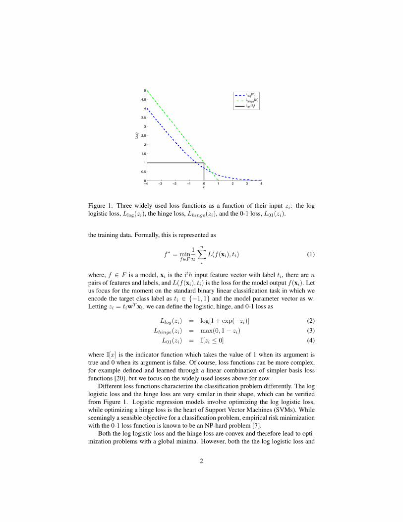
Figure 1: Three widely used loss functions as a function of their input zi: the loglogistic loss, Llog(zi), the hinge loss, Lhinge(zi), and the 0-1 loss, L01(zi).

the training data. Formally, this is represented as

f∗ = minf∈F

1

n

n∑i

L(f(xi), ti) (1)

where, f ∈ F is a model, xi is the ith input feature vector with label ti, there are npairs of features and labels, and L(f(xi), ti) is the loss for the model output f(xi). Letus focus for the moment on the standard binary linear classification task in which weencode the target class label as ti ∈ {−1, 1} and the model parameter vector as w.Letting zi = tiw

Txi, we can define the logistic, hinge, and 0-1 loss as

Llog(zi) = log[1 + exp(−zi)] (2)Lhinge(zi) = max(0, 1− zi) (3)L01(zi) = I[zi ≤ 0] (4)

where I[x] is the indicator function which takes the value of 1 when its argument istrue and 0 when its argument is false. Of course, loss functions can be more complex,for example defined and learned through a linear combination of simpler basis lossfunctions [20], but we focus on the widely used losses above for now.

Different loss functions characterize the classification problem differently. The loglogistic loss and the hinge loss are very similar in their shape, which can be verifiedfrom Figure 1. Logistic regression models involve optimizing the log logistic loss,while optimizing a hinge loss is the heart of Support Vector Machines (SVMs). Whileseemingly a sensible objective for a classification problem, empirical risk minimizationwith the 0-1 loss function is known to be an NP-hard problem [7].

Both the log logistic loss and the hinge loss are convex and therefore lead to opti-mization problems with a global minima. However, both the the log logistic loss and

2

hinge loss penalize a model heavily when data points are classified incorrectly and arefar away from the decision boundary. As can be seen in Figure 1 their penalties can bemuch more significant than the zero one loss. The zero-one loss captures the intuitivegoal of simply minimizing classification errors and recent research has been directedto learning models using a smoothed zero-one loss approximation [24, 14]. Previouswork has shown that both the hinge loss [24] and more recently the 0-1 loss [14] can beefficiently and effectively optimized directly using smooth approximations. The workin [14] also underscored the robustness advantages of the 0-1 loss to outliers. While the0-1 loss is not convex, the current flurry of activity in the area of deep neural networksas well as the award winning work on 0-1 loss approximations in [2] have highlightednumerous other advantages to the use of non-convex loss functions. In our work here,we are interested in constructing a probabilistically formulated smooth approximationto the 0-1 loss.

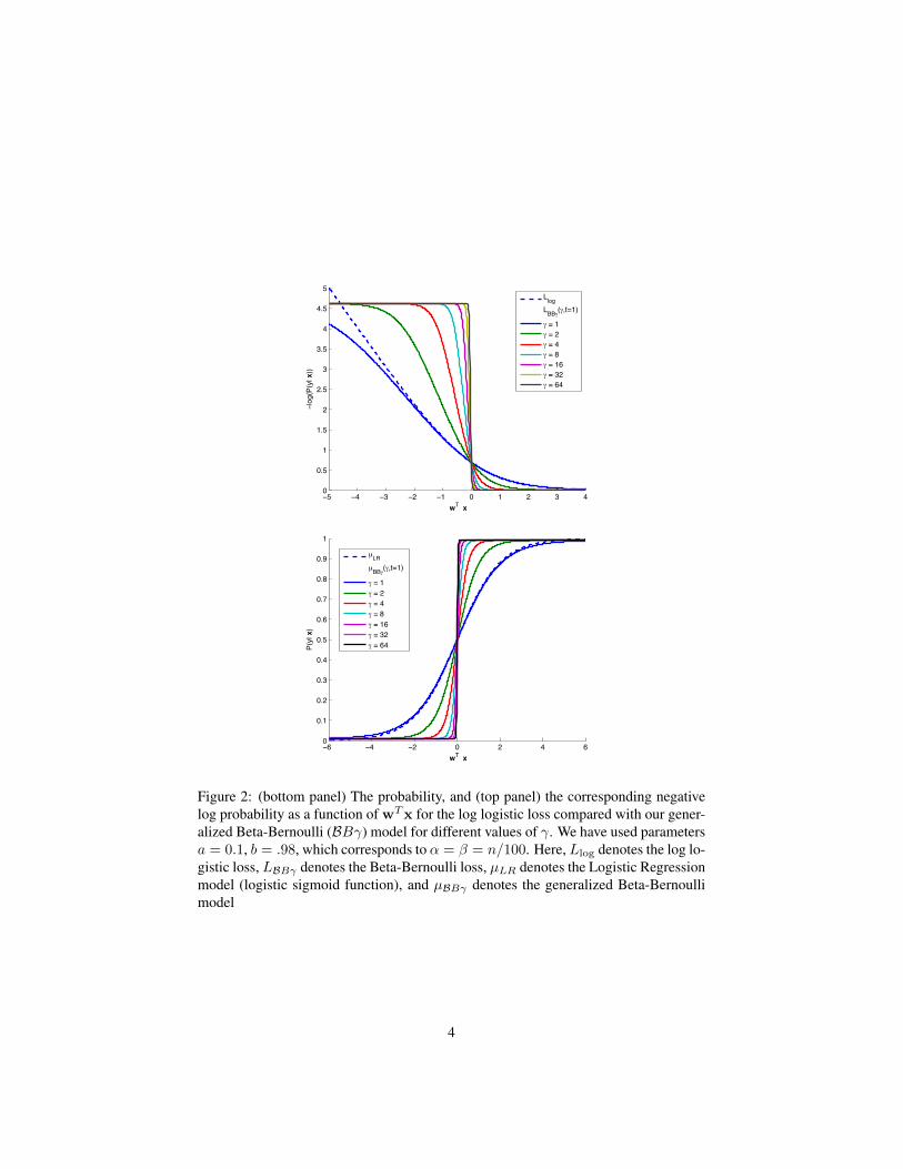
Let us first compare the widely used log logistic loss with the hinge loss and the 0-1loss in a little more detail. The log logistic loss from the well known logistic regressionmodel arises from the form of negative log likelihood defined by the model. Morespecifically, this logistic loss arises from a sigmoid function parametrizing probabilitiesand is easily recovered by re-arranging (2) to obtain a probability model of the formπ(zi) = (1 + exp(−zi))−1. In our work here, we will take this familiar logisticfunction and we shall transform it to create a new functional form. The sequence ofcurves starting with the blue curve in Figure 2 (top) give an intuitive visualization of theway in which we alter the traditional log logistic loss. We call our new loss function thegeneralized Beta-Bernoulli logistic loss and use the acronym BBγ when referring to it.We give it this name as it arises from the combined use of a Beta-Bernoulli distributionand a generalized logistic parametrization.

We give the Bayesian motivations for our Beta-Bernoulli construction in section 3.To gain some additional intuitions about the effect of our construction from a practicalperspective, consider the following analysis. When viewing the negative log likelihoodof the traditional logistic regression parametrization as a loss function, one might posethe following question: (1) what alternative functional form for the underlying prob-ability π(zi) would lead to a loss function exhibiting a plateau similar to the 0-1 lossfor incorrectly classified examples? One might also pose a second question: (2) is itpossible to construct a simple parametrization in which a single parameter controls thesharpness of the smooth approximation to the 0-1 loss? The intuition for an answer tothe first question is that the traditional logistic parametrization converges to zero proba-bility for small values of its argument. This in turn leads to a loss function that increaseswith a linear behaviour for small values of zi as shown in Figure 1. In contrast, ournew loss function is defined in such a way that for small values of zi, the function willconverge to a non-zero probability. This effect manifests itself as the desired plateau,which can be seen clearly in the loss functions defined by our model in Figure 2 (top).The answer to our second question is indeed yes; and more specifically, to control thesharpness of our approximation, we use a γ factor reminiscent of a technique used inprevious work which has created smooth approximations to the hinge loss [24] as wellas smooth approximations of the 0-1 loss [14]. We show the intuitive effect of ourconstruction for different increasing values of gamma in Figure 2 and define it moreformally below.

3

−5 −4 −3 −2 −1 0 1 2 3 40

0.5

1

1.5

2

2.5

3

3.5

4

4.5

5

wT x

−log

(P(y

| x))

LlogLBB!(!,t=1)

! = 1! = 2! = 4! = 8! = 16! = 32! = 64

−6 −4 −2 0 2 4 60

0.1

0.2

0.3

0.4

0.5

0.6

0.7

0.8

0.9

1

wT x

P(y|

x)

µLRµBB!(!,t=1)

! = 1! = 2! = 4! = 8! = 16! = 32! = 64

Figure 2: (bottom panel) The probability, and (top panel) the corresponding negativelog probability as a function of wTx for the log logistic loss compared with our gener-alized Beta-Bernoulli (BBγ) model for different values of γ. We have used parametersa = 0.1, b = .98, which corresponds to α = β = n/100. Here, Llog denotes the log lo-gistic loss, LBBγ denotes the Beta-Bernoulli loss, µLR denotes the Logistic Regressionmodel (logistic sigmoid function), and µBBγ denotes the generalized Beta-Bernoullimodel

4

To compare and contrast our loss function with other common loss functions suchas those in equations (2-4) and others reviewed below, we express our loss here usingzi and γ as arguments. For t = 1, the BBγ loss can be expressed as

LBBγ(zi, γ) = − log(a+ b[1 + exp(−γzi)]−1

), (5)

while for t = −1 it can be expressed as

LBBγ(zi, γ) = − log[1−

(a+ b[1 + exp(γzi)]

−1)]. (6)

We show in section 3 that the constants a and b have well defined interpretations interms of the standard α, β, and n parameters of the Beta distribution. Their impacton our proposed generalized Beta-Bernoulli loss arise from applying a fuller Bayesiananalysis to the formulation of a logistic function.

The visualization of our proposed BBγ loss in Figure 2 corresponds to the use ofa weak non-informative prior such as α = 1 and β = 1 and n = 100. In Figure 2,we show the probability given by the model as a function of wTx at the right and thenegative log probability or the loss on the left as γ is varied over the integer powers inthe interval [0, 10]. We see that the logistic function transition becomes more abrupt asγ increases. The loss function behaves like the usual logistic loss for γ close to 1, butprovides an increasingly more accurate smooth approximation to the zero one loss withlarger values of γ. Intuitively, the location of the plateau of the smooth log logistic lossapproximation on the y-axis is controlled by our choice of α, β and n. The effect ofthe weak uniform prior is to add a small minimum probability to the model, which canbe imperceptible in terms of the impact on the sigmoid function log space, but leads tothe plateau in the negative log loss function. By contrast, the use of a strong prior forthe losses in Figure 5 (left) leads to minimum and maximum probabilities that can bemuch further from zero and one.

Our work makes a number of contributions which we enumerate here: (1) The pri-mary contribution of our work is a new probabilistically formulated approximation tothe 0-1 loss based on a generalized logistic function and the use of the Beta-Bernoullidistribution. The result is a generalized sigmoid function in both probability and nega-tive log probability space. (2) A second key contribution of our work is that we presentand explore an adapted version of the optimization algorithm proposed in [14] in whichwe optimize the meta parameters of learning using validation sets. We present a seriesof experiments in which we optimize the BBγ loss using the basic algorithm from[14] and our modified version. For linear models, we show that our complete approachoutperforms the widely used techniques of logistic regression and linear support vectormachines. As expected, our experiments indicate that the relative performance of theapproach further increases when noisy outliers are present in the data. (3) We go onto present a number of experiments with larger scale data sets demonstrating that ourmethod also outperforms widely used logistic regression and SVM techniques despitethe fact that the underlying models involved are linear. (4) We apply our model in astructured prediction task formulated for mining faces in Wikipedia biography pages.Our proposed method is well adapted to this setting and we and find that the improvedprobabilistic modeling capabilities of our approach yields improved results for visualinformation extraction through improved probabilistic structured prediction. (5) We

5

also show how this approach is also easily adapted to create a novel form of kernel lo-gistic regression based on our generalized Beta-Bernoulli Logistic Regression (BBLR)framework. We find that the kernelized version of our method, Kernel BBLR (KBBLR)outperforms non-linear support vector machines. As expected, the L2 regularized KB-BLR does not yield sparse solutions; however, (6) since we have developed a robustmethod for optimizing a non-convex loss we propose and explore a novel non-convexsparsity encouraging prior based on a mixture of a Gaussian and a Laplacian. SparseKBBLR typically yields sparser solutions than SVMs with comparable prediction per-formance, and the degree of sparsity scales much more favorably compared to SVMs.

The remainder of this paper is structured as follows. In section 2, we present areview of some relevant recent work in the area of 0-1 loss approximation. In section3, we present the underlying Bayesian motivations for our proposed loss function. Insection 4, we provide with the details of optimization and algorithms. In section 5,we present experimental results using protocols that both facilitate comparisons withprior work as well as evaluate our method on some large scale and structured predictionproblems. We provide a final discussion and conclusions in section 6.

2 Relevant Recent WorkIt has been shown in [24] that it is possible to define a generalized logistic loss andproduce a smooth approximation to the hinge loss using the following formulation

Lglog(ti,xi;w, γ) =1

γlog[1 + exp(γ(1− tiwTxi))], (7)

Lglog(zi, γ) = γ−1 log[1 + exp(γ(1− zi))], (8)

such that limγ→∞ Lglog = Lhinge. We have achieved this approximation using a γfactor and a shifted version of the usual logistic loss. We illustrate the way in whichthis construction can be used to approximate the hinge loss in Figure 3 (left).

The maximum margin Bayesian network formulation in [16] also employs a smoothdifferentiable hinge loss inspired by the Huber loss, having a similar shape tomin[1, zi].The sparse probabilistic classifier approach in [10] truncates the logistic loss leadingto a sparse kernel logistic regression models. [15] proposed a technique for learningsupport vector classifiers based on arbitrary loss functions composed of using the com-bination of a hyperbolic tangent loss function and a polynomial loss function.

Other recent work [14] has created a smooth approximation to the 0-1 loss by di-rectly defining the loss as a modified sigmoid. They used the following function

Lsig(ti,xi;w, γ) =1

1 + exp(γtiwTxi), (9)

Lsig(zi, γ) = [1 + exp(γzi)]−1. (10)

In a way similar to the smooth approximation to the hinge loss, here limγ→∞ Lsig =L01. We illustrate the way in which this construction approximates the 0-1 loss inFigure 3 (right).

6

−3 −2 −1 0 1 2 30

0.5

1

1.5

2

2.5

3

3.5

4

4.5

zi

L(z i)

Llog(zi)Llog(zi−1)Lglog(zi,!=2)Lglog(zi,!=4)

Lhinge(zi)

−2 −1.5 −1 −0.5 0 0.5 1 1.5 20

0.1

0.2

0.3

0.4

0.5

0.6

0.7

0.8

0.9

1

zi

L(z i)

Lhinge(zi)Lsig(zi,!=1)

Lsig(zi,!=2)

Lsig(zi,!=32)

Figure 3: (left) The way in which the generalized log logistic loss, Lglog proposed in[24] can approximate the hinge loss, Lhinge through translating the log logistic loss,Llog then increasing the γ factor. We show here the curves for γ = 2 and γ = 4.(right) The way in a sigmoid function is used in [14] to directly approximate the 0-1loss, L01. The approach also uses a similar γ factor to [24] and we show γ = 1, 2 and32.

Another important aspect of [14] is that they compared a variety of algorithms fordirectly optimizing the 0-1 loss with a novel algorithm for optimizing the sigmoid loss,Lsig(zi, γ). They call their algorithm Smooth 0–1 Loss Approximation (SLA) forsmooth loss approximation. The compared direct 0-1 loss optimization algorithms are:(1) a Branch and Bound (BnB) [11] technique, (2) a Prioritized Combinatorial Search(PCS) technique and (3) an algorithm referred to as a Combinatorial Search Approxi-mation (CSA), both of which are presented in more detail in [14]. They compared thesemethods with the use of their SLA algorithm to optimize the sigmoidal approximationto the 0-1 loss.

To evaluate and compare the quality of the non-convex optimization results pro-duced by the BnB, PCS and CSA, with their SLA algorithm for the sigmoid loss, [14]also presents training set errors for a number of standard evaluation datasets. We pro-vide an excerpt of their results in Table 1 as we will perform similar comparisons inour experimental work. These results indicated that the SLA algorithm consistentlyyielded superior performance at finding a good minima to the underlying non-convexproblem. Furthermore, in [14], they also provide an analysis of the run-time perfor-mance for each of the algorithms. Their experiments indicated that the SLA techniquewas significantly faster than the alternative algorithms for non-convex optimization.Based on these results we build upon the SLA approach in our work here.

The award winning work of [2] produced an approximation to the 0-1 loss by creat-ing a ramp loss, Lramp, obtained by combining the traditional hinge loss with a shiftedand inverted hinge loss as illustrated in Figure 4. They showed how to optimize theramp loss using the Concave-Convex Procedure (CCCP) of [23] and that this yieldsfaster training times compared to traditional SVMs. Other more recent work has pro-posed an alternative online SVM learning algorithm for the ramp loss [6]. [22] explored

7

Table 1: An excerpt from [14] of the total 0-1 loss for a variety of algorithms on somestandard datasets. The 0-1 loss for logistic regression (LR) and a linear support vectormachine (SVM) are also provided for reference.

LR SVM PCS CSA BnB SLABreast 19 18 19 13 10 13Heart 39 39 33 31 25 27Liver 99 99 91 91 95 89Pima 166 166 159 157 161 156Sum 323 322 302 292 291 285

a similar ramp loss which they refer to as a robust truncated hinge loss. More recentwork [3] has explored a similar ramp like construction which they refer to as the slantloss. Interestingly, the ramp loss formulation has also been generalized to structuredpredictions [4, 8].

−3 −2 −1 0 1 2 3−3

−2

−1

0

1

2

3

4

zi

L(z i)

Lhinge(zi,s=1)

−3 −2 −1 0 1 2 3−3

−2

−1

0

1

2

3

4

zi

L(z i)

−Lhinge(zi,s=−1)

−3 −2 −1 0 1 2 3−3

−2

−1

0

1

2

3

4

zi

L(z i)

Lramp(zi,s=1)

Figure 4: The way in which shifted hinge losses are combined in [2] to produce theramp loss, Lramp. The usual hinge loss (left), Lhinge is combined with the negative,shifted hinge loss, Lhinge(zi, s = −1) (middle), to produce Lramp (right).

Although the smoothed zero-one loss captured much attention recently, we can findolder references to similar research. There has been the activity of using zero-one losslike functional losses in machine learning, specially by the boosting [13] and neuralnetwork [19] communities. Vincent [19] analyzes that the loss defined through a func-tional of the hyperbolic tangent, 1− tanh(zi), is more robust as it doesn’t penalize theoutliers too excessively compared to other { log logistic loss, hinge loss, and squaredloss } loss functions. This loss has interesting properties of both being continuous andwith zero-one loss like properties. A variant of this loss has been used in boosting al-gorithms [13]. Other work [19] has also shown that a hyperbolic tangent parametrizedsquared error loss, (0.65 − tanh(zi))

2, transforms the squared error loss to behavemore like the 1− tanh(z), hyperbolic tangent loss.

We shall see below how it is also possible to integrate our novel smooth loss formu-lation into models for structured prediction. In this way our work is similar to that of[8] which explored the use of the ramp loss of [2] in the context of structured predictionfor machine translation.

8

3 Our Approach: Generalized Beta-Bernoulli LogisticClassification

We now derive a novel form of logistic regression based on formulating a generalizedsigmoid function arising from an underlying Bernoulli model with a Beta prior. Wealso use a γ scaling factor to increase the sharpness of our approximation. Considerfirst the traditional and widely used formulation of logistic regression which can bederived from a probabilistic model based on the Bernoulli distribution. The Bernoulliprobabilistic model has the form:

P (y|θ) = θy(1− θ)(1−y), (11)

where y ∈ {0, 1} is the class label, and θ is the parameter of the model. The Bernoullidistribution can be re-expressed in standard exponential family form as

P (y|θ) = exp{log( θ

1− θ

)y + log(1− θ)

}, (12)

where the natural parameter η is given by

η = log( θ

1− θ

)(13)

In traditional logistic regression, we let the natural parameter η = wTx, which leadsto a model where θ = θML in which the following parametrization is used

θML = µML(w,x) =1

1+ exp(−η)=

1

1+ exp(−wTx)(14)

The conjugate distribution to the Bernoulli is the Beta distribution

Beta(θ|α, β) = 1

B(α, β)θα−1(1− θ)β−1 (15)

where α and β have the intuitive interpretation as the equivalent pseudo counts for ob-servations for the two classes of the model and B(α, β) is the beta function. When weuse the Beta distribution as the prior over the parameters of the Bernoulli distribution,the posterior mean of the Beta-Bernoulli model is easily computed due to the fact thatthe posterior is also a Beta distribution. This property also leads to an intuitive formfor the posterior mean or expected value θBB in a Beta-Bernoulli model, which con-sists of a simple weighted average of the prior mean θB and the traditional maximumlikelihood estimate, θML, such that

θBB = wθB + (1− w)θML, (16)

wherew =

α+ β

α+ β + n, and θB =

( α

α+ β

),

and where n is the number of examples used to estimate θML. Consider now the taskof making a prediction using a Beta posterior and the predictive distribution. It is

9

easy to show that the mean or expected value of the posterior predictive distribution isequivalent to plugging the posterior mean parameters of the Beta distribution into theBernoulli distribution, Ber(y|θ), i.e.

p(y|D) =∫ 1

0

p(y|θ)p(θ|D)dθ = Ber(y|θBB). (17)

Given these observations, we thus propose here to replace the traditional sigmoidalfunction used in logistic regression with the function given by the posterior mean ofthe Beta-Bernoulli model such that

µBB(w,x) = w( α

α+ β

)+ (1− w)µML(w,x) (18)

Further, to increase our model’s ability to approximate the zero one loss, we shallalso use a generalized form of the Beta-Bernoulli model above where we set the naturalparameter of µML so that η = γwTx. This leads to our complete model based on ageneralized Beta-Bernoulli formulation

µBBγ(w,x) = w( α

α+ β

)+ (1− w) 1

1 + exp(−γwTx). (19)

It is useful to remind the reader at this point that we have used the Beta-Bernoulliconstruction to define our function, not to define a prior over the parameter of a randomvariable as is frequently done with the Beta distribution. Furthermore, in traditionalBayesian approaches to logistic regression, a prior is placed on the parameters w andused for MAP parameter estimation or more fully Bayesian methods in which oneintegrates over the uncertainty in the parameters.

In our formulation here, we have placed a prior on the function µML(w,x) as iscommonly done with Gaussian processes. Our approach might be seen as a pragmaticalternative to working with the fully Bayesian posterior distributions over functionsgiven data, p(f |D). The more fully Bayesian procedure would be to use the posteriorpredictive distribution to make predictions using

p(y∗|x∗,D) =∫p(y∗|f, x∗)p(f |D)df. (20)

Let us consider again the negative log logistic loss function defined by our gener-alized Beta-Bernoulli formulation where we let z = wT x and we use our y ∈ {0, 1}encoding for class labels. For y = 1 this leads to

− log p(y = 1|z) = − log

[wθβ +

(1− w)1 + exp(−γz)

], (21)

while for the case when y = 0, the negative log probability is simply

− log p(y = 0|z) = − log

(1−

[wθβ +

(1− w)1 + exp(−γz)

])(22)

10

where wθβ = a and (1 − w) = b for the formulation of the corresponding loss givenearlier in equations (5) and (6).

In Figure 2 we showed how setting this scalar parameter γ to larger values, i.e� 1allows our generalized Beta-Bernoulli model to more closely approximate the zero oneloss. We show the BBγ loss with a = 1/4 and b = 1/2 in Figure 5 (left) whichcorresponds to a stronger Beta prior and as we can see, this leads to an approximationwith a range of values that are even closer to the 0-1 loss. As one might imagine, witha little analysis of the form and asymptotics of this function, one can also see that forgiven a setting of α = β and n, a corresponding scaling factor s and linear translationc can be found so as to transform the range of the loss into the interval [0, 1] such thatlimγ→∞ s(LBBγ − c) = L01. However, when α 6= β as shown in Figure 5 (right),the loss function is asymmetric and in the limit of large gamma this corresponds todifferent losses for true positives, false positives, true negatives and false negatives.For these and other reasons we believe that this formulation has many attractive anduseful properties.

!! !" !# !$ !% & % $ # " !&'$

&'"

&'(

&')

%

%'$

%'"

%'(

w*+ x

!,-./0/12 x33

+

+

!+4+%

!+4+$

!+4+"

!+4+)

!+4+%(

!+4+#$

!+4+("

−4 −3 −2 −1 0 1 2 3 40

0.5

1

1.5

2

2.5

3

3.5

4

wT x

−log

(P(y

| x))

LlogLBB!(!=8,t=1)

LBB!(!=8,t=−1)

Figure 5: (left) The BBγ loss, or the negative log probability for t = 1 as a function ofwTx under our generalized Beta-Bernoulli model for different values of γ. We haveused parameters a = 1/4 and b = 1/2, which corresponds to α = β = n/2. (right)The BBγ loss also permits asymmetric loss functions. We show here the negative logprobability for both t = 1 and t = −1 as a function of wTx with γ = 8. This losscorresponds to α = n, β = 2n. We also give the log logistic loss as a point of reference.Here, Llog(zi) denotes the log logistic loss, and LBBγ(zi) denotes the Beta-Bernoulliloss.

3.1 Parameter Estimation and GradientsWe now turn to the problem of estimating the parameters w, given data in the formof D = {yi,xi}, i = 1, . . . , n, using our model. As we have defined a probabilisticmodel, as usual we shall simply write the probability defined by our model then opti-mize the parameters via maximizing the log probability or minimizing the negative logprobability. As we shall discuss in more detail in section 4, we use a modified form ofthe SLA optimization algorithm in which we slowly increase γ and interleave gradientdescent steps with coordinate descent implemented as a grid search. For the gradient

11

descent part of the optimization we shall need the gradients of our loss function and wetherefore give them below.

Consider first the usual formulation of the conditional probability used in logisticregression

P ({yi}|{xi},w) =

n∏i=1

µyii (1− µi)(1−yi), (23)

here in place of the usual µi, in our generalized Beta-Bernoulli formulation we nowhave µi = µβB(ηi) where ηi = γwTxi. Given a data set D consisting of label andfeature vector pairs, this yields a log-likelihood given by

L = logP (D|w) =

n∑i=1

(yi logµi + (1− yi) log(1− µi)

)(24)

where the gradient of this function is given by

dLdw

=

n∑i=1

( yiµi− 1− yi

1− µi

)dµidηi

dηidw

(25)

withdµidηi

= (1− w) exp(−ηi)(1 + exp(−ηi))2

anddηidw

= γx. (26)

3.2 Some Asymptotic AnalysisAs we have stated at the beginning of our discussion on parameter estimation, at theend of our optimization we will have a model with a large γ. With a sufficiently large γall predictions will be given their maximum or minimum probabilities possible underthe βBγ model. Defining the t = 1 class as the positive class, if we set the maximumprobability under the model equal to the True Positive Rate (TPR) (e.g. on trainingand/or validation data) and the maximum probability for the negative class equal to theTrue Negative Rate (TNR) we have

wθβ + (1− w) = TPR, (27)1− wθB = TNR, (28)

which allows us to conclude that this would equivalently correspond to setting

w = 2− (TNR+ TPR), (29)

θB =1− TNR

2− (TNR+ TPR). (30)

This analysis gives us a good idea of the expected behavior of the model if we optimizew and θB on a training set. It also suggests that an even better strategy for tuning wand θB would be to use a validation set.

12

3.3 Learning hyper-parametersWe have provided an asymptotic analysis of the expected values for w and θB in theprevious section. In the experiment section, we provide BBLR results for using asymp-totic values of these two parameters along with cross-validated values for other hyper-parameters {γ, λ}, where λ is the regularization parameter described in Section 4. It ishowever also possible to learn these hyper-parameters using the training set, validationset or both. Below, we provide partial-derivatives of likelihood function (24) for thesehyper-parameters.

dLdw

=

n∑i=1

( yiµi− 1− yi

1− µi

)dµidw

(31)

withdµidw

= θB −1

1 + exp(−γwTx)(32)

The partial-derivatives with respect to θB and γ are as follows

dLdθB

= w

n∑i=1

( yiµi− 1− yi

1− µi

)(33)

dLdγ

=

n∑i=1

( yiµi− 1− yi

1− µi

)dµidηi

dηidγ

(34)

withdµidηi

= (1− w) exp(−ηi)(1 + exp(−ηi))2

anddηidγ

= wTx. (35)

3.4 Kernel Beta-Bernoulli ClassificationIt is possible to transform the traditional logistic regression technique discussed aboveinto a kernel logistic regression (KLR) by replacing the linear discriminant function,η = wT x, with

η = f(a, x) =N∑j=1

ajK(x, xj), (36)

where K(x, xj) is a kernel function and j is used as an index in the sum over all Ntraining examples.

To create our generalized Beta-Bernoulli KLR model we take a similar path; how-ever, in this case we let η = γf(a, x). Thus, our Kernel Beta-Bernoulli model can bewritten as:

µKβB(a,x) = w( α

α+ β

)+

(1− w)1 + exp

(− γf(a,x)

) . (37)

If we write f(a, x) = aTk(x), where k(x) is a vector of kernel values, then the gradientof the corresponding KBBLR log likelihood obtained by setting µi = µKβB(a,x) in

13

(24) isdL

da= γ(1− w)

n∑i=1

k(xi)( yiµi− 1− yi

1− µi

) exp(−ηi)(1 + exp(−ηi))2

. (38)

4 Optimization and AlgorithmsAs we have discussed in the relevant recent work section above, the work of [14] hasshown that their SLA algorithm applied to Lsig(zi, γ) outperformed a number of othertechniques in terms of both true 0-1 loss minimization performance and run time. Asour generalized Beta-Bernoulli loss, LBBγ(zi, γ) is another type of smooth approxi-mation to the 0-1 loss, we therefore use a variation of their SLA algorithm to optimizethe BBγ loss. Recall that if one compares our generalized Beta-Bernoulli logistic losswith the directly defined sigmoidal loss used in the SLA work of [14], it becomes ap-parent that the BBLR formulation has three additional hyper-parameters, {α, β, w}.These additional parameters control the locations of the plateaus of our function andthese plateaus have well defined interpretations in terms of probabilities. In contrast,the plateaus of the sigmoidal loss in [14] are located at zero and one. Additionally, inpractise one is interested in optimizing the regularized loss, where some form of prioror regularization is used for parameters. In our experiments here, we follow the widelyused practice of using a Gaussian prior for parameters. The corresponding regularizedloss arising from the negative log likelihood with the additional L2 regularization termgives us our complete objective function

L(D|w) = −n∑i=1

(yi logµi + (1− yi) log(1− µi)

)+λ

2‖w‖2, (39)

where the parameter λ controls the strength of the regularization. With these additionalhyper-parameters {α, β, w, λ}, the original SLA algorithm is not directly applicable toour formulation. However, if we hold these hyper-parameters fixed, we are able to usethe general idea of their approach and perform a Modified SLA optimization as givenin Algorithms 1 and 2. In our experiments below, we use that strategy in the BBLR1,2,3

series of experiments. To deal with the issue of how to jointly learn weights w as wellas hyper-parameters w, α, β, λ and γ; in our BBLR4 series of experiments we learnthese hyper-parameters by gradient descent on the training set. More precisely, welearn w and θB (as opposed to learning α, β) as this permit the parameters to be easilyre-parametrized so that they both lie within [0, 1].

Very importantly, our initial experiments indicated that the basic SLA formula-tion required considerable hand tuning of learning parameters for each new data set.This was the case even using the simplest smooth loss function without the addi-tional degrees of freedom afforded by our formulation. This led us to develop a meta-optimization procedure for learning algorithm parameters. The BBLR3,4 series of ex-periments below use this learning meta-parameter optimization procedure. Our initialand formal experiments here indicate that this meta-optimization of learning parame-ters is in fact essential in practice. We therefore present it in more detail below.

14

4.1 Our SLA Algorithm Meta-optimization (SLAM)Here we present our meta-optimization extension and various other modifications tothe SLA approach of [14]. The SLA algorithm proposed in [14] can be decomposedinto two different parts; an outer loop that initializes a model then enters a loop inwhich one slowly increases the γ factor of their sigmoidal loss, repeatedly calling analgorithm they refer to as Range Optimization for SLA or Gradient Descent in Range.The Range Optimization part consists of two stages. Stage 1 is a standard gradientdescent optimization with a decreasing learning rate (using the new γ factor). Stage 2probes each parameter wi in a radius R using a one dimensional grid search to deter-mine if the loss can be further reduced, thus implementing a coordinate descent on a setof grid points. We provide a slightly modified form of the outer loop of their algorithmin Algorithm 1 where we have expressed the initial parameters given to the model, w0

as explicit parameters given to the algorithm. In their approach they hard code theinitial parameter estimates as the result of an SVM run on their data. We provide acompressed version of their inner Range optimization technique in Algorithm 2.

Algorithm 1 Modified SLA - Initialization and outer loopInput: Training data X, t, and initial weights w0, and

constants: R0, εS0 , γMIN , γMAX , rγ , rR, rεOutput: w∗, estimated weights minimizing 0-1 loss.

1: function FIND-SLA-SOLUTION(X,t,w0)2: w← w0

3: R← R0

4: εS ← εS0

5: γ ← γMIN

6: while γ ≤ γMAX do7: w∗ ← GRAD-DESC-IN-RANGE(w∗,X, t, γ, R, εS)8: γ ← rγγ9: R← rRR

10: εS ← rεεS11: end while12: return w∗

13: end function

The first minor difference between the SLA optimization algorithm of [14] andour extension to it are the selection of the initial w0 that the SLA algorithm startsoptimizing. While the original SLA algorithm uses the SVM solution as its initialsolution, w0, our modified SLA algorithm uses the γ and λ obtained from experimentsusing a validation set defined within the training data to initialize w0 for the gradientbased optimization technique which will start from w = 0. The idea here is to searchfor the best γ and λ that produces a reasonable solution of w that the SLA algorithmwill start with, where λ is the weight associated with the Gaussian prior leading to L2penalty added to (24).

Our meta-optimization procedure consists of the following. We use the suggestedvalues in the original SLA algorithm [14] for the parameters rR, R0, rε, and εS0

. For

15

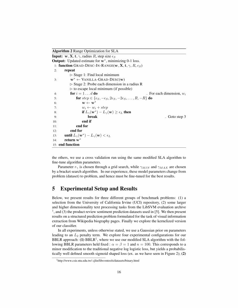
Algorithm 2 Range Optimization for SLAInput: w,X, t, γ, radius R, step size εSOutput: Updated estimate for w∗, minimizing 0-1 loss.

1: function GRAD-DESC-IN-RANGE(w,X, t, γ, R, εS)2: repeat

B Stage 1: Find local minimum3: w∗ ← VANILLA-GRAD-DESC(w)

B Stage 2: Probe each dimension in a radius RB to escape local minimum (if possible)

4: for i = 1 . . . d do . For each dimension, wi5: for step ∈ {εS ,−εS , 2εS ,−2εS , . . . , R,−R} do6: w← w∗

7: wi ← wi + step8: if Lγ(w∗)− Lγ(w) ≥ εL then9: break . Goto step 3

10: end if11: end for12: end for13: until Lγ(w∗)− Lγ(w) < εL14: return w∗

15: end function

the others, we use a cross validation run using the same modified SLA algorithm tofine-tune algorithm parameters.

Parameter rγ is chosen through a grid search, while γMIN and γMAX are chosenby a bracket search algorithm. In our experience, these model parameters change fromproblem (dataset) to problem, and hence must be fine-tuned for the best results.

5 Experimental Setup and ResultsBelow, we present results for three different groups of benchmark problems: (1) aselection from the University of California Irvine (UCI) repository, (2) some largerand higher dimensionality text processing tasks from the LibSVM evaluation archive1, and (3) the product review sentiment prediction datasets used in [5]. We then presentresults on a structured prediction problem formulated for the task of visual informationextraction from Wikipedia biography pages. Finally we explore the kernelized versionof our classifier.

In all experiments, unless otherwise stated, we use a Gaussian prior on parametersleading to an L2 penalty term. We explore four experimental configurations for ourBBLR approach: (1) BBLR1, where we use our modified SLA algorithm with the fol-lowing BBLR parameters held fixed : α = β = 1 and n = 100. This corresponds to aminor modification to the traditional negative log logistic loss, but yields a probabilis-tically well defined smooth sigmoid shaped loss (ex. as we have seen in Figure 2); (2)

1http://www.csie.ntu.edu.tw/ cjlin/libsvmtools/datasets/binary.html

16

BBLR2, where we use values for α, β and n corresponding to the empirical counts ofpositives, negatives and the total number of examples from the training set, which cor-responds to a simplistic heuristic, partially justified by Bayesian reasoning; (3) BBLR3

in which an outer meta-optimization of learning parameters is performed on top of (2),ie SLAM, and (4) BBLR4 in which the outer meta-optimization of learning parame-ters is performed, and the hyper-parameters w, θB , λ, and γ are optimized by gradientdescent using the training set, with w and θB initialized using the values given by ourasymptotic analysis using a hard threshold for classifications. At each iteration of thisoptimization step, as parameters {w, θB , λ, γ} get updated, the complementary SLAMhyper-parameters, γR, γMIN , γMAX are adjusted/redefined by using the same meta-optimization procedure (SLAM) and using a subset of the training data as a validationset.

Consequently, models produced by the BBLR3 series of experiments explore theability of our improved SLA learning parameter meta-optimization method (SLAM) toeffectively minimize a smooth approximation to the zero one loss. While the BBLR4

series of experiments delve the deepest into the ability of our BBLR formulation andSLAM optimization to more accurately make probabilistic predictions.

5.1 Binary Classification Tasks5.1.1 Experiments with UCI Benchmarks

We evaluate our technique on the following datasets from the University of CaliforniaIrvine (UCI) Machine Learning Repository [1]: Breast, Heart, Liver and Pima. We usethese datasets in part so as to compare directly with results in [14], to understand thebehaviour of our novel logistic function formulation and to explore the behavior of ourlearning parameter optimization procedure. Table 2 shows some brief details of thesedatabases.

Table 2: Standard UCI benchmark datasets used for our experiments.

Dataset # Examples # Dimensions DescriptionBreast 683 10 Breast Cancer Diagnosis [12]Heart 270 13 StatlogLiver 345 6 Liver DisordersPima 768 8 Pima Indians Diabetes

To facilitate comparisons with previous results presented [14] such as those sum-marized in Table 3 of our literature review in Section 2, we provide a small set of initialexperiments here following their experimental protocols. In our experiments here wecompare our BBLRs with the following models: our own L2 Logistic Regression (LR)implementation, a linear SVM - using the same implementation (liblinear) that wasused in [14], and the optimization of the sigmoid loss, Lsig(zi, γ) of [14] using theSLA algorithm and the code distributed on the web site associated with [14] (indicatedby SLA in our tables).

17

Despite the fact that we used the code distributed on the website associated with[14] we found that the SLA algorithm applied to their sigmoid loss, Lsig(zi, γ) gaveerrors that are slightly higher than those given in [14]. We use the term SLA in Table 3and subsequent tables to denote experiments performed using both the sigmoidal lossexplored in [14] and their algorithm for minimizing it. Applying the SLA algorithm toourBBγ loss yielded slightly superior results to the sigmoidal loss when the empiricalcounts from the training set for α, β and n are used and slightly worse results when weused α = 1, β = 1 and n = 100.

Analyzing the ability of different loss formulations and algorithms to minimize the0-1 loss on different datasets using a common model class (i.e. linear models) can re-veal differences in optimization performance across different models and algorithms.However, we are certainly more interested in evaluating the ability of different lossfunctions and optimization techniques to learn models that can be generalized to newdata. We therefore provide the next set of experiments using traditional training, val-idation and testing splits, again following the protocols used in [14]; however, as weshall soon see, these experiments underscored the importance of extending the originalSLA algorithm to automate the adjustment of learning parameters.

In Tables 4 and 5, we create 10 random splits of the data and perform a traditional 5fold evaluation using cross validation within each training set to tune hyper-parameters.In Table 4, we present the sum of the 0-1 loss over each of the 10 splits as well asthe total 0-1 loss across all experiments for each algorithm. This analysis allows usto make some intuitive comparisons with the results in Table 1, which represents anempirically derived lower bound on the 0-1 loss. In Table 5, we present the traditionalmean accuracy across these same experiments. Examining columns SLA vs. BBLR2 inTable 4, we see that our re-formulated logistic loss is able to outperform the sigmoidalloss, but that only with the addition of the additional tuning of parameters during theoptimization in column BBLR3 are we able to improve upon the overall zero-one lossyielded by the logistic regression and SVM baseline methods. However, it is importantto remember that all of these methods are based on an underlying linear model, theseare comparatively small datasets consisting of relatively low dimensional input featurevectors. As such, we do not necessarily expect there to be any statistically significantdifferences test set performance due to zero-one loss minimization performance. Thesame observation was made in [14] and it motivated their own exploration of learningwith noisy feature vectors. We follow a similar path below, but then go on further toexplore datasets that are much larger and of much higher dimensions in our subsequentexperimental work.

In Table 6, we present the sum of the mean 0-1 loss over 10 repetitions of a 5 foldleave one out experiment where 10% noise has been added to the data following theprotocol given in [14]. Here again, our BBLR2 achieved a moderate gain over the SLAalgorithm, whereas the gain of BBLR3 over other models is noticeable. In this table,we also show the percentage of improvement for our best model over the linear SVM.In Table 7, we show the average errors (%) for these 10% noise added experiments. Wesee here that the advantages of more directly approximating the zero one loss are morepronounced. However, the fact that the SLA approach failed to outperform the LR andSVM baselines in our experiments here; whereas in a similar experiment in [14] theSLA algorithm and sigmoidal loss did outperform these methods leads us to believe

18

Table 3: The total 0-1 loss for all data in a dataset. (left to right) Results using logisticregression, a linear SVM, our method with α = β = 1 and n = 100 (BBLR1), thesigmoid loss with the SLA algorithm and our approach with empirical values for α, βand n (BBLR2).

Dataset LR SVM BBLR1 SLA BBLR2

Breast 21 19 11 14 12Heart 39 40 42 39 26Liver 102 100 102 90 90Pima 167 167 169 157 166Sum 329 326 324 300 294

Table 4: The sum of the mean 0-1 loss over 10 repetitions of a 5 fold leave one outexperiment. (left to right) Performance using logistic regression, a linear SVM, thesigmoid loss with the SLA algorithm, our BBLR model with optimization using theSLA optimization algorithm and our BBLR models (BBLR2 and BBLR3) with addi-tional tuning of the modified SLA algorithm.

LR SVM SLA BBLR2 BBLR3

Breast 22 21 23 22 21Heart 45 45 48 50 43Liver 109 110 114 105 105Pima 172 172 184 176 171

Total L01 348 348 368 354 340

Table 5: The errors (%) averaged across the 10 test splits of a 5 fold leave one out exper-iment. (left to right) Performance using logistic regression, a linear SVM, the sigmoidloss with the SLA algorithm, our BBLR model with optimization using the SLA opti-mization algorithm and our BBLR model with additional tuning of the modified SLAalgorithm.

LR SVM SLA BBLR2 BBLR3 BBLR4

Breast 3.2 3.1 3.6 3.2 3.1 3.0Heart 16.8 16.6 17.7 18.6 15.9 15.7Liver 31.5 31.8 32.9 30.6 30.4 30.5Pima 22.3 22.4 23.9 23.0 22.2 22.2

that the issue of per-dataset learning algorithm parameter tuning is a significant issue.However, we observe that our BBLR2 experiment which used the original SLA opti-mization algorithm outperformed the sigmoidal loss function optimized using the SLAalgorithm. These results support the notion that our proposed Beta-Bernoulli logisticloss is in itself a superior approach to approximate the zero-one loss from an empirical

19

Table 6: The sum of the mean 0-1 loss over 10 repetitions of a 5 fold leave one outexperiment where 10% noise has been added to the data following the protocol givenin [14]. (left to right) Performance using logistic regression, a linear SVM, the sigmoidloss with the SLA algorithm, our BBLR model with optimization using the SLA opti-mization algorithm and our BBLR model with additional tuning of the modified SLAalgorithm. We give the relative improvement in error of the BBLR3 technique over theSVM in the far right column.

LR SVM SLA BBLR2 BBLR3 Impr.Breast 36 34 26 26 25 26%Heart 44 44 49 47 42 4%Liver 150 149 149 149 117 21%Pima 192 199 239 185 174 12%

Total L01 422 425 463 374 359 16%

Table 7: The errors (%) averaged over 10 repetitions of a 5 fold leave one out experi-ment in which 10% noise has been added to the data. (left to right) Performance usinglogistic regression, a linear SVM, the sigmoid loss with the SLA algorithm, our BBLRmodel with optimization using the SLA optimization algorithm and our BBLR modelwith additional tuning of the modified SLA algorithm.

LR SVM SLA BBLR2 BBLR3 BBLR4

Breast 5.2 5.0 3.8 3.9 3.7 3.4Heart 16.4 16.2 18.1 17.3 15.5 15.2Liver 43.5 43.1 43.3 33.8 34.1 34.0Pima 25.0 25.9 31.1 24.0 22.7 22.5

perspective. However, our results in column BBLR4 indicate that the combined useof our novel logistic loss and learning parameter optimization yield the most substan-tial improvements to zero-one loss minimization, or correspondingly improvements toaccuracy.

5.1.2 Pooled McNemar Tests :

We performed McNemar tests for the four UCI benchmarks comparing BBLR3 withLR and linear SVMs. As we do not have significant number of test instances for anyof these benchmarks, it became difficult to statistically justify and compare results.Therefore, we performed pooled McNemar tests by considering each split of our 5-fold leave one out experiments as independent tests and collectively performing thesignificance tests as a whole. The results of this pooled McNemar test is given inTable 8. Interestingly, for our noisy dataset experiments, our BBLR3 was found to bestatistically significant over both the LR and SVM models with p ≤ 0.01.

20

Table 8: z-static for pooled McNemar tests; values ≥ 2.32 denotes statistically signifi-cance with p ≤ 0.01.

BBLR3 vs. LR BBLR3 vs. SVMclean-UCI 3.17 0.69noisy-UCI 4.33 3.7

5.1.3 Experiments with LibSVM Benchmarks

In this section, we present classification results using two much larger datasets: theweb8, and the webspam-unigrams. These datasets have predefined training and testingsplits, which are distributed on the web site accompanying [25]2. These benchmarksare also distributed through the LibSVM binary data collection3. The webspam uni-grams data originally came from the study in [21]4. Table 9 compiles some details ofthsese databases.

Table 9: Standard larger scale LibSVM benchmarks used for our experiments; n+ : n−denotes the ratio of positive and negative training data.

Dataset # Examples # Dim. Sparsity (%) n+ : n−

web8 59,245 300 4.24 0.03webspam-uni 350,000 254 33.8 1.54

For these experiments we do not add additional noise to the feature vectors. In Ta-ble 10, we present classification results, and one can see that for both cases our BBLR3

approach shows improved performance over the LR and the linear SVM baselines. Asin our earlier small scale experiments, we used our own LR implementation and theliblinear SVM for these large scale experiments.

Table 10: Errors (%) for larger scale experiments on the data sets from the LibSVMevaluation archive. When BBLR3 is compared to a model using McNemer’s test, ∗∗ :BBLR3 is statistically significant with a p value ≤ 0.01

Data set LR SVM BBLR3

web8 1.11∗∗ 1.13∗∗ 0.98webspam-unigrams 7.26∗∗ 7.42∗∗ 6.56

We performed McNemar’s statistical tests comparing our BBLR3 with LR and lin-ear SVM models for these two datasets. The results are found to be statistically sig-nificant with a p value ≤ 0.01 for all cases. Given that no noise has been added to

2http://users.cecs.anu.edu.au/ xzhang/data/3http://www.csie.ntu.edu.tw/˜cjlin/libsvmtools/datasets/binary.html4http://www.cc.gatech.edu/projects/doi/WebbSpamCorpus.html

21

these widely used benchmark problems and that each method compared here is fun-damentally based on a linear model, the fact that these experiments show statisticallysignificant improvements for BBLR3 over these two widely used methods is quite in-teresting.

5.1.4 Experiments with Product Reviews

The goal of these tasks are to predict whether a product review is either positive ornegative. For this set of experiments, we used the count based unigram features forfour databases from the website associated with [5]. For each database, there are 1,000positive and 1,000 negative product reviews. Table 11 compiles the feature dimensionsize of these sparse databases.

Table 11: Standard product review benchmarks used in our experiments.Dataset Database size Feature dimensionsBooks 28,234DVDs 2000 28,310

Electronics 14,943Kitchen 12,130

We present results in Table 12 using a ten fold cross validation setup as performedby [5]. Here again we do not add noise the the data.

Table 12: Errors (%) on the test sets. When BBLR3 and BBLR4 are compared to LRand an SVM using McNemer’s test, ∗ the results are statistically significant with a pvalue ≤ 0.05.

Books DVDs Electronics KitchenLR 19.75 18.05∗ 16.4 13.5

SVM 20.45 21.4∗ 17.75 14.6BBLR3 18.38 17.5 16.29 13.0BBLR4 18.15 16.8 15.21 13.0

For all four databases, our BBLR3 and BBLR4 models outperformed both the LRand linear SVM. To further analyze these results, we also performed a McNemer’s test.For the Books and the DVDs database, the results of our BBLR3 and BBLR4 modelsare found statistically significant over both the LR and linear SVM with a p value≤ 0.05. BBLR4 tended to outperform BBLR3, but not in a statistically significant way.However, since the primary advantage of the BBLR4 configuration is that it yields moreaccurate probabilities, we to not necessarily expect it to have dramatically superiorperformance compared to BBLR3 for classification. For this reason we explore theproblem of using such models in the context of a structured prediction in the nextset of experiments. When BBLR models are used to make structured predictions our

22

hypothesis is that the benefits of providing a more accurate probabilistic predictionshould be apparent through improved joint inference.

5.2 Structured Prediction ExperimentsOne of the advantages of our Beta-Bernoulli logistic loss is that it allows a model toproduce more accurate probabilistic estimates. Intuitively, the controllable nature of theplateaus in the log probability view of our formulation allow probabilistic predictionsto take on values that are more representative of an appropriate confidence level fora classification. In simple terms, predictions for feature vectors far from a decisionboundary need not take on values that are near probablity zero or probability one whenthe Beta-Bernoulli logistic model is used. If such models are used as components tolarger systems which uses probabilistic inference for more complex reasoning tasks,the additional flexibility could be a significant advantage over the traditional logisticfunction formulation. The following experiments explore this hypothesis.

In [9], we performed a set of face mining experiments from Wikipedia biogra-phy pages using a technique that relies on probabilistic inference in a joint probabilitymodel. For a given identity, our mining technique dynamically creates probabilisticmodels to disambiguate the faces that correspond to the identity of interest. These mod-els integrate uncertain information extracted throughout a document arising from threedifferent modalities: text, meta data and images. Information from text and metadata isintegrated into the larger model using multiple logistic regression based components.

The images, face detection results as bounding boxes, some text and meta informa-tion extracted from one of the Wikipedia identity, Mr. Richard Parks, are shown in thetop panel of Figure 6. In the bottom panel, we show an instance of our mining modeland give a summary of the variables used in our technique. The model is a dynami-cally instantiated Bayesian network. Using the Bayesian network illustrated in Figure6, the processing of information is intuitive. Text and meta-data features are taken asinput to the bottom layer of random variables {X}, which influence binary (target ornot target) indicator variables {Y } for each detected face through logistic regressionbased sub-components. The result of visual comparisons between all faces detected indifferent images are encoded in the variables {D}.

Both text and meta data are transformed into feature vectors associated with eachdetected instance of a face. For text analysis, we use information such as: image filenames and image captions. The location of an image in the page is an example of whatwe refer to as meta-data. We also treat other information about the image that is notdirectly involved in facial comparisons as meta-data, ex. the relative size of a face toother faces detected in an image. The bottom layer or set of random variables {X}in Figure 6 are used to encode these features, and we discuss the precise nature anddefinition of these features in more detail in [9]. Xmn = [X

(mn)1 , X

(mn)2 , · · ·X(mn)

K ]T

is therefore the local feature vector for a face, xmn, where X(mn)k is the kth feature for

face index n for image index m. These features are used as the input to the part of ourmodel responsible for producing the probability that a given instance of a face belongsto the identity of interest, encoded by the random variables {Y } in Figure 6. {Y } ={{Ymn}Nm

n=1}Mm=1 is therefore a set of binary target vs. not target indicator variables

23

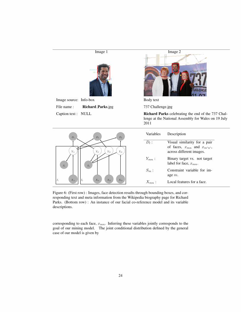
Image 1 Image 2

Image source: Info-box Body text

File name : Richard Parks.jpg 737 Challenge.jpg

Caption text : NULL Richard Parks celebrating the end of the 737 Chal-lenge at the National Assembly for Wales on 19 July2011

D1 D2 D3

Y11 Y21 Y22 Y23

S1 S2

I1 X11 I2 X21 X22 X23

Variables Description

Dl : Visual similarity for a pairof faces, xmn and xm′n′ ,across different images.

Ymn : Binary target vs. not targetlabel for face, xmn.

Sm : Constraint variable for im-age m.

Xmn : Local features for a face.

Figure 6: (First row) : Images, face detection results through bounding boxes, and cor-responding text and meta information from the Wikipedia biography page for RichardParks. (Bottom row) : An instance of our facial co-reference model and its variabledescriptions.

corresponding to each face, xmn. Inferring these variables jointly corresponds to thegoal of our mining model. The joint conditional distribution defined by the generalcase of our model is given by

24

p({{Ymn}Nmn=1}Mm=1, {Dl}Ll=1, {Sm}Mm=1|{{Xmn}Nm

n=1}Mm=1)

=

M∏m=1

Nm∏n=1

p(Ymn|Xmn)p(Sm|{Ymn′}N′m

n′=1)

L∏l=1

p(Dl|{Ym′ln

′l, Ym′′

l n′′l}). (40)

Apart from comparing cross images faces, p(Dl|{Ym′ln

′l, Ym′′

l n′′l}), the joint model

uses predictive scores from per face local binary classifiers, p(Ymn|Xmn). As men-tioned above and discussed in more detail in [9], we used Maximum Entropy Models(MEMs) or Logistic Regression models for these local binary predictions working onmultimedia features in our previous work.

Here, we compare the result of replacing the logistic regression components in themodel discussed above with our BBLR formulation. We examine the impact of thischange in terms of making predictions based solely on independent models taking textand meta-data features as input as well as the impact of this difference when LR vsBBLR models are used as sub-components in the joint structured prediction model.Our hypothesis here is that the BBLR method might improve results due to its robust-ness to outliers (which we have already seen in our binary classification experiments)and that the method is potentially able make more accurate probabilistic predictions,which could in turn lead to more precise joint inference.

Text-only features Joint model with aligned facesMEM 63.4 76.0

BBLR3 67.8 78.2BBLR4 70.2∗ 81.5∗

Table 13: Comparing MEM and BBLRs when used in structured prediction problems.Showing their accuracies (%)

For this particular experiment, we use the biographies with 2-7 faces. Table 13shows results comparing the MaxEnt model with our BBLR model. The results are fora five-fold leave one out of the wikipedia dataset. One can see that we do indeed obtainsuperior performance with the independent BBLR models over the Maximum Entropymodels. We also see improvement to performance when BBLR models are used in thecoupled model where joint inference is used for predictions.

In the row labelled BBLR4, we optimized {w, θB , γ, λ} in addition to other modelparameters using the technique, explained in Section 3.3. This produced statisticallysignificant results compared to the maximum entropy model with p ≤ 0.05. For thissignificance test, we used the McNemar test like our earlier sets of experiments.

25

5.3 Kernel Logistic Regression with the Generalized Beta-BernoulliLoss

In Table 14 we compare Beta-Bernoulli logistic regression with an SVM and KernelBeta-Bernoulli logistic regression (KBBLR). We see that our proposed approach com-pare favorably to the SVM result which is widely considered as a state of the art, strongbaseline.

Table 14: Comparing Kernel BBLR with an SVM and linear BBLR on the standardUCI datasets (no sparsity).

Dataset BBLR SVM KBBLRBreast 2.82 3.26 2.98Heart 17.08 17.76 16.27Liver 31.80 29.61 26.91Pima 21.57 22.44 22.9

5.4 Sparse Kernel BBLRAs shown in [2], one of the advantages of using the ramp loss for kernel based clas-sification is that it can yield models that are even sparser than traditional SVMs basedon the hinge loss. It is well known that L2 based regularization does not typicallyyield sparse solutions when used with traditional kernel logistic regression. Our anal-ysis of the previous experiments reveals that the L2 regularized smooth zero one lossapproximation approach proposed here does not in general lead to sparse models aswell. The well known L1 or lasso regularization method can yield sparse solutions, butoften at the cost of prediction performance. Recently the so called elastic net regular-ization approach [26] based on a weighted combination of L1 and L2 regularizationhas been shown more effective at encouraging sparsity with a less negative impact onperformance. The elastic net approach of course can be viewed as a prior consistingof the product of a Gaussian and a Laplacian distribution. However, part of the mo-tivation for the use of these methods is that they yield convex optimization problemswhen combined with the log logistic loss. Since we have developed a robust approachfor optimizing a non-convex objective function above, this opens the door to the useof non-convex sparsity encouraging regularizers. Correspondingly, we propose andexplore below a prior on parameters, or equivalently, a novel regularization approachbased on a mixture of a Gaussian and a Laplacian distribution. This formulation canbehave like a smooth approximation to an L0 counting “norm” prior on parameters inthe limit as the Laplacian scale parameter goes to zero and the Gaussian variance goesto infinity.

With a (marginalized) Gaussian-Laplace mixture prior, our KBBLR log-likelihood

26

becomes

L(D|a) =n∑i=1

(yi logµi + (1− yi) log(1− µi)

)(41)

+∑j

ln(πgN (aj ; 0, σ

2g) + πlL(aj ; 0, bl)

)where µi = µKβB(a,xi) is our kernel Beta-Bernoulli model as defined in section 3.4,equation (37). For each aj , its prior is modeled through a mixture of a zero mean Gaus-sian N (aj ; 0, σ

2g) with variance σ2

g and a Laplacian distribution L(aj ; 0, bl), located azero with shape parameter bl. For convenience we give the relevant partial derivativesfor this prior in Appendix B. In our approach we also optimize the hyper-parameters{πg, πl, σ2

g , bl} of this prior using hard assignment Expectation Maximization stepsthat are performed after step 3 of Algorithm 2. For precision we outline the steps ofthe modified range-optimization for Kernel BBLR (KBBLR) in Algorithm 3 found inAppendix C.

In Table 15, we compare sparse KBBLR and the SVM using a Radial Basis Func-tion (RBF) kernel. The SVM free parameters were tuned by a cross validation run overthe training data. For a sparse KBBLR solution, we used a mixture of a Gaussian anda Laplacian prior on the kernel weight parameters as presented above.

Table 15: Comparing sparse kernel BBLR with SVMs on the standard UCI evaluationdatasets.

Dataset SVM Avg. Sup-port Vectors

SparseKBBLR

Avg. SupportVectors

Breast 3.26 107 2.83 127Heart 17.76 148 16.40 85Liver 29.61 269 28.74 111Pima 22.44 548 23.52 269

Table 15 compares sparse Kernel BBLR with SVMs on the standard UCI datasets.Figure 7 shows trends in the sparsity curves for an increase in the number of traininginstances comparing KBBLR with SVMs for one of the product review databases. Wecan see that KBBLR scales up well compared to an SVM solution when training datasize increases. Support vectors for SVMs increase almost linearly for an increase in thedatabase size, an effect that has been confirmed in a number of other studies [17, 2]. Incomparison we can see that KBBLR with a Gaussian-Laplacian mixture prior producesa logarithmic curve for an increase in the database size. The right panel of the samefigure also shows the weight distribution before and after the KBBLR optimizationwith a Gaussian-Laplacian mixture prior which yields the observed sparse solution.

27

Figure 7: (left image) Comparing sparse KBBLR with SVMs : the vertical axis showsthe increase in the number of support vectors for an increase in the number of traininginstances (horizontal axis). (right image) This image shows the weight distribution forthe L2 regularized KBBLR (in blue) and the final Gauss-Laplacian mixture solution(in red) at the end of optimization.

6 Discussion and ConclusionsWe have presented a novel formulation for learning with an approximation to the zeroone loss. Through our generalized Beta-Bernoulli formulation, we have provided botha new smooth 0-1 loss approximation method and a new class of probabilistic classi-fiers. Our experimental results indicate that our generalized Beta-Bernoulli formulationis capable of yielding superior performance to traditional logistic regression and maxi-mum margin linear SVMs for binary classification. Like other ramp like loss functionsone of the principal advantages of our approach is that it is more robust dealing withoutliers compared to traditional convex loss functions. Our modified SLA algorithm,which adds a learning hyper-parameter optimization step shows improved performanceover the original SLA optimization algorithm in [14].

We have also presented and explored a kernelized version of our approach whichyields performance competitive with non-linear SVMs for binary classification. Fur-thermore, with a Gaussian-Laplacian mixture prior on parameters our kernel Beta-Bernoulli model is able to yield sparser solutions than SVMs while retaining com-petitive classification performance. Interestingly, for an increase in training databasesize, our approach exhibited logarithmic scaling properties which compares favourablyto the linear scaling properties of SVMs. To the best of our knowledge this is the firstexploration of a Gauss-Laplace mixture prior for parameters – certainly in combinationwith our novel smooth zero-one loss formulation. The ability of this prior to behavelike a smooth approximation to a counting prior is similar to an approach known asbridge regression in statistics. However, our mixture formulation has more flexibilitycompared to the simpler functional form of bridge regression. Interestingly, the com-bination of our generalized Beta-Bernoulli loss with a Gaussian-Laplacian parameterprior can be though of a smooth relaxation to learning with a zero one loss and anL0 counting prior or regularization – a formulation for classification that is intuitivelyattractive, but has remained elusive in practice until now.

28

We also tested our generalized Beta-Bernoulli models for a structured predictiontask arising from the problem of face mining in Wikipedia biographies. Here also ourmodel showed better performance than traditional logistic regression based approaches,both when they were tested as independent models, and when they were compared assub-parts of a Bayesian network based structured prediction framework. This experi-ment shows signs that the model and optimization approach proposed here may havefurther potential to be used in complex structured prediction tasks.

AcknowledgementsWe thank the NSERC Discovery Grants program and Google for a Faculty ResearchAward which helped support this work.

References[1] K. Bache and M. Lichman. UCI machine learning repository, 2013.

[2] R. Collobert, F. Sinz, J. Weston, and L. Bottou. Trading convexity for scalability.In Proceedings of the 23rd international conference on Machine learning, pages201–208. ACM, 2006.

[3] A. Cotter, S. Shalev-Shwartz, and N. Srebro. Learning optimally sparse supportvector machines. In Proceedings of the 30th International Conference on Ma-chine Learning (ICML-13), pages 266–274, 2013.

[4] C. B. Do, Q. Le, C. H. Teo, O. Chapelle, and A. Smola. Tighter bounds forstructured estimation. In Proc. of NIPS, 2008.

[5] M. Dredze, K. Crammer, and F. Pereira. Confidence-weighted linear classifica-tion. In Proceedings of the 25th international conference on Machine learning,pages 264–271. ACM New York, NY, USA, 2008.

[6] S. Ertekin, L. Bottou, and C. L. Giles. Nonconvex online support vector machines.Pattern Analysis and Machine Intelligence, IEEE Transactions on, 33(2):368–381, 2011.

[7] V. Feldman, V. Guruswami, P. Raghavendra, and Y. Wu. Agnostic learning ofmonomials by halfspaces is hard. SIAM Journal on Computing, 41(6):1558–1590, 2012.

[8] K. Gimpel and N. A. Smith. Structured ramp loss minimization for machine trans-lation. In Proceedings of the 2012 Conference of the North American Chapter ofthe Association for Computational Linguistics: Human Language Technologies,pages 221–231. Association for Computational Linguistics, 2012.

[9] M. K. Hasan and C. Pal. Experiments on visual information extraction with thefaces of wikipedia. 2014. AAAI Conference on Artificial Intelligence (AI).

29

[10] R. Herault and Y. Grandvalet. Sparse probabilistic classifiers. In Proceedings ofthe 24th international conference on Machine learning, pages 337–344. ACM,2007.

[11] A. H. Land and A. G. Doig. An automatic method of solving discrete program-ming problems. Econometrica, 28(3):497–520, 1960.

[12] O. L. Mangasarian, W. N. Street, and W. H. Wolberg. Breast cancer diagnosis andprognosis via linear programming. Operations Research, 43(4):570–577, 1995.

[13] L. Mason, J. Baxter, P. Bartlett, and M. Frean. Boosting algorithms as gradientdescent in function space. NIPS, 1999.

[14] T. Nguyen and S. Sanner. Algorithms for direct 0–1 loss optimization in binaryclassification. In Proceedings of the 30th International Conference on MachineLearning (ICML-13), pages 1085–1093, 2013.

[15] F. Perez-Cruz, A. Navia-Vazquez, A. R. Figueiras-Vidal, and A. Artes-Rodriguez.Empirical risk minimization for support vector classifiers. Neural Networks,IEEE Transactions on, 14(2):296–303, 2003.

[16] F. Pernkopf, M. Wohlmayr, and S. Tschiatschek. Maximum margin bayesian net-work classifiers. Pattern Analysis and Machine Intelligence, IEEE Transactionson, 34(3):521–532, 2012.

[17] I. Steinwart. Sparseness of support vector machines. The Journal of MachineLearning Research, 4:1071–1105, 2003.

[18] V. Vapnik. The nature of statistical learning theory. springer, 2000.

[19] P. Vincent. Modeles a noyaux a structure locale. Citeseer, 2004.

[20] P. Vincent and Y. Bengio. Kernel matching pursuit. Machine Learning, 48(1-3):165–187, 2002.

[21] D. Wang, D. Irani, and C. Pu. Evolutionary study of web spam: Webb spam cor-pus 2011 versus webb spam corpus 2006. In Collaborative Computing: Network-ing, Applications and Worksharing (CollaborateCom), 2012 8th InternationalConference on, pages 40–49. IEEE, 2012.

[22] Y. Wu and Y. Liu. Robust truncated hinge loss support vector machines. Journalof the American Statistical Association, 102(479), 2007.

[23] A. L. Yuille and A. Rangarajan. The concave-convex procedure. Neural Compu-tation, 15(4):915–936, 2003.

[24] T. Zhang and F. J. Oles. Text categorization based on regularized linear classifi-cation methods. Information retrieval, 4(1):5–31, 2001.

[25] X. Zhang, A. Saha, and S. Vishwanathan. Smoothing multivariate performancemeasures. Journal of Machine Learning Research, 10:1–55, 2011.

30

[26] H. Zou and T. Hastie. Regularization and variable selection via the elasticnet. Journal of the Royal Statistical Society: Series B (Statistical Methodology),67(2):301–320, 2005.

A Experimental DetailsIn the interests of reproducibility, we also list below the algorithm parameters and therecommended settings as given in [14] :

rR = 2−1, a search radius reduction factor;R0 = 8, the initial search radius;rε = 2−1, a grid spacing reduction factor;εS0

= 0.2, the initial grid spacing for 1-D search;rγ = 10, the gamma parameter reduction factor;γMIN = 2, the starting point for the search over γ;γMAX = 200, the end point for the search over γ.

As a part of the Range Optimization procedure there is also a standard gradient de-scent procedure using a slowly reduced learning rate. The procedure has the followingspecified and unspecified default values for the constants defined below:

rG = 0.1, a learning rate reduction factor;rGMAX

, the initial learning rate;rGMIN

, the minimal learning rate;εL, used for a while loop stopping criterion based on the smallest change in the like-

lihood;εG, used for outer stopping criterion based on magnitude of gradient

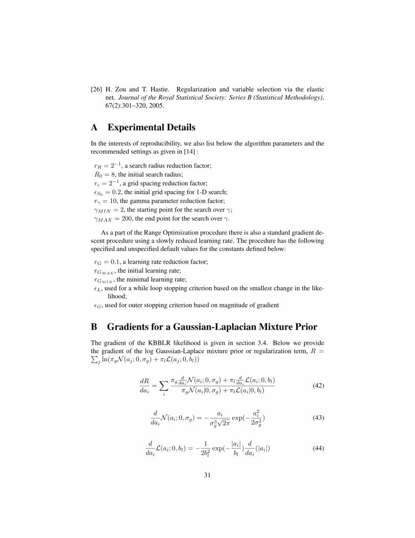
B Gradients for a Gaussian-Laplacian Mixture PriorThe gradient of the KBBLR likelihood is given in section 3.4. Below we providethe gradient of the log Gaussian-Laplace mixture prior or regularization term, R =∑j ln(πgN (aj ; 0, σg) + πlL(aj ; 0, bl))

dR

dai=∑i

πgddaiN (ai; 0, σg) + πl

ddaiL(ai; 0, bl)

πgN (ai|0, σg) + πlL(ai|0, bl)(42)

d

daiN (ai; 0, σg) = −

ai

σ3g

√2π

exp(− a2i2σ2

g

) (43)

d

daiL(ai; 0, bl) = −

1

2b2lexp(−|ai|

bl)d

dai(|ai|) (44)

31

d

dai(|ai|) =

1 if ai > 00 if ai == 0−1 if ai < 0

C Algorithm Modifications for Sparse Gauss-LaplaceKBBLR

Algorithm 3 Range Optimization for Sparse KBBLRInput: w,X, t, γ, radius R, step size εSOutput: Updated estimate for w∗, minimizing 0-1 loss.

1: function GRAD-DESC-IN-RANGE-KBBLR(w,X, t, γ, R, εS)2: repeat

B Stage 1: Find local minimum3: w∗ ← VANILLA-GRAD-DESC(w)

B Stage 2: Sparsify w4: Assign initial near zero weights {wi} to Laplacian cluster, Cl, or to Gaus-

sian cluster, Cg using posterior.5: Estimate priors, {p(Cl(w)), p(Cg(w)}6: repeat7: {πg, πl, σg, bl} ← hyper-parameter updates8: w∗ ← model updates using (41)9: Estimate posteriors {p(Cl|w∗),p(Cg|w∗)}

10: Update clusters, Cl and Cg11: until No clusters change, or a finite # of iterations completed

B Stage 3: Probe each dimension in a radius RB to escape local minimum (if possible)

12: for i = 1 . . . d do . For each dimension, wi13: for step ∈ {εS ,−εS , 2εS ,−2εS , . . . , R,−R} do14: w← w∗

15: wi ← wi + step16: if Lγ(w∗)− Lγ(w) ≥ εL then17: break . Goto step 318: end if19: end for20: end for21: until Lγ(w∗)− Lγ(w) < εL22: return w∗

23: end function

32