a new rate-independent tensorial model for suspensions of ... · not have such a constraint, and...

A new rate-independent tensorial model for suspensions of noncolloidal rigidparticles in Newtonian fluids

Olivier Ozenda,1,2 Pierre Saramito,1,a) and Guillaume Chambon2

1Lab. J. Kuntzmann - CNRS and Univ. Grenoble Alpes, CS 40700 - 38058 Grenoble Cedex 9, France

2Univ. Grenoble Alpes - IRSTEA - UR ETGR, 2 rue de la Papeterie, St-Martin-d’Heres 38402, France

(Received 13 July 2017; final revision received 24 April 2018; published 31 May 2018)

Abstract

We propose a new, minimal tensorial model attempting to clearly represent the role of microstructure on the viscosity of noncolloidal

suspensions of rigid particles. Qualitatively, this model proves capable of reproducing several of the main rheological trends exhibited by

concentrated suspensions: Anisotropic and fore-aft asymmetric microstructure in simple shear and transient relaxation of the microstructure

toward its stationary state. The model includes only few constitutive parameters, with clear physical meaning, that can be identified from

comparisons with experimental data. Hence, quantitative predictions of the complex transient evolution of apparent viscosity observed after

shear reversals are reproduced for a large range of volume fractions. Comparisons with microstructural data show that not only the depletion

angle, but the pair distribution function, are well predicted. To our knowledge, it is the first time that a microstructure-based rheological

model is successfully compared to such a wide experimental dataset.VC 2018 The Society of Rheology.https://doi.org/10.1122/1.4995817

I. INTRODUCTION

Despite the apparent simplicity of the system, concen-

trated suspensions of noncolloidal, rigid spheres in a

Newtonian fluid display a rich and complex rheological

behavior [1–3]. In the inertialess limit (zero Reynolds num-

ber), particle dynamics are essentially governed by hydrody-

namic interactions since lubrication forces prevent, in

principle, direct contacts. Linearity and reversibility of the

Stokes equation then lead to expect that the macroscopic

behavior of the suspension should remain Newtonian. Thus,

numerous investigations documented the increase in the

effective steady-state viscosity of suspensions with particle

volume fraction / [3–5]. However, a wealth of experimental

evidence also showed the existence of non-Newtonian rheo-

logical effects as soon as / exceeds 0.2, typically. One of the

most prominent examples is the existence of transient viscos-

ity drops upon reversal of the shearing direction [6–8]. There

is nowadays a general agreement to relate these non-

Newtonian characteristics to flow-induced changes in the

microstructure of the suspension [3,9,10]. The pair distribu-

tion function gðxÞ, i.e., the likelihood of finding pairs of par-

ticles at a separation vector x, has been shown to become

anisotropic and lose fore-aft symmetry under shear, with

development of preferential concentration and depletion ori-

entations that depend on the volume fraction / [11]. This

asymmetry of the microstructure is the hallmark of a loss of

reversibility of the system that, again, contradicts expecta-

tions based on Stokes equation. Although the precise

mechanisms remain to be elucidated, it is generally inter-

preted as resulting from chaotic dynamics induced by the

nonlinearity of the multibody hydrodynamic interactions

[12], and/or from even weak perturbations of the hydrody-

namic interactions by nonhydrodynamic near-contact forces

[13,14]. Note that the asymmetric microstructure, and the

associated normal stresses, is also at the origin of the cross-

stream particle migration process observed in these suspen-

sions when the shear rate is heterogeneous [15,16].

Since the pioneering work of Einstein [17], most rheolog-

ical models for suspensions assume an additive decomposi-

tion of the total Cauchy stress tensor r into fluid and particle

contributions [2,17,18]. This decomposition naturally arises

from mixture theories in which macroscopic quantities are

obtained from averages over both phases [19–21]. While the

fluid contribution is simply given by a Newtonian model

(with the viscosity of the interstitial fluid), closure relations

are needed to express the particle stresses. Schematically,

two groups of models are found in the literature. The first

group encompasses purely macroscopic approaches that do

not contain explicit reference to the suspension microstruc-

ture, apart from the volume fraction /. The most popular

representative of this class is the suspension balance model

(SBM), introduced in 1994 by Nott and Brady [22] (see also

[15,23]), in which particle stresses are expressed as the sum

of a shear and a normal term that are both linear in shear

rate, with corresponding shear and normal viscosities given

by empirical functions of /. By construction, SBM well

reproduces experimental rheological measurements obtained

in stationary shear. It also leads to realistic predictions con-

cerning particle migration when the particle normal stresses

are used as the driver of the migration flux, even if this

approach has been questioned [21,24]. However, as a

a)Author to whom correspondence should be addressed; electronic mail:

[email protected]

VC 2018 by The Society of Rheology, Inc.J. Rheol. 62(4), 889-903 July/August (2018) 0148-6055/2018/62(4)/889/15/$30.00 889

counterpart for its simplicity, this model is devoid of any

time or strain scale, and therefore unable to account for tran-

sients observed during shear reversal experiments. In addi-

tion, earlier versions were not invariant by changes of

reference frame, although an ad hoc frame-invariant exten-

sion has been proposed [16].

In the second group of models, particle stress is made

explicitly dependent on the microstructure through the con-

sideration of a local conformation tensor that is inspired

from the orientation distribution tensor defined for dilute

fiber suspensions (see, e.g., [25,26]). The conformation ten-

sor, denoted be in this paper, is a second-order symmetric

positive definite tensor describing microstructure anisotropy.

Hand [27] formulated a general representation theorem for

the total Cauchy stress tensor r in terms of the conformation

tensor be and the deformation rate tensor _c. This general rep-resentation should be closed by a constitutive equation for

the evolution of the conformation tensor be. An important

constraint is that the characteristic time associated with the

evolution of be must scale inversely with the deformation

rate j _cj in order to ensure strain-scaling and rate-indepen-dence of the transients, as observed experimentally (see, e.g.,

[8]) and imposed by dimensional analysis [9,28]. Note that

the rate-independence constraint leads to constitutive equa-

tions that are formally similar to hypo-elastic models (see,

e.g., [29]). For concentrated suspensions of spherical par-

ticles, Phan-Thien [30] proposed a differential constitutive

equation for the conformation tensor, that led to prediction

qualitatively in agreement with time-dependent experimental

observations in shear reversal [6,7,31]. The structural unit

used to define the conformation tensor was taken as the unit

vector n joining two neighboring particles, thereby encoding

a direct connection with the pair distribution function gðxÞ.Later, Phan-Thien et al. [32,33] went further with a micro-

macro model inspired from statistical mechanics for the con-

stitutive equation of the conformation tensor, but no quanti-

tative comparisons were obtained. In 2006, Goddard [28]

revisited this approach, and proposed a model involving 12

material parameters and two tensors for describing the

anisotropy. By a systematic fitting procedure of the parame-

ters, he obtained numerical results in quantitative agreement

with shear reversal experiments [7,31]. In 2006, Stickel et al.[34] (see also [35,36]) defined the conformation tensor on

the base of particle mean free path, and simplified the

expression of the stress to be linear in the deformation rate

and the conformation tensor. Their model nevertheless also

involves 13 free parameters. These authors obtained numeri-

cal results in qualitative agreement with a shear reversal

experiment [7,31], but failed to obtain quantitative compari-

sons. In contrast with SBM model, all these tensorial models

are, by construction, frame-invariant and potentially applica-

ble to arbitrary flow geometries and conditions. As for poly-

mer models, normal stress differences naturally arise from

the use of some objective derivative of the conformation ten-

sor be (see [37]). The time-dependent relaxation of this ten-

sor, representing microstructure evolution, leads to transient

responses when the loading is varied. Nevertheless, these

microstructure-based models are still rather complex, and

the identification of parameters is generally not obvious.

This paper is a contribution to an ongoing effort for the

development of more tractable microstructure-based rheo-

logical models. With the least number of adjustable parame-

ters, the proposed model is relatively simple, yet capable of

accounting both for the macroscopic non-Newtonian rheo-

logical features of noncolloidal suspensions and for the rate-

independent evolution of the microstructure. In particular,

this model is able to describe the experimentally observed

anisotropic effects expressed by the pair-distribution func-

tion. It also qualitatively and quantitatively agrees, for a

wide range of volume fraction, with experimental data for

time-dependent shear reversals.

The outline of the paper is as follows: Sec. II concerns the

model statement. Section III deals with predictions in sta-

tionary shear and validation against experimental data for

microstructure anisotropy and depletion angle. Section IV

deals with time-dependent flows, specifically shear reversals,

and present comparisons with experiments for the apparent

viscosity. Finally, Sec. V presents a discussion and a

conclusion.

II. MATHEMATICAL MODEL

A. Rheological model

As illustrated in Fig. 1, a key feature of the microstructure

of sheared suspensions is the existence of preferential direc-

tions along which the average interdistance between particles

varies: Particles are closer along the compression axis and

farther apart along the depletion axis. In inertialess systems,

these preferential directions depend on the concentration /,but not on the deformation rate j _cj (see [11]). The rheologi-

cal model developed in this work is purely macroscopic, and

hence, no attempt is made at deriving a microscopic evolu-

tion equation for the microstructure. However, to clarify the

physical meaning of the conformation tensor be used in the

sequel, and to provide a direct link with the microstructure,

the following definition is proposed:

be ¼ d20h‘� ‘i�1; (1)

where ‘ is the branch vector joining the centers of two neigh-

boring particles, and d0 is the average distance between

neighboring particle centers in an isotropic configuration at

rest. In what follows, the isotropic configuration at rest will

be referred to as the reference configuration. In concentrated

suspensions, d0 is close to 2a, where a denotes particle

radius, since particles are in near-contact. The choice of an

inverse relation between be and h‘� ‘i in Eq. (1) is moti-

vated by the wish to have a conformation tensor whose larg-

est principal direction is aligned with the depletion axis of

the microstructure (Fig. 1). The use of ‘ as the main micro-

structural unit is notably different from the approach fol-

lowed in most earlier studies, which define a fabric tensor

hn� ni based on the unit vector joining neighboring par-

ticles, n ¼ ‘=j‘j [3,28,32,33,38]. In particular, while the

trace of the tensor hn� ni is by construction equal to one,

the h‘� ‘i tensor and the present be conformation tensor do

890 OZENDA, SARAMITO, AND CHAMBON

not have such a constraint, and thus present additional

degrees of freedom.

To couple the conformation tensor be with a rheological

model, we introduce a deformation ce defined as

ce ¼ be � I;

where I is the identity tensor. For an isotropic microstructure at

rest, i.e., the reference configuration, we have be ¼ I, and thus,

ce ¼ 0. Hence, ce can be interpreted as the average deformation

of the local cages formed by neighboring particles, with respect

to the reference configuration. Note that a similar concept of

cages formed by nearest neighbors was already introduced in

[34]. We then assume that the total deformation of the suspen-

sion c can be decomposed into the sum of the cage deformation

ce and of a viscous deformation cv, which represents the global

rearrangements of neighboring particles through the flow

c ¼ ce þ cv: (2)

The next step is to write a constitutive equation for the vari-

able ce. To that aim, we define a local stress, denoted as se,

and assume the following relation between se and ce:

se ¼ ggj _cjce; (3)

where the tensorial norm jnj is defined as jnj ¼ ½ð1=2Þn : n�1=2for any second-order tensor n. Observe that this expression is

linear with respect to ce and involves a factor ggj _cj that

ensures rate-independence of the constitutive relation. Here,

gg is a constant coefficient with the dimension of a viscosity.

This local stress se is also assumed to be linearly related to the

rate of viscous deformation _cv through

se ¼ ge _cv; (4)

where ge P 0 is an associated viscosity. Finally, differentiat-

ing Eq. (2), replacing _cv from Eq. (4) and using Eq. (3), the

following linear differential equation is obtained for ce:

_ce þggge

j _cj ce ¼ _c:

The previous constitutive equation is completed by the fol-

lowing expression for the total Cauchy stress tensor of the

suspension:

r ¼ �pf I þ g _c þ s;

where s ¼ ggj _cjce þ gdðce � ceÞ : _c:

The first term involves pf, the pressure in the fluid phase. The

second term represents the base viscosity of the suspension,

expressed here by gP0. Finally, the third term represents the

microstructure stress s. This microstructure stress itself

expresses as the sum of the local stress se and of a quadratic

term with respect to ce. Such quadratic terms commonly

derive from the closure of a fourth-order structure tensor in

statistical micro-macro models for spherical or fiber suspen-

sions (see, e.g., [25,26]). It involves an additional parameter

gd with the dimension of a viscosity. Note that this last term

writes equivalently gdð _c : ceÞce and, thus, the two tensors s

and ce are colinear and share the same eigensystem. The

influence of this additional quadratic contribution will be

analyzed in the following.

In the present model, the total stress is thus split into the

stress that would be observed for an isotropic microstructure

(the base viscosity), and the stress induced by the anisotropic

arrangement of the microstructure (represented by s).

This stress decomposition could appear similar to the

decomposition r ¼ rf þ rp between fluid rf and particle rp

FIG. 1. (left) Schematic representation of the branch vectors ‘ joining neighboring particles in a sheared suspension. (right) Representation of the local confor-mation tensor be by an ellipse. The compression axis is the line and the depletion axis is the dashed line. In the electronic version they are drawn in red and in

green, respectively. Background photography taken from [39], Fig. 4.7 (/ ¼ 0:55).

891A NEW NONCOLLOIDAL SUSPENSION MODEL

stresses, used in classical mixture theories [20] and in most

suspensions models, such as SBM [10,22]. It shall be empha-

sized however that, in our approach, the base viscosity g also

contains a contribution from the particle phase. More pre-

cisely, for the present model, we have rf ¼ �pf I þ g0 _c and

rp ¼ ðg� g0Þ _c þ s, where g0 is the viscosity of the

suspending fluid. Roughly, the base viscosity g can be seen

as accounting for long-range hydrodynamic interactions

between particles, while the microstructure stress s accounts

for short-range, hydrodynamic and contact, interactions.

As a consequence, we expect all the parameters of the

model, including g, ge, gg, and gd to depend on the

volume fraction /. Finally, also recall that trðceÞ, and

thus trðsÞ, are not necessarily zero, such that the microstruc-

ture stress s may also contribute to the total pressure

p ¼�ð1=3ÞtrðrÞ of the suspension. Indeed, p ¼ pf þ pp withpp ¼ �ð1=3ÞtrðrpÞ ¼ �ð1=3ÞtrðsÞ, as the mixture is assumed

to be isochoric with trð _cÞ ¼ 0.

The time derivative _ce is given by the upper-convected

tensor derivative (see, e.g., [37], chap 4), denoted hereafter

Dce=Dt

DceD t

¼ @ce@t

þ ðu:rÞce �ruce � ceruT :

The deformation rate _c is identified to two times the

symmetric part of the velocity gradient tensor

DðuÞ ¼ ðruþruTÞ=2, where u is the velocity field of the

mixture. The constitutive equations thus become

2DðuÞ ¼ DceDt

þ aj2DðuÞj ce; (5a)

r¼�pf Iþ2gDðuÞþge aj2DðuÞjþbðDðuÞ : ceÞ

� �ce; (5b)

where a ¼ gg=ge and b ¼ 2gd=ge are dimensionless parame-

ters. These constitutive equations can be seen as a rate-

independent variant of a viscoelastic Oldroyd [40]

model with an additional quadratic term for the total stress.

Rate-independence is guaranteed by the use of an “effective

elastic modulus” ggj _cj proportional to the deformation rate.

B. Problem statement

Coupling the above constitutive model with the mass and

momentum conservation equations of the mixture, the prob-

lem can be formulated as a system of three equations for

three unknowns: ce, the particle cage deformation; u, themixture velocity; and pf, the pressure in the fluid phase

DceDt

þ aj2DðuÞj ce � 2DðuÞ ¼ 0; (6a)

qDu

Dt� div �pf I þ 2gDðuÞ

� �

�div geceðaj2DðuÞj þ bðDðuÞ : ceÞÞ� �

¼ qg;(6b)

div u ¼ 0: (6c)

The isochoric relation (6c) of the mixture is a consequence

of mass conservation of the fluid and solid phases. From a

mathematical point of view, the fluid pressure pf acts as a

Lagrange multiplier associated with this isochoric constraint.

The problem is closed by suitable initial and boundary condi-

tions. In Eq. (6b), D=Dt ¼ @=@tþ u:r denotes the Lagrange

derivative and q is the density of the mixture. From Hulsen

[41], it is possible to show that the constitutive equation (6a)

leads to a conformation tensor be ¼ I þ ce that is always

positive definite. Note that the volume fraction /, and hence

q, is supposed to be constant during the flow: In agreement

with experimental evidences [3], we assume the time scale

for migration to be large compared to the typical time scales

for microstructure evolution, and focus here on the short-

time response of the suspensions. Otherwise, the system

could also be coupled with an additional diffusion equation

for the volume fraction [23].

III. STATIONARY SHEAR FLOWS ANDMICROSTRUCTURE ANISOTROPY

Let us consider a simple shear flow. The x axis is in the

flow direction and the y axis is in the direction of the gradientr ¼ ð0; @y; 0Þ. Let uðt; x; y; zÞ ¼ ðuxðt; yÞ; 0; 0Þ be the veloc-

ity and _cðtÞ ¼ @yux be the spatially uniform shear rate. The

constitutive equations (5a) and (5b) become, after expanding

the upper-convected derivative [37] (chap. 4)

@tce;xy þ aj _cjce;xy ¼ _c; (7a)

@tce;xx � 2 _cce;xy þ aj _cjce;xx ¼ 0; (7b)

@tce;yy þ aj _cjce;yy ¼ 0; (7c)

@tce;zz þ aj _cjce;zz ¼ 0; (7d)

rxy ¼ agej _cjce;xy þ bge _cc2e;xy þ g _c; (7e)

rxx ¼ agej _cjce;xx þ bge _cce;xyce;xx; (7f)

completed by an initial condition for ce. For simplicity, we

assume an isotropic microstructure at t¼ 0. Hence, ce;yyð0Þ¼ ce;zzð0Þ ¼ 0, which yields ce;yyðtÞ ¼ ce;zzðtÞ ¼ 0 for all

t> 0. Similarly, ce;xzð0Þ ¼ ce;yzð0Þ ¼ 0.

We first focus on a stationary simple shear flow where the

shear rate is supposed to be constant and is denoted _c0. Inthat case, the solution writes explicitly

ce;xy ¼ sgnð _c0Þa�1; ce;xx ¼ 2a�2; (8a)

rxy ¼ gþ ð1þ ba�2Þge� �

_c0; (8b)

rxx ¼ 2a�1ð1þ ba�2Þgej _c0j: (8c)

Observe that the model predicts a normal stress component

proportional to the shear rate j _c0j. This feature is in agree-

ment with several experimental observations [4]. In contrast,

most classical viscoelastic models, such as Maxwell and

Oldroyd models, predict normal stresses in shear flows


proportional to _c20 [37] (p. 157). In the present model, normal

stresses proportional to j _c0j arise from the use in Eq. (3) of

an effective elastic modulus that is itself proportional to j _c0j,as required to obtain a rate-independent rheological behav-

ior. The particle pressure pp ¼ �trðsÞ=3 is given by, for the

present stationary simple shear flow

pp ¼ �ð2=3Þa�1ð1þ ba�2Þgej _c0j: (8d)

Thus, pp is also proportional to the shear rate j _c0j, again in

agreement with experimental observations [42]. Finally note

that, from Eq. (8b), the shear stress component rxy also

scales linearly with _c0, as expected.Let us now turn to microstructural aspects, described by

the particle cage deformation tensor ce. As we only con-

sider stationary simple flows in this paragraph, we can

assume without loss of generality that _c0 > 0. From Eq.

(8a), the eigenvector associated with the largest eigenvalue

of the tensor ce makes an angle with the x axis denoted as

he and given by

he ¼ atan�1þ

ffiffiffiffiffiffiffiffiffiffiffiffiffi1þ a2

p

a

� �¼ 1

2atanðaÞ

() a ¼ tanð2heÞ:(9)

Since be ¼ I þ ce, the tensors be and ce share the same

eigensystem. The angle he is thus also associated with larg-

est eigenvalue of be, i.e., to the dilation direction of the

microstructure: In this direction, the probability to find two

particles in contact is the smallest, and he thus correspondsto the so-called depletion angle. Experimental data for the

depletion angle he versus volume fraction / are presented

by Blanc [39], Fig. 5.11, and are reproduced in Fig. 2 (left),

together with a best fit using a second-order polynomial

denoted by heð/Þ. Assuming heð0Þ ¼ 0 and heð/mÞ ¼ p=4,with /m the maximum volume fraction of the suspension, the

second-order polynomial template can be expressed as

heð/Þ ¼ de/þ p4� de/m

� �//m

� �2

; (10)

where /m ¼ 0:571 and de ¼ 0:661 are adjusted through a

nonlinear least square method, as implemented in gnuplot[43]. Through Eq. (9), the dependence upon / of the aparameter of the present model is thus directly deduced from

the experimental data (see Fig. 2, right)

að/Þ ¼ tan 1:32/þ 2:48/2� �

: (11)

In experiments or in numerical simulations, the microstruc-

ture of suspensions is generally represented through the pair

distribution function gðxÞ. As an example, Fig. 3 shows, for

a suspension at / ¼ 0:35 submitted to a stationary shear

flow, the experimentally determined evolution of gðxÞ in the

shear plane (x, y) [11]. Recall that gðxÞ is the conditional

probability, when there is already a particle in x0 ¼ 0, to find

a particle at any location x 2 R2, normalized by the average

particle density /=ð4pa3=3Þ (where a is particle radius).

Observe in Fig. 3 that g is zero in the central disk of diameter

2a, due to nonpenetration of particles. It is maximum in a

thin band ½2a; 2aþ d� and then tends to 1 when the distance

increases. Most of the relevant microstructure information is

encoded in this thin band, whose thickness d is sufficient to

include contact and near-contact interactions, and which thus

describes the average arrangement of neighboring particles

FIG. 2. (left) Depletion angle he versus volume fraction /: Experimental data from [39], Fig. 5.11, and best fit with the second-order polynomial (10). (right)

Dependence upon / of model parameter a.


[9,10]. Switching to polar coordinates ðr; hÞ in the shear

plane, we assume, in order to simplify the modeling of g,that this function only depends upon h in the thin band. We

thus introduce its average value, denoted as ~gðhÞ, in the

radial direction in the thin band, and the associated probabil-

ity distribution function pðhÞ such that

pðhÞ ¼ ~gðhÞðp

�p~gðhÞ dh

:

This distribution pðhÞ is interpreted as the probability to find,

for each particle in the suspension, a neighboring particle in

the h direction inside the thin band. Assuming furthermore

that the probability to find a neighboring particle outside the

thin band is negligible, pðhÞ can be related to the fabric ten-

sor hn� ni introduced in Sec. II A as follows:

hn� ni ¼ðh¼p

h¼�pn� n pðhÞ dh; (12)

where nðhÞ ¼ ðcos h; sin hÞ is the unit outward normal vector

to the unit circle. Observe that, as expected,

tr hn� ni ¼ðp

�ppðhÞ dh ¼ 1

since p is a probability distribution. Accordingly, from Eq.

(1), we can thus postulate the following relation between pðhÞand the conformation tensor be introduced in our model:

ðh¼p

h¼�pn� n pðhÞ dh ¼ b�1

e

tr b�1e

� � : (13)

As shown in Appendix A, for a given conformation tensor

be, Eq. (13) can be used to reconstruct the probability distri-

bution pðhÞ through a Fourier mode decomposition.

From Eq. (13), the first Fourier mode of pðhÞ can be

expressed explicitly in terms of the parameter a and the

depletion angle he: See Appendix A, relation (A3). This pre-

diction is compared in Fig. 4 with experimental data from

Blanc [39], Figs. 5.9 and 5.10. Observe that both predicted

(in black) and experimental (in dotted-red) curves present

two main lobes, separated by the depletion angle direction.

The experimental probability distribution is however also

affected by higher-frequency modes, which are potentially

very sensitive to both experimental errors from image pre-

processing and the choice of the width of the thin band

½2a; 2aþ d� used to integrate the pair distribution function,

as pointed out by Blanc [39], Fig. 5.6. Figure 5 represents

the five first Fourier coefficients of the experimental data.

Observe in general the rapid decrease in these coefficients,

as expected. However, when the volume fraction / becomes

close to the maximal fraction /m, the second mode domi-

nates. A similar behavior has already been experimentally

observed for dry granular material [44] and can be explained

by steric exclusion of neighbors. This second Fourier mode

cannot be determined by the present model, as explained in

Appendix A.

IV. TIME-DEPENDENT SIMPLE SHEAR FLOWS

A. Shear startup, reversal and pause

For simple shear flows, the problem reduces to the time-

dependent linear system of ordinary differential equations

(7a)–(7f). For a constant applied shear rate _c0, the system

can be explicitly solved by performing the change of variable

c ¼ j _c0jt, where c represents the deformation. The solution

writes

ce;xyðcÞ ¼ 1� e�acð Þsgnð _c0Þa�1 þ e�ac; (14a)

ce;xxðcÞ ¼ 1� e�acð Þ2a�2 þ e�acce;xyð0Þ� fce;xxð0Þ þ 2cðsgnð _c0Þce;xyð0Þ� a�1Þg; (14b)

and, then, the total tress tensor r is explicitly given in Eqs.

(7e) and (7f).

For a startup from a material at rest at t¼ 0 with an isotro-

pic microstructure, we have ceð0Þ ¼ 0. If a constant shear rate

_c0 > 0 is imposed for t> 0, the solutions (14a)–(14b) become

ce;xyðcÞ ¼ 1� e�acð Þa�1;

ce;xxðcÞ ¼ 1� e�acð Þ2a�2 � e�ac2a�1c:

As shown in Fig. 6, this solution displays an exponential

relaxation toward the steady state solution. Remark that the

graph of the solution versus shear deformation c ¼ _c0t is

invariant when changing the value of shear rate _c0 > 0. This

constitutes a fundamental property of rate-independent

materials.

Let us now turn to a case of shear reversal: The material

is first sheared with a negative shear rate � _c0 until a first sta-tionary regime is reached. Then, at t¼ 0, the shear rate is

suddenly reversed to the opposite value þ _c0 > 0. In that

FIG. 3. Pair distribution function g(x, y): Experimental observation by

Blanc et al. [11] for a stationary shear flow with / ¼ 0:35.


case, ce;xyð0Þ ¼ �a�1, ce;xxð0Þ ¼ 2a�2 and the solutions

(14a) and (14b) become

ce;xyðcÞ ¼ 1� 2e�acð Þa�1;

ce;xxðcÞ ¼ 1� e�acð Þ2a�2 þ e�acð2a�2 � 4a�1cÞ:

As shown in Fig. 7, at t¼ 0, the particle cages, represented

by the conformation tensor be ¼ I þ ce as an ellipse, start

to rotate toward a symmetrically opposite position.

According to Eq. (9), the depletion angle increases from

heð0Þ ¼ �atanðaÞ=2 at t¼ 0 to reach asymptotically its new

value heð1Þ ¼ þatanðaÞ=2. With the choice a ¼ffiffiffi3

pmade

FIG. 5. Five first Fourier coefficients pk, kP1 of the probability distribution function pðhÞ, from experimental data by Blanc [39], Fig. 5.10, for / ¼ 0:3, 0.4,and 0.5.

FIG. 4. Probability distribution function pðhÞ, represented in polar coordinates as r ¼ pðhÞ. Comparison between model prediction (black curve) and experi-

mental data (red dotted-curves) by Blanc [39], Fig. 5.10. The experimental pdfs are obtained as radial averages of the pair distribution function in the thin band

corresponding to r=a 2 ½1:87; 2:14�. The depletion angle is indicated by an arrow and its value is given in degrees. The dotted blue circle represents the equi-

probable (isotropic) distribution pðhÞ ¼ 1=ð2pÞ.


in Fig. 7, we have heð1Þ ¼ p=6. The depletion angle is

expressed at any c ¼ _c0t from the ce tensor components by

heðcÞ ¼ atan�ce;xxðcÞ þ

ffiffiffiffiffiffiffiffiffiffiffiffiffiffiffiffiffiffiffiffiffiffiffiffiffiffiffiffiffiffiffiffiffiffiffiffic2e;xxðcÞ þ 4c2e;xyðcÞ

q

ce;xyðcÞ

0@

1A:

A Taylor development for small ce;xyðcÞ shows that heðcÞvanishes when ce;xyðcÞ ¼ 0, i.e., when the shear deformation

is equal to the critical value c� ¼ a�1 log ð2Þ. For this criticaldeformation, the ellipse axis associated with the largest

eigenvalue (in green in Fig. 7), is horizontal with ce;xyðc�Þ ¼ 0

and ce;xxðc�Þ ¼ 2ð1� log ð2ÞÞa�2 > 0. It means that the

microstructure temporarily presents a fore-aft symmetry, but

is not isotropic, i.e., be 6¼ I when c ¼ c�. Figure 7 also plots

separately the two components ce;xy and ce;xx of the tensor:

Observe that trðceÞ ¼ ce;xx is not constant during the reversal.

This constitutes an important difference with approaches

based on a fabric tensor hn� ni that always has trace equal toone [3,28,32,33,38].

For a general _cðtÞ evolution, the system of ordinary dif-

ferential equations (7a)–(7f) is solved using lsode library

[45], as interfaced in octave software [46]. Figure 8 plots

the response in stress components and depletion angle

when applying a succession of startups and reversals, possi-

bly separated by pauses. In agreement with experimental

observations [7] (Fig. 3), when the imposed shear rate

changes from _c0 6¼ 0 to zero, i.e., during a pause, both parti-

cle pressure pp ¼ �trðsÞ=3 ¼ �sxx=3 and shear stress rxyinstantaneously fall to zero. Observe however that the

depletion angle remains constant during the pause: The

microstructure is conserved. This latter feature can be

deduced from constitutive equation (5a), which simply

reduces to Dce=Dt ¼ 0 when the shear rate is zero. After a

pause, if the shear restarts suddenly in the same direction,

experimental observations [7] (Fig. 3) showed that both

particle pressure pp ¼ �sxx=3 and shear stress rxy jump

instantaneously to their previous stationary values.

Conversely, if the shear rate restarts suddenly in the direc-

tion opposite to its previous value, e.g., � _c0, experimental

observations by Narumi et al. [31], Fig. 3, showed that par-

ticle pressure pp progressively increases from zero to its

previous stationary value while shear stress rxy progres-

sively decreases from zero to the opposite of its previous

stationary value. As shown in Fig. 8, all these features are

remarkably well captured by the present model.

The apparent viscosity of the suspension is defined as

gapp ¼ rxy= _c. From Eq. (7e), we obtain

FIG. 8. Shear evolution with pauses, startups, and reversals: Evolution of

imposed shear rate, depletion angle, and stress components versus shear

deformation (choice of parameters: a ¼ffiffiffi3

p, b¼ 5, ge ¼ 10 Pa s, and

g¼ 10 Pa s).

FIG. 6. Shear startup from rest: Exponential relaxation of the ce tensor com-

ponents versus shear deformation c ¼ _c0t (with a ¼ffiffiffi3

p).

FIG. 7. Shear reversal at t¼ 0: evolution versus shear deformation c ¼ _c0tof the conformation tensor be ¼ I þ ce represented as an ellipse.

Eigenvector associated to compression (resp. dilation), i.e. to the smallest

(resp. largest) eigenvalue of be, is represented as the smallest (resp. largest)

axis. In the electronic version it is drawn in red (resp. green). On the bottom,

plots for the depletion angle heðtÞ, and the ce tensor components versus

shear deformation c ¼ _c0t. (Parameter a is taken asffiffiffi3

pin this plot.)


gappðcÞ ¼ gþ gece;xyðcÞ aþ bce;xyðcÞ� �

: (15)

Notice that the apparent viscosity is independent of the

shear rate. Figure 9 presents the evolution of the apparent

viscosity for a shear reversal, together with a sensitivity

analysis to the model parameters. The apparent viscosity

shows three regimes after the shear reversal: First, an

instantaneous decrease is observed. The apparent viscosity

then continues to decrease with a smooth shape until a min-

imum is reached. Finally, the apparent viscosity increases

and relaxes exponentially to its stationary value. As shown

in Fig. 9, these different regimes are diversely affected by

the model parameters a, b, ge, and g. The parameter a con-

trols the relaxation of the solution to its stationary value:

The larger a, the faster the solution reaches the stationary

regime. In fact, a�1 interprets as a characteristic deforma-

tion for reaching the stationary regime. The parameter bcontrols the existence of the smooth minimum and the

shape of the curve around this minimum. When b¼ 0, there

is no smooth minimum, and the apparent viscosity is mono-

tonically increasing immediately after the shear reversal.

The viscosity ge influences the stationary plateau, while the

minimum remains unchanged. Finally, the parameter g

globally shifts the apparent viscosity: Note that this effect

is obvious when considering Eq. (15).

B. Comparison with experiments

We quantitatively compared our model to the unsteady

shear flow experiments of Blanc [39], sec 3.3 (see also

[8,11,47]). This author performed shear reversal experiments

in a Couette rheometer. The suspensions were prepared with

polymethyl methacrylate (PMMA) spherical particles in a

Newtonian oil at various volume fractions / ranging from

0.30 to 0.50. The experiments were performed at an imposed

torque whose value was adjusted in order to obtain, for each

volume fraction, similar angular velocities in the stationary

regime. All geometrical and material parameters of the

experiments are summarized in Table I. Note that, experi-

mentally, the suspensions have been found to be slightly

shear-thinning, with a power index on the order 0.9 (see

[39]). This slight shear-thinning is not considered in the fol-

lowing comparison with our model.

Neglecting the variations inside the gap, we assume the

shear rate as uniform and consider this experiment as a sim-

ple shear flow. The problem is then described again in Eqs.

FIG. 9. Apparent viscosity during shear reversal: Sensitivity of the response to the model parameters (base value of the parameters: a ¼ffiffiffi3

p, b¼ 5, ge ¼ 10 Pa

s, and g¼ 10 Pa s).


(7a)–(7f), where now rxy is imposed and _c is unknown.

Observe that, based on relation (7e), the unknown shear rate

_c expresses explicitly in terms of the unknown ce;xy and the

given data rxy (see Appendix B). This expression can then be

inserted in Eq. (7a), yielding a nonlinear scalar ordinary dif-

ferential equation for ce;xy. This equation does not admit, to

our knowledge, an explicit solution and should be solved

numerically. As in the previous paragraph, the numerical

procedure uses lsode library [45].

The present model involves four parameters that need to be

determined: a, b, ge, and g. The a parameter has already been

identified for this experimental setup, and its dependence upon

/ is given in Eq. (11). For each volume fraction, identification

of the three other parameters can be performed based on the

evolution of the apparent viscosity gapp ¼ rxy= _c during the

shear reversals, as illustrated in the previous sensitivity analysis.

Figure 10 presents direct comparisons between model

prediction and experimental measurements of the apparent

viscosity. Observe that the sudden decrease in the apparent

viscosity the after shear reversal, and its relaxation to the sta-

tionary value, is qualitatively and quantitatively very well

reproduced by the present continuous model, and this for the

different volume fractions investigated. For / ¼ 0:47, theapparent viscosity measured during the experiments displays

a very slowly increasing trend for large deformations c. Thisfeature, which is obviously not captured by the model, could

be due to slow migration of the particles induced by the

small variations of the shear rate in the Couette gap.

Table II summarizes, for each volume fraction, the values of

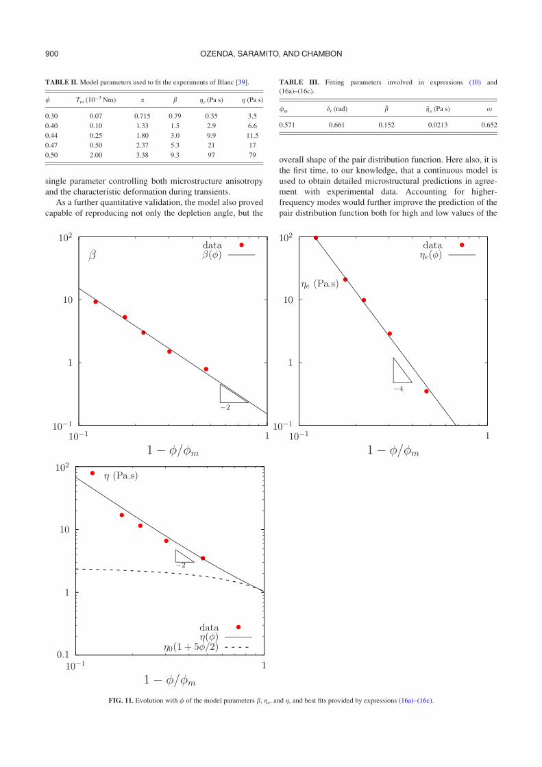
the four adjustable parameters a, b, ge and g provided by the fit-ting. Figure 11 shows the dependency upon / of the parameters

b, ge and g. The regularity of these dependencies suggests the

existence of material functions with the following forms:

bð/Þ ¼ �b 1� //m

� ��2

; (16a)

geð/Þ ¼ �ge 1� //m

� ��4

; (16b)

gð/Þ ¼ g0 1� xþ 5

2� 2x/m

� �/

� �

þ g0x 1� //m

� ��2

: (16c)

Hence, b and ge vs / are expressed by simple power-law

dependencies diverging at / ¼ /m, where /m is the maxi-

mum volume fraction of the suspension. Expression (16c)

for gð/Þ is an original extension of Krieger and Dougherty

[48]’s rule, associated with the –2 power-law index, where xis a balance parameter. Note that, when the volume fraction

is small, the first order development of Eq. (16c) coincides

with Einstein [17]’s rule gð/Þ=g0 ¼ 1þ 5/=2þ Oð/2Þ for

any value of /m and x 2 ½0; 1�. Best-fitted values of all the

material parameters involved in Eqs. (16a)–(16c) are indi-

cated in Table III. Finally, recall that the evolution of a upon

/ was obtained independently, and is given in Eq. (11).

V. DISCUSSION AND CONCLUSIONS

This paper proposes a minimal tensorial model attempting

to clearly represent the role of microstructure on the apparent

viscosity of noncolloidal suspensions of rigid particles. The

contribution to the total stress of the suspension of local aniso-

tropic particle arrangements, is accounted for through a spe-

cific microstructure stress. This microstructure stress is

expressed as a function of a local conformation tensor, whose

evolution is governed by a rate-independent viscoelasticlike

differential equation. Qualitatively, this model proves capable

of reproducing several important non-Newtonian trends exhib-

ited by concentrated suspensions. First, the development of an

anisotropic, and fore-aft asymmetric, microstructure in simple

shear is well captured by the conformation tensor. As

expected, the stationary microstructure is independent of shear

rate [see Eq. (9)]. The depletion angle, which corresponds to

the largest eigenvalue of the conformation tensor, is a function

of a single model parameter a that can be adjusted to fit exper-imental observations. Second, in time-dependent cases, the

model predicts transient responses associated with the pro-

gressive relaxation of the microstructure toward its stationary

state. In agreement with experimental observations, these tran-

sient responses occur for shear reversals (due to the associated

reversal of anisotropy direction), but not for changes of shear

rate with the same sign (since microstructure is rate-indepen-

dent). Also in agreement with experiments, the microstructure

remains frozen during shear pauses, and its evolution during

the transients is fully controlled by the shear deformation. The

critical deformation to reach the stationary regime is directly

related, again, to the parameter a.Overall, the model presented here includes only 4 consti-

tutive parameters. Besides a, two viscosities g and ge repre-sent the base viscosity of the suspension for an isotropic

microstructure and the excess viscosity induced by micro-

structure anisotropy, respectively, while the nonlinearity

parameter b controls the early stage of the transients. This

limited number of parameters, and their clear physical mean-

ing, is an advantage compared to most previous

microstructure-based rheological models proposed in the lit-

erature [28,32,34]. In particular, parameter identification for

quantitative comparisons with experimental data is relatively

straightforward. We showed that the model is capable of

quantitatively reproducing the complex transient evolution

of apparent viscosity observed after shear reversals for a

TABLE I. Parameters of the shear reversal experiments of Blanc [39].

Description Unit Symbol Value

Fluid viscosity Pa S g0 1.03

Outer radius m Re 2.4 � 10-2

Inner radius m Ri 1.4� 10-2

Height m L 4.5 � 10-2

Torque N m Tm Imposed

Angular velocity s�1 x Measured

Shear stress Pa rxy0:818� Tm2pLR2

c

Shear rate s�1 _c xRi

Re�Ri


large range of volume fractions. Both the immediate

response, characterized by an instantaneous drop followed

by a smooth minimum, and the subsequent exponential

relaxation are well captured. Note that the quadratic term in

Eq. (5b), and the parameter b, is essential to obtain the

smooth minimum observed in experimental data. To our

knowledge, it is the first time that a microstructure-based

rheological model is successfully compared to such a wide

experimental data set. This comparison allowed us to derive

material functions for the evolution of the constitutive

parameters with volume fraction. Noteworthy, the values of

the parameter a were determined from microstructure data

(depletion angle), and then applied without adjustment to

model the transient response. This validates the use of a

FIG. 10. Shear reversal: Apparent viscosity gapp vs deformation c. Comparison between experimental measurements from Blanc [39] for a suspension of

PMMA particles in a Couette geometry and computations with the present model. For each volume fraction /, the three model parameters b, ge, and g were

obtained through a best-fit procedure. Parameter values are indicated in Table II.


single parameter controlling both microstructure anisotropy

and the characteristic deformation during transients.

As a further quantitative validation, the model also proved

capable of reproducing not only the depletion angle, but the

overall shape of the pair distribution function. Here also, it is

the first time, to our knowledge, that a continuous model is

used to obtain detailed microstructural predictions in agree-

ment with experimental data. Accounting for higher-

frequency modes would further improve the prediction of the

pair distribution function both for high and low values of the

FIG. 11. Evolution with / of the model parameters b, ge, and g, and best fits provided by expressions (16a)–(16c).

TABLE III. Fitting parameters involved in expressions (10) and

(16a)–(16c).

/m de (rad) �b �ge (Pa s) x

0.571 0.661 0.152 0.0213 0.652

TABLE II.Model parameters used to fit the experiments of Blanc [39].

/ Tm (10�3 Nm) a b ge (Pa s) g (Pa s)

0.30 0.07 0.715 0.79 0.35 3.5

0.40 0.10 1.33 1.5 2.9 6.6

0.44 0.25 1.80 3.0 9.9 11.5

0.47 0.50 2.37 5.3 21 17

0.50 2.00 3.38 9.3 97 79


volume fraction, but would require the consideration of

higher-order structure tensors in the model. Other promising

prospects include the addition of a friction term to the micro-

structure stress, which could prove important for modeling

volume fractions close to /m and/or experiments performed

at an imposed particle pressure [49].

Future works shall also consider in more details the issue

of normal stresses. Indeed, another important non-

Newtonian rheological feature exhibited by noncolloidal sus-

pensions is the development of normal stress differences in

simple shear flow, with negative values of N2, an ongoing

debate concerning the sign of N1, and a ratio jN2=N1j on the

order of three, typically [4,50–53]. In agreement with experi-

mental observations, our model effectively predicts that

microstructure anisotropy is associated with the existence of

normal stresses proportional to shear rate. However, expres-

sions of stresses in simple shear lead to N2 ¼ 0 and N1 > 0

[see Eq. (8c)]. As a consequence, the particle pressure pp,expressed in Eq. (8d), has a sign opposite to that expected.

This indicates that, although the minimal model presented

here is capable to reproduce microstructure evolutions, addi-

tional degrees of freedom would be needed to capture the

full rheological behavior of suspensions. These improve-

ments will be required to consider, e.g., more complex non-

viscosimetric flows such as extensional flows [54] or flows

around an obstacle [55,56]. These improvements are also

required in order to predict particle migration, by consider-

ing the microstructure stress s as the driver of the particle

flux, through an approach analogous to SBM [16].

ACKNOWLEDGMENTS

The authors thank Fr�ed�eric Blanc, �Elisabeth Lemaire,

Laurent Lobry, and Francois Peters for fruitful discussions

about the rheology of suspensions and for providing us data

files of experimental measurements used in this paper for

comparison with our model. The authors would also like to

thank the three anonymous reviewers for their careful

reading of the paper and their constructive comments.

APPENDIX A: COMPUTATION OF THEPROBABILITY DISTRIBUTION FUNCTION

Let l6 be the two eigenvalues of the fabric tensor

hn� ni, with l�6lþ and e� ¼ ðcos ðheÞ; sin ðheÞÞ and eþ¼ ð�sin ðheÞ; cos ðheÞÞ the two corresponding eigenvectors,

where he is the depletion angle. Expressing Eq. (12) in the

eigenbasis, observing that n:e� ¼ cos ðh� heÞ and n:eþ¼ sin ðh� heÞ, we get

ðp

�pcos2ðh� heÞ pðhÞ dh ¼ l�; (A1a)

ðp

�psin2ðh� heÞ pðhÞ dh ¼ lþ: (A1b)

Note that, by construction, pðhÞ is even (see Fig. 3). Then,

expressing pðhÞ in terms of a Fourier series as:

pðhÞ ¼X

kP0

pk cos ð2kðh� heÞÞ;

where pk 2 R; kP0 are the Fourier coefficients, we obtain

from Eqs. (A1a) and (A1b), after computation of the inte-

grals, that p0 ¼ 1=ð2pÞ and p1 ¼ �ðlþ � l�Þ=ð2pÞ. The

coefficients pk for kP2 remain undetermined. Observe from

Fig. 5 that, in experimental data, these coefficients present a

fast decrease. By retaining only the two first coefficients, the

present model is able to predict the following probability

distribution:

pðhÞ ¼ 1

2p1� ðlþ � l�Þ cos f2ðh� heÞg� �

: (A2)

Note that such expression was previously used by Troadec

et al. [44], Eq. (1). Remark that he minimizes pðhÞ: As

expected, the depletion angle is the direction where the prob-

ability to find a neighbor particle is minimal.

In the present model, the fabric tensor is expressed from

Eq. (13) by hn� ni ¼ b�1e =trðb�1

e Þ with be ¼ I þ ce.

Accordingly, the two eigenvalues of the fabric tensor hn� niare

lþ ¼ ð1þ k�Þ�1

ðkþ þ 1Þ�1 þ ðk� þ 1Þ�1;

l� ¼ ð1þ kþÞ�1

ðkþ þ 1Þ�1 þ ðk� þ 1Þ�1;

where k6 denotes the two eigenvalues of ce. From Eq. (8a), we

have k6 ¼ 16ffiffiffiffiffiffiffiffiffiffiffiffiffi1þ a2

p� �=a2. Then lþ � l� ¼ 1=

ffiffiffiffiffiffiffiffiffiffiffiffiffi1þ a2

p

and the previous relation (A2) writes explicitly in terms of the

model parameter a only

pðhÞ ¼ 1

2p1� 1ffiffiffiffiffiffiffiffiffiffiffiffiffi

1þ a2p cos ð2ðh� heÞÞ

� �; (A3)

where he is expressed explicitly versus a in Eq. (9).

APPENDIX B: SYSTEM OF ODE FOR IMPOSEDSTRESS

Assuming a strictly positive apparent viscosity, we have

sgnð _cðtÞÞ ¼ sgnðrxyðtÞÞ for all time tP0 and relation (7e)

leads to the following explicit expression of the shear rate _cversus the given shear stress rxy and the unknown ce;xy:

_cðtÞ¼rxyðtÞ

gþge asgnðrxyðtÞÞce;xyðtÞþbc2e;xyðtÞ� � when rxyðtÞ6¼0

0 otherwise:

8>><>>:

(B1)

This expression of the shear rate _c is replaced in Eqs. (7a)

and (7b) and we then obtain a nonlinear ordinary differential

equations (ODE) in terms of the two unknowns ce;xy and

ce;xx. These EDO are closed by two initial conditions

ce;xyð0Þ ¼ sgnðrxyð0ÞÞ a�1 and ce;xxð0Þ ¼ 2a�2. For the shear


reversal, rxyð0Þ is chosen and rxyðtÞ ¼ �rxyð0Þ for all t> 0.

For the shear reversal experiments of Blanc [39] with an

imposed torque Tm, rxyð0Þ is given in Table I. After compu-

tation of ce;xy and ce;xx, the rate of deformation _cðsÞ is com-

puted from Eq. (B1), and finally, the deformation cðtÞ is

obtained by a numerical integration asÐ t0j _cðsÞjds.

References

[1] Stickel, J. J., and R. L. Powell, “Fluid mechanics and rheology of

dense suspensions,” Ann. Rev. Fluid Mech. 37, 129–149 (2005).

[2] Guazzelli, E., and J. F. Morris, A Physical Introduction to Suspension

Dynamics (Cambridge University, UK, 2012).

[3] Denn, M. M., and J. F. Morris, “Rheology of non-Brownian sus-

pensions,” Ann. Rev. Chem. Biomol. Eng. 5, 203–228 (2014).

[4] Zarraga, I. E., D. A. Hill, and D. T. Leighton, Jr., “The characterization

of the total stress of concentrated suspensions of noncolloidal spheres

in Newtonian fluids,” J. Rheol. 44, 185–220 (2000).

[5] Ovarlez, G., F. Bertrand, and S. Rodts, “Local determination of the

constitutive law of a dense suspension of noncolloidal particles

through magnetic resonance imaging,” J. Rheol. 50, 259–292

(2006).

[6] Gadala-Maria, F., and A. Acrivos, “Shear-induced structure in a con-

centrated suspension of solid spheres,” J. Rheol. 24, 799–814

(1980).

[7] Kolli, V. G., E. J. Pollauf, and F. Gadala-Maria, “Transient normal

stress response in a concentrated suspension of spherical particles,”

J. Rheol. 46, 321–334 (2002).

[8] Blanc, F., F. Peters, and E. Lemaire, “Local transient rheological

behavior of concentrated suspensions,” J. Rheol. 55, 835–854

(2011).

[9] Brady, J. F., and J. F. Morris, “Microstructure of strongly sheared sus-

pensions and its impact on rheology and diffusion,” J. Fluid Mech.

348, 103–139 (1997).

[10] Morris, J. F., “A review of microstructure in concentrated suspensions

and its implications for rheology and bulk flow,” Rheol. Acta 48,

909–923 (2009).

[11] Blanc, F., E. Lemaire, A. Meunier, and F. Peters, “Microstructure in sheared

non-Brownian concentrated suspensions,” J. Rheol. 57, 273–292 (2013).

[12] Drazer, G., J. Koplik, B. Khusid, and A. Acrivos, “Deterministic and

stochastic behaviour of non-Brownian spheres in sheared sus-

pensions,” J. Fluid Mech. 460, 307–335 (2002).

[13] Metzger, B., and J. E. Butler, “Irreversibility and chaos: Role of long-

range hydrodynamic interactions in sheared suspensions,” Phys. Rev.

E 82, 051406 (2010).

[14] Gallier, S., E. Lemaire, F. Peters, and L. Lobry, “Rheology of sheared

suspensions of rough frictional particles,” J. Fluid Mech. 757, 514–549

(2014).

[15] Morris, J. F., and F. Boulay, “Curvilinear flows of noncolloidal suspen-

sions: The role of normal stresses,” J. Rheol. 43, 1213–1237 (1999).

[16] Miller, R. M., J. P. Singh, and J. F. Morris, “Suspension flow modeling

for general geometries,” Chem. Eng. Sci. 64, 4597–4610 (2009).

[17] Einstein, A., “Eine neue bestimmung der molek€uldimensionen,” Ann.

Phys. Ser. 4(19), 289–306 (1906).

[18] Einstein, A., Investigation on the Theory of the Brownian Movement

(Dover, Mineola, NY, USA, 1956).

[19] Jackson, R., “Locally averaged equations of motion for a mixture of

identical spherical particles and a Newtonian fluid,” Chem. Eng. Sci.

52, 2457–2469 (1997).

[20] Jackson, R., The Dynamics of Fluidized Particles (Cambridge

University, UK, 2000).

[21] Nott, P. R., E. Guazzelli, and O. Pouliquen, “The suspension balance

model revisited,” Phys. Fluids 23, 043304 (2011).

[22] Nott, P. R., and J. F. Brady, “Pressure-driven flow of suspensions:

Simulation and theory,” J. Fluid Mech. 275, 157–199 (1994).

[23] Miller, R. M., and J. F. Morris, “Normal stress-driven migration and

axial development in pressure-driven flow of concentrated sus-

pensions,” J. Non-Newtonian Fluid Mech. 135, 149–165 (2006).

[24] Lhuillier, D., “Migration of rigid particles in non-Brownian viscous

suspensions,” Phys. Fluids 21, 023302 (2009).

[25] Lipscomb, G. G., M. M. Denn, D. U. Hur, and D. V. Boger, “The flow

of fiber suspensions in complex geometries,” J. Non-Newtonian Fluid

Mech. 26, 297–325 (1988).

[26] Reddy, B. D., and G. P. Mitchell, “Finite element analysis of fibre sus-

pension flows,” Comput. Meth. Appl. Mech. Eng. 190, 2349–2367

(2001).

[27] Hand, G. L., “A theory of anisotropic fluids,” J. Fluid Mech. 13, 33–46

(1962).

[28] Goddard, J. D., “A dissipative anisotropic fluid model for non-

colloidal particle dispersions,” J. Fluid Mech. 568, 1–17 (2006).

[29] Kolymbas, D., “An outline of hypoplasticity,” Arch. Appl. Mech. 61,

143–151 (1991).

[30] Phan-Thien, N., “Constitutive equation for concentrated suspensions

in Newtonian liquids,” J. Rheol. 39, 679–695 (1995).

[31] Narumi, T., H. See, Y. Honma, T. Hasegawa, T. Takahashi, and N.

Phan-Thien, “Transient response of concentrated suspensions after

shear reversal,” J. Rheol. 46, 295–305 (2002).

[32] Phan-Thien, N., X.-J. Fan, and B. C. Khoo, “A new constitutive model

for monodispersed suspensions of spheres at high concentrations,”

Rheol. Acta 38, 297–304 (1999).

[33] Phan-Thien, N., X.-J. Fan, and R. Zheng, “A numerical simulation of

suspension flow using a constitutive model based on anisotropic inter-

particle interactions,” Rheol. Acta 39, 122–130 (2000).

[34] Stickel, J. J., R. J. Phillips, and R. L. Powell, “A constitutive model for

microstructure and total stress in particulate suspensions,” J. Rheol.

50, 379–413 (2006).

[35] Stickel, J. J., R. J. Phillips, and R. L. Powell, “Application of a consti-

tutive model for particulate suspensions: Time-dependent viscometric

flows,” J. Rheol. 51, 1271–1302 (2007).

[36] Yapici, K., R. L. Powell, and R. J. Phillips, “Particle migration and

suspension structure in steady and oscillatory plane Poiseuille flow,”

Phys. Fluids 21, 053302 (2009).

[37] Saramito, P., Complex Fluids: Modelling and Algorithms (Springer

International Publishing AG, Cham, Switzerland, 2016).

[38] Chacko, R. N., R. Mari, S. M. Fielding, and M. E. Cates, “Shear rever-

sal in dense suspensions: The challenge to fabric evolution models

from simulation data,” J. Fluid Mech. (to be published).

[39] Blanc, F., “Rh�eologie et microstructure des suspensions concentr�ees

non Browniennes,” Ph.D. thesis, Universit�e Nice Sophia Antipolis

(2011).

[40] Oldroyd, J. G., “On the formulation of rheological equations of states,”

Proc. R. Soc. Lond. A 200, 523–541 (1950).

[41] Hulsen, M. A., “A sufficient condition for a positive definite configura-

tion tensor in differential models,” J. Non-Newtonian Fluid Mech. 38,

93–100 (1990).

[42] Deboeuf, A., G. Gauthier, J. Martin, Y. Yurkovetsky, and J. F. Morris,

“Particle pressure in a sheared suspension: A bridge from osmosis to

granular dilatancy,” Phys. Rev. Lett. 102, 108301 (2009).

[43] Williams, T., and C. Keley, “Gnuplot: An interactive program,”

(2010), http://www.gnuplot.info.

[44] Troadec, H., F. Radjai, S. Roux, and J. C. Charmet, “Model for granu-

lar texture with steric exclusion,” Phys. Rev. E 66, 041305 (2002).


[45] Radhakrishnan, K., and A. C. Hindmarsh, “Description and use of

LSODE, the Livermore solver for ordinary differential equations,”

Technical Report No. UCRL-ID-113855, LLNL (1993).

[46] Eaton, J. W., D. Bateman, and S. Hauberg, Octave: A High-Level

Interactive Language for Numerical Computations (Free Software

Foundation, 2011), http://www.gnu.org/software/octave.

[47] Blanc, F., F. Peters, and E. Lemaire, “Experimental signature of the

pair trajectories of rough spheres in the shear-induced microstructure

in noncolloidal suspensions,” Phys. Rev. Lett. 107, 208302 (2011).

[48] Krieger, I. M., and T. J. Dougherty, “A mechanism for non-Newtonian flow

in suspensions of rigid spheres,” Trans. Soc. Rheol. 3, 137–152 (1959).

[49] Boyer, F., �E. Guazzelli, and O. Pouliquen, “Unifying suspension and

granular rheology,” Phys. Rev. Lett. 107, 188301 (2011).

[50] Boyer, F., O. Pouliquen, and �E. Guazzelli, “Dense suspensions in

rotating-rod flows: Normal stresses and particle migration,” J. Fluid

Mech. 686, 5–25 (2011).

[51] Couturier, �E., F. Boyer, O. Pouliquen, and �E. Guazzelli, “Suspensions

in a tilted trough: Second normal stress difference,” J. Fluid Mech.

686, 26–39 (2011).

[52] Dai, S.-C., E. Bertevas, F. Qi, and R. I. Tanner, “Viscometric functions

for noncolloidal sphere suspensions with Newtonian matrices,”

J. Rheol. 57, 493–510 (2013).

[53] Dbouk, T., L. Lobry, and E. Lemaire, “Normal stresses in concentrated

non-Brownian suspensions,” J. Fluid Mech. 715, 239–272 (2013).

[54] Dai, S., and R. I. Tanner, “Elongational flows of some non-colloidal

suspensions,” Rheol. Acta 56, 63–71 (2017).

[55] Haddadi, H., S. Shojaei-Zadeh, K. Connington, and J. F. Morris,

“Suspension flow past a cylinder: Particle interactions with recirculat-

ing wakes,” J. Fluid Mech. 760, R2 (2014).

[56] Dbouk, T., “A suspension balance direct-forcing immersed boundary

model for wet granular flows over obstacles,” J. Non-Newtonian Fluid

Mech. 230, 68–79 (2016).


a new rate-independent tensorial model for suspensions of ... · not have such a constraint, and...

Documents