A new point matching algorithm for non-rigid

registration

Haili Chui a

aR2 Technologies

Sunnyvale, CA 94087

e-mail: hchui@r2tech.com

Anand Rangarajan b

bDept. of Computer and Information Science & Engineering

University of Florida, Gainesville, FL 32611-6120

e-mail: anand@cise.ufl.edu

Abstract

Feature-based methods for non-rigid registration frequently encounter the corre-spondence problem. Regardless of whether points, lines, curves or surface parame-terizations are used, feature-based non-rigid matching requires us to automaticallysolve for correspondences between two sets of features. In addition, there could bemany features in either set that have no counterparts in the other. This outlierrejection problem further complicates an already difficult correspondence problem.We formulate feature-based non-rigid registration as a non-rigid point matchingproblem. After a careful review of the problem and an in-depth examination of twotypes of methods previously designed for rigid robust point matching (RPM), wepropose a new general framework for non-rigid point matching. We consider it ageneral framework because it does not depend on any particular form of spatialmapping. We have also developed an algorithm—the TPS-RPM algorithm—withthe thin-plate spline (TPS) as the parameterization of the non-rigid spatial map-ping and the softassign for the correspondence. The performance of the TPS-RPMalgorithm is demonstrated and validated in a series of carefully designed syntheticexperiments. In each of these experiments, an empirical comparison with the pop-ular iterated closest point (ICP) algorithm is also provided. Finally, we apply thealgorithm to the problem of non-rigid registration of cortical anatomical structureswhich is required in brain mapping. While these results are somewhat preliminary,they clearly demonstrate the applicability of our approach to real world tasks in-volving feature-based non-rigid registration.

Key words: registration, non-rigid mapping, correspondence, feature-based,softassign, thin-plate splines (TPS), robust point matching (RPM), linearassignment, outlier rejection, permutation matrix, brain mapping

Preprint submitted to Elsevier Science 14 October 2002

1 Introduction

Feature-based registration problems frequently arise in the domains of com-puter vision and medical imaging. With the salient structures in two imagesrepresented as compact geometrical entities (e.g. points, curves, surfaces), theregistration problem is to find the optimum or a good sub-optimal spatialtransformation/mapping between the two sets of features. The point feature,represented by feature location is the simplest form of feature. It often servesas the basis upon which other more sophisticated representations (such ascurves, surfaces) can be built. In this sense, it can also be regarded as themost fundamental of all features. However, feature-based registration usingpoint features alone can be quite difficult.

One common factor is the noise arising from the processes of image acquisi-tion and feature extraction. The presence of noise means that the resultingfeature points cannot be exactly matched. Another factor is the existence ofoutliers—many point features may exist in one point-set that have no cor-responding points (homologies) in the other and hence need to be rejectedduring the matching process. Finally, the geometric transformations may needto incorporate high dimensional non-rigid mappings in order to account fordeformations of the point-sets. Consequently, a general point feature registra-tion algorithm needs to address all these issues. It should be able to solve forthe correspondences between two point-sets, reject outliers and determine agood non-rigid transformation that can map one point-set onto the other.

The need for non-rigid registration occurs in many real world applications.Tasks like template matching for hand-written characters in OCR, generatingsmoothly interpolated intermediate frames between the key frames in cartoonanimation, tracking human body motion in motion tracking, recovering dy-namic motion of the heart in cardiac image analysis and registering humanbrain MRI images in brain mapping, all involve finding the optimal transfor-mation between closely related but different objects or shapes. It is such acommonly occurring problem that many methods have been proposed to at-tack various aspects of the problem. However, because of the great complexityintroduced by the high dimensionality of the non-rigid mappings, all existingmethods usually simplify the problem to make it more tractable. For example,the mappings can be approximated by articulated rigid mappings instead ofbeing fully non-rigid. Restricting the point-sets to lie along curves, the setof correspondence can be constrained using the curve ordering information.Simple heuristics such as using nearest-neighbor relationships to assign corre-spondence [as in the iterated closest point algorithm (Besl and McKay, 1992)]

2

have also been widely used. Though most methods tolerate a certain amountof noise, they normally assume that there are no outliers. These simplificationsmay alleviate the difficulty of the matching problem, but they are not alwaysvalid. The non-rigid point matching problem, in this sense, still remains un-solved. Motivated by these observations, we feel that there is a need for a newpoint matching algorithm that can solve for non-rigid mappings as well as thecorrespondences in the presence of noise and outliers.

Our approach to non-rigid point matching closely follows our earlier work onjoint estimation of pose and correspondence using the softassign and deter-ministic annealing (Gold et al., 1998; Rangarajan et al., 1997; Chui et al.,1999). This work was developed within an optimization framework and re-sulted in a robust point matching (RPM) algorithm which was restricted tousing affine and piecewise-affine mappings. Here, we extend the frameworkto include spline-based deformations and develop a general purpose non-rigidpoint matching algorithm. Furthermore, we develop a specific algorithm—TPS-RPM—wherein we adopt the thin-plate spline (TPS) (Wahba, 1990;Bookstein, 1989) as the non-rigid mapping. The thin-plate spline is chosenbecause it is is the only spline that can be cleanly decomposed into affine andnon-affine subspaces while minimizing a bending energy based on the secondderivative of the spatial mapping. In this sense, the TPS can be considered tobe a natural non-rigid extension of the affine map.

The rest of the paper is organized as follows. A detailed review of relatedwork is presented in the next section. The optimization approach culminatingin the TPS-RPM algorithm is developed in Section 3. This is followed byvalidation experiments using synthetic examples and a preliminary evaluationof the algorithm in the field of brain mapping. We then conclude by pointingout possible extensions of the present work.

2 Previous Work

There are two unknown variables in the point matching problem—the corre-spondence and the transformation. While solving for either variable withoutinformation regarding the other is quite difficult, an interesting fact is thatsolving for one variable once the other is known is much simpler than solvingthe original, coupled problem.

Methods that solve only for the spatial transformation: The method ofmoments (Hibbard and Hawkins, 1988) is a classical technique which tries tosolve for the transformation without ever introducing the notion of correspon-dence. The center of mass and the principal axis can be determined by momentanalysis and used to align the point sets. A more sophisticated technique is

3

the Hough Transform (Ballard, 1981; Stockman, 1987). The transformationparameter space is divided into small bins, where each bin represents a cer-tain configuration of transformation parameters. The points are allowed tovote for all the bins and the transformation bin which get the most votes ischosen. There are other methods, e.g., tree searches (Baird, 1984; Grimsonand Lozano-Perez, 1987), the Hausdorff distance (Huttenlocher et al., 1993),geometric hashing (Lamdan et al., 1988; Hummel and Wolfson, 1988) and thealignment method (Ullman, 1989). These methods work well for rigid trans-formations. However, these methods cannot be easily extended to the caseof non-rigid transformations where the number of transformation parametersoften scales with the cardinality of the data set. We suspect that this is themain reason why there is relatively a dearth of literature on non-rigid pointmatching despite a long and rich history on rigid, affine and projective pointmatching (Grimson, 1990).

Methods that solve only for the correspondence: A different approachto the problem focuses on determining the right correspondence. As a bruteforce method, searching through all the possible point correspondences is ob-viously not possible. Even without taking into consideration the outliers, thisleads to a combinatorial explosion. Certain measures have to be taken to prunethe search in correspondence space. There are three major types of methodsdesigned to do just that.

The first type of method, called dense feature-based methods, tries to groupthe feature points into higher level structures such as lines, curves or surfacesthrough object parameterization. Then, the allowable ways in which the objectcan deform is specified (Metaxas et al., 1997; Sclaroff and Pentland, 1995). Inother words, curves and/or surfaces are first fitted to features extracted fromthe images (Tagare et al., 1995; Metaxas et al., 1997; Szeliski and Lavallee,1996; Feldmar and Ayache, 1996). Very often, a common parameterized coor-dinate frame is used in the fitting step, thereby alleviating the correspondenceproblem. The advantages and disadvantages can be clearly seen in the curvematching case. With the extra curve ordering information now available, thecorrespondence space can be drastically reduced making the correspondenceproblem much easier. On the other hand, the requirement of such extra in-formation poses limitations for these methods. These methods work well onlywhen the curves to be matched are reasonably smooth. Also, the curve fittingstep that precedes matching is predicated on good feature extraction. Bothcurve fitting and feature extraction can be quite difficult when the data arenoisy or when the shapes involved become complex. Most of these methodscannot handle multiple curves or partially occluded curves.

The second type of method works with more sparsely distributed point-sets.The basic idea is that while a point-set of a certain shape is non-rigidly deform-ing, different points at different locations can be assigned different attributes

4

depending on their ways of movement. These movement attributes are used todistinguish the points and determine their correspondences. Following Scottand Longuet-Higgins (1991) and Shapiro and Brady (1992); Cootes et al.(1995), the modal matching approach in Sclaroff and Pentland (1995) usesa mass and stiffness matrix that is built up from the Gaussian of the dis-tances between point features in either point-set. The mode shape vectors areobtained as the eigenvectors of the decoupled dynamic equilibrium equations,which are defined using the above matrices. The correspondence is computedby comparing each point’s relative participation in the eigen-modes. One ma-jor limitation of these algorithms is that they cannot tolerate outliers. Outlierscan cause serious changes to the deformation modes invalidating the result-ing correspondences. The accuracy of the correspondence obtained by justcomparing the eigen-modes may also be limited.

The third type of approach recasts point matching as inexact, weighted graphmatching (Shapiro and Haralick, 1981). Here, the spatial relationships betweenthe points in each set are used to constrain the search for the correspondences.In Cross and Hancock (1998), such inter-relationships between the points istaken into account by building a graph representation from Delaunay trian-gulations. An expectation-maximization (EM) algorithm is used to solve theresulting graph matching optimization problem. However, the spatial map-pings are restricted to be affine or projective. As we shall see, our approach inthis work shares many similarities with Cross and Hancock (1998). In Amitand Kong (1996), decomposable graphs are hand-designed for deformable tem-plate matching and minimized with dynamic programming. In Lohmann andvon Cramon (2000), a maximum clique approach is used to match relationalsulcal graphs. In either case, there is no direct relationship between the de-formable model and the graph used. The graph definition is also a commonproblem because inter-relationships, attributes and link type information canbe notoriously brittle and context dependent. In fact, the graphs in Amit andKong (1996); Lohmann and von Cramon (2000) are hand designed.

Methods that solve for both the correspondence and the transfor-mation: Solving for the correspondence or the transformation alone seemsrather difficult, if not impossible. Note that it is much easier to estimate thenon-rigid transformation once the correspondence is given. On the other hand,knowledge of a reasonable spatial transformation can be of considerable helpin the search for correspondence. This observation points to another way ofsolving the point matching problem—alternating estimation of correspondenceand transformation.

The iterative closest point (ICP) algorithm (Besl and McKay, 1992) is the sim-plest of these methods. It utilizes the nearest-neighbor relationship to assigna binary correspondence at each step. This estimate of the correspondence isthen used to refine the transformation, and vice versa. It is a very simple and

5

fast algorithm which is guaranteed to converge to a local minimum. Underthe assumption that there is an adequate set of initial poses, it can becomea global matching tool for rigid transformations. Unfortunately, such an as-sumption is no longer valid in the case of non-rigid transformations, especiallywhen then the deformation is large. ICP’s crude way of assigning correspon-dence generates a lot of local minima and does not usually guarantee thatthe correspondences are one-to-one. Its performance degenerates quickly withoutliers, even if some robustness control is added (Rangarajan et al., 1997;Chui et al., 1999).

Recognizing these drawbacks of treating the correspondence as strictly a bi-nary variable, other approaches relax this constraint and introduce the notionof “fuzzy” correspondence. There are mainly two kinds of approaches. In Wells(1997); Cross and Hancock (1998); Hinton et al. (1992) a probabilistic approachis used. Point matching is modeled as a probability density estimation problemusing a Gaussian mixture model. The well known expectation-maximization(EM) algorithm is used to solve the matching problem. When applied to thepoint matching problem, the E-step basically estimates the correspondenceunder the given transformation, while the M-step updates the transformationbased on the current estimate of the correspondence. In Wells (1997), the out-liers are handled through a uniform distribution in addition to the Gaussianmixture model. A similar digit recognition algorithm proposed in Hinton et al.(1992) models handwritten digits as deformable B-splines. Such a B-spline aswell as an affine transformation are solved to match a digit pair. However,both Wells (1997); Cross and Hancock (1998) only solve for rigid transforma-tions. Designed for character recognition, the approach in Hinton et al. (1992)assumes that the data points can be represented by B-splines and does notaddress the issue of matching arbitrary point patterns. One other commonproblem shared by all the probabilistic approaches is that they do not enforceone-to-one correspondence. In our previous work (Gold et al., 1998; Rangara-jan et al., 1997; Chui et al., 1999), point matching is modeled as a joint linearassignment-least squares optimization problem—a combination of two classicalproblems. Two novel techniques, namely deterministic annealing and softas-sign, were used to solve the joint optimization problem. Softassign used withindeterministic annealing guarantees one-to-one correspondence. The resultingalgorithm is actually quite similar to the EM algorithm.

Another approach recently proposed in Belongie et al. (2002) adopts a differ-ent probabilistic strategy. A new shape descriptor, called the “shape context”,is defined for correspondence recovery and shape-based object recognition.For each point chosen, lines are drawn to connect it to all other points. Thelength as well as the orientation of each line are calculated. The distributionof the length and the orientation for all lines (they are all connected to thefirst point) is estimated through histogramming. This distribution is used asthe shape context for the first point. Basically, the shape context captures

6

the distribution of the relative positions between the currently chosen pointand all other points. The shape context is then used as the shape attributefor the chosen point. The correspondence can then be decided by comparingeach point’s attributes in one set with the attributes in the other. Since at-tributes and not relations are compared, the search for correspondence can beconducted much more easily. Or in more technical terms, the correspondenceis obtained by solving a relatively easier bipartite matching problem ratherthan a more intractable (NP-complete) graph matching problem (Gold andRangarajan, 1996a). After the correspondences are obtained, the point set iswarped and the method repeated. Designed with the task of object recognitionin mind, this method has demonstrated promising performance in matchingshape patterns such as hand-written characters. However, it is unclear howwell this algorithm works in a registration context. Note that from a shapeclassification perspective, only a distance measure needs to be computed forthe purposes of indexing. In contrast, in a registration setting, an accurateestimation of the spatial mapping is paramount. In addition, the convergenceproperties of this algorithm are unclear since there is no global objective func-tion that is being minimized. Nonetheless, shape context may prove to be auseful way of obtaining attribute information which in turn helps in disam-biguating correspondence.

The choice of the non-rigid transformation: As mentioned above, wechoose the TPS to parameterize the non-rigid transformation. The TPS wasdeveloped in Wahba (1990) as a general purpose spline tool which generates asmooth functional mapping for supervised learning. The mapping is a singleclosed-form function for the entire space. The smoothness measure is definedas the sum of the squares of the second derivatives of the mapping functionover the space. Bookstein (1989) pioneered the use of TPS to generate smoothspatial mappings between two sets of points with known one-to-one corre-spondences (landmarks) in medical images. Due to the limitation of knowncorrespondence, use of the TPS has been restricted. The primary goal of thispaper is to remove the limitation of known correspondence.

3 Point Matching as Joint Estimation of Correspondence and theSpatial Mapping

3.1 A Binary Linear Assignment-Least Squares Energy Function

Suppose we have two point-sets V and X (in <2or in <3) consisting of points{va, a = 1, 2, . . . , K} and {xi, i = 1, 2, . . . , N} respectively. For the sake ofsimplicity, we will assume for the moment that the points are in 2D.

7

zai x1 x2 x3 x4 outlier

v1 1 0 0 0 0

v2 0 1 0 0 0

v3 0 0 0 0 1

outlier 0 0 1 1

Fig. 1. An Example of the Binary Correspondence Matrix: Points v1 and v2

correspond to x1 and x2 respectively, and the rest of the points are outliers. Notethat the existence of an extra outlier row and outlier column makes it possible forthe row and column constraints to always be satisfied.

We represent the non-rigid transformation by a general function f . A pointva is mapped to a new location ua = f(va). The whole transformed point-set V is then U or {ua}. We use a smoothness measure to place appropriateconstraints on the mapping. To this end, we introduce an operator L and ourchosen smoothness measure is ||Lf ||2. We discuss this issue in greater detailin Section 4 where we specialize f to the thin-plate spline.

We now motivate the energy function used for non-rigid point matching. Wewould like to match the point-sets as closely as possible while rejecting areasonable fraction of the points as outliers. The correspondence problem iscast as a linear assignment problem (Papadimitriou and Steiglitz, 1982), whichis augmented to take outliers into account. The benefit matrix in the linearassignment problem depends on the non-rigid transformation. More formally,our goal in this work is to minimize the following binary linear assignment-least squares energy function:

minZ,f

E(Z, f) = minZ,f

N∑

i=1

K∑

a=1

zai||xi − f(va)||2 + λ||Lf ||2 − ζN∑

i=1

K∑

a=1

zai (1)

subject to∑N+1

i=1 zai = 1 for i ∈ {1, 2, . . . , N}, ∑K+1a=1 zai = 1 for a ∈ {1, 2, . . .K}

and zai ∈ {0, 1}. The matrix Z or {zai} is the binary correspondence matrix(Gold et al., 1998; Rangarajan et al., 1997) consisting of two parts. The innerN × K part of Z defines the correspondence. If a point va corresponds to apoint xi, zai = 1, otherwise zai = 0. The row and column summation con-straints guarantee that the correspondence is one-to-one. The extra N + 1th

row and K + 1th column of Z are introduced to handle the outliers. Oncea point is rejected as an outlier, the extra entries will start taking non-zerovalues to satisfy the constraints, when the related inner entries all becomezero. (An example of the correspondence matrix is given in Figure 1.) Thesecond term is our constraint on the transformation. The third term is therobustness control term preventing rejection of too many points as outliers.The parameters λ and ζ are the weight parameters that balance these terms.

8

Posed in this manner, the point matching objective function in (1) consists oftwo interlocking optimization problems: a linear assignment discrete problemon the correspondence and a least-squares continuous problem on the trans-formation. Both problems have unique solutions when considered separately.It is their combination that makes the non-rigid point matching problem diffi-cult. Since the correspondence (transformation) has an optimal solution whenthe transformation (correspondence) is held fixed, it is natural to consider analternating algorithm approach. However, even if such an approach is used,solving for binary one-to-one correspondences (and outliers) at each step isnot meaningful when the transformation is far away from the optimal solution.Consequently, we have adopted an alternating algorithm approach where thecorrespondences are not allowed to approach binary values until the transfor-mation begins to converge to a reasonable solution. This is done with the helpof two techniques—softassign and deterministic annealing, which have beenpreviously used to solve such joint optimization problems (Gold et al., 1998;Rangarajan et al., 1997; Chui et al., 1999). It is also similar to the dual-stepEM algorithm in Cross and Hancock (1998) wherein a similar alternating al-gorithm approach is used. Note that in Cross and Hancock (1998), there is noattempt to solve for non-rigid deformations.

3.2 Softassign and Deterministic Annealing

The basic idea of the softassign (Gold et al., 1998; Rangarajan et al., 1997;Chui et al., 1999) is to relax the binary correspondence variable Z to be acontinuous valued matrix M in the interval [0, 1], while enforcing the rowand column constraints. The continuous nature of the correspondence matrixM basically allows fuzzy, partial matches between the point-sets V and X.From an optimization point of view, this fuzziness makes the resulting energyfunction better behaved (Yuille and Kosowsky, 1994) because the correspon-dences are able to improve gradually and continuously during the optimizationwithout jumping around in the space of binary permutation matrices (andoutliers). The row and column constraints are enforced via iterative row andcolumn normalization (Sinkhorn, 1964) of the matrix M .

With this notion of fuzzy correspondence established, another very useful tech-nique, deterministic annealing (Yuille, 1990; Gold et al., 1998), can be usedto directly control this fuzziness by adding an entropy term in the form ofT

∑N+1i=1

∑K+1a=1 mai log mai to the original assignment energy function (1). The

newly introduced parameter T is called the temperature parameter. The namecomes from the fact that as you gradually reduce T , the energy function isminimized by a process similar to physical annealing (Yuille, 1990). At highertemperatures, the entropy term forces the correspondence to be more fuzzyand hence becomes a factor in “convexifying” the objective function. The min-

9

ima obtained at each temperature are used as initial conditions for the nextstage as the temperature is lowered. This process of deterministic annealingis a useful heuristic in a variety of optimization problems (Geiger and Girosi,1991; Gold and Rangarajan, 1996b; Hofmann and Buhmann, 1997).

3.3 A Fuzzy Linear Assignment-Least Squares Energy Function

After introducing these two techniques, the original binary assignment-leastsquares problem is converted to the problem of minimizing the following fuzzyassignment-least squares energy function (Gold et al., 1998; Rangarajan et al.,1997; Chui et al., 1999):

E(M, f) =N∑

i=1

K∑

a=1

mai||xi − f(va)||2 + λ||Lf ||2 + TN∑

i=1

K∑

a=1

mai log mai

−ζN∑

i=1

K∑

a=1

mai, (2)

where mai still satisfies∑N+1

i=1 mai = 1 for i ∈ {1, . . . , N} and∑K+1

a=1 mai = 1 fora ∈ {1, . . . , K} with mai ∈ [0, 1]. When the temperature T reaches zero, thefuzzy correspondence M becomes binary. This is a consequence of the followingextension to the well-known Birkhoff theorem (Bhatia, 1996): the set of doublysubstochastic matrices is the convex hull of the set of permutation matricesand outliers.

The energy function in (2) can be minimized by an alternating optimizationalgorithm that successively updates the correspondence parameter M andthe transformation function f while gradually reducing the temperature T .Such an algorithm has proven to be quite successful in the case of rigid pointmatching (Gold et al., 1998; Rangarajan et al., 1997). However, there are twoissues that motivated us to examine this approach more carefully in the caseof non-rigid point matching. First, even though the parameter ζ that weighsthe robustness control term in (2) can be interpreted as a prior estimate ofthe percentage of outliers in both point-sets, there is no clear way to estimatethis parameter. We have adopted a strategy wherein the outlier variable actsas a cluster center with a very large variance (T0) and all points that cannotbe matched are placed in this cluster. The outlier cluster for each point-set isplaced at the center of mass. We note that this solution is not optimal and thatmore work is needed to reliably set the robustness parameter. Second, settingthe parameter λ for the prior smoothness term can be difficult. Large valuesof λ greatly limit the range of non-rigidity of the transformation. On the otherhand, the transformation can turn out to be too flexible at small values of λ,making the algorithm unstable. We have opted instead to gradually reduce λ

10

via an annealing schedule (by setting λ = λinitT where λinit is a constant). Thebasic idea behind this heuristic is that more global and rigid transformationsshould be first favored (which is the case for large λ) followed later by morelocal non-rigid transformations (which is the case for small λ). Finally, pleasenote that each step in the alternating algorithm lowers the energy in (2).

3.4 The Robust Point Matching (RPM) Algorithm

The resulting robust point matching algorithm (RPM) is quite similar to theEM algorithm and very easy to implement. It essentially involves a dual up-date process embedded within an annealing scheme. We briefly describe thealgorithm.

Step 1: Update the Correspondence: For the points a = 1, 2, . . . , K andi = 1, 2, . . . , N ,

mai =1

Te−

(xi−f(va))T (xi−f(va))

2T (3)

and for the outlier entries a = K + 1 and i = 1, 2, . . . , N ,

mK+1,i =1

T0e−

(xi−vK+1)T (xi−vK+1)

2T0 (4)

and for the outlier entries a = 1, 2, . . . K and i = N + 1,

ma,N+1 =1

T0e−

(xN+1−f(va))T (xN+1−f(va))

2T0 (5)

where vK+1 and xN+1 are the outlier cluster centers as explained above.

Run the iterated row and column normalization algorithm to satisfy the con-straints until convergence is reached,

mai =mai∑K+1

b=1 mbi

, i = 1, 2, . . . , N, (6)

mai =mai∑N+1

j=1 maj

, a = 1, 2, . . . , K. (7)

The number of iterations in row and column normalization are fixed and in-dependent of the number of points. This is because from one iteration to thenext, the correspondence matrix does not change much and hence the previousvalue can be used as an initial condition.

Step 2: Update the Transformation: After dropping the terms indepen-dent of f , we need to solve the following least-squares problem,

minf

E(f) = minf

N∑

i=1

K∑

a=1

mai||xi − f(va)||2 + λT ||Lf ||2. (8)

11

Including the outliers in the least—squares formulation is very cumbersome.We implemented a slightly simpler form as shown below:

minf

E(f) = minf

K∑

a=1

||ya − f(va)||2 + λT ||Lf ||2 (9)

where

ya =N∑

i=1

maixi (10)

The variable ya can be regarded as our newly estimated positions of the point-set (within the set {xi}) that corresponds to {va}. Extra bookkeeping is neededto check for outliers (if

∑Ni=1 mai is too small) and eliminate them. The solution

for this least-squares problem depends on the specific form of the non-rigidtransformation. We will discuss the solution for one form—the thin-plate splinein the next section.

Annealing: An annealing scheme controls the dual update process. Startingat Tinit = T0, the temperature parameter T is gradually reduced according toa linear annealing schedule, T new = T old · r (r is called the annealing rate).The dual updates are repeated till convergence at each temperature. Then T

is lowered and the process is repeated until some final temperature Tfinal isreached.

The parameter T0 is set to the largest square distance of all point pairs. Weusually set r to be 0.93 (normally between [0.9, 0.99 ]) so that the annealingprocess is slow enough for the algorithm to be robust, and yet not too slow. Forthe outlier cluster, the temperature is always kept at T0. Since the data is oftenquite noisy, matching them exactly to get binary one-to-one correspondencesis not always desirable. So the final temperature Tfinal is chosen to be equal tothe average of the squared distance between the nearest neighbors within theset of points which are being deformed. The interpretation is that at Tfinal, theGaussian clusters for all the points will then barely overlap with one another.

3.5 Relationship to ICP

The iterated closest point (ICP) algorithm (Besl and McKay, 1992) is actuallyquite similar to our algorithm. As we discussed in Section 2, the main differenceis that ICP depends on the nearest-neighbor heuristic and always returns abinary correspondence, which is not guaranteed to be one-to-one. However,it is close to the limiting case of our algorithm when annealing is replacedwith quenching (starting T close to zero). Since T can be regarded as a searchrange parameter, it is not hard to see that the over-simplified treatment ofcorrespondence in ICP makes it much more vulnerable to local minima. Asecond difference is that ICP relies on other heuristics to handle outliers. For

12

example, outliers are rejected by setting a dynamic thresholding mechanism(Feldmar and Ayache, 1996). Distances between nearest point pairs are first fitto a Gaussian distribution. Points with distance measure values larger than themean plus L (usually set to 3) times the standard deviation are then rejectedas outliers. We implemented this improved version of ICP as a benchmarkcomparison for our algorithm.

4 The Thin-Plate Spline and the TPS-RPM Algorithm

To complete the specification of the non-rigid point matching algorithm, wenow discuss a specific form of non-rigid transformation—the thin-plate spline(Bookstein, 1989; Wahba, 1990). The generation of a smoothly interpolatedspatial mapping with adherence to two sets of landmark points is a generalproblem in spline theory. Once non-rigidity is allowed, there are an infinitenumber of ways to map one point-set onto another. The smoothness con-straint is necessary because it discourages mappings which are too arbitrary.In other words, we can control the behavior of the mapping by choosing a spe-cific smoothness measure, which basically reflects our prior knowledge. One ofthe simplest measures is the space integral of the square of the second orderderivatives of the mapping function. This leads us to the thin-plate spline.

The TPS fits a mapping function f(va) between corresponding point-sets {ya}and {va} by minimizing the following energy function:

ETPS(f) =K∑

a=1

||ya − f(va)||2 + λ

∫ ∫ [(∂2f

∂x2)2 + 2(

∂2f

∂x∂y)2 + (

∂2f

∂y2)2

]dxdy

(11)Suppose the points are in 2D (D = 2). We use homogeneous coordinates forthe point-set where one point ya is represented as a vector (1, yax, yay). Witha fixed regularization parameter λ, there exists a unique minimizer f whichcomprises two matrices d and w,

f(va, d, w) = va · d + φ(va) · w (12)

where d is a (D + 1) × (D + 1) matrix representing the affine transformationand w is a K × (D + 1) warping coefficient matrix representing the non-affine deformation. The vector φ(va) is related to the TPS kernel. It is a1×K vector for each point va, where each entry φb(va) = ||vb − va||2 log ||vb −va||. Loosely speaking, the TPS kernel contains the information about thepoint-set’s internal structural relationships. When combined with the warpingcoefficients w, it generates a non-rigid warping. If we substitute the solutionfor f (12) into (11), the TPS energy function becomes,

ETPS(d, w) = ||Y − V d − Φw||2 + λ trace (wTΦw) (13)

13

where Y and V are just concatenated versions of the point coordinates ya andva, and Φ is a (K ×K) matrix formed from the φ(va). Each row of each newlyformed matrix comes from one of the original vectors. The decomposition ofthe transformation into a global affine and a local non-affine component is avery nice property of the TPS. Consequently, the TPS smoothness term in (13)is solely dependent on the non-affine components. This is a desirable property,especially when compared to other splines, since the global pose parametersincluded in the affine transformation are not penalized.

As it stands, finding least-squares solutions for the pair d, w by directly mini-mizing (13) is awkward. Instead, a QR decomposition (Wahba, 1990) is usedto separate the affine and non-affine warping space.

V = [Q1Q2]

R

0

(14)

where Q1 and Q2 are K× (D+1) and N × (K−D−1) orthonormal matrices,respectively. The matrix R is upper triangular. With the QR decompositionin place, (13) becomes,

ETPS(γ, d) = ||QT2 Y −QT

2 ΦQ2γ||2 + ||QT1 Y −Rd−QT

1 ΦQ2γ||2 + λγT QT2 ΦQ2γ

(15)where w = Q2γ and γ is a (K − D − 1) × (D + 1) matrix. Setting w = Q2γ

(which in turn implies that V T w = 0) enables us to cleanly separate thewarping into affine and non-affine subspaces. This is in sharp contrast withthe solution in (Bookstein, 1989) where the subspaces are not separated.

The least-squares energy function in (15) can be first minimized w.r.t γ andthen w.r.t. d. The final solution for w and d are,

w = Q2γ = Q2(QT2 ΦQ2 + λI(K−D−1))

−1QT2 Y (16)

andd = R−1(QT

1 V − Φw) (17)

We call the minimum value of the TPS energy function obtained at the opti-mum (w, d) the “bending energy”.

Ebending = λ trace [Q2(QT2 ΦQ2 + λI(K−D−1))

−1QT2 Y Y T ] (18)

We have encountered a minor problem with the TPS. Because the affine trans-formation component is not penalized at all in the TPS energy function, un-physical reflection mappings which can flip the whole plane can sometimeshappen. To somewhat alleviate this problem, we added a constraint on theaffine mapping d by penalizing the residual part of d which is different froman identity matrix I. This is not an ideal solution, merely convenient. A de-composition of the affine into separate physical rotation, translation, scale and

14

shear components would be a more principled solution. The actual TPS energyfunction we used is the following.

ETPS(d, w) = ||Y −V d−Φw||2+λ1 trace (wT Φw)+λ2 trace [d−I]T [d−I] (19)

The solution for d and w is similar to the one for the standard TPS. Forthe reasons explained earlier, the weight parameters λ1 and λ2 both haveannealing schedules (λi = λinit

i T , i = 1, 2). To provide more freedom for theaffine transformation, λinit

2 is set to be much smaller than λinit1 . While this

approach works in practice, it is inelegant. We are currently looking at thework in (Rohr et al., 2001) for ways of introducing regularization parameterson both the affine and the deformation in a principled way.

Incorporating TPS into the general point matching framework leads to a spe-cific form of robust non-rigid point matching—TPS-RPM. The dual updatesand the temperature parameter setup have been discussed above. We explainthe setup for the rest of the parameters. The parameter λinit

1 is set to 1 andλinit

2 is set to 0.01 ·λinit1 . The alternating update of the correspondence M and

the transformation d, w is repeated 5 times after which they are usually closeto convergence. We then decrease the temperature T and repeat the entire pro-cess. The implementations of the thin plate spline in 2D and in 3D are almostidentical except that in 3D, a different kernel of the form φb(va) = ||vb − va||is used (Wahba, 1990). The pseudo-code for the TPS-RPM algorithm follows.

The TPS-RPM Algorithm Pseudo-code:Initialize parameters T , λ1 and λ2.Initialize parameters M , d and w.Begin A: Deterministic Annealing.

Begin B: Alternating Update.Step I: Update correspondence matrix M using (3), (4) and (5).Step II: Update transformation parameters (d, w) using (9).End B

Decrease T , λ1 and λ2.End A

5 Experiments

5.1 A Simple 2D Example

We noticed that the algorithm demonstrates a very interesting scale-space likebehavior. Such behavior can be seen from a simple 2D point matching exampledemonstrated here in Figure 2 and in Figure 3.

15

Fig. 2. A Simple 2D Example. Left: Initial position. Two point sets V (trian-gles) and X (crosses). Middle: Final position. U (transformed V ) and X . Right:

Deformation of the space is shown by comparing the original regular grid (dottedlines) and its transformed version (solid lines).

In the beginning, at a very high temperature T , the correspondence M is al-most uniform. Then the estimated corresponding point-set {ya =

∑Ni=1 maixi}is

essentially very close to the center of mass of X. This helps us recover mostof the translation needed to align the two point-sets. This can be seen fromthe first column in Figure 3.

With slightly lowered temperatures as shown in the 2nd column of Figure 3,the algorithm starts behaving very much like a principal axis method. Pointsin V are rotated and aligned with the major axis along which the points in X

are most densely distributed.

Lowering the temperature even more, we observe that the algorithm finds morelocalized correspondences which makes it possible to capture the more detailedstructures within the target point-set. Progressively more refined matchingis shown in the 3rd, 4th and 5th columns. The last column shows that thealgorithm almost converges to a nearly binary correspondence at a very lowtemperature and the correct non-rigid transformation is fully recovered.

The algorithm is clearly attempting to solve the matching problem using acoarse to fine approach. Global structures such as the center of mass andprincipal axis are first matched at high temperature, followed by the non-rigid matching of local structures at lower temperatures. It is very interestingthat during the process of annealing, this whole process occurs seamlessly andimplicitly.

ICP’s treatment of the correspondence as a binary variable determined by thenearest neighbor heuristic leads to significantly poorer performance when com-pared with RPM. The difference is most evident when outliers are involved.We have come across numerous examples where a small percentage of outlierswould cause ICP to fail. To demonstrate the idea, here we tested both ICPand RPM on the same example as above with a single, extra outlier. Sincewe used an annealing schedule for the regularization parameters λ1 and λ2 in

16

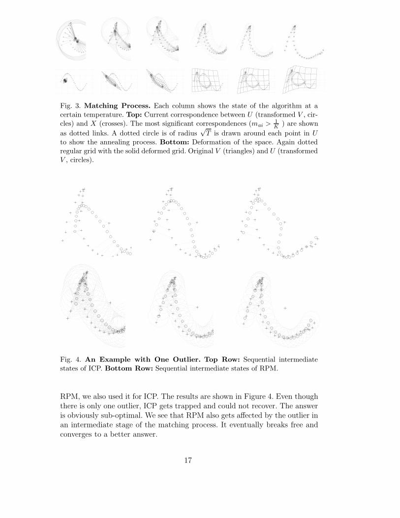
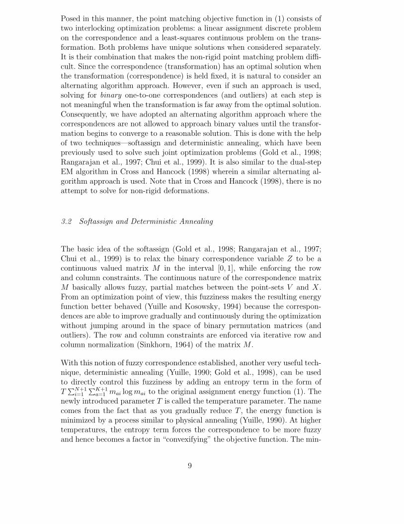
Fig. 3. Matching Process. Each column shows the state of the algorithm at acertain temperature. Top: Current correspondence between U (transformed V , cir-cles) and X (crosses). The most significant correspondences (mai >

1K

) are shown

as dotted links. A dotted circle is of radius√

T is drawn around each point in U

to show the annealing process. Bottom: Deformation of the space. Again dottedregular grid with the solid deformed grid. Original V (triangles) and U (transformedV , circles).

Fig. 4. An Example with One Outlier. Top Row: Sequential intermediatestates of ICP. Bottom Row: Sequential intermediate states of RPM.

RPM, we also used it for ICP. The results are shown in Figure 4. Even thoughthere is only one outlier, ICP gets trapped and could not recover. The answeris obviously sub-optimal. We see that RPM also gets affected by the outlier inan intermediate stage of the matching process. It eventually breaks free andconverges to a better answer.

17

5.2 Evaluation of RPM and ICP through Synthetic Examples

To test RPM’s performance, we ran a lot of experiments on synthetic data withdifferent degrees of warping, different amounts of noise and different amountsof outliers and compared it with ICP.

After a template point-set is chosen, we apply a randomly generated non-rigid transformation to warp it. Then we add noise or outliers to the warpedpoint-set to get a new target point-set. Instead of TPS, we use a differentnon-rigid mapping, namely Gaussian radial basis functions (RBF) (Yuille andGrzywacz, 1989) for the random transformation. The coefficients of the RBFwere sampled from a Gaussian distribution with a zero mean and a standarddeviation s1. Increasing the value of s1 generates more widely distributedRBF coefficients and hence leads to generally larger deformation. A certainpercentage of outliers and random noise are added to the warped templateto generate the target point-set. We then used both ICP and RPM to findthe best TPS to map the template set onto the target set. The errors arecomputed as the mean squared distance between the warped template usingthe TPS found by the algorithms and the warped template using the groundtruth Gaussian RBF.

We conducted three series of experiments. In the first series of experiments,the template was warped through progressively larger degrees of non-rigidwarpings. The warped templates were used as the target data without addingnoise or outliers. The purpose is to test the algorithms’ performance on solvingdifferent degrees of deformations. In the second series, different amounts ofGaussian noise (standard deviation s2 from 0 to 0.05) were added to thewarped template to get the target data. A medium degree of warping wasused to warp the template. The purpose is to test the algorithms’ toleranceof noise. In the third series, different amounts of random outliers (outlier tooriginal data ratio s3 ranging from 0 to 2) were added to the warped template.Again, a medium degree of warping was used. 100 random experiments wererepeated for each setting within each series.

We used two different templates. The first one comes from the outer contourof a tropical fish. The second one comes from a Chinese character (blessing),which is a more complex pattern. All three series of experiments were run onboth templates.

Some examples of these experiments are shown in Figures 5, 6, 7, 8, 9 and10. The final statistics (error means and standard deviations for each setting)are shown in Figure 11. ICP’s performance deteriorates much faster whenthe examples becomes harder due to any of these three factors—degree ofdeformation, amount of noise or amount of outliers. The difference is most

18

Fig. 5. Experiments on Deformation. Each column represent one example. Fromleft to right, increasing degree of deformation. Top Row: warped template. Second

Row: template and target(same as the warped template). Third Row: ICP results.Bottom Row: RPM results.

evident in the case of handling outliers. ICP starts failing in most of theexperiments and gives huge errors once outliers are added. On the other hand,RPM seems to be relatively unaffected. It is very interesting that this remainsthe case even when the numbers of outliers far exceeds the number of truedata points.

19

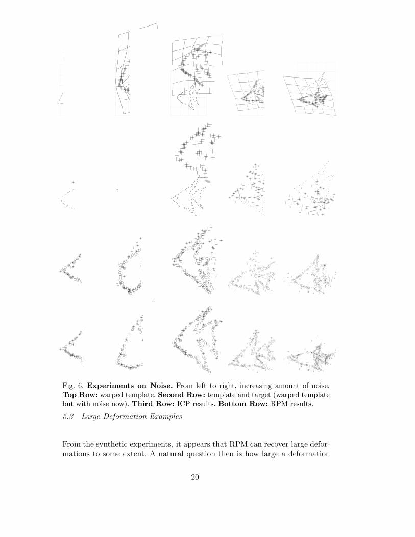
Fig. 6. Experiments on Noise. From left to right, increasing amount of noise.Top Row: warped template. Second Row: template and target (warped templatebut with noise now). Third Row: ICP results. Bottom Row: RPM results.

5.3 Large Deformation Examples

From the synthetic experiments, it appears that RPM can recover large defor-mations to some extent. A natural question then is how large a deformation

20

Fig. 7. Experiments on Outliers. From left to right, increasing amount of outliers.Top Row: warped template. Second Row: template and target (warped templatebut with outliers now). Third Row: ICP results. Bottom Row: RPM results.

21

Fig. 8. Experiments on Deformation. From left to right, increasing degree ofdeformation. Top Row: warped template. Second Row: template and target(sameas the warped template). Third Row: ICP results. Bottom Row: RPM results.

can RPM successfully recover. To answer this question, we conducted a newexperiment.

We hand-drew a sequence of 12 caterpillar images. The caterpillar is firstsupine. Then it gradually bends its tail toward its head. Further into thesequence, the bending increases. Points are extracted from each image in thesequence through thresholding. We then tried to match the first caterpillarpoint-set with the later deformed ones. The purpose is to test RPM’s abilityto track various degrees of deformation in the absence of outliers. The resultsof matching the first frame to the fifth, the seventh, the eleventh and thetwelfth frame are shown in Figure 12. We observed that up to frame eight,RPM is able to recover most of the desired transformation. Beyond that, it stilltries to warp the points to get the best fit and ends up generating “strange”unphysical warpings. This shows the limitation of the thin-plate spline. Wespeculate that a diffeomorphic mapping would be able to provide a bettersolution when combined with the correspondence engine in RPM.

22

Fig. 9. Experiments on Noise. From left to right, increasing amount of noise.Top Row: warped template. Second Row: template and target (warped templatebut with noise now). Third Row: ICP results. Bottom Row: RPM results.

5.4 Brain Mapping application

In brain mapping, one of the most important modules is a non-rigid anatom-ical brain MRI registration module. We now present preliminary experimentscomparing TPS-RPM with other techniques. We wish to point out at thisstage that we are merely trying to demonstrate the applicability of TPS-RPM to the non-rigid registration of cortical anatomical structures. Corticalsulci were traced using an SGI graphics platform (Rambo et al., 1998) with aray-casting technique that allows drawing in 3D space by projecting 2D coor-dinates of the tracing onto the exposed cortical surface. This is displayed onthe left in Figure 13. The inter-hemispheric fissure and 10 other major sulci

23

Fig. 10. Experiments on Outliers. From left to right, increasing amount of out-liers. Top Row: warped template. Second Row: template and target (warpedtemplate but with outliers now). Third Row: ICP results. Bottom Row: RPMresults.

(superior frontal, central, post-central, Sylvian and superior temporal on bothhemispheres) were extracted as point features. A sulcal point-set extractedfrom one subject is shown on the right in Figure 13. Since there is no guaran-tee of consistency of cortical sulci across subjects, we restricted ourselves tomajor sulci. Also, representing sulci as curves is essentially wrong since theyare three-dimensional ribbon-like structures. And the TPS in 3D is poorly con-strained by using 3D space curves as features. Despite these objections, we feelthat this example demonstrates an application of TPS-RPM to a real-worldproblem. We are currently working on a much more realistic brain mappingapplication using 3D ribbon representations for sulci (Chui et al., 2002).

The original sulcal point-sets normally contain around 3,000 points each. Thepoint-set is first sub-sampled to have around 300 points by taking every tenthpoint. The original MRI volume’s size is 106(X) x 75(Y) x 85(Z, slices). Withthat in mind, it is reasonable to assume that the average distances between

24

0 0.02 0.04 0.06 0.08 0.1−0.05

0

0.05

0.1

0.15

0.2

Degree of Deformation

Err

or

ICPRPM

−0.02 0 0.02 0.04 0.06−0.05

0

0.05

0.1

0.15

Noise Level

Err

or

ICPRPM

−1 0 1 2 3−0.05

0

0.05

0.1

0.15

0.2

0.25

Outlier to Data Ratio

Err

or ICPRPM

0 0.02 0.04 0.06 0.08 0.1−0.05

0

0.05

0.1

0.15

0.2

Degree of Deformation

Err

or

ICPRPM

−0.02 0 0.02 0.04 0.06−0.05

0

0.05

0.1

0.15

0.2

Noise LevelE

rror

ICPRPM

−1 0 1 2 3−0.05

0

0.05

0.1

0.15

0.2

Outlier to Data Ratio

Err

or

ICPRPM

Fig. 11. Statistics of the Synthetic Experiments. Top: Results using the fishtemplate. Bottom: Results using the Chinese character template. Note especiallyhow RPM’s errors increase much slower than ICP’s errors in all cases.

Fig. 12. Large Deformation—Caterpillar Example. From left to right, match-ing frame 1 to frame 5, 7, 11 and 12. Top: Original location. Middle: matchedresult. Bottom: deformation found.

points before registration should be in the range of 10-100. We set our startingtemperature to be roughly in the same range. After registration, we wouldexpect the average distance between corresponding points to be within a fewvoxels (say, 1-10). Our final temperature should be slightly smaller. From theseconsiderations, we set the RPM annealing parameters to be the following:Tinit = 50 , Tfinal = 1 , Tanneal−rate = 0.95. The regularization parameters arelinearly varied with the temperature as described above.

25

Fig. 13. Brain Mapping example. Left: The sulcal tracing tool with sometraced sulci on the 3D MR brain volume. Right: Sulci extracted and displayedas point-sets.

5.4.1 Sulcal Point Matching: A Comparison between Voxel-based matching(UMDS) and RPM

We applied TPS-RPM to five sulcal point-sets and compared it with threeother methods which use affine (and piecewise-affine) transformations for brainregistration.

We suspected that the voxel-based methods’ performance would not be assatisfying as feature-based methods for sulcal alignment. To test this, we com-pared RPM with a voxel-based affine mapping method (UMDS) (Studholme,1997) which maximizes the mutual information between the two volumes. Thevolumes were then matched using UMDS as described in (Studholme, 1997)and the resulting spatial mapping was applied to the sulcal points. RPM wasseparately run on the sulcal point-sets, and the results from global affine, piece-wise affine and thin-plate spline mappings are shown in Figures 14 and 15.Since we register every brain to the first one, after registration, the minimumdistance from each sulcal point in the current brain to the first is calculated.

The above comparison of RPM with the voxel-based UMDS approach showsthat RPM can improve upon a voxel-based approach at the sulci. The signifi-cant improvement from the global affine transformations by allowing piecewiseaffine and thin-plate spline mappings confirmed our belief in the importanceof non-rigid transformations. However, these results are clearly preliminarysince the errors were evaluated only at the sulci—exactly at the locationswhere a feature-based approach can be expected to perform best. Under nocircumstances should this preliminary result be seen as demonstrating any-thing of clinical significance. Much more detailed validation and evaluationexperiments comparing and contrasting voxel- and feature-based methods are

26

Fig. 14. Sulcal point mapping. The mapping results of five brains’ sulcalpoint-sets on the left side of the brain are shown together. Top Left: Voxel-basedmutual information with an affine mapping, Top Right: RPM with an affinemapping, Bottom Left: RPM with a piecewise affine mapping, Bottom Right:

TPS-RPM with a thin-plate spline mapping. Denser, closely packed distributions ofsulcal points suggest that they are better aligned. We clearly see the improvementof RPM over the voxel-based approach at the sulci. This is especially obvious forTPS-RPM.

required before any firm conclusions can be reached.

6 Discussion and Conclusions

There are two important free parameters in the new non-rigid point matchingalgorithm—the regularization parameter λ and the outlier rejection parameterζ. Below, we discuss ways of reducing the dependence on these free parameters.

Recall that the development of the TPS-RPM algorithm naturally lead to theregularization parameter value essentially being driven by the temperature.In the beginning, at high temperature, the regularization is very high and thealgorithm focuses on rigid mappings. At lower temperatures, the regulariza-tion is much lower and non-rigid deformations emerge. This is no accident.

27

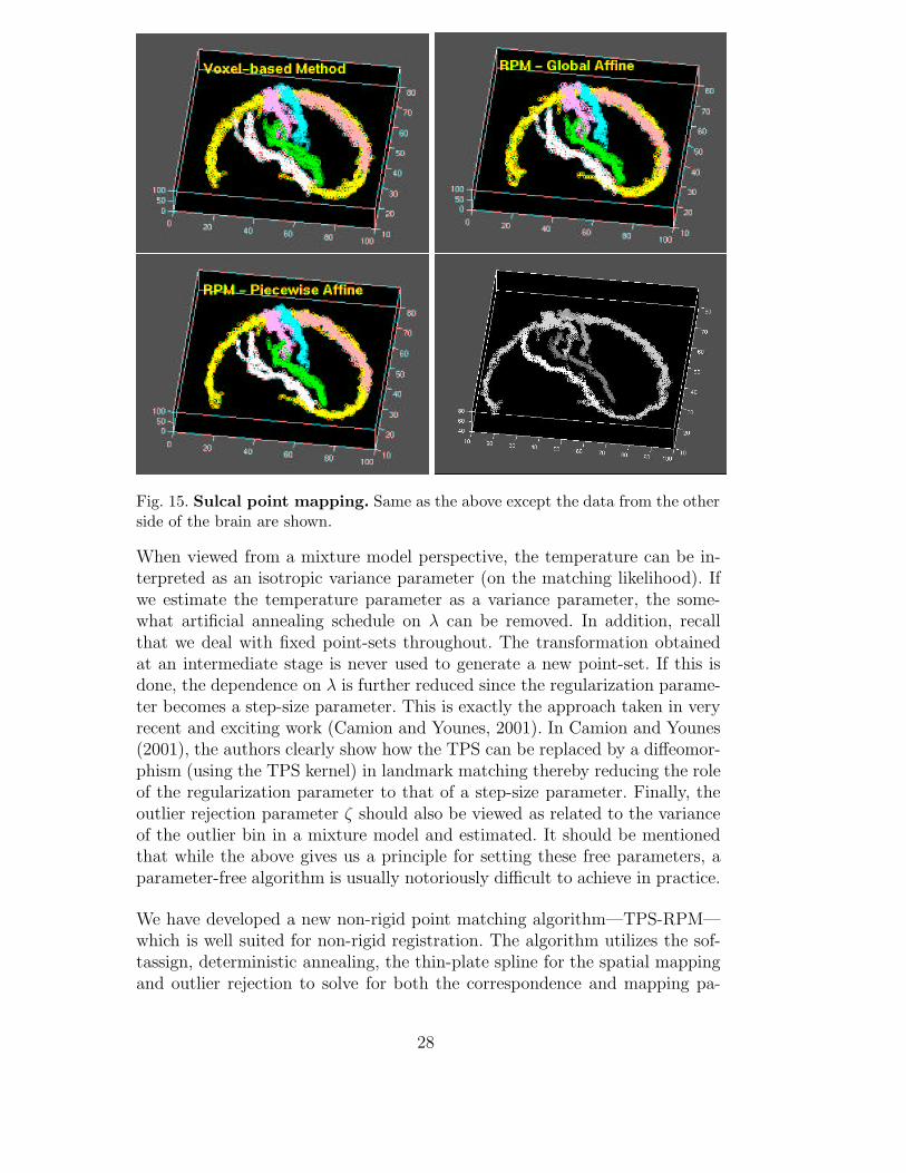
Fig. 15. Sulcal point mapping. Same as the above except the data from the otherside of the brain are shown.

When viewed from a mixture model perspective, the temperature can be in-terpreted as an isotropic variance parameter (on the matching likelihood). Ifwe estimate the temperature parameter as a variance parameter, the some-what artificial annealing schedule on λ can be removed. In addition, recallthat we deal with fixed point-sets throughout. The transformation obtainedat an intermediate stage is never used to generate a new point-set. If this isdone, the dependence on λ is further reduced since the regularization parame-ter becomes a step-size parameter. This is exactly the approach taken in veryrecent and exciting work (Camion and Younes, 2001). In Camion and Younes(2001), the authors clearly show how the TPS can be replaced by a diffeomor-phism (using the TPS kernel) in landmark matching thereby reducing the roleof the regularization parameter to that of a step-size parameter. Finally, theoutlier rejection parameter ζ should also be viewed as related to the varianceof the outlier bin in a mixture model and estimated. It should be mentionedthat while the above gives us a principle for setting these free parameters, aparameter-free algorithm is usually notoriously difficult to achieve in practice.

We have developed a new non-rigid point matching algorithm—TPS-RPM—which is well suited for non-rigid registration. The algorithm utilizes the sof-tassign, deterministic annealing, the thin-plate spline for the spatial mappingand outlier rejection to solve for both the correspondence and mapping pa-

28

rameters. The computational complexity of the algorithm is largely dependenton the implementation of the spline deformation [which can be O(N 3) in theworst case]. We have conducted carefully designed synthetic experiments toempirically demonstrate the superiority of the TPS-RPM algorithm over TPS-ICP and have also applied the algorithm to perform non-rigid registration ofcortical anatomical structures. While the algorithm is based on the notion ofone-to-one correspondence, it is possible to extend it to the case of many-to-many matching (Chui et al., 2002) which is the case in dense (as opposedto sparse) feature-based registration. We plan to further explore (Chui andRangarajan, 2001) the applicability of point matching-based approaches torelated problems in non-rigid registration such as anatomical atlases.

Acknowledgments

We acknowledge support from NSF IIS-0196457. We thank Larry Win, JimRambo, Bob Schultz and Jim Duncan for making available the sulcal dataused in the brain mapping experiments and Colin Studholme for providing uswith his implementation of UMDS.

A reference MATLAB���

implementation of TPS-RPM (with many of the 2Dexamples used here) is available under the terms of the GNU General Public li-cense (GPL) at http://www.cise.ufl.edu/˜anand/students/chui/rese-arch.html.

References

Amit, Y., Kong, A., 1996. Graphical templates for model recognition. IEEETrans. Patt. Anal. Mach. Intell. 18 (4), 225–236.

Baird, H., 1984. Model-based image matching using location. MIT Press, Cam-bridge, MA.

Ballard, D. H., 1981. Generalized Hough transform to detect arbitrary pat-terns. IEEE Trans. Patt. Anal. Mach. Intell. 13 (2), 111–122.

Belongie, S., Malik, J., Puzicha, J., 2002. Shape matching and object recog-nition using shape contexts. IEEE Trans. Patt. Anal. Mach. Intell. 24 (4),509–522.

Besl, P. J., McKay, N. D., 1992. A method for registration of 3-D shapes.IEEE Trans. Patt. Anal. Mach. Intell. 14 (2), 239–256.

Bhatia, R., 1996. Matrix analysis. Vol. 169 of Graduate Texts in Mathematics.Springer, New York, NY, page 38.

Bookstein, F. L., 1989. Principal warps: Thin-plate splines and the decomposi-tion of deformations. IEEE Trans. Patt. Anal. Mach. Intell. 11 (6), 567–585.

29

Camion, V., Younes, L., 2001. Geodesic interpolating splines. In: Energy Min-imization Methods for Computer Vision and Pattern Recognition (EMM-CVPR). Springer, New York, pp. 513–527.

Chui, H., Rambo, J., Duncan, J., Schultz, R., Rangarajan, A., 1999. Regis-tration of cortical anatomical structures via robust 3D point matching. In:Information Processing in Medical Imaging (IPMI). Springer, pp. 168–181.

Chui, H., Rangarajan, A., 2001. Learning an atlas from unlabeled point-sets.In: IEEE Workshop on Mathematical Methods in Biomedical Image Anal-ysis (MMBIA). IEEE Press, pp. 58–65.

Chui, H., Win, L., Duncan, J., Schultz, R., Rangarajan, A., 2002. A unifiednon-rigid feature registration method for brain mapping. Medical ImageAnalysis (in press).

Cootes, T., Taylor, C., Cooper, D., Graham, J., 1995. Active shape models:Their training and application. Computer Vision and Image Understanding61 (1), 38–59.

Cross, A. D. J., Hancock, E. R., 1998. Graph matching with a dual-step EMalgorithm. IEEE Trans. Patt. Anal. Mach. Intell. 20 (11), 1236–1253.

Feldmar, J., Ayache, N., May 1996. Rigid, affine and locally affine registrationof free-form surfaces. Intl. J. Computer Vision 18 (2), 99–119.

Geiger, D., Girosi, F., 1991. Parallel and deterministic algorithms from MRFs:Surface reconstruction. IEEE Trans. Patt. Anal. Mach. Intell. 13 (5), 401–412.

Gold, S., Rangarajan, A., 1996a. A graduated assignment algorithm for graphmatching. IEEE Trans. Patt. Anal. Mach. Intell. 18 (4), 377–388.

Gold, S., Rangarajan, A., 1996b. Softassign versus softmax: Benchmarks incombinatorial optimization. In: Touretzky, D. S., Mozer, M. C., Hasselmo,M. E. (Eds.), Advances in Neural Information Processing Systems (NIPS)8. MIT Press, Cambridge, MA, pp. 626–632.

Gold, S., Rangarajan, A., Lu, C. P., Pappu, S., Mjolsness, E., 1998. New algo-rithms for 2-D and 3-D point matching: pose estimation and correspondence.Pattern Recognition 31 (8), 1019–1031.

Grimson, E., 1990. Object recognition by computer: The role of geometricconstraints. MIT Press, Cambridge, MA.

Grimson, E., Lozano-Perez, T., 1987. Localizing overlapping parts by searchingthe interpretation tree. IEEE Trans. Patt. Anal. Mach. Intell. 9, 468–482.

Hibbard, L. S., Hawkins, R. A., 1988. Objective image alignment for three-dimensional reconstruction of digital autoradiograms. J. Neuroscience Meth-ods 26, 55–75.

Hinton, G., Williams, C., Revow, M., 1992. Adaptive elastic models for hand-printed character recognition. In: Moody, J., Hanson, S., Lippmann, R.(Eds.), Advances in Neural Information Processing Systems (NIPS) 4. Mor-gan Kaufmann, San Mateo, CA, pp. 512–519.

Hofmann, T., Buhmann, J. M., 1997. Pairwise data clustering by deterministicannealing. IEEE Trans. Patt. Anal. Mach. Intell. 19 (1), 1–14.

Hummel, R., Wolfson, H., 1988. Affine invariant matching. In: Proceedings of

30

the DARPA Image Understanding Workshop. Cambridge, MA, pp. 351–364.Huttenlocher, D. P., Klanderman, G. A., Rucklidge, W. J., 1993. Comparing

images using the Hausdorff distance. IEEE Trans. Patt. Anal. Mach. Intell.15 (9), 850–863.

Lamdan, Y., Schwartz, J., Wolfson, H., 1988. Object recognition by affineinvariant matching. IEEE Conf. Comp. Vision, Patt. Recog. , 335–344.

Lohmann, G., von Cramon, D. Y., 2000. Automatic labelling of the humancortical surface using sulcal basins. Medical Image Analysis 4 (3), 179–188.

Metaxas, D., Koh, E., Badler, N. I., 1997. Multi-level shape representationusing global deformations and locally adaptive finite elements. Intl. J. Com-puter Vision 25 (1), 49–61.

Papadimitriou, C., Steiglitz, K., 1982. Combinatorial optimization. Prentice-Hall, Inc., Englewood Cliffs, NJ.

Rambo, J., Zeng, X., Schultz, R., Win, L., Staib, L., Duncan, J., 1998. Plat-form for visualization and measurement of gray matter volume and surfacearea within discrete cortical regions from MR images. NeuroImage 7 (4),795.

Rangarajan, A., Chui, H., Bookstein, F., 1997. The softassign Procrustesmatching algorithm. In: Information Processing in Medical Imaging (IPMI).Springer, pp. 29–42.

Rohr, K., Stiehl, H., Sprengel, R., Buzug, T., Weese, J., Kuhn, M., 2001.Landmark-based elastic registration using approximating thin-plate splines.IEEE Trans. Med. Imag. 20, 526–534.

Sclaroff, S., Pentland, A. P., 1995. Modal matching for correspondence andrecognition. IEEE Trans. Patt. Anal. Mach. Intell. 17 (6), 545–561.

Scott, G., Longuet-Higgins, C., 1991. An algorithm for associating the featuresof two images. Proc. Royal Society of London B244, 21–26.

Shapiro, L., Brady, J., 1992. Feature-based correspondence: an eigenvectorapproach. Image and Vision Computing 10, 283–288.

Shapiro, L. G., Haralick, R. M., 1981. Structural descriptions and inexactmatching. IEEE Trans. Patt. Anal. Mach. Intell. 3 (9), 504–519.

Sinkhorn, R., 1964. A relationship between arbitrary positive matrices anddoubly stochastic matrices. Ann. Math. Statist. 35, 876–879.

Stockman, G., 1987. Object recognition and localization via pose clustering.Computer Vision, Graphics, and Image Processing 40 (3), 361–387.

Studholme, C., 1997. Measures of 3D medical image alignment. Ph.D. thesis,University of London, London, U.K.

Szeliski, R., Lavallee, S., 1996. Matching 3D anatomical surfaces with non-rigiddeformations using octree splines. Intl. J. Computer Vision 18, 171–186.

Tagare, H., O’Shea, D., Rangarajan, A., 1995. A geometric criterion forshape based non-rigid correspondence. In: Fifth Intl. Conf. Computer Vision(ICCV). pp. 434–439.

Ullman, S., 1989. Aligning pictorial descriptions: An approach to object recog-nition. Cognition 32 (3), 193–254.

Wahba, G., 1990. Spline models for observational data. SIAM, Philadelphia,

31

PA.Wells, W., 1997. Statistical approaches to feature-based object recognition.

Intl. J. Computer Vision 21 (1/2), 63–98.Yuille, A. L., 1990. Generalized deformable models, statistical physics, and

matching problems. Neural Computation 2 (1), 1–24.Yuille, A. L., Grzywacz, N. M., 1989. A mathematical analysis of the motion

coherence theory. Intl. J. Computer Vision 3 (2), 155–175.Yuille, A. L., Kosowsky, J. J., 1994. Statistical physics algorithms that con-

verge. Neural Computation 6 (3), 341–356.

32