a new method to determine the yield stress of a fluid from velocity profiles in a capillary

Available in: http://www.redalyc.org/articulo.oa?id=62028007012

Red de Revistas Científicas de América Latina, el Caribe, España y Portugal

Sistema de Información Científica

López-Durán, J.J.; Pérez-González, J.; Marín-Santibáñez, B.M.; Rodríguez-González, F.

A NEW METHOD TO DETERMINE THE YIELD STRESS OF A FLUID FROM VELOCITY PROFILES IN A

CAPILLARY

Revista Mexicana de Ingeniería Química, vol. 12, núm. 1, 2013, pp. 121-128

Universidad Autónoma Metropolitana Unidad Iztapalapa

Distrito Federal, México

How to cite Complete issue More information about this article Journal's homepage

Revista Mexicana de Ingeniería Química,

ISSN (Printed Version): 1665-2738

[email protected]

Universidad Autónoma Metropolitana Unidad

Iztapalapa

México

www.redalyc.orgNon-Profit Academic Project, developed under the Open Acces Initiative

http://www.redalyc.org

http://www.redalyc.org/comocitar.oa?id=62028007012

http://www.redalyc.org/fasciculo.oa?id=620&numero=28007

http://www.redalyc.org/articulo.oa?id=62028007012

http://www.redalyc.org/revista.oa?id=620

http://www.redalyc.org/articulo.oa?id=62028007012



http://www.redalyc.org


Revista Mexicana de Ingeniería Química

CONTENIDO

Volumen 8, número 3, 2009 / Volume 8, number 3, 2009

213 Derivation and application of the Stefan-Maxwell equations

(Desarrollo y aplicación de las ecuaciones de Stefan-Maxwell)

Stephen Whitaker

Biotecnología / Biotechnology

245 Modelado de la biodegradación en biorreactores de lodos de hidrocarburos totales del petróleo

intemperizados en suelos y sedimentos

(Biodegradation modeling of sludge bioreactors of total petroleum hydrocarbons weathering in soil

and sediments)

S.A. Medina-Moreno, S. Huerta-Ochoa, C.A. Lucho-Constantino, L. Aguilera-Vázquez, A. Jiménez-

González y M. Gutiérrez-Rojas

259 Crecimiento, sobrevivencia y adaptación de Bifidobacterium infantis a condiciones ácidas

(Growth, survival and adaptation of Bifidobacterium infantis to acidic conditions)

L. Mayorga-Reyes, P. Bustamante-Camilo, A. Gutiérrez-Nava, E. Barranco-Florido y A. Azaola-

Espinosa

265 Statistical approach to optimization of ethanol fermentation by Saccharomyces cerevisiae in the

presence of Valfor® zeolite NaA

(Optimización estadística de la fermentación etanólica de Saccharomyces cerevisiae en presencia de

zeolita Valfor® zeolite NaA)

G. Inei-Shizukawa, H. A. Velasco-Bedrán, G. F. Gutiérrez-López and H. Hernández-Sánchez

Ingeniería de procesos / Process engineering

271 Localización de una planta industrial: Revisión crítica y adecuación de los criterios empleados en

esta decisión

(Plant site selection: Critical review and adequation criteria used in this decision)

J.R. Medina, R.L. Romero y G.A. Pérez

Revista Mexicanade Ingenierıa Quımica

1

Academia Mexicana de Investigacion y Docencia en Ingenierıa Quımica, A.C.

Volumen 12, Numero 1, Abril 2013

ISSN 1665-2738

1Vol. 12, No. 1 (2013) 121-128

A NEW METHOD TO DETERMINE THE YIELD STRESS OF A FLUID FROMVELOCITY PROFILES IN A CAPILLARY

UN METODO NUEVO PARA DETERMINAR EL ESFUERZO DE CEDENCIA APARTIR DE LOS PERFILES DE VELOCIDAD EN UN CAPILAR

J.J. Lopez-Duran1, J. Perez-Gonzalez1∗, B.M. Marın-Santibanez2 and F. Rodrıguez-Gonzalez3

1Laboratorio de Reologıa, Escuela Superior de Fısica y Matematicas, Instituto Politecnico Nacional, U. P. AdolfoLopez Mateos Edif. 9, Col. San Pedro Zacatenco, C. P. 07738, Mexico D. F., Mexico

2Seccion de Estudios de Posgrado e Investigacion, Escuela Superior de Ingenierıa Quımica e IndustriasExtractivas, Instituto Politecnico Nacional, U. P. Adolfo Lopez Mateos Edif. 8,

Col. San Pedro Zacatenco, C. P. 07738, Mexico D. F., Mexico3Departamento de Biotecnologıa, Centro de Desarrollo de Productos Bioticos, Instituto Politecnico Nacional,

Col. San Isidro, C.P. 62731, Yautepec, Morelos, Mexico

Received 4 of September 2012; Accepted 13 of January 2013

AbstractA new method to determine the yield stress of a fluid from velocity profiles in capillary flow is presented in this work. Themethod is based on the calculation of the first derivative of the velocity profiles. For this, the velocity profiles of a model yieldstress fluid, 0.2 wt.% Carbopol gel, in a capillary were obtained by using a two dimensional particle image velocimetry system.It is shown that the yield stress value may be reliably determined by using only the velocity profiles and the measured wall shearstresses. This fact is corroborated by independent measurements of the yield stress with a stress controlled vane rheometer. Onthe other hand, the main details of the flow kinematics of yield-stress fluids were also registered and described in this work.Finally, it was found that the gel slips at the wall with a slip velocity that increases in a power-law way with the shear stress.

Keywords: yield stress, capillary rheometry, particle image velocimetry, Herschel-Bulkley model, wall slip.

ResumenEn este trabajo se presenta un nuevo metodo para determinar el esfuerzo de cedencia de un fluido a partir de sus perfiles develocidad en un capilar. El metodo se basa en el calculo de la primera derivada de los perfiles de velocidad. Para esto, seobtuvieron los perfiles de velocidad de un fluido modelo con esfuerzo de cedencia, 0.2 wt.% Carbopol gel, en un capilar pormedio de velocimetrıa por imagenes de partıculas. Se muestra que el esfuerzo de cedencia se puede determinar de maneraconfiable usando solamente los perfiles de velocidad y el esfuerzo cortante en la pared. Este hecho es corroborado mediantemediciones independientes del esfuerzo de cedencia con un reometro de paletas de esfuerzo controlado. Por otro lado, losprincipales detalles de la cinematica de flujo de fluidos con esfuerzo de cedencia fueron registrados y descritos en este trabajo.Finalmente, se encontro que el gel desliza en la pared del capilar con una velocidad que depende como una ley de potencia delesfuerzo cortante.

Palabras clave: esfuerzo de cedencia, reometrıa de capilar, velocimetrıa por imagenes de partıculas, modelo deHerschel-Bulkley, deslizamiento.

∗Corresponding author. E-mail: [email protected]./Fax 55-57-29-60-00, Ext. 55032

Publicado por la Academia Mexicana de Investigacion y Docencia en Ingenierıa Quımica A.C. 121

Lopez-Duran et al./ Revista Mexicana de Ingenierıa Quımica Vol. 12, No. 1 (2013) 121-128Lopez-Duran et al./ Revista Mexicana de Ingenierıa Quımica Vol. 12, No. 1 (2013) XXX-XXX

1 Introduction37

Yield-stress fluids are defined as materials that require38

the application of a critical shear stress (τy) to initiate39

the flow. Thus, such materials exhibit a solid-40

like behavior for shear stresses below τy and then41

flow for shear stresses above τy. In practice, a42

large amount of daily use products display this also43

called viscoplastic behavior, including foods, cleaning44

products, emulsions, pastes and concrete among many45

others.46

The existence of a yield stress has been a matter47

of debate for a long time, since its measured value48

depends on the experimental conditions, as sample49

preparation, as well as on the sensitivity of the50

rheometer utilized (Barnes and Walters, 1985; Nguyen51

and Boger, 1992; Barnes, 1999; Watson, 2004). From52

the practical point of view, however, the concept of53

yield stress has been widespread and has become very54

helpful in industry. For example, the yield stress is55

a useful parameter for the assessment of shelf-life of56

paints and other consuming products.57

The steady shear properties of yield-stress fluids58

have been measured mainly by using torsional59

rheometers. Provided that slip is restricted, a stress60

controlled rotational rheometer can give a relatively61

fast and meaningful value of the yield stress (Keentok,62

1982). On the contrary, pressure-driven rheometers,63

as the capillary one, do not have the acceptation64

of their torsional counterparts for yield-stress fluids65

characterization. The main reason for this is that66

experiments with capillaries are very time consuming67

and the results may be affected by slip at the capillary68

wall. In spite of this, capillary flow is present in many69

practical applications where the flow takes place at70

high shear rates, hence, a direct method to determine71

the conditions to initiate the flow, i.e., the yield stress,72

in this type of flow would be desirable.73

Magnin and Piau (1990) have stated that it is not74

possible to carry out rheometrical tests with yield-75

stress fluids without knowing the real kinematic field.76

However, as it happens with other rheological systems,77

most of the analysis of the flow of yield-stress fluids78

has been mainly done by rheometrical (mechanical)79

measurements, and the study of their kinematics in80

different geometries has received limited attention.81

Therefore, in the present work, a detailed analysis82

of the flow of a model yield-stress fluid, 0.2 wt.%83

Carbopol gel, in a capillary has been carried out by84

using particle image velocimetry (PIV) along with85

rheometrical measurements, which, to our knowledge,86

has not been made. PIV is a powerful non-invasive87

technique used to describe the flow kinematics in88

transparent fluids. Also, PIV is a whole-field method89

that allows for the determination of instantaneous90

velocity maps in a flow region. This last approach,91

of common use in fluid mechanics, has been gradually92

implemented for the analysis of the flow behavior of93

complex fluids (Perez-Gonzalez et al., 2012). Thus,94

by using PIV, we have been able to capture the main95

details of the flow development of a yield-stress fluid96

in the presence of slip at the wall. The results in97

this work show that the behavior of the fluid agrees98

well with the existence of a yield stress, which can be99

reliably determined from the velocity profiles and the100

measured wall shear stress.101

2 Theory102

Yield-stress fluids have been studied by theoretical103

and experimental methods and the main results are104

summarized in a series of reviews by different authors105

(see for example Cheng, 1986; Nguyen and Boger,106

1992; Denn and Bonn, 2011). The simplest yield-107

stress fluid, also known as the Bingham fluid, is108

described by the constitutive equation:109

τ = τy + ηpγ, τ > τy & γ = 0, τ ≤ τy (1)

where τ is the shear stress, τy is the yield stress; ηp is110

known as the plastic viscosity and γ is the shear rate.111

Eq. (1) predicts a Newtonian behavior once the fluid112

starts flowing. In practice, however, most fluids with a113

yield stress are shear-thinning. Thus, generalizations114

to account for the effect of shear-thinning have been115

introduced. A widespread model is the Hershel-116

Bulkley’s one, given by:117

τ = τy + kγn, τ > τy, & γ = 0, τ 6 τy (2)

Where k and n have the typical meaning of consistency118

and shear-thinning index, respectively.119

The characteristic flow curve of a yield-stress fluid120

contains a region of true flow preceded by another121

region without flow, but in which, slip may be present122

(Fig. 1). The transition between such regions, i. e., the123

yielding behavior, depends on whether slip is present124

or not (see for example Fig. 4 in Nguyen and Boger,125

1992). In the presence of slip in a capillary rheometer126

of given length (L) to diameter (D) ratio (L/D), the127

flow curve depends on the capillary diameter as well,128

and the transition between both regions is expected129

to be sharper for bigger diameters in shear-thinning130

fluids.131

2 www.rmiq.org

Lopez-Duran et al./ Revista Mexicana de Ingenierıa Quımica Vol. 12, No. 1 (2013) XXX-XXX

1 Introduction37

Yield-stress fluids are defined as materials that require38

the application of a critical shear stress (τy) to initiate39

the flow. Thus, such materials exhibit a solid-40

like behavior for shear stresses below τy and then41

flow for shear stresses above τy. In practice, a42

large amount of daily use products display this also43

called viscoplastic behavior, including foods, cleaning44

products, emulsions, pastes and concrete among many45

others.46

The existence of a yield stress has been a matter47

of debate for a long time, since its measured value48

depends on the experimental conditions, as sample49

preparation, as well as on the sensitivity of the50

rheometer utilized (Barnes and Walters, 1985; Nguyen51

and Boger, 1992; Barnes, 1999; Watson, 2004). From52

the practical point of view, however, the concept of53

yield stress has been widespread and has become very54

helpful in industry. For example, the yield stress is55

a useful parameter for the assessment of shelf-life of56

paints and other consuming products.57

The steady shear properties of yield-stress fluids58

have been measured mainly by using torsional59

rheometers. Provided that slip is restricted, a stress60

controlled rotational rheometer can give a relatively61

fast and meaningful value of the yield stress (Keentok,62

1982). On the contrary, pressure-driven rheometers,63

as the capillary one, do not have the acceptation64

of their torsional counterparts for yield-stress fluids65

characterization. The main reason for this is that66

experiments with capillaries are very time consuming67

and the results may be affected by slip at the capillary68

wall. In spite of this, capillary flow is present in many69

practical applications where the flow takes place at70

high shear rates, hence, a direct method to determine71

the conditions to initiate the flow, i.e., the yield stress,72

in this type of flow would be desirable.73

Magnin and Piau (1990) have stated that it is not74

possible to carry out rheometrical tests with yield-75

stress fluids without knowing the real kinematic field.76

However, as it happens with other rheological systems,77

most of the analysis of the flow of yield-stress fluids78

has been mainly done by rheometrical (mechanical)79

measurements, and the study of their kinematics in80

different geometries has received limited attention.81

Therefore, in the present work, a detailed analysis82

of the flow of a model yield-stress fluid, 0.2 wt.%83

Carbopol gel, in a capillary has been carried out by84

using particle image velocimetry (PIV) along with85

rheometrical measurements, which, to our knowledge,86

has not been made. PIV is a powerful non-invasive87

technique used to describe the flow kinematics in88

transparent fluids. Also, PIV is a whole-field method89

that allows for the determination of instantaneous90

velocity maps in a flow region. This last approach,91

of common use in fluid mechanics, has been gradually92

implemented for the analysis of the flow behavior of93

complex fluids (Perez-Gonzalez et al., 2012). Thus,94

by using PIV, we have been able to capture the main95

details of the flow development of a yield-stress fluid96

in the presence of slip at the wall. The results in97

this work show that the behavior of the fluid agrees98

well with the existence of a yield stress, which can be99

reliably determined from the velocity profiles and the100

measured wall shear stress.101

2 Theory102

Yield-stress fluids have been studied by theoretical103

and experimental methods and the main results are104

summarized in a series of reviews by different authors105

(see for example Cheng, 1986; Nguyen and Boger,106

1992; Denn and Bonn, 2011). The simplest yield-107

stress fluid, also known as the Bingham fluid, is108

described by the constitutive equation:109

τ = τy + ηpγ, τ > τy & γ = 0, τ ≤ τy (1)

where τ is the shear stress, τy is the yield stress; ηp is110

known as the plastic viscosity and γ is the shear rate.111

Eq. (1) predicts a Newtonian behavior once the fluid112

starts flowing. In practice, however, most fluids with a113

yield stress are shear-thinning. Thus, generalizations114

to account for the effect of shear-thinning have been115

introduced. A widespread model is the Hershel-116

Bulkley’s one, given by:117

τ = τy + kγn, τ > τy, & γ = 0, τ 6 τy (2)

Where k and n have the typical meaning of consistency118

and shear-thinning index, respectively.119

The characteristic flow curve of a yield-stress fluid120

contains a region of true flow preceded by another121

region without flow, but in which, slip may be present122

(Fig. 1). The transition between such regions, i. e., the123

yielding behavior, depends on whether slip is present124

or not (see for example Fig. 4 in Nguyen and Boger,125

1992). In the presence of slip in a capillary rheometer126

of given length (L) to diameter (D) ratio (L/D), the127

flow curve depends on the capillary diameter as well,128

and the transition between both regions is expected129

to be sharper for bigger diameters in shear-thinning130

fluids.131

2 www.rmiq.org122 www.rmiq.org


Figure 1. Schematic flow curve of a yield stress fluid. The dashed line represents the solid-

like behavior of the fluid, while the horizontal dotted line indicates the yield stress value.

132

Fig. 1. Schematic flow curve of a yield stress fluid.133

The vertical dashed line limits the solid-like behavior134

of the fluid, while the horizontal dotted line indicates135

the yield stress value.136

Thus, the yield stress may be determined by finding137

the critical shear stress at the transition between the138

two regions. The accuracy on the determination of139

such a value will depend on the sharpness of the140

transition as well as on the density of experimental141

points. Nevertheless, the yield stress, being a property142

of the material, should be independent of the capillary143

diameter.144

It is important to notice at this point that a145

single flow curve does not provide indication for the146

existence of a yield stress nor for the presence of147

slip. Moreover, the flow curve alone does not give148

information on the characteristics of the different flow149

regimes and additional information is required for150

a full description of the flow behavior of the fluid.151

Rodrıguez-Gonzalez et al. (2009) have shown that the152

calculation of the slip velocity and the whole analysis153

of the kinematics in capillary flow may be carried out,154

without using different capillary diameters, by means155

of the PIV technique. Thus, the velocity profiles may156

be used to calculate the yield stress of the fluid as157

shown below.158

The construction of the flow curves for capillary159

flow is based on the wall shear stress (τw) and the160

apparent shear rate (γapp) which are calculated as (Bird161

et al., 1977):162

τw =∆p(4 L

D

) (3)

163

γapp =32QπD3 (4)

Figure 2. a) Schematic velocity profile of a Herschel-Bulkley fluid and the shear stress

profile in a capillary. b) Derivative of the Herschel-Bulkley velocity profile with respect to

the radial position. Vertical dashed lines indicate the yielding position (r0) in the velocity

and shear rate profiles, respectively.

164

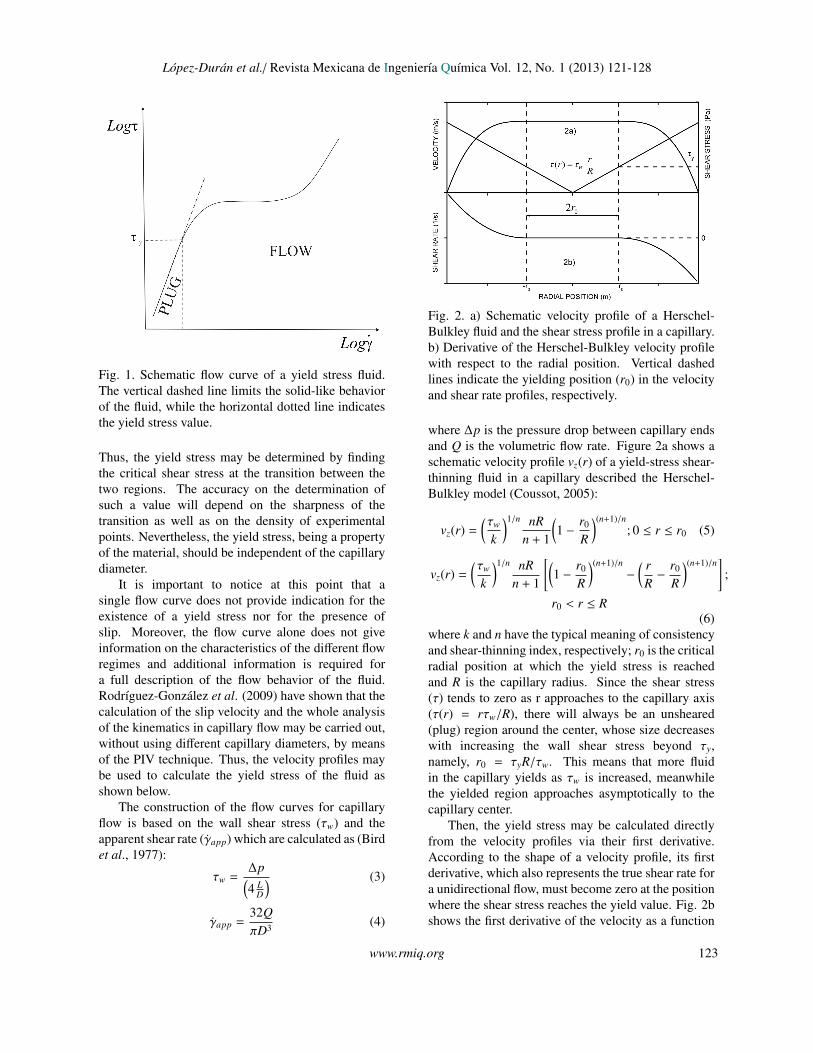
Fig. 2. a) Schematic velocity profile of a Herschel-165

Bulkley fluid and the shear stress profile in a capillary.166

b) Derivative of the Herschel-Bulkley velocity profile167

with respect to the radial position. Vertical dashed168

lines indicate the yielding position (r0) in the velocity169

and shear rate profiles, respectively.170

where ∆p is the pressure drop between capillary ends171

and Q is the volumetric flow rate. Figure 2a shows a172

schematic velocity profile vz(r) of a yield-stress shear-173

thinning fluid in a capillary described the Herschel-174

Bulkley model (Coussot, 2005):175

vz(r) =

(τw

k

)1/n nRn + 1

(1 − r0

R

)(n+1)/n; 0 ≤ r ≤ r0 (5)

176

vz(r) =

(τw

k

)1/n nRn + 1

[(1 − r0

R

)(n+1)/n−

( rR− r0

R

)(n+1)/n]

;

r0 < r ≤ R(6)

where k and n have the typical meaning of consistency177

and shear-thinning index, respectively; r0 is the critical178

radial position at which the yield stress is reached179

and R is the capillary radius. Since the shear stress180

(τ) tends to zero as r approaches to the capillary axis181

(τ(r) = rτw/R), there will always be an unsheared182

(plug) region around the center, whose size decreases183

with increasing the wall shear stress beyond τy,184

namely, r0 = τyR/τw. This means that more fluid185

in the capillary yields as τw is increased, meanwhile186

the yielded region approaches asymptotically to the187

capillary center.188

Then, the yield stress may be calculated directly189

from the velocity profiles via their first derivative.190

According to the shape of a velocity profile, its first191

derivative, which also represents the true shear rate for192

a unidirectional flow, must become zero at the position193

where the shear stress reaches the yield value. Fig. 2b194

shows the first derivative of the velocity as a function195

www.rmiq.org 3


Figure 1. Schematic flow curve of a yield stress fluid. The dashed line represents the solid-

like behavior of the fluid, while the horizontal dotted line indicates the yield stress value.

132

Fig. 1. Schematic flow curve of a yield stress fluid.133

The vertical dashed line limits the solid-like behavior134

of the fluid, while the horizontal dotted line indicates135

the yield stress value.136

Thus, the yield stress may be determined by finding137

the critical shear stress at the transition between the138

two regions. The accuracy on the determination of139

such a value will depend on the sharpness of the140

transition as well as on the density of experimental141

points. Nevertheless, the yield stress, being a property142

of the material, should be independent of the capillary143

diameter.144

It is important to notice at this point that a145

single flow curve does not provide indication for the146

existence of a yield stress nor for the presence of147

slip. Moreover, the flow curve alone does not give148

information on the characteristics of the different flow149

regimes and additional information is required for150

a full description of the flow behavior of the fluid.151

Rodrıguez-Gonzalez et al. (2009) have shown that the152

calculation of the slip velocity and the whole analysis153

of the kinematics in capillary flow may be carried out,154

without using different capillary diameters, by means155

of the PIV technique. Thus, the velocity profiles may156

be used to calculate the yield stress of the fluid as157

shown below.158

The construction of the flow curves for capillary159

flow is based on the wall shear stress (τw) and the160

apparent shear rate (γapp) which are calculated as (Bird161

et al., 1977):162

τw =∆p(4 L

D

) (3)

163

γapp =32QπD3 (4)

Figure 2. a) Schematic velocity profile of a Herschel-Bulkley fluid and the shear stress

profile in a capillary. b) Derivative of the Herschel-Bulkley velocity profile with respect to

the radial position. Vertical dashed lines indicate the yielding position (r0) in the velocity

and shear rate profiles, respectively.

164

Fig. 2. a) Schematic velocity profile of a Herschel-165

Bulkley fluid and the shear stress profile in a capillary.166

b) Derivative of the Herschel-Bulkley velocity profile167

with respect to the radial position. Vertical dashed168

lines indicate the yielding position (r0) in the velocity169

and shear rate profiles, respectively.170

where ∆p is the pressure drop between capillary ends171

and Q is the volumetric flow rate. Figure 2a shows a172

schematic velocity profile vz(r) of a yield-stress shear-173

thinning fluid in a capillary described the Herschel-174

Bulkley model (Coussot, 2005):175

vz(r) =

(τw

k

)1/n nRn + 1

(1 − r0

R

)(n+1)/n; 0 ≤ r ≤ r0 (5)

176

vz(r) =

(τw

k

)1/n nRn + 1

[(1 − r0

R

)(n+1)/n−

( rR− r0

R

)(n+1)/n]

;

r0 < r ≤ R(6)

where k and n have the typical meaning of consistency177

and shear-thinning index, respectively; r0 is the critical178

radial position at which the yield stress is reached179

and R is the capillary radius. Since the shear stress180

(τ) tends to zero as r approaches to the capillary axis181

(τ(r) = rτw/R), there will always be an unsheared182

(plug) region around the center, whose size decreases183

with increasing the wall shear stress beyond τy,184

namely, r0 = τyR/τw. This means that more fluid185

in the capillary yields as τw is increased, meanwhile186

the yielded region approaches asymptotically to the187

capillary center.188

Then, the yield stress may be calculated directly189

from the velocity profiles via their first derivative.190

According to the shape of a velocity profile, its first191

derivative, which also represents the true shear rate for192

a unidirectional flow, must become zero at the position193

where the shear stress reaches the yield value. Fig. 2b194

shows the first derivative of the velocity as a function195

www.rmiq.org 3www.rmiq.org 123


of the radial position (dv/dr) for the profile sketched196

in Fig. 2a. The position at which dv/dr = 0 in Fig. 2b197

is found as r0 and then, τy = r0τw/R.198

The numerical derivative of the velocity profiles199

with respect to the radial position may be calculated200

by a central difference approximation as shown below:201

(∂vz

∂r

)

i=

12

(vi+1 − vi

ri+i − ri+

vi − vi−1

ri − ri−1

)(7)

where vi indicates the local axial velocity at the ith202

radial position, ri, respectively (i = 1, . . . ,N, where N203

indicates the total points in the experimental velocity204

profile).205

3 Materials and methods206

The system studied here was a physical gel of207

Carbopol at a temperature of 25 ◦C. Carbopol is a208

polyacrylic acid that produces an acid solution when209

dispersed in water. Neutralization of the solution with210

a base results in a gel with plasticity and viscoelastic211

behavior (Piau, 2007). Neutralized gels made up of212

Carbopol are inexpensive, transparent and harmless213

materials with many applications, being the gel for214

hair one of the most popular. In addition, Carbopol215

gels have been used as model systems for the study of216

the flow behavior of viscoplastic materials.217

In order to make the gel, a solution was first218

prepared by dissolving 0.2 wt.% of Carbopol 940 (BF219

Goodrich) in tri-distilled water. Then, hollow glass220

spheres (as tracers for PIV) of 12 µm of average221

diameter (Sphericel 110 P8, Potters Industries), in222

a concentration of 0.2 wt.% were dispersed in the223

solution, which was further neutralized, according to224

the Carbopol content, with sodium hydroxide.225

Rheological measurements were performed in226

a pressure controlled capillary rheometer with a227

borosilicate glass capillary of L = 0.298 m and228

D =0.00294 m (L/D = 101.4). This large L/D229

ratio makes unnecessary pressure corrections for end230

effects. The reservoir from which the fluid was fed231

as well as the capillary were kept in a controlled232

temperature water bath at 25.0 ± 0.2 oC, but one part233

of the capillary remained out of the bath for PIV234

measurements. The pressure drop between capillary235

ends was measured with a Validyne R© differential236

pressure transducer and the flow rate was determined237

by collecting and measuring the ejected mass as a238

function of time. Only variations of around 1% in the239

flow rate were allowed for a given pressure condition240

to consider the flow as steady.241

Figure 3. Experimental set up. 1) Water bath, 2) glass capillary, 3) CCD camera, 4)

microscope, 5) Nd:YAG Laser, 6) Cylindrical lens, 7) prism, 8) biconvex lens, 9)

aberration corrector.

242

Fig. 3. Experimental set up. 1) Water bath, 2) glass243

capillary, 3) CCD camera, 4) microscope, 5) Nd:YAG244

Laser, 6) Cylindrical lens, 7) prism, 8) biconvex lens,245

9) aberration corrector.246

On the other hand, a stress controlled Paar Physica247

UDS 200 rotational rheometer with the FL 100 vane248

geometry was also utilized as an independent way to249

measure the yield stress.250

The study of the flow kinematics in the capillary251

was performed with a two dimensional PIV Dantec252

Dynamics system as sketched in Fig. 3. This system253

has been previously used for the analysis of the flow254

kinematics of micellar solutions (Marın-Santibanez et255

al., 2006) and polymer melts (Rodriguez-Gonzalez et256

al., 2009, 2010, 2011) in capillaries. All the details of257

the PIV set up to analyze capillary flow may be found258

elsewhere and only a brief description is presented259

here.260

The PIV system consists of a high speed and high261

sensitivity HiSense MKII CCD camera of 1.35 Mega-262

pixels, two coupled Nd:YAG lasers of 50 mJ with263

λ = 532 nm and the Dantec Dynamic Studio 2.1264

software. A light sheet was reduced in thickness up265

to less than 200 µm by using a biconvex lens with 0.05266

m of focal distance, and sent through the center plane267

of the capillary. An InfiniVar R© continuously-focusable268

video microscope CFM-2/S was attached to the CCD269

camera in order to increase the spatial resolution.270

The images taken by the PIV system covered an271

area of 0.00294 m × 0.00231 m which was located272

around an axial position of z = 75D downstream273

from the contraction. Series of fifty image pairs were274

obtained for each flow condition once the steady state275

was reached, and all the image pairs were correlated276

to obtain the corresponding velocity map. Then, the277

fifty velocity maps were averaged in time to obtain a278

single one, from which, the velocity as a function of279

the radial position (velocity profile) was obtained for280

the desired axial position.281

4 www.rmiq.org


of the radial position (dv/dr) for the profile sketched196

in Fig. 2a. The position at which dv/dr = 0 in Fig. 2b197

is found as r0 and then, τy = r0τw/R.198

The numerical derivative of the velocity profiles199

with respect to the radial position may be calculated200

by a central difference approximation as shown below:201

(∂vz

∂r

)

i=

12

(vi+1 − vi

ri+i − ri+

vi − vi−1

ri − ri−1

)(7)

where vi indicates the local axial velocity at the ith202

radial position, ri, respectively (i = 1, . . . ,N, where N203

indicates the total points in the experimental velocity204

profile).205

3 Materials and methods206

The system studied here was a physical gel of207

Carbopol at a temperature of 25 ◦C. Carbopol is a208

polyacrylic acid that produces an acid solution when209

dispersed in water. Neutralization of the solution with210

a base results in a gel with plasticity and viscoelastic211

behavior (Piau, 2007). Neutralized gels made up of212

Carbopol are inexpensive, transparent and harmless213

materials with many applications, being the gel for214

hair one of the most popular. In addition, Carbopol215

gels have been used as model systems for the study of216

the flow behavior of viscoplastic materials.217

In order to make the gel, a solution was first218

prepared by dissolving 0.2 wt.% of Carbopol 940 (BF219

Goodrich) in tri-distilled water. Then, hollow glass220

spheres (as tracers for PIV) of 12 µm of average221

diameter (Sphericel 110 P8, Potters Industries), in222

a concentration of 0.2 wt.% were dispersed in the223

solution, which was further neutralized, according to224

the Carbopol content, with sodium hydroxide.225

Rheological measurements were performed in226

a pressure controlled capillary rheometer with a227

borosilicate glass capillary of L = 0.298 m and228

D =0.00294 m (L/D = 101.4). This large L/D229

ratio makes unnecessary pressure corrections for end230

effects. The reservoir from which the fluid was fed231

as well as the capillary were kept in a controlled232

temperature water bath at 25.0 ± 0.2 oC, but one part233

of the capillary remained out of the bath for PIV234

measurements. The pressure drop between capillary235

ends was measured with a Validyne R© differential236

pressure transducer and the flow rate was determined237

by collecting and measuring the ejected mass as a238

function of time. Only variations of around 1% in the239

flow rate were allowed for a given pressure condition240

to consider the flow as steady.241

Figure 3. Experimental set up. 1) Water bath, 2) glass capillary, 3) CCD camera, 4)

microscope, 5) Nd:YAG Laser, 6) Cylindrical lens, 7) prism, 8) biconvex lens, 9)

aberration corrector.

242

Fig. 3. Experimental set up. 1) Water bath, 2) glass243

capillary, 3) CCD camera, 4) microscope, 5) Nd:YAG244

Laser, 6) Cylindrical lens, 7) prism, 8) biconvex lens,245

9) aberration corrector.246

On the other hand, a stress controlled Paar Physica247

UDS 200 rotational rheometer with the FL 100 vane248

geometry was also utilized as an independent way to249

measure the yield stress.250

The study of the flow kinematics in the capillary251

was performed with a two dimensional PIV Dantec252

Dynamics system as sketched in Fig. 3. This system253

has been previously used for the analysis of the flow254

kinematics of micellar solutions (Marın-Santibanez et255

al., 2006) and polymer melts (Rodriguez-Gonzalez et256

al., 2009, 2010, 2011) in capillaries. All the details of257

the PIV set up to analyze capillary flow may be found258

elsewhere and only a brief description is presented259

here.260

The PIV system consists of a high speed and high261

sensitivity HiSense MKII CCD camera of 1.35 Mega-262

pixels, two coupled Nd:YAG lasers of 50 mJ with263

λ = 532 nm and the Dantec Dynamic Studio 2.1264

software. A light sheet was reduced in thickness up265

to less than 200 µm by using a biconvex lens with 0.05266

m of focal distance, and sent through the center plane267

of the capillary. An InfiniVar R© continuously-focusable268

video microscope CFM-2/S was attached to the CCD269

camera in order to increase the spatial resolution.270

The images taken by the PIV system covered an271

area of 0.00294 m × 0.00231 m which was located272

around an axial position of z = 75D downstream273

from the contraction. Series of fifty image pairs were274

obtained for each flow condition once the steady state275

was reached, and all the image pairs were correlated276

to obtain the corresponding velocity map. Then, the277

fifty velocity maps were averaged in time to obtain a278

single one, from which, the velocity as a function of279

the radial position (velocity profile) was obtained for280

the desired axial position.281



4 Results and discussion282

4.1 Capillary rheometry283

Figure 4 shows the capillary flow curve for the gel284

(filled symbols), along with the one obtained from the285

integration of the velocity profiles (hollow symbols)286

according to:287

Q =

2π∫

0

R∫

0

rvz(r)drdθ (8)

Validation of the PIV measurements is performed by288

their direct comparison with rheometrical data in the289

flow curve. In this case, the data obtained from the290

velocity profiles agree well with the rheometrical ones;291

the maximum difference in the volumetric flow rates292

obtained by using the two methods was 6.5%, which293

shows the reliability of the PIV technique to describe294

the behavior of the gel in capillary flow.295

The flow curve covers a volumetric flow rate range296

from 10−8 to 10−6 m3/s (corresponding to an apparent297

shear rate range of about 300 s−1), and has been298

divided into two regions (I and II). Region I appears299

linear in the log-log plot and has, therefore, been fitted300

by a power-law equation (see the equations inserted in301

Fig. 4). The other region (II) contains a fairly smooth302

transition linked to straight line.303

Figure 4. Wall shear stress vs. volumetric flow rate for the Carbopol gel. Open and filled

symbols correspond to rheometrical and PIV measurements, respectively. The flow curve

was divided into two regions: (I) solid-like behavior (pure slip) and (II) flow with slip. The

continuous and dashed lines represent the fitting to models.

304

Fig. 4. Wall shear stress vs. volumetric flow rate for305

the Carbopol gel. Open and filled symbols correspond306

to rheometrical and PIV measurements, respectively.307

The flow curve was divided into two regions: (I) solid-308

like behavior (pure slip) and (II) flow with slip. The309

continuous and dashed lines represent the fitting to310

models.311

a)

312

b)

313

c)

Figure 5. Velocity profiles for different wall shear stresses for the Carbopol gel. a) 11.8 Pa,

18.1 Pa and 26.8 Pa; b) 27.2 Pa, 29.7 Pa and 33.2 Pa; c) 42.2 Pa, 54.2 Pa, 64.2 Pa and 71.6

Pa.

314

Fig. 5. Velocity profiles for different wall shear stresses315

for the Carbopol gel. a) 11.8 Pa, 18 Pa and 26.8 Pa; b)316

27.2 Pa, 29.7 Pa and 33.2 Pa; c) 42.2 Pa, 54.2 Pa, 64.2317

Pa and 71.6 Pa.318

The volumetric flow rate limiting regions I and II was319

established as that at the intersection of the straight320

line in region I with the curve in region II.321

www.rmiq.org 5


4 Results and discussion282

4.1 Capillary rheometry283

Figure 4 shows the capillary flow curve for the gel284

(filled symbols), along with the one obtained from the285

integration of the velocity profiles (hollow symbols)286

according to:287

Q =

2π∫

0

R∫

0

rvz(r)drdθ (8)

Validation of the PIV measurements is performed by288

their direct comparison with rheometrical data in the289

flow curve. In this case, the data obtained from the290

velocity profiles agree well with the rheometrical ones;291

the maximum difference in the volumetric flow rates292

obtained by using the two methods was 6.5%, which293

shows the reliability of the PIV technique to describe294

the behavior of the gel in capillary flow.295

The flow curve covers a volumetric flow rate range296

from 10−8 to 10−6 m3/s (corresponding to an apparent297

shear rate range of about 300 s−1), and has been298

divided into two regions (I and II). Region I appears299

linear in the log-log plot and has, therefore, been fitted300

by a power-law equation (see the equations inserted in301

Fig. 4). The other region (II) contains a fairly smooth302

transition linked to straight line.303

Figure 4. Wall shear stress vs. volumetric flow rate for the Carbopol gel. Open and filled

symbols correspond to rheometrical and PIV measurements, respectively. The flow curve

was divided into two regions: (I) solid-like behavior (pure slip) and (II) flow with slip. The

continuous and dashed lines represent the fitting to models.

304

Fig. 4. Wall shear stress vs. volumetric flow rate for305

the Carbopol gel. Open and filled symbols correspond306

to rheometrical and PIV measurements, respectively.307

The flow curve was divided into two regions: (I) solid-308

like behavior (pure slip) and (II) flow with slip. The309

continuous and dashed lines represent the fitting to310

models.311

a)

312

b)

313

c)

Figure 5. Velocity profiles for different wall shear stresses for the Carbopol gel. a) 11.8 Pa,

18.1 Pa and 26.8 Pa; b) 27.2 Pa, 29.7 Pa and 33.2 Pa; c) 42.2 Pa, 54.2 Pa, 64.2 Pa and 71.6

Pa.

314

Fig. 5. Velocity profiles for different wall shear stresses315

for the Carbopol gel. a) 11.8 Pa, 18 Pa and 26.8 Pa; b)316

27.2 Pa, 29.7 Pa and 33.2 Pa; c) 42.2 Pa, 54.2 Pa, 64.2317

Pa and 71.6 Pa.318

The volumetric flow rate limiting regions I and II was319

established as that at the intersection of the straight320

line in region I with the curve in region II.321



Figure 6. Slip velocity vs. wall shear stress for the Carbopol gel. The continuous line

represents the fitting to a power-law model.

322

Fig. 6. Slip velocity vs. wall shear stress for the323

Carbopol gel. The continuous line represents the324

fitting to a power-law model.325

4.2 Description of the flow kinematics326

Figures 5a-c show the velocity profiles for the different327

flow conditions investigated in this work, which328

clearly exhibit the changes in the velocity field with329

increasing the wall shear stress, namely, the profiles330

change from completely plug-like to shear-thinning331

like with a non-yielded region and slip at the wall. The332

average of the standard deviations for each profile was333

around 1%, which is of the size of the symbols used to334

represent the data. On the other hand, an analysis of335

the velocity maps (they are not shown here for the sake336

of space) shows that the velocity in the radial direction337

was at least three orders of magnitude smaller than338

the axial one in each case. Thus, the velocity profiles339

in Figs. 5a-c represent a unidirectional flow and the340

velocity field is simply given by vz = vz(r) for the341

different shear stresses, as it is expected for a fully342

developed shear flow.343

Figure 5a shows that for shear stresses in region I344

(below the yield value), the velocity profiles appear345

completely flat or plug-like, which is characteristic346

of a solid-like behavior. Then, region I in the flow347

curve may be attributed to plug flow. Under these348

conditions, the flow rate is only due to slip of the349

gel at the capillary wall. At the shear stress of 26.8350

Pa, it is possible to appreciate a slight development351

of flow near the capillary wall (see the highest profile352

in Fig. 5a), even though the velocity profile appears353

almost flat. Thus, this shear stress value, which is the354

first experimental point taken in region II, cannot be355

considered as corresponding to the yield stress, since356

Figure 7. First derivative of the velocity as a function of the radial position for the profile

obtained at τw= 64.2 Pa. Vertical dashed lines indicate the position at which dv/dr=0 (r0 =

0.000463±0.000032 m), which corresponds to τy = 20.2±1.4 Pa.

357

Fig. 7. First derivative of the velocity as a function358

of the radial position for the profile obtained at τw =359

64.2 Pa. Vertical dashed lines indicate the position at360

which dv/dr = 0 (r0 = 0.000463±0.000032 m), which361

corresponds to τy = 20.2±1.4 Pa.362

it already includes a flow development. Consequently,363

an accurate determination of the yield stress by using364

the pure rheometrical data require of a large number of365

experimental points, which would be very impractical.366

One way to face this problem is discussed in the next367

section.368

Beyond the yield stress, the velocity profiles in369

Figs. 5b-c show the plug-like region around the370

capillary axis and shear-thinning, both characteristic371

of a yield-stress fluid. In addition, the velocity profiles372

clearly exhibit a non-zero velocity at the wall, i. e., the373

gel slips at the capillary wall with a velocity (vs) that374

increases along with the wall shear stress (Fig. 6).375

4.3 Determination of the yield stress from376

velocity profiles377

As discussed in the previous section, an accurate378

determination of the yield stress by using the pure379

rheometrical data would require of a large number380

of experimental points, which would be impractical.381

This problem can be overcome by calculating the yield382

stress directly from the velocity profiles via their first383

derivative. For this, the true shear rate must be zero384

at the position where the shear stress reaches the yield385

value. Meanwhile, the corresponding shear stress is386

given by τ(r) = rτw/R. Figure 7 shows the first387

derivative of the velocity as a function of the radial388

position (dv/dr) for the profile obtained at τw = 64.2389

Pa. The position at which dv/dr = 0 in Fig. 7 is found390

as r0 = 0.000463 ± 0.000032 m, which corresponds391

to a shear stress value of 20.2 ± 1.4 Pa. If the same392

analysis is performed with all the velocity profiles in393

6 www.rmiq.org


Figure 6. Slip velocity vs. wall shear stress for the Carbopol gel. The continuous line

represents the fitting to a power-law model.

322

Fig. 6. Slip velocity vs. wall shear stress for the323

Carbopol gel. The continuous line represents the324

fitting to a power-law model.325

4.2 Description of the flow kinematics326

Figures 5a-c show the velocity profiles for the different327

flow conditions investigated in this work, which328

clearly exhibit the changes in the velocity field with329

increasing the wall shear stress, namely, the profiles330

change from completely plug-like to shear-thinning331

like with a non-yielded region and slip at the wall. The332

average of the standard deviations for each profile was333

around 1%, which is of the size of the symbols used to334

represent the data. On the other hand, an analysis of335

the velocity maps (they are not shown here for the sake336

of space) shows that the velocity in the radial direction337

was at least three orders of magnitude smaller than338

the axial one in each case. Thus, the velocity profiles339

in Figs. 5a-c represent a unidirectional flow and the340

velocity field is simply given by vz = vz(r) for the341

different shear stresses, as it is expected for a fully342

developed shear flow.343

Figure 5a shows that for shear stresses in region I344

(below the yield value), the velocity profiles appear345

completely flat or plug-like, which is characteristic346

of a solid-like behavior. Then, region I in the flow347

curve may be attributed to plug flow. Under these348

conditions, the flow rate is only due to slip of the349

gel at the capillary wall. At the shear stress of 26.8350

Pa, it is possible to appreciate a slight development351

of flow near the capillary wall (see the highest profile352

in Fig. 5a), even though the velocity profile appears353

almost flat. Thus, this shear stress value, which is the354

first experimental point taken in region II, cannot be355

considered as corresponding to the yield stress, since356

Figure 7. First derivative of the velocity as a function of the radial position for the profile

obtained at τw= 64.2 Pa. Vertical dashed lines indicate the position at which dv/dr=0 (r0 =

0.000463±0.000032 m), which corresponds to τy = 20.2±1.4 Pa.

357

Fig. 7. First derivative of the velocity as a function358

of the radial position for the profile obtained at τw =359

64.2 Pa. Vertical dashed lines indicate the position at360

which dv/dr = 0 (r0 = 0.000463±0.000032 m), which361

corresponds to τy = 20.2±1.4 Pa.362

it already includes a flow development. Consequently,363

an accurate determination of the yield stress by using364

the pure rheometrical data require of a large number of365

experimental points, which would be very impractical.366

One way to face this problem is discussed in the next367

section.368

Beyond the yield stress, the velocity profiles in369

Figs. 5b-c show the plug-like region around the370

capillary axis and shear-thinning, both characteristic371

of a yield-stress fluid. In addition, the velocity profiles372

clearly exhibit a non-zero velocity at the wall, i. e., the373

gel slips at the capillary wall with a velocity (vs) that374

increases along with the wall shear stress (Fig. 6).375


velocity profiles377

As discussed in the previous section, an accurate378

determination of the yield stress by using the pure379

rheometrical data would require of a large number380

of experimental points, which would be impractical.381

This problem can be overcome by calculating the yield382

stress directly from the velocity profiles via their first383

derivative. For this, the true shear rate must be zero384

at the position where the shear stress reaches the yield385

value. Meanwhile, the corresponding shear stress is386

given by τ(r) = rτw/R. Figure 7 shows the first387

derivative of the velocity as a function of the radial388

position (dv/dr) for the profile obtained at τw = 64.2389

Pa. The position at which dv/dr = 0 in Fig. 7 is found390

as r0 = 0.000463 ± 0.000032 m, which corresponds391

to a shear stress value of 20.2 ± 1.4 Pa. If the same392

analysis is performed with all the velocity profiles in393



Figure 8. Shear stress vs. shear strain for the Carbopol gel. The continuous line represents

the fitting to the Hooke model.

394

Fig. 8. Shear stress vs. shear strain for the Carbopol395

gel. The continuous line represents the fitting to the396

Hooke model.397

figs. 5b-c, considering the symmetry of the profiles (i.398

e., the values obtained at both sides of the profiles), an399

average value of 20.5 ± 1.2 Pa is obtained.400

Once the yielding position and the yield stress401

are determined, they can be inserted in Eqs. (5) and402

(6) to calculate the velocity profiles. Note that the403

experimental velocity profiles in Figs. 5a-c are very404

well described by the Herschel-Bulkley model (Eqs.405

5-6) with k = 3.679 Pa s0.5 and n = 0.5, which gives406

further support to the reliability of the yield stress407

calculated from the velocity profiles.408


vane rheometry410

Figure 8 shows the results of an analysis of the gel by411

a slow shear stress ramp in the vane rheometer. In this412

case, we have made use of the fact that for a solid-413

like behavior the relationship between the shear stress414

and shear deformation (γ) should be linear (Hookean415

behavior). It may be observed that the torque changes416

linearly with γ up to a value of 0.07, and then417

deviates from the linearity. The first experimental418

point considered as lying out of the straight line had419

a deviation of 6.3% in the torque value. The previous420

experimental point, which had a deviation of only421

4.75% with respect to the solid-like behavior, was used422

to calculate the yield stress for the gel as 20.6±0.9 Pa,423

which is in very good agreement with the yield stress424

value obtained from the velocity profiles.425

Summarizing, the yield stress values obtained426

from the different analysis are in good agreement,427

which shows that the new method presented here,428

based on the first derivative of the velocity profiles,429

is reliable and may be used for other fluids, provided430

that the velocity profiles are available.431

Conclusions432

The yielding and flow behavior of a model yield-433

stress fluid, 0.2 wt.% Carbopol gel, in a capillary with434

slip at the wall was investigated in this work by PIV.435

The flow behavior consists in a purely plug-like flow436

before yielding, followed by shear thinning with slip at437

relatively high shear rates. The velocity profiles were438

well described by the Herschel-Bulkley model and439

allowed for a reliably determination of the yield stress.440

The method presented here may be used for other441

fluids, provided that the velocity profiles are available.442

Finally, the slip velocity was found to increase in a443

power-law way with the shear stress.444

Acknowledgements445

This research was supported by SIP-IPN (No. Reg.446

20131369). J J. L.-D. had a PFI-IPN scholarship to447

perform this work and J. P.-G, B. M. M.-S and F. R-G448

are COFAA-EDI fellows.449

Nomenclature450

L length of the capillaryD diameter of the capillaryR radius of the capillaryr radial positionr0 radial position at which the yield

stress is reachedz axial positionvz axial velocity∆p pressure dropQ volumetric flow ratek consistency indexn shear-thinning index

451

Greek symbolsτ shear stressτw wall shear stressτy yield stressγ shear strainγ shear rateγapp apparent shear rateγr shear rate at a certain radial

positionγR shear rate at r = Rη shear viscosityηp plastic viscosity

452

www.rmiq.org 7


Figure 8. Shear stress vs. shear strain for the Carbopol gel. The continuous line represents

the fitting to the Hooke model.

394

Fig. 8. Shear stress vs. shear strain for the Carbopol395

gel. The continuous line represents the fitting to the396

Hooke model.397

figs. 5b-c, considering the symmetry of the profiles (i.398

e., the values obtained at both sides of the profiles), an399

average value of 20.5 ± 1.2 Pa is obtained.400

Once the yielding position and the yield stress401

are determined, they can be inserted in Eqs. (5) and402

(6) to calculate the velocity profiles. Note that the403

experimental velocity profiles in Figs. 5a-c are very404

well described by the Herschel-Bulkley model (Eqs.405

5-6) with k = 3.679 Pa s0.5 and n = 0.5, which gives406

further support to the reliability of the yield stress407

calculated from the velocity profiles.408


vane rheometry410

Figure 8 shows the results of an analysis of the gel by411

a slow shear stress ramp in the vane rheometer. In this412

case, we have made use of the fact that for a solid-413

like behavior the relationship between the shear stress414

and shear deformation (γ) should be linear (Hookean415

behavior). It may be observed that the torque changes416

linearly with γ up to a value of 0.07, and then417

deviates from the linearity. The first experimental418

point considered as lying out of the straight line had419

a deviation of 6.3% in the torque value. The previous420

experimental point, which had a deviation of only421

4.75% with respect to the solid-like behavior, was used422

to calculate the yield stress for the gel as 20.6±0.9 Pa,423

which is in very good agreement with the yield stress424

value obtained from the velocity profiles.425

Summarizing, the yield stress values obtained426

from the different analysis are in good agreement,427

which shows that the new method presented here,428

based on the first derivative of the velocity profiles,429

is reliable and may be used for other fluids, provided430

that the velocity profiles are available.431

Conclusions432

The yielding and flow behavior of a model yield-433

stress fluid, 0.2 wt.% Carbopol gel, in a capillary with434

slip at the wall was investigated in this work by PIV.435

The flow behavior consists in a purely plug-like flow436

before yielding, followed by shear thinning with slip at437

relatively high shear rates. The velocity profiles were438

well described by the Herschel-Bulkley model and439

allowed for a reliably determination of the yield stress.440

The method presented here may be used for other441

fluids, provided that the velocity profiles are available.442

Finally, the slip velocity was found to increase in a443

power-law way with the shear stress.444

Acknowledgements445

This research was supported by SIP-IPN (No. Reg.446

20131369). J J. L.-D. had a PFI-IPN scholarship to447

perform this work and J. P.-G, B. M. M.-S and F. R-G448

are COFAA-EDI fellows.449

Nomenclature450

L length of the capillaryD diameter of the capillaryR radius of the capillaryr radial positionr0 radial position at which the yield

stress is reachedz axial positionvz axial velocity∆p pressure dropQ volumetric flow ratek consistency indexn shear-thinning index

451

Greek symbolsτ shear stressτw wall shear stressτy yield stressγ shear strainγ shear rateγapp apparent shear rateγr shear rate at a certain radial

positionγR shear rate at r = Rη shear viscosityηp plastic viscosity

452



References453

Barnes H.A. (1999). The yield stress-a review or454

‘πανταρει’-everything flows? Journal of Non-455

Newtonian Fluid Mechanics 81, 133-178.456

Barnes H.A., Walters K. (1985). The yield stress457

myth? Rheologica Acta 24, 323-326.458

Bird R.B., Armstrong R.C., Hassager O. (1977).459

Dynamics of polymeric liquids. Vol. 1. John460

Wiley & Sons. USA.461

Cheng D. C.-H. (1986). Yield stress: A time-462

dependent property and how to measure it.463

Rheologica Acta 25, 542-554.464

Coussot P. (2005). Rheometry of pastes, suspensions,465

and granular materials. Wiley-Interscience,466

USA.467

Denn M.M., Bonn D. (2011). Issues in the flow of468

yield-stress liquids. Rheologica Acta 50, 307-469

315.470

Keentok M. (1982). The measurements of the yield471

stress of liquids. Rheologica Acta 21, 325-332472

Magnin A., Piau J.M. (1990). Cone-and-plate473

rheometry of yield stress fluids. Study of an474

aqueous gel. Journal of Non-Newtonian Fluid475

Mechanics 36, 85-108.476

Marın-Santibanez B.M., Perez-Gonzalez J., de477

Vargas L., Rodrıguez-Gonzalez F., Huelsz G.478

(2006). Rheometry-PIV of shear thickening479

wormlike micelles. Langmuir 22, 4015-4026.480

Nguyen Q.D., Boger D.V. (1992). Measuring the481

flow properties of yield stress fluids. Annual482

Review of Fluid Mechanics 24, 47-88.483

Piau J.M. (2007). Carbopol gels: elastoviscoplastic484

and slippery glasses made of individual swollen485

sponges meso-and macroscopic properties,486

constitutive equation and scaling laws. Journal487

of Non-Newtonian Fluid Mechanics 144, 1-29.488

Perez-Gonzalez J., Marın-Santibanez B.M.,489

Rodrıguez-Gonzalez F., Gonzalez-Santos G.490

(2012). Rheo-Particle Image Velocimetry for491

the Analysis of the Flow of Polymer Melts. In:492

Particle Image Velocimetry (Cavazzini G, ed.),493

Pp 203-228, Intech, Croatia.494

Rodrıguez-Gonzalez F., Perez-Gonzalez J., de Vargas495

L., Marın-Santibanez B.M. (2010). Rheo-PIV496

analysis of the slip flow of a metallocene linear497

low-density polyethylene melt. Rheologica Acta498

49, 145-154.499

Rodrıguez-Gonzalez F., Perez-Gonzalez J., Marın-500

Santibanez B.M. (2011). Analysis of capillary501

extrusion of a LDPE by PIV. Revista Mexicana502

de Ingenierıa Quımica 10, 401-408.503


Santibanez B.M., de Vargas L. (2009).505

Kinematics of the stick-slip capillary flow506

of high-density polyethylene. Chemical507

Engineering Science 64, 4675-4683.508

Watson J.H. (2004). The diabolical case of the509

recurring yield stress. Applied Rheology 14, 40-510

45.511

8 www.rmiq.org


References453

Barnes H.A. (1999). The yield stress-a review or454

‘πανταρει’-everything flows? Journal of Non-455

Newtonian Fluid Mechanics 81, 133-178.456

Barnes H.A., Walters K. (1985). The yield stress457

myth? Rheologica Acta 24, 323-326.458

Bird R.B., Armstrong R.C., Hassager O. (1977).459

Dynamics of polymeric liquids. Vol. 1. John460

Wiley & Sons. USA.461

Cheng D. C.-H. (1986). Yield stress: A time-462

dependent property and how to measure it.463

Rheologica Acta 25, 542-554.464

Coussot P. (2005). Rheometry of pastes, suspensions,465

and granular materials. Wiley-Interscience,466

USA.467

Denn M.M., Bonn D. (2011). Issues in the flow of468

yield-stress liquids. Rheologica Acta 50, 307-469

315.470

Keentok M. (1982). The measurements of the yield471

stress of liquids. Rheologica Acta 21, 325-332472

Magnin A., Piau J.M. (1990). Cone-and-plate473

rheometry of yield stress fluids. Study of an474

aqueous gel. Journal of Non-Newtonian Fluid475

Mechanics 36, 85-108.476

Marın-Santibanez B.M., Perez-Gonzalez J., de477

Vargas L., Rodrıguez-Gonzalez F., Huelsz G.478

(2006). Rheometry-PIV of shear thickening479

wormlike micelles. Langmuir 22, 4015-4026.480

Nguyen Q.D., Boger D.V. (1992). Measuring the481

flow properties of yield stress fluids. Annual482

Review of Fluid Mechanics 24, 47-88.483

Piau J.M. (2007). Carbopol gels: elastoviscoplastic484

and slippery glasses made of individual swollen485

sponges meso-and macroscopic properties,486

constitutive equation and scaling laws. Journal487

of Non-Newtonian Fluid Mechanics 144, 1-29.488

Perez-Gonzalez J., Marın-Santibanez B.M.,489

Rodrıguez-Gonzalez F., Gonzalez-Santos G.490

(2012). Rheo-Particle Image Velocimetry for491

the Analysis of the Flow of Polymer Melts. In:492

Particle Image Velocimetry (Cavazzini G, ed.),493

Pp 203-228, Intech, Croatia.494

Rodrıguez-Gonzalez F., Perez-Gonzalez J., de Vargas495

L., Marın-Santibanez B.M. (2010). Rheo-PIV496

analysis of the slip flow of a metallocene linear497

low-density polyethylene melt. Rheologica Acta498

49, 145-154.499


Santibanez B.M. (2011). Analysis of capillary501

extrusion of a LDPE by PIV. Revista Mexicana502

de Ingenierıa Quımica 10, 401-408.503


Santibanez B.M., de Vargas L. (2009).505

Kinematics of the stick-slip capillary flow506

of high-density polyethylene. Chemical507

Engineering Science 64, 4675-4683.508

Watson J.H. (2004). The diabolical case of the509

recurring yield stress. Applied Rheology 14, 40-510

45.511


a new method to determine the yield stress of a fluid from velocity profiles in a capillary

Documents