a new method for estimating maximum power … · operating point to the “ nose point ” on a...

Bernie Lesieutre Dan Molzahn

University of Wisconsin-Madison

A New Method for Estimating Maximum Power Transfer and Voltage

Stability Margins to Mitigate the Risk of Voltage Collapse

PSERC Webinar, October 15, 2013

2

Voltage Stability

Static: - Loading, Power Flows - Local Reactive Power Support

Dynamic:

- Component Controls - Network Controls

3

OVERVIEW: Static Voltage Stability Margin

Power

Voltage, V Margin

A common voltage stability margin measures the distance from a post-contingency operating point to the “nose point” on a power-voltage curve.

4


Power

Voltage, V Margin (negative)

It’s even possible that a normal power flow solution won’t exist, post contingency.

5

ISSUES

Power

Voltage, V Margin

1. We don’t know the values on the curve. 2. We don’t know whether a post-contingency operating point

exists!

6

Typical Approach

• Run post-contingency power flow. This may or may not converge.

• If successful, determine nose point: use a sequence of power flows with increasing load, or a continuation power flow.

7

Our Approach

Cast as an optimization problem: • Minimize the controlled voltages while a solution exists. (Claim: a solution exists.)

• Exploit the quadratic nature of the power flow equations to directly obtain

Traditional Voltage Stability Margin even when the margin is negative.

8

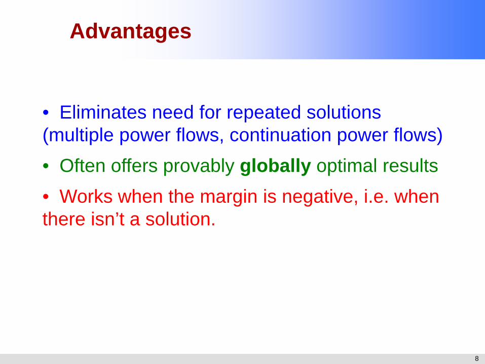
Advantages

• Eliminates need for repeated solutions (multiple power flows, continuation power flows) • Often offers provably globally optimal results • Works when the margin is negative, i.e. when there isn’t a solution.

9


Power

Voltage, V Margin

Optimal Solution

Vopt

V0

P0 Pmax

10

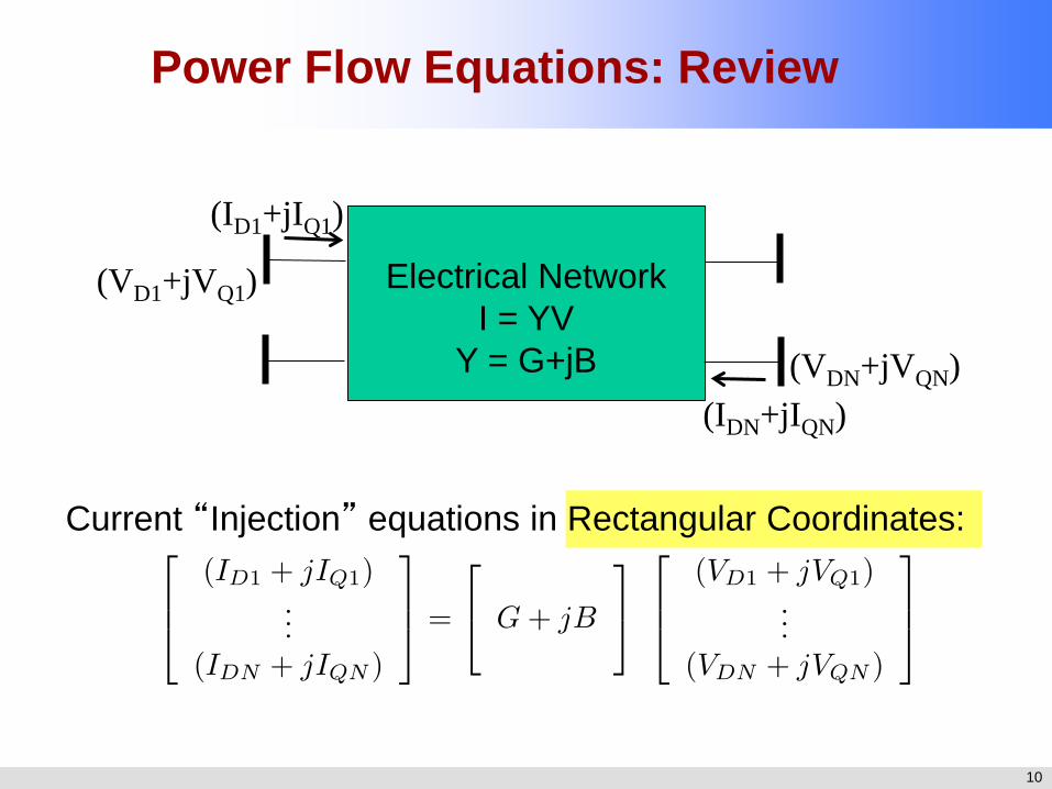
Power Flow Equations: Review

Electrical Network

I = YV Y = G+jB

(ID1+jIQ1)

(IDN+jIQN)

(VD1+jVQ1)

(VDN+jVQN)

Current “Injection” equations in Rectangular Coordinates:

11

Power Flow Equations: Review

Electrical Network

I = YV Y = G+jB

(P1+jQ1)

(PN+jQN)

(VD1+jVQ1)

(VDN+jVQN)

Power “Injection” equations in Rectangular Coordinates:

12

Power Flow Equations

The power flow equations are quadratic in voltage variables:

For reference, power engineers almost always express these equations in voltage polar coordinates:

13

Classical Power Flow Constraints

Bus Type Specified Calculated

PQ (load) P, Q V, δ

PV (generator) P, V Q, δ

Slack V, δ = 0º P, Q

The “controlled voltages” are the problem-specified slack and generator voltage magnitudes. Locking the controlled voltages in constant proportion, and allowing them to scale by α, we claim a power solution exists for any power flow injection profile. (subject to the unimportant small print.)

14

Optimization Problem • Modify the power flow formulation to • Slack bus voltage magnitude unconstrained

• PV bus voltage magnitudes scale with slack bus voltage

• Minimize slack bus voltage

15

This optimization problem can be solved many different ways…

We’ve been using the convex relaxation formulation for the power flow equations (Lavaei, Low) because we really want (provably) the minimum solution.

• The problem has a feasible solution • The optimization using the convex relaxation can be

solved for a global minimum (and hopefully a feasible power flow solution).

Optimization Problem

16

Relaxed Problem Formulation

In Rectangular coordinates, define

Then, power flow equations can be written in the form

where

Which is a rank one matrix by construction.

17

Relaxed Problem Formulation

The convex relaxation is introduced by relaxing the rank of W. With that, we pose the following convex optimization

problem:

18

Semidefinite Relaxation Example

MISDP

19

Semidefinite Relaxation Example

MISDP

20

Bonus result concerning solution to the power flow equations

• The existence of a power flow solution requires

• Necessary, but not sufficient, condition for existence

• Conversely, no solution exists if

• Sufficient, but not necessary, condition for non-existence

21

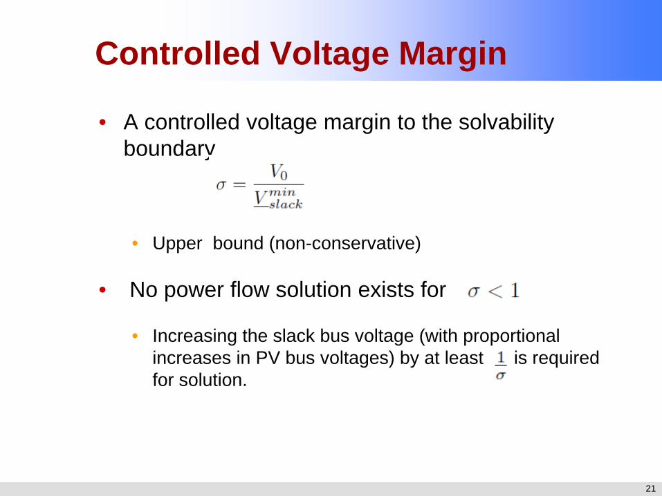
Controlled Voltage Margin

• A controlled voltage margin to the solvability boundary

• Upper bound (non-conservative)

• No power flow solution exists for

• Increasing the slack bus voltage (with proportional increases in PV bus voltages) by at least is required for solution.

22

Power Injection Margin • Uniformly scaling all power injections scales

• Uniformly scale power injections until

• Corresponding gives a power flow voltage stability margin in the direction of uniformly increasing power injections at constant power factor.

• indicates that no solution exists for the original power flow problem

23

Power Injection Margin

The power injection margin answers the question

For a given voltage profile, by what factor can we change our power injections (uniformly at all buses) while still potentially having a solution?

Answer:

24

Examples • IEEE 14-Bus System

• IEEE 118-Bus System

• Tested many other systems and loadings

25

0 0.5 1 1.5 2 2.5 3 3.5 4 4.50.1

0.2

0.3

0.4

0.5

0.6

0.7

0.8

0.9

1

1.1IEEE 14-Bus Continuation Trace: Bus 5

Injection Multiplier

V5


26

0 0.5 1 1.5 2 2.5 3 3.5 4 4.50.1

0.2

0.3

0.4

0.5

0.6

0.7

0.8

0.9

1

1.1IEEE 14-Bus Continuation Trace: Bus 5


V5


27

IEEE 14 Bus System Injection

Multiplier

Newton-Raphson

Converged?

dim(null(A)

1.000 Yes 1.06 0.5261 2 2.000 Yes 1.06 0.7440 2 3.000 Yes 1.06 0.9112 2 4.000 Yes 1.06 1.0522 2 4.010 Yes 1.06 1.0535 2 4.020 Yes 1.06 1.0548 2 4.030 Yes 1.06 1.0561 2 4.040 Yes 1.06 1.0575 2 4.050 Yes 1.06 1.0588 2 4.055 Yes 1.06 1.0594 2 4.056 Yes 1.06 1.0595 2 4.057 Yes 1.06 1.0597 2 4.058 Yes 1.06 1.0598 2 4.059 Yes 1.06 1.0599 2 4.060 No 1.06 1.0601 2 4.061 No 1.06 1.0602 2 4.062 No 1.06 1.0603 2 4.063 No 1.06 1.0605 2 4.064 No 1.06 1.0606 2 4.065 No 1.06 1.0607 2 5.000 No 1.06 1.1764 2

28

Voltage Margin

29

0 0.5 1 1.5 2 2.5 3 3.5 4 4.5 50

0.2

0.4

0.6

0.8

1

1.2

IEEE 14-Bus Continuation Trace: Bus 5


V5

Voltage and Power Injection Margins

30

0 0.5 1 1.5 2 2.5 3 3.50

0.2

0.4

0.6

0.8

1



V44


31

0 0.5 1 1.5 2 2.5 3 3.50

0.2

0.4

0.6

0.8

1



V44


32

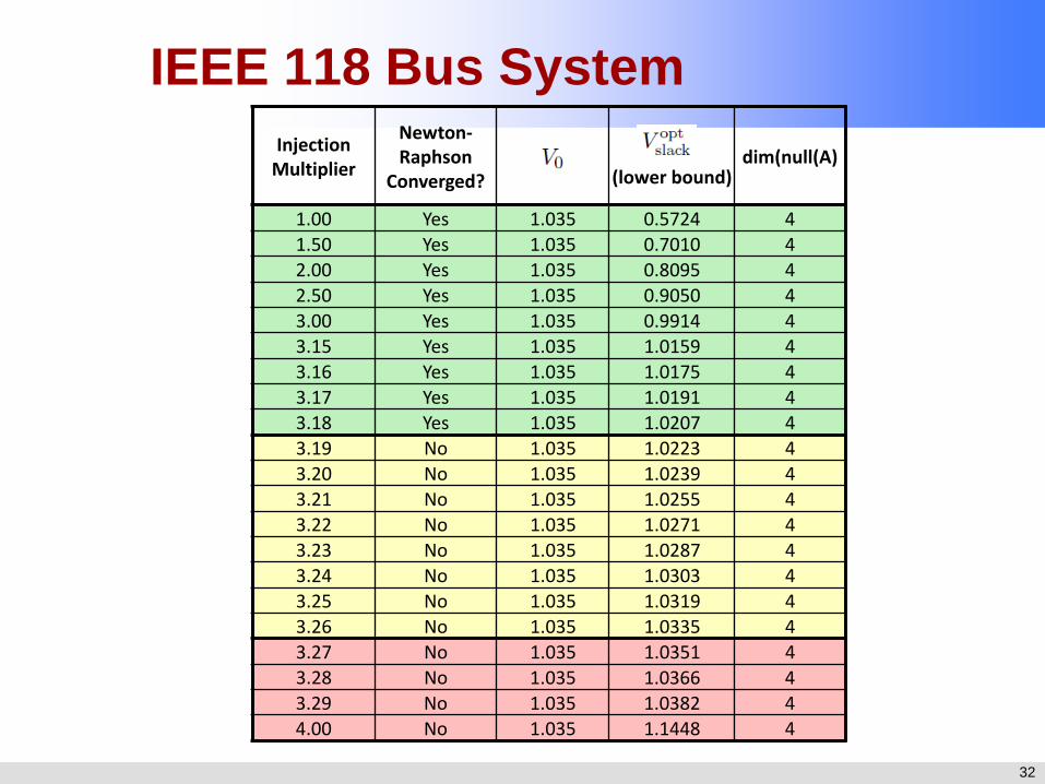
IEEE 118 Bus System Injection

Multiplier

Newton-Raphson

Converged?

(lower bound)

dim(null(A)

1.00 Yes 1.035 0.5724 4 1.50 Yes 1.035 0.7010 4 2.00 Yes 1.035 0.8095 4 2.50 Yes 1.035 0.9050 4 3.00 Yes 1.035 0.9914 4 3.15 Yes 1.035 1.0159 4 3.16 Yes 1.035 1.0175 4 3.17 Yes 1.035 1.0191 4 3.18 Yes 1.035 1.0207 4 3.19 No 1.035 1.0223 4 3.20 No 1.035 1.0239 4 3.21 No 1.035 1.0255 4 3.22 No 1.035 1.0271 4 3.23 No 1.035 1.0287 4 3.24 No 1.035 1.0303 4 3.25 No 1.035 1.0319 4 3.26 No 1.035 1.0335 4 3.27 No 1.035 1.0351 4 3.28 No 1.035 1.0366 4 3.29 No 1.035 1.0382 4 4.00 No 1.035 1.1448 4

33

Voltage Margin IEEE 118 Bus System

34

0 0.5 1 1.5 2 2.5 3 3.5 40

0.2

0.4

0.6

0.8

1

1.2



V44

Voltage and Power Injection Margins

35

Alternate Power Injection Profiles Power injection margin is in the direction of a uniform,

constant-power-factor injection profile

We can alternatively specify any profile that is a linear function of powers and squared voltages

‒ However, insolvability condition is not necessarily valid

36

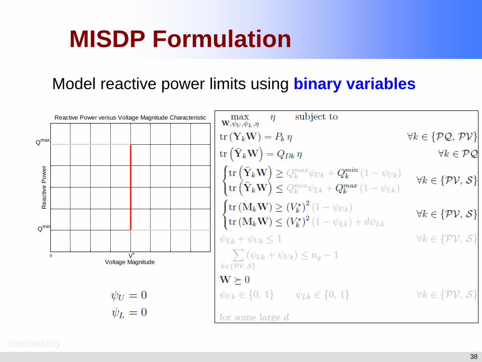
Reactive Power Limits Previous work models generators

as ideal voltage sources

Detailed models limit reactive outputs

‒ Limit-induced bifurcations

Two approaches to modeling these limits:

‒ Mixed-integer semidefinite programming

‒ Infeasibility certificates using sum of squares programming

0

Voltage Magnitude

Rea

ctiv

e P

ower

Reactive Power versus Voltage Magnitude Characteristic

V∗

Qmax

Qmin

37

MISDP Formulation

0

Voltage Magnitude

Rea

ctiv

e P

ower


V∗

Qmin

Qmax

Model reactive power limits using binary variables

Insolvability

38

MISDP Formulation

0

Voltage Magnitude

Rea

ctiv

e P

ower


V∗

Qmin

Qmax


Insolvability

39

MISDP Formulation

0

Voltage Magnitude

Rea

ctiv

e P

ower


V∗

Qmin

Qmax


Insolvability

40

MISDP Formulation

0

Voltage Magnitude

Rea

ctiv

e P

ower


V∗

Qmin

Qmax


Insolvability

41

Reactive Power Limits Results

1 1.1 1.2 1.3 1.40.985

0.99

0.995

1

1.005

1.01

1.015

1.02

1.02514-Bus System Power vs. Voltage

PQ Bus Injection Multiplier

V5

P-V Curve

ηmax

Infeasibility Certificate Found

42

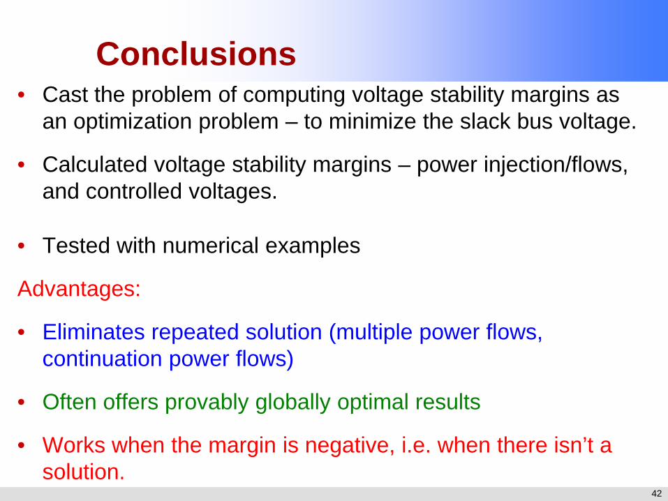
Conclusions • Cast the problem of computing voltage stability margins as

an optimization problem – to minimize the slack bus voltage.

• Calculated voltage stability margins – power injection/flows, and controlled voltages.

• Tested with numerical examples

Advantages:

• Eliminates repeated solution (multiple power flows, continuation power flows)

• Often offers provably globally optimal results

• Works when the margin is negative, i.e. when there isn’t a solution.

43

Related Publications

[1] B.C. Lesieutre, D.K. Molzahn, A.R. Borden, and C.L. DeMarco, “Examining the Limits of the Application of Semidefinite Programming to Power Flow Problems,” 49th Annual Allerton Conference on Communication, Control, and Computing (Allerton), 2011, pp.1492-1499, 28-30 Sept. 2011.

[2] D.K. Molzahn, J.T. Holzer, and B.C. Lesieutre, and C.L. DeMarco, “Implementation of a Large-Scale Optimal Power Flow Solver Based on Semidefinite Programming,” To appear in IEEE Transactions on Power Systems.

[3] D.K. Molzahn, B.C. Lesieutre, and C.L. DeMarco, “An Approximate Method for Modeling ZIP Loads in a Semidefinite Relaxation of the OPF Problem,” submitted to IEEE Transactions on Power Systems, Letters.

[4] D.K. Molzahn, B.C. Lesieutre, and C.L. DeMarco, "A Sufficient Condition for Global Optimality of Solutions to the Optimal Power Flow Problem,” to appear in IEEE Transactions on Power Systems, Letters.

[5] D.K. Molzahn, B.C. Lesieutre, and C.L. DeMarco, “A Sufficient Condition for Power Flow Insolvability with Applications to Voltage Stability Margins,” IEEE Transactions on Power Systems, Vol 28, No. 3, pp. 2592-2601.

[6] D.K. Molzahn, V. Dawar, B.C. Lesieutre, and C.L. DeMarco, “Sufficient Conditions for Power Flow Insolvability Considering Reactive Power Limited Generators with Applications to Voltage Stability Margins,” presented at Bulk Power System Dynamics and Control - IX. Optimization, Security and Control of the Emerging Power Grid, 2013 IREP Symposium, 25-30 Aug. 2013.

[7] D.K. Molzahn, B.C. Lesieutre, and C.L. DeMarco, “Investigation of Non-Zero Duality Gap Solutions to a Semidefinite Relaxation of the Power Flow Equations,” To be presented at the Hawaii International Conference on System Sciences, January 2014.

Conclusion

44

Questions?

45

Extra Slides: Feasibility

46

For lossless systems: 1. Show a solution exists for zero power injections at

PQ buses and zero active power injection at PV buses, for α = 1.

2. Use implicit function theorem to argue that perturbations to zero power injections solutions also exist. Specifically choose one in the direction of desired power injection profile.

3. Exploit the quadratic nature of power flow equations to scale voltages and power to match injection profile.

Feasibility

47

Easy: Construct a solution. • Open Circuit PQ buses for zero power, zero

current injection. • Use Ward-type reduction to eliminate PQ buses.

(not really necessary, but clean) small print

• Choose uniform angle solution for all buses. • Directly use reactive power flow equation to

calculated the reactive power injections at generator buses.

Feasibility: Zero Power Injection Solution

0

0

0

48

Note: Zero Power Injection Solutions for Lossy Systems

• Not all systems have a zero-power injection solution

• Ability to choose θ such that PPV = 0 depends on

• Ratio of VPV to Vslack

• Ratio of g to b

• Systems with small resistances and small voltage magnitude differences are expected to have a zero power injection solution

49

A nearby non-zero solution exists provided the Jacobian is nonsingular. For a connected

lossless system at the zero-power injection solution, the appropriate Jacobian is nonsingular, generically.

small print

Nearby Solutions

50

Exploit the quadratic nature of power flow equations to scale voltages to match desired power profile:

Feasible Solution

51

Extra Slides: Infeasibility Certificates

52

Infeasibility Certificates

Guarantee that a system of polynomial is infeasible

Positivstellensatz Theorem

If such that

then the system of polynomials has no solution

53

Power Flow in Polynomial Form Power Injection and Voltage Magnitude Polynomials

Reactive Power Limit Polynomials

0

Voltage Magnitude

Rea

ctiv

e P

ower


V∗

Qmax

Qmin

54

Power Flow Infeasibility Certificates

Find a sum of squares polynomial of the form

such that

by finding polynomials

Then the power flow equations have no solution.

and sum of squares polynomials

a new method for estimating maximum power … · operating point to the “ nose point ” on a...

Documents