A New Grid Structure for Domain Extension

Bo Zhu∗

Stanford UniversityWenlong Lu∗

Stanford UniversityMatthew Cong∗

Stanford UniversityIndustrial Light + Magic

Byungmoon Kim†

Adobe Systems Inc.Ronald Fedkiw∗

Stanford UniversityIndustrial Light + Magic

Figure 1: Our far-field grid structure provides an extended domain for fluid simulations of smoke, fire, and water. (Left) A fine grid followsthe sphere in order to resolve the fine scale details of the smoke due to object interaction while the extended grid allows the smoke to riseuntil it is off camera – see Figure 5. (Center) A torch that moves through a large extent of the domain uses a fine grid to track the torchmotion while grid extension allows for larger camera angles – see Figure 6. (Right) A large advantage of our extended grid is that it allowsoutgoing waves to avoid reflecting off of grid boundaries thus allowing for a large amount of detail and grid resolution near the region ofinterest without reflected waves.

Abstract

We present an efficient grid structure that extends a uniform gridto create a significantly larger far-field grid by dynamically extend-ing the cells surrounding a fine uniform grid while still maintain-ing fine resolution about the regions of interest. The far-field gridpreserves almost every computational advantage of uniform gridsincluding cache coherency, regular subdivisions for parallelization,simple data layout, the existence of efficient numerical discretiza-tions and algorithms for solving partial differential equations, etc.This allows fluid simulations to cover large domains that are of-ten infeasible to enclose with sufficient resolution using a uniformgrid, while still effectively capturing fine scale details in regions ofinterest using dynamic adaptivity.

CR Categories: I.3.3 [Computer Graphics]: Three-DimensionalGraphics and Realism—Animation

Keywords: fluid simulation, grids, boundary conditions

Links: DL PDF

∗e-mail: {boolzhu,wenlongl,mdcong,fedkiw}@cs.stanford.edu†e-mail: bmkim@adobe.com

1 Introduction

Computer graphics researchers have utilized a number of interest-ing data structures for fluid simulation including run-length encod-ed (RLE) grids [Houston et al. 2006; Irving et al. 2006; Chen-tanez and Muller 2011], octrees [Losasso et al. 2004], particle-based discretizations [Adams et al. 2007; Solenthaler and Pajaro-la 2009; Solenthaler and Gross 2011], velocity-vorticity domaindecompositions [Golas et al. 2012], tetrahedral meshes [Feldmanet al. 2005; Klingner et al. 2006], and Voronoi diagrams [Sin et al.2009; Brochu et al. 2010]. However, uniform grids still remaina mainstay because of a number of advantages: a cache coheren-t memory layout, regular domain subdivisions suitable for paral-lelization, fast iterative solvers such as preconditioned conjugategradient for solving partial differential equations, higher-order in-terpolation schemes which are are often difficult and computation-ally costly to generalize to unstructured data, and the ability to ac-celerate ray tracing algorithms for axis-aligned voxel data. Tech-niques such as adaptive mesh refinement (AMR) [Berger and Oliger1984; Berger and Colella 1989; Sussman et al. 1999] and chimeragrids [Benek et al. 1983; Benek et al. 1985; Dobashi et al. 2008]have remained prevalent because they use a number of Cartesian u-niform grids. Similarly, the FLIP and PIC methods [Zhu and Brid-son 2005; Losasso et al. 2008] use a background uniform grid forprojection.

We focus on a single uniform grid structure as opposed to the multi-ple uniform grid structures used in AMR and chimera grid methodsnoting that for a variety of applications the added computationalcost and complexity of many grids is unwarranted. However, thereare many applications where one would want to use multiple uni-form grids. Considering a single uniform grid, one could still addgenerality by changing the physical layout of the grid to be a mod-ification of computational grid along the lines of curvilinear grids[Anderson et al. 1997]. Typically, a uniform grid exists in compu-tational space and is mapped in some complex way to the physi-cal domain where it can be boundary-fitted, stretched, compressed,etc., and Jacobians of the mapping are stored throughout the grid.

pu uv

v

δx δx δx δx δx δx2δx 2δx2δx 4δx4δx 4δx

δx

δx

δx

δx

δx

δx

2δx

2δx

4δx

2δx

Figure 2: Our far-field grid structure has a uniform Cartesian gridenclosing the viewer’s domain of interest (outlined in blue) and ex-tends much further in each of the other three spatial dimensions toprovide a large simulation domain. There is a one to one mappingfrom the far-field grid structure to the standard uniform Cartesiangrid which allows for exceptional cache coherency, ease of paral-lelism, and a natural mapping to the GPU – just as in the case ofa uniform Cartesian grid. We have made some choices in limitingthe far-field grid structure such as restricting the edge lengths of ex-tended cells to be a power of two times the edges lengths along eachaxis of the uniform Cartesian grid in order to aggressively minimizeoverhead as compared to a standard uniform Cartesian grid.

One drawback of these methods is that given a point in physical s-pace, it is still difficult and computationally expensive (notO(1) ingeneral) to find out which grid cell contains that point.

We propose a simple modification of the uniform grid where onecan simply slide the vertical and horizontal planes left and rightmaintaining a Cartesian grid that allows for simple O(1) lookupsof arbitrary points. Our grid structure can be seen as a subset ofthe general curvilinear/rectilinear grids used in other areas, whilemany optimizations (see Section 2) are made to this special case togain significant computational efficiencies. Related work includesthe far-field grid of Sussman [Sussman and Smereka 1997], whereone layer of grid cells around the outside of the grid was extendedin order to add relaxation to a pressure solver. We found this workhighly motivating and generalize it to extending any number of lay-ers but restrict those extensions in certain ways in order to makethe lookups more efficient. Another related work is the Sorobangrid [Yabe et al. 2004; Takizawa et al. 2007] where planes are s-lid in one dimension, lines in another, and grid points in another.While also motivating, this Soroban grid structure also struggles toidentify the cell in which an arbitrary point is located. In particu-lar, we stress that the cost of identifying the cells in which arbitrarylocations are located as well as all other costs of our far-field gridstructure only incur about a 10% overhead compared to a standarduniform grid.

2 Grid Structure

A far-field grid in three spatial dimensions is constructed by inde-pendently choosing a number of points in each of the three spatialdimensions and then taking the Cartesian product to obtain the lo-cations of the corners of the grid cells. As illustrated in Figure 2,we store our data on this grid in the usual fashion with the scalarpressure at cell centers and velocities at the faces. Computing thecell that contains an arbitrary point in this general representation

Figure 3: Grid structures for the performance test covering domainsizes of .5× 1, 1× 2, 2× 4, and 3× 6. The blue outline shows thefine grid domain of .5× 1.

of the far-field grid requires a binary search along each axis of thegrid and therefore requires O(logNx + logNy + logNz) runtimewhere Nx, Ny , and Nz are the number of points in each dimen-sion. We can improve the asymptotic runtime of this data accessby changing the layout as follows. First, the stretched cells in eachdimension are organized hierarchically into n different layers. Theedge length of a cell in the ith layer where 1 ≤ i ≤ n is given by2i−1δx where δx denotes the edge length of the finest cells on thegrid. For each layer i > 1, we place k−ij stretched cells on the nega-tive side of the previous layer along the jth axis (j ∈ {1, 2, 3}) andk+ij stretched cells on the positive side of the previous layer. Thisparticular implementation allows one to efficiently compute the cellwhich contains an arbitrary point in O(1) time. Recall that on a u-niform grid, locating this cell can be achieved by simply dividingby δx and truncating in each dimension. On the far-field grid, thisis accomplished with the aid of one precomputed one-dimensionalarray for each axis.

If we construct a uniform grid with the finest resolution, then eachcell in the uniform grid will be contained entirely within a cel-l on the far-field grid. For example, the cell in the bottom leftof Figure 3 would contain eight uniform fine grid cells. Thus, ineach spatial dimension we can construct a simple one dimension-al array which contains for each uniform grid cell the far-field cellthat would contain it. In Figure 2, the x-dimension array wouldbe {1, 1, 1, 1, 2, 2, 3, 4, 5, . . .} allowing us to map the uniform cellnumber to the far-field cell number. Once we identify the cell thatcontains an arbitrary point, we can interpolate values from the cor-ners of that cell without any further information. However, MACgrids store information at faces and cell centers requiring a slightlymodified approach. In order to determine the four (eight in threespatial dimensions) nearest neighbors for interpolating velocity orpressure, one needs to know whether a given location lives in thefirst or second half of the grid cell in each of the spatial dimensions.One simple way of encoding this information would be to make ourone dimensional array twice as long and encode the terms in the ar-ray based on whether each half-size fine uniform cell is containedin the first or second half of the far-field cell. For example, using a“−”-sign for the left half and a “+”-sign for the right half of a cel-l one obtains {−1,−1,−1,−1, 1, 1, 1, 1,−2,−2, 2, 2,−3, 3, . . .}for the aforementioned case. These arrays can be precomputed andstored in each dimension separately and therefore incur a negligiblememory cost – and is especially elegant for a GPU implementation.

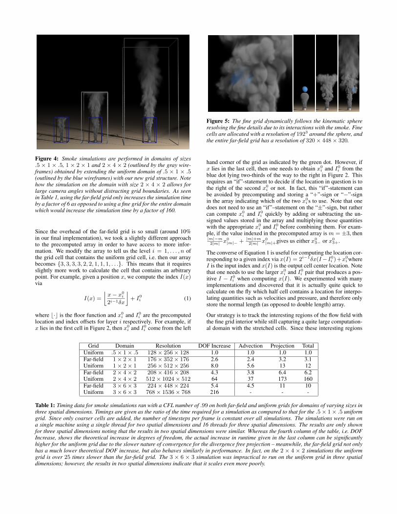
Figure 4: Smoke simulations are performed in domains of sizes.5 × 1 × .5, 1 × 2 × 1 and 2 × 4 × 2 (outlined by the gray wire-frames) obtained by extending the uniform domain of .5 × 1 × .5(outlined by the blue wireframes) with our new grid structure. Notehow the simulation on the domain with size 2 × 4 × 2 allows forlarge camera angles without distracting grid boundaries. As seenin Table 1, using the far-field grid only increases the simulation timeby a factor of 6 as opposed to using a fine grid for the entire domainwhich would increase the simulation time by a factor of 160.

Since the overhead of the far-field grid is so small (around 10%in our final implementation), we took a slightly different approachto the precomputed array in order to have access to more infor-mation. We modify the array to tell us the level i = 1, . . . , n ofthe grid cell that contains the uniform grid cell, i.e. then our arraybecomes {3, 3, 3, 3, 2, 2, 1, 1, 1, . . .}. This means that it requiresslightly more work to calculate the cell that contains an arbitrarypoint. For example, given a position x, we compute the index I(x)via

I(x) =

⌊x− x0i2i−1δx

⌋+ I0i (1)

where b·c is the floor function and x0i and I0i are the precomputedlocation and index offsets for layer i respectively. For example, ifx lies in the first cell in Figure 2, then x0i and I0i come from the left

Figure 5: The fine grid dynamically follows the kinematic sphereresolving the fine details due to its interactions with the smoke. Finecells are allocated with a resolution of 1923 around the sphere, andthe entire far-field grid has a resolution of 320× 448× 320.

hand corner of the grid as indicated by the green dot. However, ifx lies in the last cell, then one needs to obtain x0i and I0i from theblue dot lying two-thirds of the way to the right in Figure 2. Thisrequires an “if”-statement to decide if the location in question is tothe right of the second x0i or not. In fact, this “if”-statement canbe avoided by precomputing and storing a “+”-sign or “−”-signin the array indicating which of the two x0i s to use. Note that onedoes not need to use an “if”–statement on the “±”-sign, but rathercan compute x0i and I0i quickly by adding or subtracting the un-signed values stored in the array and multiplying those quantitieswith the appropriate x0i and I0i before combining them. For exam-ple, if the value indexed in the precomputed array is m = ±3, then|m|−m2|m| x

0|m|− + |m|+m

2|m| x0|m|+gives us either x03− or x03+.

The converse of Equation 1 is useful for computing the location cor-responding to a given index via x(I) = 2i−1δx(I−I0i )+x0i whereI is the input index and x(I) is the output cell center location. Notethat one needs to use the larger x0i and I0i pair that produces a pos-itive I − I0i when computing x(I). We experimented with manyimplementations and discovered that it is actually quite quick tocalculate on the fly which half cell contains a location for interpo-lating quantities such as velocities and pressure, and therefore onlystore the normal length (as opposed to double length) array.

Our strategy is to track the interesting regions of the flow field withthe fine grid interior while still capturing a quite large computation-al domain with the stretched cells. Since these interesting regions

Grid Domain Resolution DOF Increase Advection Projection TotalUniform .5× 1× .5 128× 256× 128 1.0 1.0 1.0 1.0Far-field 1× 2× 1 176× 352× 176 2.6 2.4 3.2 3.1Uniform 1× 2× 1 256× 512× 256 8.0 5.6 13 12Far-field 2× 4× 2 208× 416× 208 4.3 3.8 6.4 6.2Uniform 2× 4× 2 512× 1024× 512 64 37 173 160Far-field 3× 6× 3 224× 448× 224 5.4 4.5 11 10Uniform 3× 6× 3 768× 1536× 768 216 - - -

Table 1: Timing data for smoke simulations ran with a CFL number of .99 on both far-field and uniform grids for domains of varying sizes inthree spatial dimensions. Timings are given as the ratio of the time required for a simulation as compared to that for the .5× 1× .5 uniformgrid. Since only coarser cells are added, the number of timesteps per frame is constant over all simulations. The simulations were run ona single machine using a single thread for two spatial dimensions and 16 threads for three spatial dimensions. The results are only shownfor three spatial dimensions noting that the results in two spatial dimensions were similar. Whereas the fourth column of the table, i.e. DOFIncrease, shows the theoretical increase in degrees of freedom, the actual increase in runtime given in the last column can be significantlyhigher for the uniform grid due to the slower nature of convergence for the divergence free projection – meanwhile, the far-field grid not onlyhas a much lower theoretical DOF increase, but also behaves similarly in performance. In fact, on the 2 × 4 × 2 simulations the uniformgrid is over 25 times slower than the far-field grid. The 3 × 6 × 3 simulation was impractical to run on the uniform grid in three spatialdimensions; however, the results in two spatial dimensions indicate that it scales even more poorly.

Figure 6: A detailed flaming torch is moved and used to illuminate different sections of a large domain (top). The torch is then dropped onthe ground generating trailing flame details as it falls (bottom). The fine grid has a resolution of 1283 and dynamically tracks the level setin order to resolve the visually appealing fine scale flame wrinkles, while the entire far-field grid of resolution 208 × 288 × 208 efficientlyresolves the global motion of the fire and smoke.

are usually around objects or at the point of camera focus, they canpotentially move and change size, which we handle by dynamicallychanging the structure of the far-field grid. This is accomplishedby moving grid lines in each dimension (see Section 4) as motivat-ed by [Yabe et al. 2004; Takizawa et al. 2007]. One can also addand delete grid lines in each dimension noting that one needs tobe careful that the total number of cells does not increase beyondthe original allocation of the array because this would incur the ex-tra cost of reallocating large arrays for three dimensional data. Westress that this does not mean that the grid can never grow in thenumber of cells; it just means that one should preallocate a bufferwhich is large enough to include the maximum number of cells.

3 Incompressible Flow

Our smoke solver follows the general procedure of [Fedkiw et al.2001]. The inviscid incompressible Navier-Stokes equations aregiven by

ut + u · ∇u = −1

ρ∇p+ f , (2)

∇ · u = 0, (3)

where u is the velocity field, ρ is the density, p is the pressure,and f is the sum of any external forces (such as vorticity con-finement, buoyancy, and gravity) scaled by ρ. First we com-pute the intermediate velocity u∗ ignoring the pressure term via(u∗ −un)/∆t+ (un · ∇)un = f making use of semi-Lagrangianadvection [Stam 1999; Kim et al. 2005; Selle et al. 2008] beforecomputing the final velocity as un+1 = u∗ −∆t∇p/ρ. The pres-sure p is calculated by solving a Poisson equation of the form

Vcell∇ ·(∇pρ

)= Vcell∇ · u∗. (4)

where p = p∆t is a scaled pressure, Vcell is the volume of a cel-l, and we have used the volume weighted divergence as outlined in[Losasso et al. 2004] in order to obtain a symmetric positive definitesystem on our stretched grid. Equation 4 can be solved efficientlyusing the preconditioned conjugate gradient method with an incom-plete Cholesky preconditioner.

Invoking the second vector form of Green’s theorem on both sidesof Equation 4, we obtain∑

faces

∇pρ· dAface =

∑faces

u∗face · dAface (5)

where dAface is the area-weighted normal of the face. Note thatalthough the faces are not equidistant between pressure locationswhere the edge length along a particular axis changes, we still com-pute the pressure gradients in the usual way subtracting the adjacentvalues and dividing by the actual distance between the cell center-s. Furthermore, we demonstrate that this pressure discretization onthe far-field grid achieves second-order accuracy as on uniform grid(see Table 2).

We demonstrate the efficacy of our method by simulating smoke onthe grids outlined in Figure 3 where the initial fine grid is paddedfrom left to right with a larger and larger far-field grid demonstrat-ing the significant domain extension obtainable using this approach(see Figure 4 and Table 1).

4 Dynamic Tracking

Solid objects are handled in the usual manner by setting the velocityof cells covered by the object to the object velocity and setting Neu-

Figure 7: A dynamically resizing fine grid with a resolution upto 1603 dynamically tracks the level set in order to resolve localflame details of a torch moving in the wind. The far-field grid has aresolution of 210× 300× 210.

Figure 8: A spherical water drop falls into a large body of water 40 times larger than the spherical drop. The stretched grid cells allow theresulting radially outgoing waves to continue propagating into the coarser domain as opposed to reflecting back into the fine domain. A finegrid with a resolution of 384 × 96 × 384 is placed near the sphere, and the far-field grid has resolution 672 × 120 × 672. This allows thegrid to resolve the initial splash (top) and capture surface details such as the resulting radially outgoing waves that propagate throughout thelarge domain (bottom).

mann boundary conditions inside the object for the pressure solve.The far-field grid can adaptively place the finest discretizations in amoving and resizing region of interest that is a subset of the entirecomputational domain and dynamically track it during the courseof a simulation. Figure 5 shows smoke interacting with a kine-matically driven sphere. At the beginning of each simulation, wechoose a bounding box in the vicinity of the object and precomputea translation from the center of the bounding box to the center ofthe object maintaining that offset throughout the simulation. Thefine region of the far-field grid lies entirely within this boundingbox, and the grid lines are redistributed such that the resulting newstretched cells encompass the rest of the domain. This allows us toresolve fine scale fluid details in the vicinity of the object.

Solving the Navier-Stokes equations on a grid that dynamicallytracks an object requires storing the grid structure both at time tn

and tn+1 so that the velocity field can be interpolated from the timetn grid to the time tn+1 grid in order to trace the semi-Lagrangianrays backward in time and interpolate from the time tn grid. Theprojection step does not require modification.

We demonstrate the use of the far-field grid for fire simulation inFigures 6 and 7 using the thin flame model [Nguyen et al. 2002](see also [Hong et al. 2007]). A dynamic surface where the chem-ical reaction occurs is represented with a level set, and Rankine-Hugoniot jump conditions for velocity and pressure are enforcedacross the interface in order to conserve mass and momentum. Re-acted and unreacted materials are distinguished with densities of ρr

Grid L1 Error Order L∞ Error Order128× 128 1.68× 10−4 – 1.02× 10−3 –256× 256 4.17× 10−5 2.01 2.54× 10−4 2.01512× 512 1.04× 10−5 2.01 6.33× 10−5 2.01

1024× 1024 2.59× 10−6 2.00 1.58× 10−5 2.002048× 2048 6.58× 10−7 1.98 3.93× 10−6 2.01

Table 2: Poisson solver accuracy on the far-field grid. A Poissonequation with an analytic solution of φ(x, y) = sin(πx) sin(πy) issolved on a far-field grid.

and ρu respectively in Equation 2. The Poisson equation with pres-sure jumps across the interface is solved on the far-field grid usingthe volume weighted divergence discussed in Section 3. In eachtimestep the level set interface is evolved by advecting the signeddistance function φ and applying the fast marching method. All ofthese discretizations are straightforward to apply since the far-fieldgrid is also a Cartesian grid.

However, in order resolve the detailed flame wrinkles around thelevel set interface, it is preferable to enclose the level set which canmove independently of the torch (e.g. due to wind). We accomplishthis in two steps. First, we track the torch by translating the entirefar-field grid by adding or removing cells as in [Rasmussen et al.2004] (see also [Shah et al. 2004; Cohen et al. 2010]). Second, thefine grid dynamically moves around in the interior of the far-fieldgrid in order to track the level set representation of the flame. Thisis accomplished by computing the level set’s bounding box at eachtime step and clamping it to a maximum and minimum size alongeach dimension.

5 Non-Reflecting Waves

Our fluid solver for free surface flows uses the particle level setmethod of [Enright et al. 2002]. A constant number of positiveand negative particles are seeded per cell within a distance of 3δx(stressing that this is the fine grid δx) from the interface. Since wewould like to resolve fine scale details on the fine grid, we prefer alarge number of particles on the fine grid. In contrast, we place acoarse grid where we expect to lose detail due to numerical dissipa-tion and therefore require fewer particles in the coarse regions. Inthe projection step, we use the pressure modifications of [Enrightet al. 2003] to achieve second order accuracy at the free surface.The fast marching method is used to maintain the signed distanceproperty of φ in the vicinity of the interface and velocity extrapo-lation is performed using closest point extrapolation to ensure thatthe interface moves unhindered by the air. Again, we stress thatthe Cartesian nature of our underlying grid makes all of these dis-cretizations straightforward to apply. We demonstrate our solver forfree surface flows in Figures 8, 9, and 10. (Figure 10 uses vortexparticles [Selle et al. 2005].)

Figure 10: A fine grid dynamically follows a boat allowing the simulation to capture fine scale details of the wake in the presence of far-fieldboundary conditions. Vortex particles are seeded behind the boat in order to generate additional fine scale details. The fine grid has aresolution of 192× 32× 192 and the far-field grid has a resolution of 384× 58× 320.

It is often computationally intractable to sufficiently approximatefar-field boundary conditions on a uniform grid while preserving ahigh-degree of detail. The domain needs to be large enough to en-close the fluid flow without boundaries influencing the fluid motionwhile a sufficient number of cells still need to be placed through-out the domain in order to resolve the fine scale details in the re-gions of interest. Thus, researchers have explored various methodsfor approximating far-field boundary conditions such as perfectlymatched layers [Soderstrom et al. 2010]. Our grid structure is ableto efficiently approximate far-field boundary conditions by progres-sively extending the grid cells as one moves farther away from thefine uniform grid covering the region of interest. Since numericalviscosity often damps out fine scale features in the fluid flow be-fore reaching the boundary, the extended grid cells can sufficientlyresolve the flow far away from the highest resolution domain sur-rounding the region of interest at a much lower computational costcompared to placing uniform cells throughout the domain. Further-more, we have verified that the outgoing wave propagation speedfor the simulation shown in Figure 8 is the same on both the far-field grid and the corresponding uniform grid (where the cell sizeon the uniform grid is the same as that in the fine region of thefar-field grid).

We have noticed that if the fine grid is insufficiently large com-pared to the initial splash and transitions to the coarser grid beforethe outgoing waves are sufficiently dissipated, the lower frequencycomponents of the waves are transmitted into the coarser domainwhile the higher frequency components of the waves can be reflect-ed back into the fine domain. This results in artificial interferencepatterns which are especially noticeable in the case of the fallingspherical water drop due to the radial nature of the outgoing waves.An alternative solution (that we do not follow) for alleviating thesereflected waves is to dynamically resize the fine grid such that theradially outward propagating initial wave generated by the splash isalways enclosed in the fine region. This approach causes the speed

Figure 9: A solid armadillo falls into a large body of water whichenforces a far-field boundary condition. The fine grid has a reso-lution of 384 × 96 × 384 and the far-field grid has a resolution of672× 168× 672.

of the simulation to decrease significantly as the simulation pro-gresses since the fine grid needs to be expanded along two of thethree dimensions. On the other hand, these extra grid lines can beremoved after the splash dissipates.

6 Extensions and Conclusions

We have presented an efficient grid structure that extends a uniformgrid to create a significantly larger far-field grid that is a heavily-optimized special case of existing curvilinear grids. Our approachpreserves almost every computational advantage of uniform gridsincluding cache coherency, regular subdivisions for parallelization,simple data layout, and the existence of efficient numerical algo-rithms for solving partial differential equations due to the under-lying Cartesian nature of our grid. We demonstrate that our gridstructure allows us to simulate significantly larger domains than auniform grid thus allowing us to capture far-field boundary condi-tions while maintaining the same resolution in regions of interest.Efficient algorithms for ray tracing axis-aligned voxel data on uni-form grids are straightforward to adapt to the far-field grid whichwe demonstrate by performing all of our lighting precomputationand rendering directly on the far-field grid.

While our specific implementation is unable to simultaneouslytrack multiple regions of interest with fine grids on a single far-field grid, one could instead track multiple regions by overlayingmultiple far-field grids that each have a single region of interest.This adds additional fine regions at the cost of maintaining multiplehierarchical subdivisions. In fact, an AMR or chimera grid imple-mentation could readily make use of one or more far-field grids.Another approach is to relax our restrictions on the general far-fieldgrid and allow for multiple fine regions on a single far-field gridby choosing multiple regions of fine grid points along each axis.However, this approach leads to additional fine regions in areas thatare not regions of interest since the fine regions in the far-field gridare determined by the Cartesian product of the fine regions alongeach axis. For example, if we wanted to track two objects with fineuniform grids located at (x1, y1) and (x2, y2) in two spatial dimen-sions, we would also be forced to resolve the regions surrounding(x1, y2) and (x2, y1) resulting in four fine regions.

There are also visual artifacts that can arise due to the stretched cell-s. In smoke simulations, there is an increased amount of numericaldissipation in regions with stretched cells which can manifest whenthe smoke density field is rendered. In fire simulations, a similarproblem exists with the temperature field but can be resolved byenclosing the region of interest (level set wrinkles) within the finestdiscretization since a fire simulation is often localized. In watersimulations, the increased dissipation in stretched regions tends torapidly smooth out the sharp features of the free surface. How-ever, outside of the region of interest, there are usually fewer of

these sharp features and the increased numerical dissipation is lessnoticeable. Thus, the far-field grid is more suitable to modelinglocalized fluid phenomena with a bounded region of interest suchas fire and water as opposed to smoke where the density tends todistribute itself throughout the entire domain.

Another interesting direction for future work is the implementationof the far-field grid on the GPU towards real time applications. Thefar-field grid can be represented in three spatial dimensions usingthree small one-dimensional arrays or textures which can be boundeither as constants or small texture or stored in group shared mem-ory. Due to the Cartesian nature of the far-field grid, the data storedon the far-field grid has a direct mapping to three-dimensional tex-tures or arrays and therefore numerical algorithms optimized for u-niform grids on the GPU can be easily adapted to operate on the far-field grid. The far-field grid’s ability to dynamically resolve detailsinside a region of interest within a very large domain while main-taining almost every computational advantage of a uniform grid hasthe potential to facilitate the use of fluid simulations in numerousreal time applications.

Acknowledgements

Research was supported in part by ONR N00014-09-1-0101, ON-R N-00014-11-1-0027, ONR N00014-11-1-0707, ARL AHPCRCW911NF-07-0027, and the Intel Science and Technology Centerfor Visual Computing. Computing resources were provided in partby ONR N00014-05-1-0479. We would like to thank Jure Leskovecand Christos Kozyrakis for additional computing resources as wellas Andrej Krevl and Jacob Leverich for helping us use those re-sources.

References

ADAMS, B., PAULY, M., KEISER, R., AND GUIBAS, L. J. 2007.Adaptively sampled particle fluids. ACM Trans. Graph. (SIG-GRAPH Proc.) 26, 3.

ANDERSON, D. A., TANNEHILL, J. C., AND PLETCHER, R. H.1997. Computational Fluid Mchanics and Heat Transfer. Taylor& Francis, 531.

BENEK, J. A., STEGER, J. L., AND DOUGHERTY, F. C. 1983. Aflexible grid embedding technique with applications to the eulerequations. In 6th Computational Fluid Dynamics Conference,AIAA, 373–382.

BENEK, J. A., BUNING, P. G., AND STEGER, J. L. 1985. A 3-dchimera grid embedding technique. In 7th Computational FluidDynamics Conference, AIAA, 322–331.

BERGER, M., AND COLELLA, P. 1989. Local adaptive mesh re-finement for shock hydrodynamics. J. Comput. Phys. 82, 64–84.

BERGER, M., AND OLIGER, J. 1984. Adaptive mesh refinementfor hyperbolic partial differential equations. J. Comput. Phys.53, 484–512.

BROCHU, T., BATTY, C., AND BRIDSON, R. 2010. Matching fluidsimulation elements to surface geometry and topology. ACMTrans. Graph. (SIGGRAPH Proc.), 47:1–47:9.

CHENTANEZ, N., AND MULLER, M. 2011. Real-time eulerianwater simulation using a restricted tall cell grid. ACM Trans.Graph. (SIGGRAPH Proc.) 30, 4, 82:1–82:10.

COHEN, J. M., TARIQ, S., AND GREEN, S. 2010. Interactivefluid-particle simulation using translating eulerian grids. In Proc.

of the 2010 ACM SIGGRAPH Symp. on Interactive 3D Graphicsand Games, 15–22.

DOBASHI, Y., MATSUDA, Y., YAMAMOTO, T., AND NISHITA,T. 2008. A fast simulation method using overlapping grids forinteractions between smoke and rigid objects. Comput. Graph.Forum 27, 2, 477–486.

ENRIGHT, D., MARSCHNER, S., AND FEDKIW, R. 2002. Ani-mation and rendering of complex water surfaces. ACM Trans.Graph. (SIGGRAPH Proc.) 21, 3, 736–744.

ENRIGHT, D., NGUYEN, D., GIBOU, F., AND FEDKIW, R. 2003.Using the particle level set method and a second order accu-rate pressure boundary condition for free surface flows. In Proc.4th ASME-JSME Joint Fluids Eng. Conf., number FEDSM2003–45144. ASME.

FEDKIW, R., STAM, J., AND JENSEN, H. 2001. Visual simulationof smoke. In Proc. of ACM SIGGRAPH 2001, 15–22.

FELDMAN, B., O’BRIEN, J., KLINGNER, B., AND GOKTEKIN,T. 2005. Fluids in deforming meshes. In Proc. of the ACMSIGGRAPH/Eurographics Symp. on Comput. Anim., 255–259.

GOLAS, A., NARAIN, R., SEWALL, J., KRAJCEVSKI, P., DUBEY,P., AND LIN, M. 2012. Large-scale fluid simulation usingvelocity-vorticity domain decomposition. ACM Trans. Graph.31, 6, 148:1–148:9.

HONG, J., SHINAR, T., AND FEDKIW, R. 2007. Wrinkled flamesand cellular patterns. ACM Trans. Graph. (SIGGRAPH Proc.)26, 3, 47.

HOUSTON, B., NIELSEN, M., BATTY, C., NILSSON, O., ANDMUSETH, K. 2006. Hierarchical RLE level set: A compact andversatile deformable surface representation. ACM Trans. Graph.25, 1, 1–24.

IRVING, G., GUENDELMAN, E., LOSASSO, F., AND FEDKIW, R.2006. Efficient simulation of large bodies of water by couplingtwo and three dimensional techniques. ACM Trans. Graph. (SIG-GRAPH Proc.) 25, 3, 805–811.

KIM, B.-M., LIU, Y., LLAMAS, I., AND ROSSIGNAC, J. 2005.Flowfixer: Using BFECC for fluid simulation. In EurographicsWorkshop on Natural Phenomena 2005.

KLINGNER, B. M., FELDMAN, B. E., CHENTANEZ, N., ANDO’BRIEN, J. F. 2006. Fluid animation with dynamic meshes.ACM Trans. Graph. (SIGGRAPH Proc.) 25, 3, 820–825.

LOSASSO, F., GIBOU, F., AND FEDKIW, R. 2004. Simulating wa-ter and smoke with an octree data structure. ACM Trans. Graph.(SIGGRAPH Proc.) 23, 457–462.

LOSASSO, F., TALTON, J., KWATRA, N., AND FEDKIW, R. 2008.Two-way coupled sph and particle level set fluid simulation.IEEE TVCG 14, 4, 797–804.

NGUYEN, D., FEDKIW, R., AND JENSEN, H. 2002. Physical-ly based modeling and animation of fire. ACM Trans. Graph.(SIGGRAPH Proc.) 21, 721–728.

RASMUSSEN, N., ENRIGHT, D., NGUYEN, D., MARINO, S.,SUMNER, N., GEIGER, W., HOON, S., AND FEDKIW, R. 2004.Directable photorealistic liquids. In Proc. of the 2004 ACM SIG-GRAPH/Eurographics Symp. on Comput. Anim., 193–202.

SELLE, A., RASMUSSEN, N., AND FEDKIW, R. 2005. A vortexparticle method for smoke, water and explosions. ACM Trans.Graph. (SIGGRAPH Proc.) 24, 3, 910–914.

SELLE, A., FEDKIW, R., KIM, B., LIU, Y., AND ROSSIGNAC, J.2008. An Unconditionally Stable MacCormack Method. J. Sci.Comp. 35, 2, 350–371.

SHAH, M., COHEN, J. M., PATEL, S., LEE, P., AND PIGHIN, F.2004. Extended galilean invariance for adaptive fluid simulation.In Proc. of the 2004 ACM SIGGRAPH/Eurographics Symp. onComput. Anim., 213–221.

SIN, F., BARGTEIL, A. W., AND HODGINS, J. K. 2009. A point-based method for animating incompressible flow. In Proceedingsof the 2009 ACM SIGGRAPH/Eurographics Symp. on Comput.Anim., ACM, New York, NY, USA, SCA ’09, 247–255.

SODERSTROM, A., KARLSSON, M., AND MUSETH, K. 2010. Apml-based nonreflective boundary for free surface fluid anima-tion. ACM Trans. Graph. 29, 5, 136:1–136:17.

SOLENTHALER, B., AND GROSS, M. 2011. Two-scale particlesimulation. ACM Trans. Graph. (SIGGRAPH Proc.) 30, 4, 81:1–81:8.

SOLENTHALER, B., AND PAJAROLA, R. 2009. Predictive-corrective incompressible sph. ACM Trans. Graph. (SIGGRAPHProc.) 28, 3, 40:1–40:6.

STAM, J. 1999. Stable fluids. In Proc. of SIGGRAPH 99, 121–128.

SUSSMAN, M., AND SMEREKA, P. 1997. Axisymmetric freeboundary problems. J. Fluid Mech. 341, 269–294.

SUSSMAN, M., ALGREM, A. S., BELL, J. B., COLELLA, P.,HOWELL, L. H., AND WELCOME, M. L. 1999. An adaptivelevel set approach for incompressible two-phase flow. J. Comput.Phys 148, 81–124.

TAKIZAWA, K., YABE, T., TSUGAWA, Y., TEZDUYAR, T. E.,AND MIZOE, H. 2007. Computation of free-surface flows andfluid object interactions with the cip method based on adaptivemeshless soroban grids. Comput. Mech. 40, 1, 167–183.

YABE, T., MIZOE, H., TAKIZAWA, K., MORIKI, H., IM, H.-N.,AND OGATA, Y. 2004. Higher-order schemes with cip methodand adaptive soroban grid towards mesh-free scheme. J. Comput.Phys. 194, 1.

ZHU, Y., AND BRIDSON, R. 2005. Animating sand as a fluid.ACM Trans. Graph. (SIGGRAPH Proc.) 24, 3, 965–972.