a new estimation of the recent tropospheric molecular ... · 3376 c. e. yver et al.: h2 data...

Atmos. Chem. Phys., 11, 3375–3392, 2011www.atmos-chem-phys.net/11/3375/2011/doi:10.5194/acp-11-3375-2011© Author(s) 2011. CC Attribution 3.0 License.

AtmosphericChemistry

and Physics

A new estimation of the recent tropospheric molecular hydrogenbudget using atmospheric observations and variational inversion

C. E. Yver1, I. C. Pison1,2, A. Fortems-Cheiney1, M. Schmidt1, F. Chevallier1, M. Ramonet1, A. Jordan3, O. A. Søvde4,A. Engel5, R. E. Fisher6, D. Lowry6, E. G. Nisbet6, I. Levin7, S. Hammer7, J. Necki8, J. Bartyzel8, S. Reimann9,M. K. Vollmer 9, M. Steinbacher9, T. Aalto10, M. Maione11, J. Arduini 11, S. O’Doherty12, A. Grant12, W. T. Sturges13,G. L. Forster13, C. R. Lunder14, V. Privalov15, N. Paramonova15, A. Werner16, and P. Bousquet1,2

1Laboratoire des Sciences du Climat et de l’Environnement (LSCE), Gif-sur-Yvette, France2Universite de Versailles Saint-Quentin-en-Yvelines (UVSQ), Versailles, France3Max-Planck Institut fur Biogeochemie, Jena, Germany4University of Oslo, Oslo, Norway5Institut fur Meteorologie und Geophysik, Goethe-Universitat Frankfurt, Frankfurt, Germany6Department of Earth Sciences, Royal Holloway, University of London, Egham, UK7Institut fur Umweltphysik, Heidelberg Universitat, Heidelberg, Germany8Faculty of Physics and Applied Computer Science, AGH-University of Science and Technology, Krakow, Poland9Empa, Swiss Federal Institute for Materials Science and Technology, Laboratory for Air Pollution/EnvironmentalTechnology, Duebendorf, Switzerland10Finnish Meteorological Institute, Climate Change Research, Helsinki, Finland11Universita degli Studi di Urbino, DiSBeF, Sezione di Scienze Chimiche, Urbino, Italy12School of Chemistry, University of Bristol, UK13School of Environmental Sciences, University of East Anglia, Norwich, UK14Norsk Institutt for Luftforskning, Kjeller, Norway15Voeikov Main Geophysical Observatory, St. Petersburg, Russia16Deutscher Wetterdienst, Meteorologisches Observatorium, Hohenpeissenberg, Germany

Received: 18 October 2010 – Published in Atmos. Chem. Phys. Discuss.: 25 November 2010Revised: 25 February 2011 – Accepted: 2 April 2011 – Published: 11 April 2011

Abstract. This paper presents an analysis of the recent tro-pospheric molecular hydrogen (H2) budget with a particularfocus on soil uptake and European surface emissions. A vari-ational inversion scheme is combined with observations fromthe RAMCES and EUROHYDROS atmospheric networks,which include continuous measurements performed betweenmid-2006 and mid-2009. Net H2 surface flux, then depo-sition velocity and surface emissions and finally, depositionvelocity, biomass burning, anthropogenic and N2 fixation-related emissions were simultaneously inverted in severalscenarios. These scenarios have focused on the sensibilityof the soil uptake value to different spatio-temporal distribu-tions. The range of variations of these diverse inversion sets

Correspondence to:C. E. Yver([email protected])

generate an estimate of the uncertainty for each term of theH2 budget. The net H2 flux per region (High Northern Hemi-sphere, Tropics and High Southern Hemisphere) varies be-tween−8 and+8 Tg yr−1. The best inversion in terms of fitto the observations combines updated prior surface emissionsand a soil deposition velocity map that is based on bottom-up and top-down estimations. Our estimate of global H2 soiluptake is−59±9 Tg yr−1. Forty per cent of this uptake is lo-cated in the High Northern Hemisphere and 55% is locatedin the Tropics. In terms of surface emissions, seasonality ismainly driven by biomass burning emissions. The inferredEuropean anthropogenic emissions are consistent with inde-pendent H2 emissions estimated using a H2/CO mass ratio of0.034 and CO emissions within the range of their respectiveuncertainties. Additional constraints, such as isotopic mea-surements would be needed to infer a more robust partitionof H2 sources and sinks.

Published by Copernicus Publications on behalf of the European Geosciences Union.

http://creativecommons.org/licenses/by/3.0/

3376 C. E. Yver et al.: H2 data assimilation

1 Introduction

With a mixing ratio of about 530 ppb (parts per billion,10−9), H2 is the second most abundant reduced trace gasin the troposphere after methane (CH4). In contrast to CH4and other trace gases sharing anthropogenic sources, the ob-served H2 mixing ratios are lower in the Northern Hemi-sphere when compared to the Southern Hemisphere due tothe distribution of the sources and sinks of H2 (Novelli et al.,1999). The strength of each term of the H2 budget is givenhereafter as referred to in the literature (Novelli et al., 1999;Hauglustaine and Ehhalt, 2002; Sanderson et al., 2003; Rheeet al., 2006; Xiao et al., 2007; Price et al., 2007; Ehhalt andRohrer, 2009) and compiled inEhhalt and Rohrer(2009).The main sources of H2 are photochemical production bythe transformation of formaldehyde (HCHO) in the atmo-sphere and incomplete combustion processes. Photolysis ofHCHO, a product in the oxidation chain of methane andother volatile organic compounds (VOCs) accounts for 31 to77 Tg yr−1 and represents half of the total H2 source. Fossilfuel and biomass burning emissions, two incomplete com-bustion sources, account for similar shares of the global H2budget (5−25 Tg yr−1). H2 emissions (3−22 Tg yr−1) orig-inating from nitrogen fixation in the continental and marinebiosphere complete the sources. H2 oxidation by free hy-droxyl radicals (OH) and enzymatic H2 destruction in soilsmust balance these sources because tropospheric H2 does notshow a significant long term trend (Grant et al., 2010). H2 ox-idation through OH accounts for 14 to 24 Tg yr−1, which isequivalent to 15% to 25% of the total H2 sink. H2 soil uptake,the major sink in the budget (40 to 90 Tg yr−1 or 75% to 85%of the total sink), is responsible for the observed latitudinalgradient. It is, however, relatively poorly constrained due touncertainties regarding its associated physical and chemicalprocesses. Specifically, H2 uptake is driven by enzymaticand microbial activities linked to H2 diffusivity, which de-pend mostly on soil moisture and temperature. The variationsof these parameters lead to a seasonal cycle. In the North-ern Hemisphere, the maximum uptake is observed at the endof summer/beginning of autumn when the temperatures aremild and the moisture is weak, leading to high bacterial ac-tivity and good diffusion of air in the soil. The minimumappears to be in spring when the soils are moist and cold,leading to a smaller bacterial activity and a slower diffusionof air in the soils (Conrad and Seiler, 1981, 1985; Yonemuraet al., 1999, 2000a,b; Lallo et al., 2008, 2009; Schmitt et al.,2009).

Although global studies of H2 mixing ratios using obser-vations from sampling networks began in the 1990s,Schmidt(1978) had already presented meridional profiles of the At-lantic Ocean from ship cruise measurements. Subsequently,Khalil and Rasmussen(1990) announced an increase in H2mean mixing ratio based on weekly samplings between 1985and 1989 at six locations from 71.5◦ N to 71.4◦ S. Novelliet al. (1999) presented the first estimation of the H2 budget

using observations from the NOAA Earth System ResearchLaboratory network (52 stations), which covers mainly theNorthern Hemisphere but also to some extent the SouthernHemisphere with oceanic samplings and Antarctic sites. Thisnetwork has been managed for H2 since 1989 with regards tothe first sites and has been progressively extended to includeall of the 52 sites in 1994. The CSIRO Global Flask Sam-pling Network (ten stations) began sampling in 1992 with afocus on the Southern Hemisphere (Langenfelds et al., 2002).Finally, within the AGAGE program (Advanced Global At-mospheric Gases Experiment), H2 has been measured con-tinuously since 1993 at two stations (Prinn et al., 2000). Asmall increasing trend was extracted from the analysis of theobservations provided by the NOAA network (Novelli et al.,1999) whereas the CSIRO observations exhibited a small de-crease (Langenfelds et al., 2002). Since 2006, in the frameof the European project EUROHYDROS, a H2 monitoringnetwork, focusing mainly on Europe (13 continuous and 11flask sampling sites) but also worldwide through 7 flask sam-pling sites outside Europe, was developed (Engel, 2009). TheFrench Atmospheric Network for Greenhouse Gases Moni-toring (RAMCES), part of the Laboratory for Climate andEnvironmental Sciences (LSCE) has provided observationsfrom 11 sites (one of them sampling continuously) to the EU-ROHYDROS network and contributed with 8 additional sitesto this study.

Parallel to the observations, forward modelling studieswere used to provide the first constraints on the H2 budget(Hauglustaine and Ehhalt, 2002; Price et al., 2007). Never-theless, since the soil sink, the major loss term, is only knownwith large uncertainties, it is represented in models with moreor less simplified assumptions which lead to a wide rangeof estimations for every term of the budget and especiallyfor the soil sink, ranging from 40 to 90 Tg yr−1 (Ehhalt andRohrer, 2009).

Atmospheric observations combined with a chemistry-transport model and prior information on surface fluxes andsources and sinks within the atmosphere allow us to retrievethe estimations of the H2 sources and sinks and their un-certainties within a Bayesian inversion framework. Atmo-spheric inversions have already been developed to study H2,but the studies remain sparse:Xiao et al.(2007) have used a2D latitude-vertical 12 box model for atmospheric chemistryin an inversion framework combined with AGAGE, NOAAand CSIRO measurements to estimate the magnitude andvariability of H2 sources and sinks for four semi-hemispheresover the 1993–2004 period.Pison et al.(2009) presenteda first inversion of H2 using the same simplified chemistryscheme and model as in this study. More recently,Bous-quet et al.(2011) have provided an analysis of global-to-sub-continental details in the H2 budget before 2005 basedon an optimisation system at sub-continental scale and usingdiscrete observations from the flask networks of NOAA andCSIRO.

Atmos. Chem. Phys., 11, 3375–3392, 2011 www.atmos-chem-phys.net/11/3375/2011/

C. E. Yver et al.: H2 data assimilation 3377

Table 1. Flask sampling network sites (∗ RAMCES network (LSCE) sites additional to EUROHYDROS network). LSCE: Laboratoire desSciences du Climat et de l’Environnement, France; MPI-BGC: Max Planck Institut fur Biogeochemie, Germany; RHUL: Royal Holloway,University of London, UK; UHEI-IUP: Universitat Heidelberg, Institut fur Umweltphysik, Germany.

Code Site Latitude (◦) Longitude (◦) Altitude (m) Beginning of Isotopes LaboratoriesH2 analysis

(mm/yy)

ALT Alert 82.45 −62.52 210 05/07 no LSCEALT Alert 82.45 −62.52 210 10/04 no MPI-BGCALT Alert 82.45 −62.52 210 10/04 no UHEI-IUPAMS Amsterdam Island −37.95 77.53 150 01/05 yes LSCEBGU Begur 41.97 03.3 30 09/05 no LSCEBIA Bialystok 53.14 23.01 182 01/05 no MPI−BGCCGO* Cape Grim −40.68 144.68 94 03/06 no LSCECPT Cape Point −34.35 18.48 260 03/05 no LSCECVR Cabo Verde 16.52 −24.52 18 03/07 yes MPI-BGCFIK Finokalia 35.34 25.67 152 07/06 no LSCEGRI* Griffin 56.62 −03.78 800–2000 02/06 no LSCEHLE Hanle 32.78 78.96 4301 05/05 no LSCEHNG* Hegyhatsal 46.95 16.65 344 07/05 no LSCEIVI* Ivittuut 61.20 −48.18 15 09/07 no LSCELPO Ile Grande 48.80 −03.57 30 02/06 no LSCEMHD Mace Head 53.33 −9.90 25 01/06 yes LSCENMY Neumayer −70.65 −8.25 42 02/04 yes UHEIOXK Ochsenkopf 53.14 23.01 1022 05/05 no MPI-BGCORL* Orleans 47.8 02.5 100−3000 06/05 no LSCEPDM Pic du Midi 42.93 0.13 2877 09/05 no LSCEPON* Pondichery 12.01 79.86 30 09/06 no LSCEPUY Puy de Dome 45.77 02.97 1465 03/06 no LSCESCH Schauinsland 47.92 7.92 1205 03/05 yes UHEI-IUPSIS Shetland Island 60.05 −1.15 30 10/03 no MPI-BGCTRO Troodos 35.07 −32.88 362 03/07 no RHULTR3* Trainou 47.96 02.11 311 08/06 no LSCETVR* Tver 82.45 −62.52 500–3000 08/04 no LSCEZOT Zotino 60.48 89.21 114 06/01 no MPI−BGC

In this paper, we present the mixing ratio measurementsof the RAMCES and EUROHYDROS sampling networks(13 continuous stations and 26 flasks sampling sites) for H2between July 2006 and July 2009. These time series pro-vide information on seasonal cycles and H2 distribution withlatitude. As no NOAA data were available for this period,we have chosen to use only the data from the RAMCES andEUROHYDROS networks. The observations from mid-2006to mid-2009 are assimilated in a variational inversion to es-timate the global H2 budget. Contrary toBousquet et al.(2011), the observations are continuous as well as discrete,from a more recent period and they are centred on Europe.Bousquet et al.(2011) showed that the 2000s flask networkfor H2 alone could constrain neither the different componentsof the H2 cycle, nor the regional fluxes. Nevertheless, weseparately invert the different sources and sinks, at modelresolution, in order to limit the aggregation error (Kamin-ski et al., 2000); if grouped before inversion, an error in thespatio-temporal distribution of H2 flux cannot be corrected

properly by the inversion. Performing an analysis of the fulluncertainties associated to every term of the budget laid how-ever beyond the scope of this study. Therefore, we presentthe results for large latitudinal bands with a focus on soil up-take. As the density of measurements in time and space ismuch higher in Europe than inBousquet et al.(2011) for thelate 2000s, we also discuss specifically the European sourcesand sinks. Six different scenarios have been elaborated toprogressively constrain the H2 soil uptake. We focus first onthe sensitivity of the soil uptake to different spatio-temporaldistributions and second on the European emission distribu-tion, Europe being the best constrained part of the world (28of the 38 sites are located in Europe).

www.atmos-chem-phys.net/11/3375/2011/ Atmos. Chem. Phys., 11, 3375–3392, 2011


Table 2. EUROHYDROS continuous stations. AGH-UST: University of Science and Technology, Poland; EMPA: Swiss Federal Institut forMaterials Science and Technology, Switzerland FMI: Finnish Meteorological Institute, Finland; LSCE: Laboratoire des Sciences du Climatet de l’Environnement, France; MGO: Main Geophysical Observatory, Russia; NILU: Norsk Institutt for Luftforskning, Norway; RHUL:Royal Holloway, University of London, UK; UEA, University of East Anglia, UK; UFRA: Institut fur Meteorologie und Geophysik, Goethe-Universitat Frankfurt, Germany; UHEI-IUP: Institut fur Umweltphysik, Universitat Heidelberg, Germany; UNIURB: Universit degli Studidi Urbino, Italy; UOB: University of Bristol, UK.

Code Site Latitude (◦) Longitude (◦) Altitude (m) Beginning of H2 Laboratoriesanalysis (mm/yy)

EGH Egham 51.42 00.55 41 01/07 RHULGIF Gif sur Yvette 48.70 02.01 20 06/06 LSCEHEI Heidelberg 49.40 08.70 116 01/05 UHEI-IUPHEL Helsinki 60.20 24.96 50 06/07 FMIJUN Jungfraujoch 46.55 7.98 3580 08/05 EMPAKRK Krakow 50.02 19.92 220 01/06 AGH-USTMHD Mace Head 53.33 −9.90 25 01/06 UOBMTC Monte Cimone 44.17 10.68 2165 08/07 UNIURBPAL Pallas 66.97 24.12 565 09/06 FMITNS Taunus observatory 50.22 8.45 825 10/06 UFRAVKV Voeikovo 59.95 30.7 72 08/07 MGOWAO Weybourne 52.95 1.12 31 03/08 UEAZEP Zeppelin 78.90 11.88 474 01/06 NILU

Fig. 1. EUROHYDROS and RAMCES sampling sites used in this study

35

Fig. 1. EUROHYDROS and RAMCES sampling sites used in thisstudy.

2 Observational network

2.1 RAMCES flask sampling network

RAMCES network’s central laboratory is located in Gif-sur-Yvette (GIF) near Paris, France. During the period between2006 and 2009, the RAMCES network analysed air from 19globally distributed sites (see Fig.1). At eighteen sites, flaskswere sampled weekly or fortnightly. At Gif-sur-Yvette, airis sampled continuously. Table1 lists the RAMCES flasknetwork sites used in this study (highlighted with an aster-isk for the sites additional to the EUROHYDROS network).They are distributed across latitudes from 40◦ S to 82◦ N andmost of them provide access to background air that is rep-resentative of zonal mean atmospheric composition. At thesites of Tver (Russia), Hegyhatsal (Hungary), Griffin (Scot-tland) and Orleans (France), monthly to weekly light air-craft flights have sampled the troposphere between 100 and

3000 m. These sites were part of the CARBOEUROPE pro-gram that ended in December 2008. Trainou (France), Puyde Dome (France), Pic du Midi (France) and Hanle (India)are situated inland but, except for Trainou, which regularlyencounters polluted air masses, they are away from localanthropogenic influences. All of the other ground sites arecoastal and they encounter air masses of maritime origin.

2.2 EUROHYDROS network

In the EUROHYDROS project (September 2006 to Septem-ber 2009), twenty laboratories from ten different countriesparticipated. In this study, atmospheric H2 measurements at30 sites performed by 13 laboratories running over the pe-riod 2006 to 2009, are used in the variational inversion (seeTable1, Table2and Fig.1). At 13 sites, ambient air is contin-uously sampled. For two stations (Alert (Canada) and MaceHead (Ireland)), simultaneous sampling by different labo-ratories is performed. Six stations (Egham (UK), Gif-sur-Yvette (France), Heidelberg (Germany), Helsinki (Finland),Krakow (Poland), Voeikovo (Russia)) sample air in urban orsuburban conditions. Continental sites such as Schauinsland(Germany) encounter alternatively clean and moderately pol-luted air masses. At Mace Head, Finokalia (Greece), Troo-dos (Cyprus) and Begur (Spain), the sampled air is underclean maritime and moderately polluted influences. The re-maining stations mainly encounter clean background air. Forsix sites (Alert, Mace Head, Schauinsland, Cabo Verde, Am-sterdam Island and Neumayer (Antarctica)), hydrogen iso-topes in the sampled flasks are analysed by the University ofUtrecht.



During the project, H2 soil deposition velocities were es-timated at different sites and with different methods (Lalloet al., 2008, 2009; Schmitt et al., 2009; Hammer and Levin,2009; Yver et al., 2009; Schillert, 2010). These flux esti-mations were interpolated into a deposition velocity map asdetailed in Sect.3.3.

2.3 Sampling technique

In the framework of the EUROHYDROS project, all labo-ratories were requested to follow the recommendations forgood measurement practice, a protocol developed at the be-ginning of the project (Engel, 2009). The calibration andnon-linearity correction strategy, the type of standard gascylinders, pressure regulators and instrumental set-up werespecified there. In particular, all samples were measured us-ing standard cylinders calibrated against the MPI2009 scale,which has been elaborated for the EUROHYDROS project(Jordan and Steinberg, 2011).

Within the RAMCES network, we followed this strategyas described in detail inYver et al.(2009). Briefly, a com-mercial gas chromatograph coupled with a reduction gas de-tector (RGD) from Peak Laboratories, Inc., California, USAis used to measure H2 via the reduction of mercuric oxideand the detection of mercury vapour by UV absorption. Six-teen inlet ports are set up on a 16-port Valco valve to connectflask samples to the inlet system. To avoid contaminationand reduce the flushing volume of the sample when measur-ing the flasks, all sample inlet lines can be separately evac-uated. Pairs of flasks are sampled at the sites as a rule, tocheck for sampling error or any malfunction in the samplingequipment. Each flask is then analysed twice to check thereproducibility of the measurements. Statistics on pair anddouble injection analyses give a reproducibility below 1%(≈3 ppb).

The analysis technique for atmospheric H2 within the EU-ROHYDROS network is for most laboratories also based onthe separation with gas chromatography and the detectionwith a RGD. The methods, following the recommendationsfor good measurement practice, are described for some of thelaboratories in the following papers:Bonasoni et al.(1997)for UNIURB (see Tables1 and2 for complete name),Ham-mer et al.(2009); Hammer and Levin(2009) for UHEI-IUP,Aalto et al.(2009) for FMI, Grant et al.(2010) for UOB andBond et al.(2010) for EMPA. At the flask sites, air is gener-ally sampled fortnightly.

To ensure the compatibility of the data of the differentlaboratories, regular calibration against the common scalebut also comparison of measurements done at the same site(Alert or Mace Head for example) and comparison exercises(Star Robin and Round Robin) were performed. From theselast comparisons, the agreement between the 13 laboratorieswas better than 1.4% (Engel, 2009).

Fig. 2. H2 time series of sampling sites from RAMCES and EUROHYDROS networks. Measurementsare performed by 13 different European laboratories (see Table 1 and Table 2). The Northern Hemispheresites are plotted in red, the tropical sites in blue and the Southern Hemisphere sites in green.

36

Fig. 2. H2 time series of sampling sites from RAMCES and EU-ROHYDROS networks. Measurements are performed by 13 differ-ent European laboratories (see Table1 and Table2). The NorthernHemisphere sites are plotted in red, the tropical sites in blue and theSouthern Hemisphere sites in green.

2.4 Observations used in the inversion

The observations from the 38 RAMCES and EUROHY-DROS sites are plotted in Fig.2. The figure presents thesites by latitude, from the north to the south. No sites arepresent in the Southern Tropics (between 0◦ and 30◦ S). For



Fig. 3. H2 mean mixing ratio latitudinal gradient. In black, for the whole year, in blue, for March, April,May (MAM) and in red for September, October and November (SON).

37

Fig. 3. H2 mean mixing ratio latitudinal gradient. In black, for thewhole year, in blue, for March, April, May (MAM) and in red forSeptember, October and November (SON).

the continuous stations, the daily means are plotted and mix-ing ratios above 800 ppb, which correspond to strong localpollution events, are excluded. No other filters are applied tothe data. At Tver, Griffin and Orleans, vertical profiles areplotted leading to the observed large scatter. The mean mix-ing ratios range from≈500 ppb at Alert to≈550 ppb at Neu-mayer with a maximum in the Tropics (≈570 ppb at Pondich-ery (India)). We observe a seasonal cycle at all sites but witha larger amplitude and deeper minima in the High NorthernHemisphere (HNH, 30–90◦ N). In this hemisphere, the sea-sonal maximum (up to 540 ppb) occurs in the spring (April,May) and the minimum of≈430 ppb is observed in the au-tumn (September, October). In the Northern Tropics (be-tween 30◦ N and 0◦), the seasonal cycle is shifted by abouttwo months (maximum in July and minimum in December),whereas in the High Southern Hemisphere (HSH, 30–90◦ S),the seasonal maximum occurs in the austral summer (Jan-uary, February) reaching up to 580 ppb and the minimum oc-curs in austral winter (July, August) equaling 550 ppb. Themaximum amplitude is found in the HNH with about 110 ppbpeak-to-trough and the minimum is found in the HSH with30 ppb peak-to-trough. These patterns reflect the differencesin the location and timing of H2 sources and sinks. In theHSH and the Tropics, the seasonal variations are mostly ex-plained by the timing of biomass burning emissions and pho-tochemical production, which peak in the summer. The HSHminima, higher than in the HNH, can be explained by thesmaller influence of soil uptake in the HSH due to the smallersoil surface area in the HSH than in the HNH. In the HNH,the minimum is reached in the autumn when soil uptake isstill significant after its late summer maximum, and the pho-tochemical production is rapidly decreasing compared to thesummer. The maximum occurs in the spring when the soiluptake is the weakest and the photochemical production isincreasing fast (Schillert, 2010).

In Fig. 3, the mean mixing ratio calculated over2006–2009 for every site, except for the urban sites such asHeidelberg (Germany), Krakow (Poland) and Egham (Lon-don suburb, UK) where the anthropogenic pollution en-hances the background level of H2 and for the sites where thevertical profiles are plotted, is plotted against latitude. As al-ready described, the lower mixing ratios are measured in theHNH. Mean mixing ratios show an increase with decreasinglatitudes until 30◦ S and then show a slight decrease from30◦ S to 70◦ S. From the north to the south, the mean gra-dient is≈0.4 ppb/◦ leading to a 50 ppb difference and fromthe north to the Southern Tropics, it is≈0.5 ppb/◦ i.e. 60 ppbdifference. The latitudinal gradient is plotted in Septem-ber/October/November in red and in March/April/May inblue. As expected, in the HNH, the mixing ratios are lowerin the autumn than they are in the spring. The latitudinal dif-ference is also larger in the autumn with≈70 ppb than it is inthe spring (≈35 ppb).

These patterns highlight the importance of soil uptake inthe spatiotemporal variations of the H2 mixing ratios and theneed for improved estimations of its strength and variations.

3 The variational inversion system

3.1 General settings of PYVAR/LMDz-SACS

We use a framework which combines three components:the inversion system PYVAR developed byChevallier et al.(2005), the transport model LMDz (Hourdin and Talagrand,2006) and a simplified chemistry module called SACS (Sim-plified Atmospheric Chemistry System) (Pison et al., 2009).Briefly, LMDz is used with nineteen hybrid-pressure lev-els in the vertical (first level thickness of 150 m, resolu-tion in the boundary layer of 300 to 500 m and≈2 km atthe tropopause) and a horizontal resolution of 3.75◦

×2.5◦

(longitude-latitude). The air mass fluxes used off-line arepre-calculated by the LMDz online GCM nudged towards theECMWF analyses for horizontal winds. SACS is a simplifiedmethane oxidation chain. SACS keeps only the main speciesand the major reactions in this chemical chain. The inter-mediate reactions are regarded as very fast compared to theprincipal reactions. In the atmosphere, the oxidation by OHis the main sink of CH4. This reaction is the first in a chainof photochemical transformations which lead to formalde-hyde. Formaldehyde is also produced from the degrada-tion of volatile organic compounds (VOCs) in the continentalboundary layer. H2 is at the end of the reaction chain alongwith CO as a product of the transformation of formaldehyde:

HCHO+hν −→ H2+CO (1)

Although OH is the essential modulator in this reactionchain, it is not easily measurable on a global scale. Its con-centration is estimated in the model in an indirect way: us-ing methyl chloroform (CH3CCl3 or MCF) which reacts only



with OH and the sources of which are quantified with accept-able accuracy (Krol et al., 2003; Prinn et al., 2005; Bous-quet et al., 2005). The adequacy of SACS with the chemistrymodel INCA (Interactive Chemistry and Aerosols) (Folberthet al., 2005) is evaluated inPison et al.(2009). These au-thors show that the differences between the two chemistrymodels are significantly smaller than the variability of theconcentration fields of the species of interest. To obtainthe initial conditions for the simulations with SACS, the fullchemistry-transport model LMDz-INCA is used to establish3-D fields of OH and VOCs that are consistent with the initialstate of the system (Hauglustaine et al., 2004). The reactionconstants and photolysis rates are also given to PYVAR byLMDz-INCA (Hauglustaine and Ehhalt, 2002). SACS canbe used to estimate the sources and sinks of CH4, CO, HCHOand H2 (Pison et al., 2009). In this work, we focus only onH2 and the fluxes of HCHO, CO and CH4 are assumed to beoptimised and their errors are set to±1% of the maximumflux in the grid cell over the inversion period, whereas theerrors on H2 are set to±100%.

PYVAR is a Bayesian inference scheme formulated in avariational framework. It consists in the minimisation of acost functionJ (x):

J (x) = (x −xb)T B−1(x −xb)+(H(x)−y)T R−1(H(x)−y) (2)

wherex is the state vector containing the variables that needto be estimated at each model grid cell,xb contains the priorvalues of the variables,y contains the observations andH isthe operator representing the chemistry-transport model andthe simulated concentrations at the same time and locationthan the measurements.B andR are the covariance matricesof the error statistics ofxb andy, respectively. These errorsare considered unbiased and Gaussian. The state vector con-tains the emission fluxes (here for H2) and the average pro-duction of HCHO in each cell at an eight-day frequency, theaverage OH concentrations as described byBousquet et al.(2005) (four latitudinal bands) at the same frequency and theinitial conditions for the concentrations (here of H2). Theeight-day frequency of the state vector is chosen as a compro-mise between a high time resolution and a reasonable com-putational time. Moreover, it is also a compromise betweenthe time resolution of flasks (weekly to fortnightly) and ofdaily means calculated from continuous observations. Thesystem finds the optimalxa which fits the observations andthe prior values as weighted by the covariance matricesR andB. Physical considerations and educated guess as describedin Chevallier et al.(2005), are used to infer the errors (vari-ances, spatial and temporal correlations) of the prior. In thisstudy, the errors are set to±100% of the maximum flux in thegrid cell over the inversion period for H2, ±1% of the flux forMCF (in order to constrain OH), CO, CH4 and HCHO. Theerror of±10% for OH concentrations is consistent with thedifferences between estimates of the OH concentrations ofseveral studies (Krol et al., 2003; Prinn et al., 2005; Bous-quet et al., 2005). Finally, the error on the initial concen-

trations of HCHO, MCF and H2 is set at±10%. Temporalcorrelations are neglected as the state vector is aggregated onan eight-day basis. The spatial correlations are defined by ane-folding length of 500 km over land and 1000 km over seaand no-correlation between land and sea. The observationerror matrixR combines the measurement errors, the modelerrors (transport and chemistry) and the representation errors(i.e. the impact of the relatively coarse resolution system inthe representation of pointwise measurements). We neglectcross-correlation terms, which makesR diagonal. For the di-agonal elements ofR (variances), we use the variability ofthe double sampling measurement as proxy for the observa-tion error, with a corresponding ceiling standard deviation of±5 ppb for H2 and±1.2 ppt for MCF.

In the original version of the inversion which constitutesscenario S0 in this study, the H2 prior emissions and monthlydeposition velocity maps are as detailed inHauglustaine andEhhalt(2002). Briefly, as no emission inventory exists for H2emissions and as CO and H2 share the same sources (trans-portation, biomass burning, methane and VOCs oxidation),the distribution of H2 emissions is inferred from the distri-bution of CO emissions (Olivier et al., 1996; Granier et al.,1996; Brasseur et al., 1998; Hao et al., 1996). Emissions arethen scaled to fit the estimates given by the various studiespresented inHauglustaine and Ehhalt(2002). N2 fixation-related emissions are scaled from CO emission maps for ma-rine emissions and from NOx emission maps for terrestrialemissions (Erickson and Taylor, 1992; Muller, 1992). Fi-nally, the deposition velocities are estimated using the drydeposition velocities for CO, which are based on net primaryproduction (NPP) variations and a ratio between the deposi-tion velocities of H2 and CO of 1.5 (Hough, 1991; Brasseuret al., 1998; Hauglustaine and Ehhalt, 2002). This leads todeposition velocities between zero and 0.1 cm s−1. Alterna-tive scenarios for soil uptake are presented in Sect.3.3.

3.2 New developments in PYVAR/LMDz-SACS

In the version presented byPison et al.(2009), the net flux ofH2 is inverted at the model resolution without separating thesources from the sinks. Only the OH sink can be calculatedseparately as the result of the optimisation of the concentra-tion of OH. At each time step, the H2 soil uptake is calculatedaccording to:

H2deposited= vdep[H2] (3)

with vdep representing a constant velocity at each pixel andtime step read from the prior monthly deposition velocitymap and [H2] representing the mixing ratio. The soil up-take is then modified via the mixing ratio but the depositionvelocities remain constant.

In this work, we have modified the code to completelyoptimise the soil uptake by adding the deposition veloc-ity specifically as an unknown variable in the state vector.Thus,vdep is optimised at each time step and grid cell. In



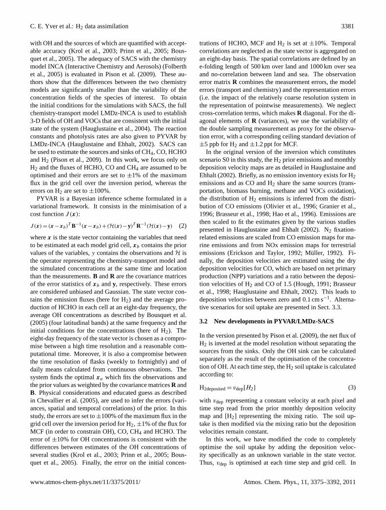
Fig. 4. The three soil deposition velocity maps used in this study. Top: from Hauglustaine and Ehhalt(2002), middle: from Sitch et al. (2003), bottom: from Oslo CTM2 based on Schillert (2010). Whitepixels are missing values.

38

Fig. 4. The three soil deposition velocity maps used in this study. Top: fromHauglustaine and Ehhalt(2002), middle: fromSitch et al.(2003), bottom: from Oslo CTM2 based onSchillert(2010). White pixels are missing values.

Table 3. Scenarios used in this study.

Scenario Model Prior

S0 original settings (H2 net flux inverted) original settings (as inPison et al.(2009)S1 original settings new fluxes and new initial mixing ratiosS2 separate sink new fluxes and new initial mixing ratiosS3 separate sink with LPJ deposition velocity map new fluxes and new initial mixing ratiosS4 separate sink with EUROHYDROS deposition velocity map new fluxes and new initial mixing ratiosS5 separate sink and sources (biomass burning, fossil fuel and others) with

EUROHYDROS deposition velocity mapnew fluxes and new initial mixing ratios

a further attempt to optimise each term of the H2 budget,the sources are also separately inverted. The emissions aresplit into three components: fossil fuel, biomass burning andN2 fixation-related emissions. Prior fossil fuel and biomassburning emissions are inferred from the recent bottom-upCO emission inventory fromLamarque et al.(2010), by ap-plying a mass flux ratio H2/CO of 0.034 and 0.02, respec-tively (Hauglustaine and Ehhalt, 2002; Yver et al., 2009). N2fixation-related emissions remain as they were in the previ-ous version and represent about 25% of the total emissions.The concentrations of HCHO are also optimised using satel-lite measurements from OMI for several 3-D large regions(one scaling factor per 3-D region and per year) as describedin Bousquet et al.(2011).

3.3 Scenarios elaborated for the inversion

Six scenarios have been elaborated (see Table3). In scenarioS0, we invert the net flux of H2 using the emission and de-

position velocity maps fromHauglustaine and Ehhalt(2002)as described previously. The first-guess modelling leads to astrong offset with a simulated mean mixing ratio≈115 ppbhigher than observed.Hauglustaine and Ehhalt(2002) at-tributed this mismatch between model and data to the under-estimation of the soil sink in the Northern Hemisphere duringwinter and spring. Moreover, using the same scenario,Pisonet al. (2009) found an urrealistic accumulation of H2 in theatmosphere attributed partly to the same cause.

In scenario S1, we scale the initial mean mixing ratios tothe observed mean mixing ratios. Moreover, we use updatedprior surface emission fluxes fromLamarque et al.(2010)with H2/CO mass ratio of 0.034 and 0.02 for anthropogenicand biomass burning emissions, respectively (Hauglustaineand Ehhalt, 2002; Yver et al., 2009) and optimised HCHOconcentrations fromBousquet et al.(2011). The depositionvelocity map is scaled by a ratio of 1.28 to take into ac-count the hypothesised underestimation and produce a better



balanced budget assuming that the other terms (production,emission and OH loss) are known and fixed.

In scenarios S2 to S4, the deposition velocity is optimisedseparately from the emissions and for each scenario, a differ-ent prior soil deposition velocity map is used. The S2 depo-sition velocity map is the same as that of S1. A bottom-upsoil uptake estimation calculated by the Lund-Postdam-JenaDynamic Global Vegetation Model (LPJ) (Sitch et al., 2003)yields the map for S3. This model combines process-based,large-scale representations of terrestrial vegetation dynamics(with feedbacks through canopy conductance between photo-synthesis and transpiration) and land-atmosphere carbon andwater exchanges in a modular framework. The H2 soil uptakeis estimated based on the assumption that it is mainly drivenby molecular diffusion. The uptake is then expressed usingFick’s law and depends of the mixing ratio at the surface, thediffusivity of H2 in the soil and the oxidation constant rate.The diffusivity in the soil itself depends of the soil porosityand temperature whereas the oxidation rate depends of soiltemperature, moisture and organic content. This submodelis integrated into the LPJ model. The soil properties arebased on the Food and Agriculture Organization (FAO) dataset overlain by soil organic carbon data from the IGBP-DISdata set (Group, 2000). Soil temperature and moisture aregiven by LPJ. H2 mixing ratio is fixed at 531 ppb. Zero val-ues are applied on oceans and wetlands and when the snowlayer is higher than 50 cm or when the NPP is lower than10 gC m−2 yr−1 (Morfopoulos et al., 2010).

For S4, the monthly map was produced for the EURO-HYDROS project by the Oslo CTM2, an Eulerian chem-ical transport model (Søvde et al., 2008), in combinationwith soil deposition velocities estimated within the projectwith bottom-up and top-down methods compiled inSchillert(2010). Mean values and seasonal cycles are given for threelatitudinal bands: HNH, Tropics and HSH. As the estima-tions for the HSH are sparse, the seasonal cycle in the HSHis the same as in the HNH but shifted of 6 months. The OsloCTM2 couples the ECMWF IFS meteorological data and theMODIS annual L3 global 0.05 Deg landcover map, to EU-ROHYDROS deposition velocities to take into account thelatitudinal distribution and also the effect of snow and wet-lands.

Finally, in scenario S5, surface emissions are further sep-arated into three components: fossil fuel, biomass burningand N2 fixation-related emissions. Scenario S5 uses the priordeposition velocity map from S4.

3.4 Characteristics of the soil deposition velocity maps

As stated in the previous paragraph, we use three differentsoil deposition velocity maps as prior in the model. Thesemaps are shown in Fig.4 for the months of January and July.They present some common large scale features but differfor the magnitude and distribution of regional deposition ve-locity. On a global scale, the highest values are found in

July corresponding to the favorable temperature and mois-ture conditions for high deposition. In January, the maxi-mum values are located in the Southern Hemisphere (australsummer) and in July they are located in the Northern Hemi-sphere except for the S3 map where high deposition veloc-ities are found in the Southern Hemisphere throughout theyear. The first two maps (S0 and S3) are more detailed sincethey are based on vegetation maps. The last one (S4) was cre-ated using deposition velocity measurements combined withthe driving meteorology of the Oslo CTM2. These measure-ments remain sparse and were thus extrapolated to latitudinalbands. The first map (S0) includes the highest grid cell veloc-ities, up to 0.14 cm s−1 in July in the Northern Hemisphere,whereas in the S3 and S4 maps the maximum grid cell depo-sition velocity reaches only 0.07 cm s−1 and 0.06 cm s−1 re-spectively. S0 presents important spatiotemporal variationswith marked hotspots. In the winter, these hotspots are ob-served in Brazil and southern Africa (United Republic ofTanzania, Republic of Mozambique, Zambia and Angola).In summer, hotspots are observed mostly in North Americaand in the north of Russia. These high values are due to thedirect link existing between NPP and deposition velocities inthe assumptions of scenario S0: high NPP produced by favor-able meteorological conditions may lead to too high deposi-tion velocities. In the Southern Hemisphere, these hotspotsreach 0.1 cm s−1 in a grid cell while in the Northern Hemi-sphere, they reach up to 0.14 cm s−1 in a grid cell. InLalloet al.(2008), the highest values found in the boreal forest was0.07 cm s−1 which is about two times lower than the valueshere. These high deposition velocities are then to be consid-ered with caution, as possible artifacts of the use of NPP as aproxy of H2 deposition velocity.

S3 is characterised by the absence of large spatiotemporalvariations. In this map, the deposition velocity is lower northof 30◦ N than south of this latitude (except for the Sahararegion with the desert and Australia).

In S4 map, the latitudinal deposition velocity presentsspatiotemporal variations, but contrary to S0, there are nohotspots. In winter, the larger values are found in SouthAmerica and southern Africa too (Argentina and SouthAfrica). Since the soil uptake is extrapolated from latitudinalbands, there are also large values in southern Australia. Insummer, the higher deposition velocities are observed northof 30◦ N.

Due to the large distribution differences shown in Fig.4,we can expect to find important differences in the first-guesssimulations.

4 Results and discussion

4.1 Evaluation of the first-guess and inverse simulations

In Fig. 5, we present the simulated and observed mixing ra-tios for four sites: the northernmost site, Alert in Alaska, a



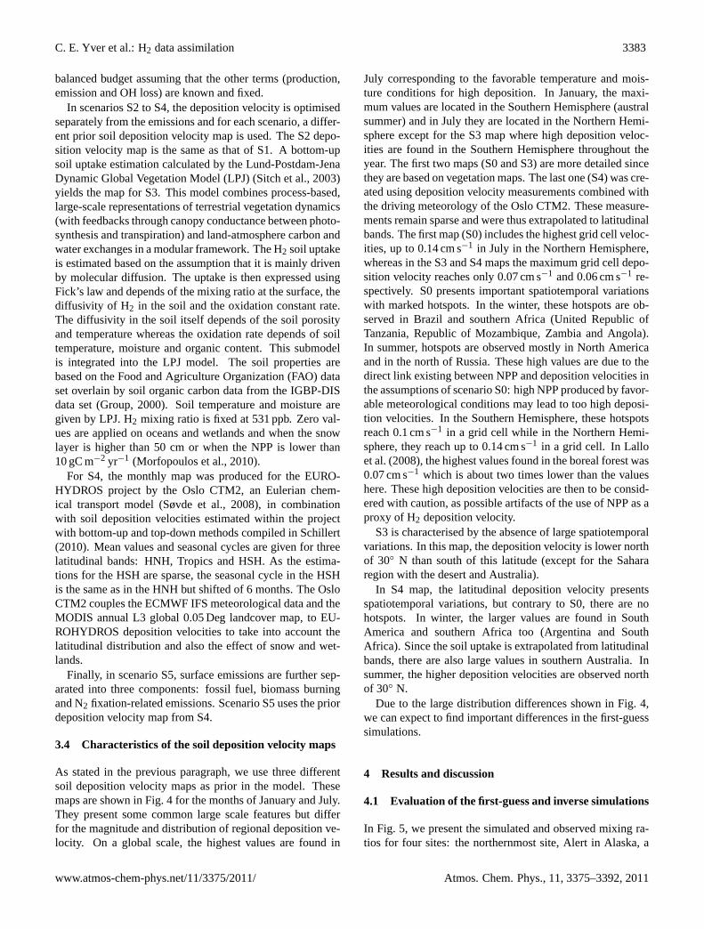
Fig. 5. H2 mixing ratios at Alert, Mace Head, Pondichery and Amsterdam Island. Black filled circlesplot the observations, diamonds, simulated mixing ratios. Each scenario is represented by a differentcolor, S0 and S1 in a red color scale, S2 to S4 in a blue color scale and S5 in green. On the left panel,the prior simulations and on the right panel, the posterior simulations.39

Fig. 5. H2 mixing ratios at Alert, Mace Head, Pondichery and Amsterdam Island. Black filled circles plot the observations, diamonds,simulated mixing ratios. Each scenario is represented by a different color, S0 and S1 in a red color scale, S2 to S4 in a blue color scale andS5 in green. On the left panel, the prior simulations and on the right panel, the posterior simulations.

mid-latitudinal site, Mace Head in Ireland, a northern tropi-cal site, Pondichery in India and a southern hemispheric site,Amsterdam Island. Observations are plotted with black filledcircles. Simulated mixing ratios are plotted in coloured dia-monds with first-guess mixing ratios modelled with the prioremissions on the left panel and inverted mixing ratios on theright panel. As S1 and S2 as well as S4 and S5 use the sameprior information, their first-guess mixing ratios are superim-posed.

As previously mentioned, the first-guess mixing ratiosusing prior emissions from S0 are overestimated by about115 ppb. For the other scenarios, the initial mixing ratioshave been adjusted and the prior fluxes have been updatedso that the mean difference is lower than 40 ppb, except forS3, which presents a mean difference of 87 ppb due to a driftin time as the prior budget is not balanced. At Alert, thefirst-guess simulated seasonal cycle of S0 to S2 follows theobserved cycle with a maximum in autumn and a minimumat the beginning of spring. For S3 through S5, the seasonalcycle is about two months late. At Mace Head, on the con-trary, the first-guess simulated seasonal cycle of S0 to S2 isabout two months in advance, whereas S3, S4 and S5 followthe observed cycle. For the other sites, the weak seasonal cy-cle is well reproduced. The first-guess mixing ratios of S3,S4 and S5 present a qualitatively better agreement with theobserved seasonal cycle at all sites. The seasonal amplitudeis fairly well represented by all of the first-guess simulationsexcept for S3, for which the seasonal amplitude is weaker.

For all sites, the first-guess mixing ratios of S3, S4 and S5present a drift of 50, 30 and 30 ppb yr−1 respectively. This isdue to the fact that the prior H2 budget is not balanced sincewe use different soil deposition maps. We also see a slightdecrease in S0 first-guess mixing ratios for Amsterdam Is-land which is not observed in the measurements.

After inversion, as expected, the simulated mixing ratiosfit the observations better in terms of amplitude as well asseasonal cycle. The mean difference between observationsand simulated mixing ratios is thus close to zero. The meancoefficient of correlation between the observations and thesimulations increases from 0.2 to 0.5. The better correlationfor the scenarios including the separate soil uptake optimisa-tion is found for S4 with a mean difference around−1.5 ppb(+35 ppb for the first-guess), a standard deviation of 17 ppb(47 ppb for the first-guess) and a coefficient of correlation of0.6 (0.4 for the first-guess). S5, where the sources are fur-ther separated, presents very close results (mean difference1.8 ppb, standard deviation 18 ppb and coefficient of correla-tion of 0.6).

4.2 Inverted fluxes

For each process in the H2 budget, the flux interannual vari-ations remain small, below±5 Tg yr−1. All of the scenariosare consistent for the interannual variations in terms of pat-tern and amplitude (not shown). In Fig.6, the mean seasonalcycle for each flux in 2006-2009 is plotted after inversion



Fig. 6. Posterior seasonal cycle of H2 fluxes for four regions (HNH: High North Hemisphere, 30−90◦N;Tropics, between 30◦N and 30◦S; HSH: High Southern Hemisphere, 30−90◦S). Each scenario is rep-resented by a different color, S0 and S1 in red scale, S2 to S4 in blue scale and S5 in green. The prioremissions for the S5 scenario are plotted in light green and labelled S5 fwd. Separated emissions of S5and S5 fwd are plotted with dots for the biomass burning emissions, with dashes for the anthropogenicemissions and with dashes-dots for the N2 fixation-related emissions. The grey shaded area representsthe spread between the different scenarios.

40

Fig. 6. Posterior seasonal cycle of H2 fluxes for four regions (HNH: High North Hemisphere, 30−90◦ N; Tropics, between 30◦ N and 30◦

S; HSH: High Southern Hemisphere, 30–90◦ S). Each scenario is represented by a different color, S0 and S1 in red scale, S2 to S4 in bluescale and S5 in green. The prior emissions for the S5 scenario are plotted in light green and labelled S5 fwd. Separated emissions of S5 andS5 fwd are plotted with dots for the biomass burning emissions, with dashes for the anthropogenic emissions and with dashes-dots for theN2 fixation-related emissions. The grey shaded area represents the spread between the different scenarios.

for all of the scenarios. The prior fluxes of S5 are addedfor comparison. As S4 and S5 differs only by the separationof the sources, the inverted fluxes for the sinks and for theHCHO source are superimposed. For each process, we havestudied three regions: the High Northern Hemisphere (HNH)north of 30◦ N, the Tropics, between 30◦ N and 30◦ S andthe High Southern Hemisphere (HSH) south of 30◦ S. As ex-plained before, H2 photochemical production and OH lossare strongly constrained and therefore, the inverted fluxesstay close to the prior fluxes. The difference of≈5 Tg yr−1

between S0 and the other scenarios for the photochemicalproduction is due to the change of the prior HCHO concen-trations between the first scenario and the others. An errorof ±100% has been assigned to the prior deposition veloc-ity and to the emissions and these ones are therefore moresubject to changes. The soil uptake seasonal cycle presentslarge variations in the HNH. S0 and S1, where the depositionvelocity is not separately inverted, exhibit their maximum inJune. For S2, with the separated inversion of the depositionvelocity, the maximum is shifted to July and for S3, S4 andS5, the maximum is shifted to August. In comparison, thesoil uptake values, obtained with bottom-up and top-downmethods, are maximum at the end of August or the beginningof September (Schillert, 2010). Moreover, the observed mix-ing ratios, which are dominated by the uptake in the HNH,are minimum at the end of summer as well. The shift from

June to August shows that we are able to reproduce the sea-sonal cycle of the soil uptake better than with the previousassumptions. In the Tropics and the HSH, no seasonal cycleis apparent and the mean value is consistent among all of thescenarios.

In S0, it was supposed that the soil sink was too weakin the HNH (Hauglustaine and Ehhalt, 2002) producing anaccumulation of H2 in the atmosphere, so in S1 and S2 wehave increased the prior deposition velocities by 30% to bet-ter balance the budget. In S1, we still invert the net H2 fluxand the soil sink remains nearly the same as the prior flux.In S2, since we separately invert the deposition velocity andthe surface emissions, the deposition velocities are optimisedand the resulting HNH soil uptake is nearly back to the valueof S0. This seems to imply that the soil uptake in S0 wasnot that weak but that the offset between the simulated mix-ing ratios and observations has other causes. Errors in theregional distribution of deposition velocities or in emissionstrength are possible explanation for such an offset.

Overall, the seasonal cycle of the surface emissions peaksin the HNH in June for S0 to S2 and in August for S3 toS5. This can be explained by the change in the seasonal-ity of the soil uptake which shifts from June to August aswell, highlighting the fact that the different processes are notindependently inverted. In the Tropics, two maxima are ob-served, one in March and the second in September. They



coincide with the biomass burning maxima of each hemi-sphere, in March in the south and in August/September inthe north (van der Werf et al., 2006). Bousquet et al.(2011)found two peaks as well, the first one in mid-March and thesecond, which is also the larger one, in September. S2, S4and S5 reproduce this same pattern. The southern maximumis clearly apparent for S1, S2 and S5 but weak for S0, S3and S4. Except for S1, the second maximum in September islarger. We observe a good agreement among all of the sce-narios, except for S0 and S1, for the amplitude of the summerpeak. In the Southern Hemisphere, there are only very smallsurface emissions.

In S5, we have separately inverted the emissions in threedifferent processes. Biomass burning (dark green dots),anthropogenic (dark green dashes) and N2 fixation-related(dark green dashes-dots) emissions are plotted in the samepanel as the total surface emissions. The prior is overplot-ted in light green with the same symbols for each source.The seasonality is mainly driven by the biomass burningemissions whereas the anthropogenic and N2 fixation-relatedemissions are more or less constant throughout the year.

From the analysis of the differences between the observa-tions and the simulated mixing ratios and from the compar-ison of the timing of the modelled soil uptake and biomassburning emissions with the measured fluxes, it can be con-cluded that S5 is the more pertinent scenario. Therefore, thefollowing discussion on the H2 budget focuses on the resultsof this scenario.

4.3 H2 budget

In Table4, the mean estimation for each term of the globaland regional budget is calculated for 2007, 2008 and thewhole period based on scenario S5. The global estimationsfor each term as given inXiao et al. (2007) and Bousquetet al. (2011) are added in Table4. Estimating the uncer-tainties of the posterior fluxes can be done using the Monte-Carlo approach ofChevallier et al.(2007). However, duethe large computational cost of this method, a simpler ap-proach was preferred. The one-sigma uncertainties are esti-mated from the spread of the difference between each sce-nario compared to reference scenario S5 for each flux. Wedo not include S0 because, in this scenario, the prior HCHOflux is ≈5 Tg yr−1 lower than the prior flux in the other sce-narios and, as explained previously, prescribed with smalluncertainties. Moreover, the uncertainties of Table4 do notinclude all sources of uncertainties. For instance, they do notaccount explicitly for transport model errors, for chemistrymodel errors, or for uncertainties in the inversion setup otherthan the distribution of deposition velocities. They shouldtherefore be considered as lower estimates. Performing ananalysis of the full uncertainties associated to the values inTable4 is an important and complex matter which lays be-yond the scope of this work. ForBousquet et al.(2011),we have indicated the standard deviation of the sensitivity

Fig. 7. Posterior H2 budget per process (above) and regions (below). Each colour bar represents ascenario.

41

Fig. 7. Posterior H2 budget per process (above) and regions (be-low). Each colour bar represents a scenario.

inversions based on the reference scenario (external errors).The errors inXiao et al.(2007) include model uncertainties,absolute calibration error and errors in the assumed fossilfuel source strength. For each region, we indicate the rela-tive proportion of each regional source or sink in compari-son with the global source or sink. Figure7 represents thisbudget per process and per region. All of the scenarios pro-duce a consistent process-based view (maximum spread of9.0 Tg yr−1). From a region-based view, the total H2 fluxranges between−8 and+8 Tg yr−1 with a maximum spreadof 4 Tg yr−1 (not shown). For all of the scenarios, the HNHis a net sink of H2 and the Tropics are a net source. Glob-ally, ≈47 Tg yr−1 of H2 are produced by photochemical pro-duction and≈18 Tg yr−1 are consumed by the OH reaction.Approximately 36 Tg yr−1 are emitted and≈59 Tg yr−1 aredeposited in the soils. This budget leads to a troposphericburden of 166 Tg and a life time of 2.2 years. This budget isconsistent with most of the previous studies about H2 cyclesuch asEhhalt and Rohrer(2009) who published a tropo-spheric burden of 155 Tg and a life time of 2.0 years.

Every process has a larger flux in the Tropics than it has inthe HNH or HSH. Tropical processes represent between 55%and 74% of global processes depending on the flux types. In-deed, the photochemical production and the OH sink dependstrongly on insolation which has its maximum in the Tropics.



Table 4. H2 budget per process in Tg yr−1 (∗ in Bousquet et al.(2011) the fossil fuel and N2 fixation related emissions are inverted together).The indicated error represents the maximum spread of the scenarios S1 to S4 compared to S5 for this study, the standard deviation of thesensitivity inversions forBousquet et al.(2011) and forXiao et al.(2007), the model uncertainties, absolute calibration error and errors inthe assumed fossil fuel source strength. The % represent the part of each regional term in the global term. The separated emission terms arenot associated with error in this study as we did not perform several sensitivity tests.

Global 2007 2008 mid 2006−mid 2009

Thisstudy

Bousquetet al.(2011)

Xiaoet al.(2007)

Biomass Burning 7.8 7.7 7.8 10±2 12±3Fossil fuel 18.8 18.3 18.5 22±3∗ 15±10N2 fixation 9.5 9.4 9.4 ∗

−

Emissions 36.0±5.4 35.4±5.5 35.7±4.3 32±5 27±9Photochemical production 46.9±0.1 46.5±0.2 46.5±0.2 48±4 76±13OH loss −18.1±0.5 −18.2±0.4 −18.2±0.4 −18±1 −18±3Soil uptake −58.0±8.6 −59.9±8.6 −58.8±9.0 −62±3 −84±8

North hemisphere 2007 2008 mid 2006−mid 2009

Biomass Burning 1.3 1.3 1.3Fossil fuel 8.3 8.0 8.0N2 fixation 3.7 3.7 3.7Emissions 13.3±1.7 13.0±2.6 13.0±1.7 (36%) 50% 37%Photochemical production 10.7±0.1 10.6±0.1 10.6±0.0 (23%) 33% 17%OH loss −2.9±0.1 −2.9±0.1 −2.9±0.1(16%) 22% 12%Soil uptake −22.5±3.3 −23.8±2.9 −23.3±3.6 (40%) 53% 39%

Tropics 2007 2008 mid 2006-mid 2009

Biomass Burning 6.3 6.3 6.4Fossil fuel 10.2 10.0 10.1N2 fixation 5.1 5.1 5.1Emissions 21.6±3.6 21.3±3.0 21.6±3.0 (61%) 47% 62%Photochemical production 32.2±0.1 31.9±0.1 31.9±0.1 (69%) 38% 75%OH loss −13.4±0.5 −13.4±0.5 −13.4±0.5 (74%) 50% 77%Soil uptake −32.5±4.5 −33.0±4.7 −32.6±4.9 (55%) 18% 55%

South hemisphere 2007 2008 mid 2006-mid 2009

Biomass Burning 0.1 0.1 0.1Fossil fuel 0.4 0.4 0.4N2 fixation 0.6 0.6 0.6Emissions 1.1±0.0 1.1±0.0 1.1±0.0 (3%) 3% 1%Photochemical production 4.1±0.0 4.0±0.0 4.0±0.0 (8%) 29% 8%OH loss −1.9±0.1 −1.9±0.1 −1.9±0.1 (10%) 28% 11%Soil uptake −3.0±0.9 −3.0±0.9 −3.0±0.9 (5%) 29% 6%

The tropical maximum in the surface emissions is due tobiomass burning emissions. For the maximum of soil up-take in the Tropics (55%), asXiao et al.(2007) have alreadyproposed, one explanation could be that the tropical soils aremore efficient in terms of uptake than the extra-tropical soils.It could also be linked to the optimum conditions in the hu-midity and temperature of this region. The soil sink in theHNH nevertheless represents 40% of the global soil sink.

The mean values of the global budget remain, within theuncertainties, compatible with the one presented inBousquetet al.(2011). The budget fromXiao et al.(2007) differs sig-nificantly except for the OH loss. Their emissions are lowerbut their photochemical production and their soil uptake aremore than 20 Tg yr−1 larger than in our work. The distri-bution between the different regions is more consistent withXiao et al.(2007) than withBousquet et al.(2011). This re-sult is explained by the fact that, in our study and inXiaoet al.(2007), the budget was analysed through the same three



Fig. 8. S5 posterior flux map (on the left) and difference between S5 posterior and prior in % of theprior (on the right) fluxes for the surface emissions (above) and soil uptake (below) zoomed on Europefor March, April and May (MAM) and September, October and November (SON). Missing values areplotted in white.

42

Fig. 8. S5 posterior flux map (on the left) and difference betweenS5 posterior and prior in % of the prior (on the right) fluxes forthe surface emissions (above) and soil uptake (below) zoomed onEurope for March, April and May (MAM) and September, Octoberand November (SON). Missing values are plotted in white.

latitudinal bands, whereasBousquet et al.(2011) used largeregions that do not exactly fit these latitudinal bands. Finally,our estimate of biomass burning emissions is of the same or-der of magnitude asBousquet et al.(2011) andXiao et al.(2007) but our estimation represents only 22% of the totalemissions against 31% and 44% forBousquet et al.(2011)andXiao et al.(2007), respectively.

4.4 Focus on Europe

In this study, Europe exhibits the largest number of obser-vation sites, therefore being the best constrained area of theworld for an atmospheric inversion. As seen in Fig.7, Eu-rope, as part of the HNH, seems to be a net sink of H2.In Fig. 8, the posterior flux map and the difference betweenposterior and prior in percentage of the prior for the S5 sur-face emissions and soil uptake are plotted. The emissionsin Europe present the same pattern in the spring and au-tumn. However, in the autumn, the emissions are slightlyhigher (grid cell maximum of 0.8 Tg yr−1) than they are inthe spring (grid cell maximum of 0.5 Tg yr−1). This autumnflux can be explained from the seasonal cycle (see Fig.6), bya combination of enhanced biomass burning and N2 fixation-

related emissions at the end of the summer and a small in-crease of the anthropogenic emissions at the end of the year.The differences between prior and posterior range from−60to 0% in spring and from−15 to +30% in autumn for theemissions. This means that in spring, the inversion reducesEuropean prior emissions, especially in western Europe. Inautumn, western prior emissions are only slightly decreased,but eastern prior emissions are largely increased by the in-version. As expected, the spring soil uptake is smaller thanthe autumn soil uptake especially in the boreal region and thesouth of Europe. The uptake in central Europe, smaller in au-tumn than in summer, may be explained by early snow in thealpine region in autumn. The differences between prior andposterior range from−7 to+35% in spring and from−58 to+10% in autumn. The spring soil uptake is increased in allof Europe compared to the prior estimate. In autumn, a largedecrease of the prior soil uptake is found for northern Eu-rope, whereas western Europe fluxes are increased comparedto the prior.

In Table5, the emissions and the soil uptake are detailedfor seven countries or groups of countries: geographical Eu-rope (including the European part of Russia, west of theUral mountains); Europe (27 countries); France; Germany;the United Kingdom and Ireland; Scandinavia and Finland;Spain, Italy and Portugal. In terms of emissions, geograph-ical Europe represents 6% and 18% of the global and HNHemissions respectively. The European soil uptake accountsfor 7% and 17% of the global and HNH uptake, respec-tively. Anthropogenic emissions account for 52% of the to-tal emissions globally, 62% in the HNH and 72% in Europe(27 countries). In Europe, depending on the countries, an-thropogenic emissions account for 50% to 100% of the totalemissions. As written above, there is no bottom-up inventoryof H2 emissions. We have then compared our results withthe inventory from the Institut fur Energiewirtschaft und Ra-tionelle Energieanwendung (IER) (Thiruchittampalam andKoble, 2004), which is not used as prior information (seeTable5). We have scaled the CO emissions with the anthro-pogenic H2/CO mass ratio of 0.034 as found inYver et al.(2009). The two sets of values agree well with one another.The mean difference lies around 10%. Uncertainties on in-ventories are not yet produced quantitatively but the EDGARdatabase has proposed ranges of uncertainties: low (±10%),medium (±50%) and large (±100%) (Olivier et al., 1996).For CO, most uncertainties by source types are reported as“medium”, therefore making our results consistent with IERestimates, within their respective uncertainties.

5 Conclusions

This work presents the results of an inversion of troposphericH2 sources and sinks at a grid cell resolution for the pe-riod between mid-2006 and mid-2009. It focuses on soil up-take and surface emissions. Overall, the results of this study



Table 5. H2 budget per country in Europe in Tg yr−1. The indicated error represents the maximum spread of the scenarios S1 to S4compared to S5 for the emissions and of the scenarios S2 to S4 compared to S5 for the soil uptake as the soil uptake is not inverted inscenario S1. In bold, the anthropogenic emissions from S5. In italics, the anthropogenic emissions from IER. (Thiruchittampalam andKoble, 2004)

Emissions (Tg yr−1) 2007 2008 mid 2006-mid 2009

Total Anthropogenic Anthropogenic from IEREurope (geographical) 2.2±0.4 2.3±0.6 2.2±0.3 1.4 1.5Europe (27) 1.2±0.3 1.4±0.4 1.3±0.2 0.9 1.0France 0.2±0.1 0.2±0.1 0.2<0.1 0.2 0.2Germany 0.2±0.1 0.2±0.1 0.2±0.1 0.1 0.1UK + Ireland 0.1<0.1 0.1<0.1 0.1<0.1 0.1 0.1Scandinavia + Finland 0.1<0.1 0.1<0.1 0.1<0.1 0.1 0.1Spain+Italy+Portugal 0.3<0.1 0.3<0.1 0.3<0.1 0.2 0.2

Soil uptake (Tg yr−1) 2007 2008 mid 2006-mid 2009

Europe (geographical) −3.9±0.7 −4.0±0.7 −3.9±0.7Europe (27) −1.6±0.3 −1.7±0.3 −1.6±0.3France −0.3<0.1 −0.3<0.1 −0.3<0.1Germany −0.2<0.1 −0.2<0.1 −0.2<0.1UK + Ireland −0.1±0.1 0.0±0.1 −0.1±0.1Scandinavia + Finland −0.3±0.2 −0.4±0.2 −0.3±0.2Spain+Italy+Portugal −0.3±0.2 −0.3±0.2 −0.3±0.2

agree with previous studies with regard to a lifetime of abouttwo years, a soil uptake of≈−59 Tg yr−1 and emissions of≈36 Tg yr−1 for a total source of≈83 Tg yr−1. The inver-sions performed from six different scenarios are fairly con-sistent with one another in terms of physical processes in-volved (maximum spread of 9 Tg yr−1) and of flux location(maximum spread of 4 Tg yr−1). From the several scenariosthat have been elaborated, the best one (S5) in terms of fit tothe mean atmospheric mixing ratio, seasonal cycle and fluxmeasurements combines a separate inversion of the soil sinkand of the sources in three terms and a soil deposition veloc-ity map based on soil uptake measurements. Our estimationfor the global soil uptake is−59±9 Tg yr−1. 95% of thisuptake is located in the HNH (40%) and the Tropics (55%).No significant trend is found for the soil uptake or any of theother processes of the H2 budget throughout 2006−2009. Tostudy the emissions better, scenario S5 with a separate in-version of the sources in three processes (biomass burning,fossil fuel and N2 fixation-related emissions) shows that theseasonal variability of the emissions is mainly driven by thebiomass burning emissions. Finally, we have focused ouranalysis on Europe and compared the anthropogenic emis-sions with a CO inventory scaled with a H2/CO mass ratio of0.034. Anthropogenic emissions represent 50% to 100% ofthe total emissions depending on the country. The model andthe inventory estimates agree with one another within theirrespective uncertainties. A further step will be to invert otherrelevant species with H2 such as CH4, CO and HCHO, whichis a unique capability of our multispecies inversion system(Pison et al., 2009). In particular, the optimisation of the

HCHO 3-D production, which is fixed in this work, wouldhave an important influence on the H2 budget through theprocess of photochemical production. Performing an anal-ysis of the full uncertainties associated to each term of thebudget will be an important but complex further step.

Future inversions of H2 sources and sinks should gainrobustness by including observations of other networks butalso by including observations of the deuterium enrichmentof H2 (δD of H2), as shown inRhee et al.(2006); Priceet al. (2007). Several groups have producedδD observa-tions (Gerst and Quay, 2001; Rahn et al., 2003; Rockmannet al., 2003; Rhee et al., 2006; Price et al., 2007). Within theEUROHYDROS project,δD observations from six samplingsites are available for the recent years (from 2006). The iso-topic signatures for fossil fuel, biofuel, biomass burning, andocean sources are all depleted in D relative to the atmosphere,whereas photochemical production of H2 has a large positiveisotopic signature. On the sink side, the isotopic fractiona-tion during OH loss is greater than the fractionnation fromsoil uptake (Price et al., 2007). The troposphericδD is about+130±4% (Gerst and Quay, 2000). AssimilatingδD obser-vations together with H2 observations could bring new con-straints on H2 budget if the different isotopic signatures canbe determined with sufficient precision.

Acknowledgements.We gratefully thank Mathilde Grand andVincent Bazantay for performing the flasks and in-situ analysesfor the RAMCES network as well as the people involved in thesamplings and analyses for the EUROHYDROS network. Thankyou to the computing support team of the LSCE. This work wascarried out under the auspices of the 6th EU framework program



# FP6-2005-Global-4 “EUROHYDROS- A European Network forAtmospheric Hydrogen Observations and Studies”. RAMCES isfunded by INSU and CEA.

Edited by: M. Heimann

The publication of this article is financed by CNRS-INSU.

References

Aalto, T., Lallo, M., Hatakka, J., and Laurila, T.: Atmospheric hy-drogen variations and traffic emissions at an urban site in Fin-land, Atmos. Chem. Phys., 9, 7387–7396,doi:10.5194/acp-9-7387-2009, 2009.

Bonasoni, P., Calzolari, F., Colombo, T., Corazza, E., Santaguida,R., and Tesi, G.: Continuous CO and H2 measurements at Mt.Cimone (Italy): Preliminary results, Atmos. Environ., 31, 959–967, 1997.

Bond, S., Vollmer, M., Steinbacher, M., Henne, S., and Reimann,S.: Atmospheric molecular hydrogen (H2): Observations at thehigh-altitude site Jungfraujoch, Switzerland, Tellus, 61B, 64–76,doi:10.1111/j.1600-0889.2010.00509.x, 2010.

Bousquet, P., Hauglustaine, D. A., Peylin, P., Carouge, C., andCiais, P.: Two decades of OH variability as inferred by an in-version of atmospheric transport and chemistry of methyl chlo-roform, Atmos. Chem. Phys., 5, 2635–2656,doi:10.5194/acp-5-2635-2005, 2005.

Bousquet, P., Yver, C., Pison, I., Li, Y. S., Fortems, A., Hauglus-taine, D., Szopa, S., Rayner, P. J., Novelli, P., Langenfelds, R.,Steele, P., Ramonet, M., Schmidt, M., Foster, P., Morfopou-los, C., and Ciais, P.: A three-dimensional synthesis inver-sion of the molecular hydrogen cycle: Sources and sinks bud-get and implications for the soil uptake, J. Geophys. Res., 116,doi:201110.1029/2010JD014599, 2011.

Brasseur, G. P., Hauglustaine, D. A., Walters, S., Rasch, P. J.,Muller, J., Granier, C., and Tie, X. X.: MOZART, a global chem-ical transport model for ozone and related chemical tracers 1.Model description, J. Geophys. Res., 103, 28265–28290, 1998.

Chevallier, F., Fisher, M., Peylin, P., Serrar, S., Bousquet,P., Breon, F., Chedin, A., and Ciais, P.: Inferring CO2sources and sinks from satellite observations: Method andapplication to TOVS data, J. Geophys. Res., 110, D24309,doi:10.1029/2005JD006390, 2005.

Chevallier, F., Breon, F., and Rayner, P. J.: Contributionof the Orbiting Carbon Observatory to the estimation ofCO2 sources and sinks: Theoretical study in a variationaldata assimilation framework, J. Geophys. Res., 112, 11 pp.,doi:200710.1029/2006JD007375, 2007.

Conrad, R. and Seiler, W.: Decomposition of Atmospheric Hy-drogen By Soil Microorganisms and Soil Enzymes., Soil Biol.Biochem., 13, 43–49, 1981.

Conrad, R. and Seiler, W.: Influence of temperature, moisture, andorganic carbon on the flux of H2 and CO between soil and at-mosphere: Field studies in subtropical regions, J. Geophys. Res.,90, 5699–5709, 1985.

Ehhalt, D. H. and Rohrer, F.: The tropospheric cycle of H2: A crit-ical review, Tellus, 61B, 500–535, 2009.

Engel, A. and EUROHYDROS PIs: EUROHYDROS, A EuropeanNetwork for Atmospheric Hydrogen observations and studies.,in: EUROHYDROS Final Report,http://cordis.europa.eu/, 2009.

Erickson, D. J. and Taylor, J. A.: 3-D tropospheric CO modeling- The possible influence of the ocean, Geophys. Res. Lett., 19,1955–1958, 1992.

Folberth, G., Hauglustaine, D. A., Ciais, P., and Lathiere, J.: On therole of atmospheric chemistry in the global CO 2 budget, Geo-phys. Res. Lett, 32, L0881, doi:10.1029/2004GL021812, 2005.

Gerst, S. and Quay, P.: The deuterium content of atmosphericmolecular hydrogen: Method and initial measurements, J. Geo-phys. Res., 105, 26433–26446, 2000.

Gerst, S. and Quay, P.: Deuterium component of the global molec-ular hydrogen cycle, J. Geophys. Res., 106, 5021–5029, 2001.

Granier, C., Hao, W. M., Brasseur, G., and Muller, J.-F.: Land usepractices and biomass burning: Impact on the chemical composi-tion of the atmosphere, in Biomass Burning and Global Change,edited by: Levine, J. S., MIT Press, Cambridge, Mass., USA,140–148, 1996.

Grant, A., Witham, C., Simmonds, P., Manning, A., and O’Doherty,S.: A 15 year record of high-frequency, in situ measurements ofhydrogen at Mace Head, Ireland, Atmos. Chem. Phys., 10, 1203–1214,doi:10.5194/acp-10-1203-2010, 2010.

Group, G. S. D. T.: Global Gridded Surfaces of Selected Soil Char-acteristics (IGBP-DIS). Data set, Oak Ridge National LaboratoryDistributed Active Archive Center, Oak Ridge, Tennessee, USA,http://www.daac.ornl.gov, 2000.

Hammer, S. and Levin, I.: Seasonal variation of the molecular hy-drogen uptake by soils inferred from continuous atmospheric ob-servations in Heidelberg, southwest Germany, Tellus, 61B, 556–565, 2009.

Hammer, S., Vogel, F., Kaul, M., and Levin, I.: The H2/CO ra-tio of emissions from combustion sources: comparison of top-down with bottom-up measurements in southwest Germany, Tel-lus, 61B, 547–555, 2009.

Hao, W. M., Ward, D. E., Olbu, G., and Baker, S. P.: Emissionsof CO2, CO, and hydrocarbons from fires in diverse African sa-vanna ecosystems, J. Geophys. Res., 101, 23577–23584, 1996.

Hauglustaine, D. A. and Ehhalt, D. H.: A three-dimensional modelof molecular hydrogen in the troposphere, J. Geophys. Res., 107,4330, doi:10.1029/2001JD001156, 2002.

Hauglustaine, D. A., Hourdin, F., Jourdain, L., Filiberti, M. A.,Walters, S., Lamarque, J. F., and Holland, E. A.: Interac-tive chemistry in the Laboratoire de Meteorologie Dynamiquegeneral circulation model: Description and background tropo-spheric chemistry evaluation, J. Geophys. Res., 109, D04314,doi:10.1029/2003JD003957, 2004.

Hough, A. M.: Development of a Two-Dimensional Global Tropo-spheric Model: Model Chemistry, J. Geophys. Res., 96, 7325–7362, 1991.

Hourdin, F. and Talagrand, O.: Eulerian backtracking of atmo-spheric tracers. I: Adjoint derivation and parametrization ofsubgrid-scale transport, Quarterly J. Roy. Meteorol. Soc., 132,


http://dx.doi.org/10.5194/acp-9-7387-2009




http://cordis.europa.eu/


http://www.daac.ornl.gov


567–583, 2006.Hourdin, F., Musat, I., Bony, S., Braconnot, P., Codron, F.,

Dufresne, J., Fairhead, L., Filiberti, M., Friedlingstein, P., Grand-peix, J., Krinner, G., LeVan, P., Li, Z., and Lott, F.: The LMDZ4general circulation model: climate performance and sensitivityto parametrized physics with emphasis on tropical convection,Clim. Dynam., 27, 787–813, 2006.

Jordan, A. and Steinberg, B.: Calibration of atmospheric hy-drogen measurements, Atmos. Meas. Tech., 4, 509–521,doi:10.5194/amt-4-509-2011, 2011.

Kaminski, T., Rayner, P. J., Heimann, M., and Enting, I. G.: On ag-gregation errors in atmospheric transport inversions, J. Geophys.Res., 106, 4703–4715, doi:200110.1029/2000JD900581, 2000.

Khalil, M. A. K. and Rasmussen, R. A.: Global increase of atmo-spheric molecular hydrogen, Nature, 347, 743–745, 1990.

Krol, M. C., Lelieveld, J., Oram, D. E., Sturrock, G. A., Penkett,S. A., Brenninkmeijer, C. A. M., Gros, V., Williams, J., andScheeren, H. A.: Continuing emissions of methyl chloroformfrom Europe, Nature, 421, 131–135, 2003.

Lallo, M., Aalto, T., Laurila, T., and Hatakka, J.: Sea-sonal variations in hydrogen deposition to boreal forestsoil in southern Finland, Geophys. Res. Lett., 35, L04402,doi:10.1029/2007GL032357, 2008.

Lallo, M., Aalto, T., Hatakka, J., and Laurila, T.: Hydrogen soildeposition at an urban site in Finland, Atmos. Chem. Phys., 9,8559–8571,doi:10.5194/acp-9-8559-2009, 2009.

Lamarque, J.-F., Bond, T. C., Eyring, V., Granier, C., Heil, A.,Klimont, Z., Lee, D., Liousse, C., Mieville, A., Owen, B.,Schultz, M. G., Shindell, D., Smith, S. J., Stehfest, E., VanAardenne, J., Cooper, O. R., Kainuma, M., Mahowald, N., Mc-Connell, J. R., Naik, V., Riahi, K., and van Vuuren, D. P.: His-torical (1850-2000) gridded anthropogenic and biomass burningemissions of reactive gases and aerosols: methodology and ap-plication, Atmos. Chem. Phys., 10, 7017–7039,doi:10.5194/acp-10-7017-2010, 2010.

Langenfelds, R. L., Francey, R. J., Pak, B. C., Steele, L. P., Lloyd,J., Trudinger, C. M., and Allison, C. E.: Interannual growth ratevariations of atmospheric CO 2 and itsδ13C, H2, CH4, and CObetween 1992 and 1999 linked to biomass burning, Global Bio-geochem. Cy., 16, 1048, doi:10.1029/2001GB001466, 2002.

Morfopoulos, C., Foster, P., Friedlingstein, P., Bousquet, P., andPrentice, I.: Modelling the soil consumption of atmospheric hy-drogen at a global scale, Global Biogeochem. Cy., submitted,2010.

Muller, J.: Geographical Distribution and Seasonal Variation of Sur-face Emissions and Deposition Velocities of Atmospheric TraceGases, J. Geophys. Res., 97, 3787–3804, 1992.

Novelli, P. C., Lang, P. M., Masarie, K. A., Hurst, D. F., Myers,R., and Elkins, J. W.: Molecular hydrogen in the troposphere-Global distribution and budget, J. Geophys. Res., 104, 30427–30444, 1999.

Olivier, J. G. J., Bouwman, A. F., van der Maas, C. W. M.,Berdowski, J. J. M., Veldt, C., Bloos, J. P. J., Visschedijk, A.J. H., Zandveld, P. Y. J., and Haverlag, J. L.: Description ofEDGAR Version 2.0: A set of global emission inventories ofgreenhouse gases and ozone-depleting substances for all anthro-pogenic and most natural sources on a per country basis and on 1degree× 1 degree grid, Rijksinstituut voor Volksgezondheid enMilieu RIVM, 1996.

Pison, I., Bousquet, P., Chevallier, F., Szopa, S., and Hauglus-taine, D.: Multi-species inversion of CH4, CO and H2 emissionsfrom surface measurements, Atmos. Chem. Phys., 9, 5281–5297,doi:10.5194/acp-9-5281-2009, 2009.

Price, H., Jaegle, L., Rice, A., Quay, P., Novelli, P. C., andGammon, R.: Global budget of molecular hydrogen and itsdeuterium content: Constraints from ground station, cruise,and aircraft observations, J. Geophys. Res., 112, D22108,doi:10.1029/2006JD008152, 2007.

Prinn, R. G., Weiss, R. F., Fraser, P. J., Simmonds, P. G., Cunnold,D. M., Alyea, F. N., O’Doherty, S., Salameh, P., Miller, B. R.,Huang, J., Wang, R. H. J., Hartley, D. E., Harth, C., Steele, L. P.,Sturrock, G., Midgley, P. M., and McCulloch, A.: A history ofchemically and radiatively important gases in air deduced fromALE/GAGE/AGAGE, J. Geophys. Res., 105, 751–792, 2000.

Prinn, R. G., Huang, J., Weiss, R. F., Cunnold, D. M., Fraser, P. J.,Simmonds, P. G., McCulloch, A., Harth, C., Reimann, S., andSalameh, P.: Evidence for variability of atmospheric hydroxylradicals over the past quarter century, Geophys. Res. Lett., 32,L07809, doi:10.1029/2004GL022228, 2005.

Rahn, T., Eiler, J. M., Boering, K. A., Wennberg, P. O., McCarthy,M. C., Tyler, S., Schauffler, S., Donnelly, S., and Atlas, E.: Ex-treme deuterium enrichment in stratospheric hydrogen and theglobal atmospheric budget of H2, Nature, 424, 918–921, 2003.

Rhee, T. S., Brenninkmeijer, C. A. M., and Rockmann, T.: Theoverwhelming role of soils in the global atmospheric hydrogencycle, Atmos. Chem. Phys., 6, 1611–1625,doi:10.5194/acp-6-1611-2006, 2006.

Rockmann, T., Rhee, T. S., and Engel, A.: Heavy hydro-gen in the stratosphere, Atmos. Chem. Phys., 3, 2015–2023,doi:10.5194/acp-3-2015-2003, 2003.

Sanderson, M. G., Collins, W. J., Derwent, R. G., and Johnson,C. E.: Simulation of Global Hydrogen Levels Using a La-grangian Three-Dimensional Model, J. Atmos. Chem., 46, 15–28, 2003.

Schillert, A.: Parameters influencing the seasonality of H2 uptakein soils., State Examination Thesis, 2010.

Schmidt, U.: The latitudinal and vertical distribution of molecu-lar hydrogen in the troposphere, J. Geophys. Res., 83, 941–946,1978.

Schmitt, S., Hanselmann, A., Wollschlager, U., Hammer, S., andLevin, I.: Investigation of parameters controlling the soil sink ofatmospheric molecular hydrogen, Tellus, 61B, 416–423, 2009.

Sitch, S., Smith, B., Prentice, I. C., Arneth, A., Bondeau, A.,Cramer, W., Kaplan, J. O., Levis, S., Lucht, W., Sykes, M. T.,Thonicke, K., and Venevsky, S.: Evaluation of ecosystem dy-namics, plant geography and terrestrial carbon cycling in the LPJdynamic global vegetation model, Global Change Biol., 9, 161–185, 2003.

Søvde, O. A., Gauss, M., Smyshlyaev, S. P., and Isaksen, I. S. A.:Evaluation of the chemical transport model Oslo CTM2 withfocus on arctic winter ozone depletion, J. Geophys. Res., 113,D09304, doi:10.1029/2007JD009240, 2008.

Thiruchittampalam, B. and Koble, R.: European emissionsmap, Institut fur Energiewirtschaft und Rationelle Energiean-wendung(IER); University of Stuttgart,http://carboeurope.ier.uni-stuttgart.de/, 2004.

van der Werf, G. R., Randerson, J. T., Giglio, L., Collatz, G. J.,Kasibhatla, P. S., and Arellano, A. F.: Interannual variability


http://dx.doi.org/10.5194/amt-4-509-2011








http://carboeurope.ier.uni-stuttgart.de/

http://carboeurope.ier.uni-stuttgart.de/


in global biomass burning emissions from 1997 to 2004, At-mos. Chem. Phys., 6, 3423–3441,doi:10.5194/acp-6-3423-2006,2006.

Xiao, X., Prinn, R., Simmonds, P., Steele, L., Novelli, P., Huang,J., Langenfelds, R., O’Doherty, S., Krummel, P., and Fraser,P.: Optimal estimation of the soil uptake rate of molecular hy-drogen from the Advanced Global Atmospheric Gases Experi-ment and other measurements, J. Geophys. Res., 112, D07303,doi:10.1029/2006JD007241, 2007.

Yonemura, S., Kawashima, S., and Tsuruta, H.: Continuous mea-surements of CO and H2 deposition velocities onto an andisol:uptake control by soil moisture, Tellus B – Chem. Phys. Meteo-rol. B, 51, 688–700, 1999.

Yonemura, S., Kawashima, S., and Tsuruta, H.: Carbon monoxide,hydrogen, and methane uptake by soils in a temperate arable fieldand a forest, J. Geophys. Res., 105, 14347–14362, 2000a.

Yonemura, S., Yokozawa, M., Kawashima, S., and Tsuruta, H.:Model Analysis of the Influence of Gas Diffusivity in Soil onCo and H2 Uptake, Tellus, 52B, 919–933, 2000b.

Yver, C., Schmidt, M., Bousquet, P., Zahorowski, W., andRamonet, M.: Estimation of the molecular hydrogen soiluptake and traffic emissions at a suburban site near Paristhrough hydrogen, carbon monoxide, and radon-222 semicon-tinuous measurements, J. Geophys. Res.-Atmos., 114, D18304,doi:10.1029/2009JD012122, 2009.



a new estimation of the recent tropospheric molecular ... · 3376 c. e. yver et al.: h2 data...

Documents