a new control volume ﬁnite element method for the stable ... · pdf fileaccurate solution of...

INTERNATIONAL JOURNAL FOR NUMERICAL METHODS IN ENGINEERINGInt. J. Numer. Meth. Engng 2012; 00:1–23Published online in Wiley InterScience (www.interscience.wiley.com). DOI: 10.1002/nme

A new control volume finite element method for the stable andaccurate solution of the drift-diffusion equations on general

unstructured grids.

Pavel Bochev∗† and Kara Peterson

Numerical Analysis and Applications, MS1320, Sandia National Laboratories,P.O. Box 5800, Albuquerque, New Mexico 87185

SUMMARY

We present a new Control Volume Finite Element Method (CVFEM) for the drift-diffusion equations. Themethod combines a conservative formulation of the current continuity equations with a novel definitionof an exponentially fitted elemental current density. An edge element representation of the nodal CVFEMcurrent density in the diffusive limit motivates this definition. We prove that in the absence of carrier driftthe nodal current is sum of edge currents, which solve one-dimensional diffusion problems, times H(curl)-conforming edge basis functions. Replacement of the edge diffusion problems by one-dimensional drift-diffusion equations extends this representation to the general case. The resulting H(curl,Ω)-conforming,exponentially fitted current (EFC) density field combines the upwind effect from all edges and enablesaccurate computation of current density integrals on arbitrary surfaces inside the elements. This obviatesthe need for the control volumes to be topologically dual to the finite elements and results in a methodthat is stable and accurate on general unstructured finite element grids. This sets apart our approach fromother schemes, such as the Scharfetter-Gummel Box Integration Method, which require topologically dualgrids. Numerical studies of the CVFEM-EFC for a suite of standard advection-diffusion test problems onnonuniform grids confirms the accuracy and the robustness of the new formulation. Simulation of an n-channel MOSFET device tests the method in a more realistic setting. Copyright c© 2012 John Wiley &Sons, Ltd.

Received . . .

KEY WORDS: Control Volume Finite Element method, edge elements, exact sequence, compatiblefinite elements, drift-diffusion equations, device modeling, Scharfetter-Gummel method,topologically dual grids

1. INTRODUCTION

The drift-diffusion equations are a coupled system of nonlinear Partial Differential Equations(PDE’s) [21, 19], which model the motion of electrons and holes in semiconductor materials.Predictive simulation of semiconductor devices depends on the robust, accurate and efficientnumerical solution of these equations. Two desirable properties of numerical schemes for the drift-diffusion equations are (a) stability in the advection-dominated regime, i.e., when charge driftvelocities dominate their diffusivity, and (b) local conservation of electron and hole current densities.

A standard approach for stabilization of advection-dominated problems is to introduce additionaldissipation into the numerical scheme through artificial diffusion, upwinding or exponential fitting.

∗Correspondence to: Numerical Analysis and Applications, MS1320, Sandia National Laboratories, P.O. Box 5800,Albuquerque, New Mexico 87185†Sandia National Laboratories is a multi-program laboratory managed and operated by Sandia Corporation, a whollyowned subsidiary of Lockheed Martin Corporation, for the U.S. Department of Energys National Nuclear SecurityAdministration under contract DE-AC04-94AL85000.

Copyright c© 2012 John Wiley & Sons, Ltd.Prepared using nmeauth.cls [Version: 2010/05/13 v3.00]

2 P. BOCHEV AND K. PETERSON

The development of the exponentially fitted Scharfetter-Gummel (SG) scheme [25] was a majorbreakthrough that enabled stable and accurate numerical solution of the drift-diffusion equations inone-dimension. Extension of SG to multiple dimensions [16, 12, 26] typically relies on topologicallydual grids†; see the right plot in Fig. 1. For such grids, the area of the dual (control volume) sidetimes the SG edge current on the primal edge crossing that side gives an accurate approximationof the current density flux through the boundary of the dual cell. The resulting SG-BIM (BoxIntegration Method, or Finite Boxes approach) scheme has excellent stability and is the workhorsein most modern device simulators [9, 15, 12].

Insofar as conservation of current density is concerned, finite volume and finite element methodsfollow different paths. The former integrate the continuity equation on the (topologically dual)control volumes and apply the Divergence Theorem to transform the volume integrals into surfaceintegrals. This ensures conservation of current density with respect to the dual control volumes.On the other hand, conservative finite elements approximate the current density by div-conformingface elements [6]. The resulting mixed finite element methods [5] have indefinite systems withmore variables than primal Galerkin methods, which approximate only the charge density. However,primal Galerkin methods do not conserve current density and so, they lack one of the two desirableproperties for device simulations.

The Control Volume Finite Element Method (CVFEM) [3] is an alternative approach thatcombines the simplicity of the primal Galerkin method with the local conservation propertiesof finite volume methods, without requiring topologically dual grids. The CVFEM approximatescharge densities using the same nodal shape functions as the primal Galerkin method. However, the“weak” CVFEM equations result from application of the Divergence Theorem to control volumessurrounding the element vertices, i.e., they resemble finite volume equations.

While the CVFEM is conservative, it still needs some form of stabilization for advection-dominated problems [20, 28, 29]. In this paper we present a new CVFEM for the drift-diffusionequations, which uses exponentially fitted H(curl)-conforming currents (CVFEM-EFC) to mergethe exceptional stability of the SG-BIM with the greater flexibility of CVFEM. In a nutshell, wesolve one-dimensional drift-diffusion equations on the edges of the finite element mesh and thenuse H(curl)-conforming edge elements [23] to expand the resulting edge current densities into anelemental current density. In so doing we obtain a method that is essentially equivalent to SG-BIMon topologically dual grids, yet remains robust and accurate in the absence of this property, becausethe elemental current field can be integrated accurately on arbitrary surfaces inside the elements.Computational studies on non-uniform grids using a suite of standard test problems and a morerealistic n-channel metal-oxide semiconductor field-effect transistor (MOSFET) device confirm this.

To motivate our approach we examine the nodal CVFEM currents in the pure diffusion limit.Using the fact that nodal and edge elements are part of an exact sequence we prove that in theabsence of carrier drift the nodal current is sum of edge currents from one-dimensional diffusionproblems times H(curl)-conforming edge basis functions. Therefore, the exponentially fittedH(curl)-conforming current in this paper represents a consistent extension of the nodal currentdensity.

The use of H(curl)-conforming elements to extend edge currents into an elemental currentdensity, and independence from explicit stabilization parameters differentiate the CVFEM-EFCfrom other stabilized CVFEM formulations [29, 28]. These papers stabilize the CVFEM using thesame perturbation functions as the SUPG method [8]. The resulting CVFEMs inherit the SUPGstabilization parameter and the quality of their solutions depends critically on the choice of thisparameter. Finding the optimal stabilization parameter for a given PDE configuration remains an

†We remind the reader that two grids in d-dimensions are topologically dual if there is one-to-one correspondencebetween their k and d− k-dimensional entities. For example, in three dimensions (d = 3) every primal vertex (k = 0)corresponds to a unique dual cell (3− 0 = 3); every primal edge (k = 1) corresponds to a unique dual face (3− 1 = 2),every primal face (k = 2) corresponds to a unique dual edge (3− 2 = 1), and every primal cell (k = 3) correspondsto a unique dual vertex (3− 3 = 0). In two dimensions (d = 2) the correspondence is between primal vertices (k = 0)and dual cells (2− 0 = 2), primal sides (k = 1) and dual sides (2− 1 = 1) and primal cells (k = 2) and dual vertices(2− 2 = 0).

Copyright c© 2012 John Wiley & Sons, Ltd. Int. J. Numer. Meth. Engng (2012)Prepared using nmeauth.cls DOI: 10.1002/nme

CVFEM FOR THE DRIFT-DIFFUSION EQUATIONS 3

open problem. Some of the parameters that enter its definition are not known exactly [13], anddifferent solution features, such as internal discontinuities and boundary layers, require differentdefinitions of this parameter [14].

Our brief survey deliberately omits approaches which use the primal Galerkin formulation ofthe drift-diffusion equations because it lacks the second desirable property, i.e., the local currentconservation. We refer the interested readers to [27] (extension of SUPG to drift-diffusion),[1, 24, 32, 31] (exponentially fitted conforming finite elements), and [30] (stabilized GeneralizedFinite Element) for examples and further details. Likewise, we skip mixed methods for drift-diffusion because of their more complicated computational structure, which does not allow simplereuse of an existing primal Galerkin code infrastructure. We refer to [6, 7] for more informationabout these methods.

The rest of this section reviews the relevant notation and the model drift-diffusion equations. Thecore of this paper is Section 2 where we motivate and define the CVFEM-EFC formulation. Section3 briefly discusses implementation of the method and Section 4 uses Cartesian grids to shed somelight on the distinctions between CVFEM-EFC and SG-BIM. Section 5 presents numerical resultsand Section 6 summarizes our conclusions.

1.1. Notation

In this paper Ω is a bounded region in <n, n = 2, 3 with Lipschitz-continuous boundary ∂Ω. TheNeumann and Dirichlet parts of the boundary are ΓN and ΓD, respectively. We use the standardnotation H1(Ω) for the Sobolev space of order one, L2(Ω) for the space of all square integrablefunctions, and H(curl,Ω) for the space of all square integrable vector fields whose curl is alsosquare integrable. Lower case Roman and Greek letters denote scalar quantities and bold facesymbols are vector quantities. The meaning of the symbol | · | varies with the context and can beEuclidean length, domain measure, or cardinality of a finite set.

Throughout the paper Kh(Ω) is a conforming finite element partition of Ω into elements Ks withsize hs and barycenter bs. The average element size in Kh(Ω) is h > 0. The vertices of the meshare vi and eij is a mesh edge with endpoints vi and vj . The midpoint and the length of eij are

mij =vi + vj

2and hij = |vi − vj | ,

respectively. The vertices, edges, sides, and elements intersecting with entity Ξ are V (Ξ), E(Ξ),S(Ξ), and K(Ξ), respectively. For example, V (Ω) is the set of all mesh vertices, E(Ω) is theset of all mesh edges, V (Ks) are the vertices of element Ks, E(vi) are all edges having vi as avertex, K(eij) are the elements sharing eij , and so on. Note that in two-dimensions E(Ξ) = S(Ξ).Selection of vertex ordering induces orientation of eij ∈ E(Ω):

σij =

−1 if vi is the first vertex of eij , i.e., the vertex order is vi → vj

1 if vi is the second vertex of eij , i.e., the vertex order is vi ← vj(1)

The unit tangent on eij follows the edge orientation

tij = σijvi − vj|vi − vj |

,

and always points towards the second vertex of the edge.We refer to Fig. 1 for a representative control volume Ci associated with vertex vi on an

unstructured grid. The set of all control volumes forms a dual grid K ′h(Ω) with dual vertices V ′,dual edgesE′(Ω), and dual sides S′(Ω). Every primal edge eij corresponds to a dual control volumeside ∂Cij , which is comprised of facets ∂Csij = ∂Cij ∩Ks, ∀Ks ∈ K(eij) that is,

∂Cij =⋃

Ks∈K(eij)

∂Csij .



Ci!

Ks!

br!

eij!

vi!

vj!

Kt!

vk!

mik!

mil!vl!

bt!

vm!

Kr! Ku!bu!

bs!

!

"Cijs

!

"Cijt

mim!!

mijt

!

mijs

tik! Ci!

Ks!

br!

eij!

vi!

vj!Kt!

vk!

mik!

mil!

vl!

bt!

vm!

Kr! Ku!

bu!

bs!

mim!!

"Cij

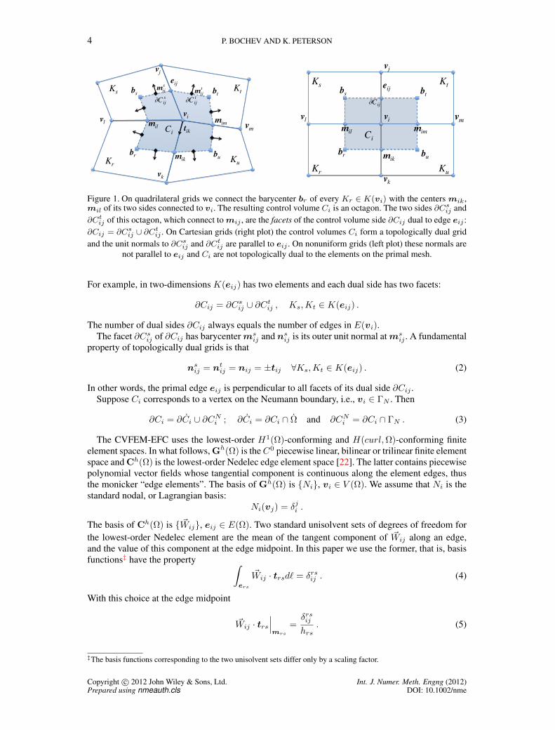
Figure 1. On quadrilateral grids we connect the barycenter br of every Kr ∈ K(vi) with the centers mik,mil of its two sides connected to vi. The resulting control volume Ci is an octagon. The two sides ∂Csij and∂Ctij of this octagon, which connect to mij , are the facets of the control volume side ∂Cij dual to edge eij :∂Cij = ∂Csij ∪ ∂C

tij . On Cartesian grids (right plot) the control volumes Ci form a topologically dual grid

and the unit normals to ∂Csij and ∂Ctij are parallel to eij . On nonuniform grids (left plot) these normals arenot parallel to eij and Ci are not topologically dual to the elements on the primal mesh.

For example, in two-dimensions K(eij) has two elements and each dual side has two facets:

∂Cij = ∂Csij ∪ ∂Ctij , Ks,Kt ∈ K(eij) .

The number of dual sides ∂Cij always equals the number of edges in E(vi).The facet ∂Csij of ∂Cij has barycenter ms

ij and nsij is its outer unit normal at msij . A fundamental

property of topologically dual grids is that

nsij = ntij = nij = ±tij ∀Ks,Kt ∈ K(eij) . (2)

In other words, the primal edge eij is perpendicular to all facets of its dual side ∂Cij .Suppose Ci corresponds to a vertex on the Neumann boundary, i.e., vi ∈ ΓN . Then

∂Ci = ∂Ci ∪ ∂CNi ; ∂Ci = ∂Ci ∩ Ω and ∂CNi = ∂Ci ∩ ΓN . (3)

The CVFEM-EFC uses the lowest-order H1(Ω)-conforming and H(curl,Ω)-conforming finiteelement spaces. In what follows, Gh(Ω) is theC0 piecewise linear, bilinear or trilinear finite elementspace and Ch(Ω) is the lowest-order Nedelec edge element space [22]. The latter contains piecewisepolynomial vector fields whose tangential component is continuous along the element edges, thusthe monicker “edge elements”. The basis of Gh(Ω) is Ni, vi ∈ V (Ω). We assume that Ni is thestandard nodal, or Lagrangian basis:

Ni(vj) = δji .

The basis of Ch(Ω) is ~Wij, eij ∈ E(Ω). Two standard unisolvent sets of degrees of freedom forthe lowest-order Nedelec element are the mean of the tangent component of ~Wij along an edge,and the value of this component at the edge midpoint. In this paper we use the former, that is, basisfunctions‡ have the property ∫

ers

~Wij · trsd` = δrsij . (4)

With this choice at the edge midpoint

~Wij · trs∣∣∣mrs

=δrsijhrs

. (5)

‡The basis functions corresponding to the two unisolvent sets differ only by a scaling factor.



We note that ~Wij · tij > 0, i.e., orientation of the edge basis function ~Wij always follows theorientation of the associated edge eij .

When ΓD is non-empty we also need the subspace GhD(Ω) of all functions in Gh(Ω), which

vanish on ΓD, and the subspace ChD(Ω) of all fields in Ch(Ω) whose tangential component vanishes

on ΓD.

1.2. The drift-diffusion equations

The nonlinear system of PDEs

∇ · (λ2E)− (p− n+ C) = 0 and E = −∇ψ in Ω (6)∂n

∂t−∇ · Jn +R(ψ, n, p) = 0 and Jn = (µnE)n+Dn∇n in Ω (7)

∂p

∂t+∇ · Jp +R(ψ, n, p) = 0 and Jp = (µpE)p−Dp∇p in Ω (8)

models the carrier transport in semiconductor materials in terms of the concentrations n and p of theelectrons and the holes, respectively [26]. We use the standard notation λ, ψ, E, Jn, and Jp for theminimal Debye length of the device, electric potential, electric field, and electron and hole currentdensities, respectively. The functions Dn and Dp specify carrier’s diffusivity, while µn and µp aretheir mobilities. The system (6)–(8) is augmented with the boundary conditions

n = nD and p = pD on ΓD (9)Jn · n = 0 and Jp · n = 0 on ΓN . (10)

Equation (6) is a simplified model of the electric field in the device and (7)–(8) are the continuityequations for the electron and hole current densities. The terms µnnE and µppE are advective fluxes,Dn∇n and Dp∇p are diffusive fluxes, and un = µnE and up = µpE are carriers drift velocities.When Dn un and/or Dp up, the drift-diffusion equations are advection dominated and theirsolutions can develop internal and/or boundary layers.

2. FORMULATION OF THE CVFEM-EFC

The CVFEM-EFC is a marriage of a base CVFEM formulation with a new edge element extensionof one-dimensional exponentially fitted edge current densities into the elements. To present theformulation it suffices to consider a single carrier continuity equation. We choose to work with (7)and treat ψ, E = −∇ψ, and p as given functions. Thus, we focus on the following boundary valueproblem for the electron concentration n:

∂n

∂t−∇ · Jn +R(ψ, n, p) = 0 and Jn = µnnE +Dn∇n in Ω

n = g on ΓD and Jn · n = f on ΓN .(11)

For the sake of generality we allow inhomogeneous Dirichlet and Neumann conditions.

2.1. The base CVFEM formulation

Integration of the first equation in (11) on control volumes Ci corresponding to vertices in Ω ∪ ΓNis the first step in the definition of the base CVFEM [3]. The second step transforms the integralsusing the Divergence Theorem:∫

Ci

∂n

∂tdV −

∫∂Ci

Jn · n dS = −∫Ci

R(ψ, n, p)dV +

∫∂CN

i

f dS ; ∀vi ∈ Ω ∪ ΓN (12)



Approximation of the electron concentration n by a finite element function§ nh(x, t) ∈ GhD(Ω) is

the final third step, which yields the semidiscrete in space CVFEM formulation∫Ci

∂nh∂t

dV −∫∂Ci

Jn(nh) · n dS = −∫Ci

R(ψ, nh, p)dV +

∫∂CN

i

f dS ; ∀vi ∈ Ω ∪ ΓN .

(13)Where the vector field

Jn(nh(x, t)) = µnnh(x, t)E +Dn∇nh(x, t)

=∑

vj∈Ω∪ΓN

nj(t) (µnNjE +Dn∇Nj) =∑

vj∈Ω∪ΓN

nj(t)Jn(Nj)(14)

is finite element approximation of the electron current density Jn and Jn(Nj) are nodal currentdensities. Selection of a time stepping scheme completes the definition of the fully discrete baseCVFEM. Because our focus is on the spatial discretization we leave this choice open and work withthe semi-discrete equation (13). Using the nodal basis expansion

nh(x, t) =∑

vj∈Ω∪ΓN

nj(t)Nj(x) +∑

vj∈ΓD

g(vj , t)Nj(x) (15)

we see that (13) is equivalent to∑vj∈Ω∪ΓN

∂nj(t)

∂t

∫Ci

Nj dV −∑

vj∈Ω∪ΓN

nj(t)

∫∂Ci

Jn(Nj) · n dS

= −∫Ci

R(ψ, nh, p)dV +

∫∂CN

i

f dS +∑

vj∈ΓD

g(vj , t)

∫∂Ci

Jn(Nj) · n dS .

(16)

When (11) is advection-dominated the base CVFEM can develop the same spurious oscillations thatplague primal Galerkin methods for (11). The root cause for this behavior is the inability of the nodalfinite element current density (14) to represent accurately the carrier transport between neighboringnodes when the mesh does not resolve solution features such as boundary and/or internal layers.Stabilization of the base CVFEM is an effective alternative to mesh refinement, which may beprohibitively expensive when Dn µnE.

2.2. The Scharfetter-Gummel procedure

To stabilize the base CVFEM (12) we propose to replace the nodal current density Jn(Nj) by anexponentially fitted current density JE , which models more accurately the solution behavior of (11)when Dn µnE.

The classical SG procedure computes exponentially fitted estimates of Jn along the primal meshedges and is the starting point for the definition of JE . Extension of SG to multiple dimensions inSG-BIM formulations critically depends on property (2) of topologically dual grids, i.e., the factthat the primal edges are perpendicular to the dual sides. In contrast, we extend one-dimensionaledge current densities to an elemental current density JE using H(curl)-conforming elements,thereby rendering this condition unnecessary. To explicate the distinctions between our approachand methods that require topologically dual Kh(Ω) and K ′h(Ω), we review a representative SG-BIM formulation on rectangular grids¶ for which K ′h(Ω) is also rectangular. The right plot in Fig. 1shows a typical patch of rectangular elements and its dual control volume.

§Note that nh(x, t) is the same as in a primal Galerkin method.¶Voronoi-Delaunay grids provide an alternative setting for SG-BIM in two-dimensions. The dual Voronoi cells arehexagons whose sides are perpendicular to the sides of the primal triangles.



Formulation of the SG-BIM relies on the same “weak” equations (12) as the base CVFEM, butuses different approximations for the electron concentration and current density. The former isrepresented by a constant ni on each dual cell Ci and the latter - by a constant Jij on each dualside ∂Cij . It is convenient to think of ni as an approximation of n(x, t) at vertex vi. Likewise, Jijapproximates the outgoing current Jn · nij at the center mij of ∂Cij . Application of the midpointrule to the volume and surface integrals in (12) yields the semi-discrete in space SG-BIM equations

∂ni(t)

∂t|Ci| −

∑∂Cij∈∂Ci

Jij |∂Cij | = −Ri|Ci|+∑

∂CNij∈∂CN

i

fi|∂CNij | ∀vi ∈ Ω ∪ ΓN

ni(t) =

(∫Ci

g(x, t)dV

)/|Ci| ∀vi ∈ ΓD

(17)

The special relationship (2) that holds on topologically dual grids is the “trick” that enablesstraightforward extension of SG to (17). Owing to (2)

Jij ≈ Jn · nij∣∣∣mij

= ±Jn · tij∣∣∣mij

.

In other words, on topologically dual grids an approximation of the current density along a primaledge eij simultaneously approximates the outgoing current at the center of its corresponding dualside ∂Cij . The SG procedure estimates the edge current, thereby providing the necessary valuefor Jij in (17). To this end, the SG approach solves a simplified, one-dimensional version ofthe continuity equation (11) on the primal edges. The resulting approximation of the electronconcentration along eij incorporates key solution features in the advection-dominated regime andyields a better estimate of the outgoing current than, e.g., the nodal current Jn(Nj).

Let eij be an arbitrary primal edge. Without loss of generality we may assume that its orientationσij = −1, i.e., the order of its vertices is vi → vj . The natural length parameter is 0 ≤ s ≤ hij .Along eij we consider the following stationary one-dimensional boundary value problem (BVP)

dJijds

= 0; Jij = µnEijn(s) +Dndn(s)

ds

n(0) = ni and n(hij) = nj

(18)

where Eij = E · tij and the electron concentrations at the endpoints of eij are the boundary data.To estimate Jij we make the following simplifying assumptions. First, µn and Dn are constantsconnected through the Einstein relation

µn =Dn

βwhere β =

kBT

q, (19)

q is the electron charge, kB is the Boltzman constant and T is the absolute temperature. Second, theelectric potential ψ varies linearly along eij . Consequently,

Eij = − (ψj − ψi)hij

; ψi = ψ(vi); ψj = ψ(vj) .

Under these assumptions the exact solution of (18) yields the classical SG formula‖ for the edgecurrent densities:

Jij =aijDn

hij

[nj(

coth(aij) + 1)− ni

(coth(aij)− 1

)](20)

‖The alternate formula Jij = Dn/hij[njB(−2aij)− niB(2aij)

], whereB(x) = x/(exp(x)− 1), is less reliable than

(20) in finite precision arithmetic.



br!

vi!

mij!

vl!!

nijr!

t ijr

!

"Cijr

Ci!

vi!

vj!

mik!

vk!

!

nikr

!

"Cikr!

t ikr

Kr!

Ci!

br!

vi!

vj!

mij!

mik!

Kr!

vk!

vl!!

nijr

!

nikr

!

"Cijr

!

"Cikr

!

t ijr

!

t ikr

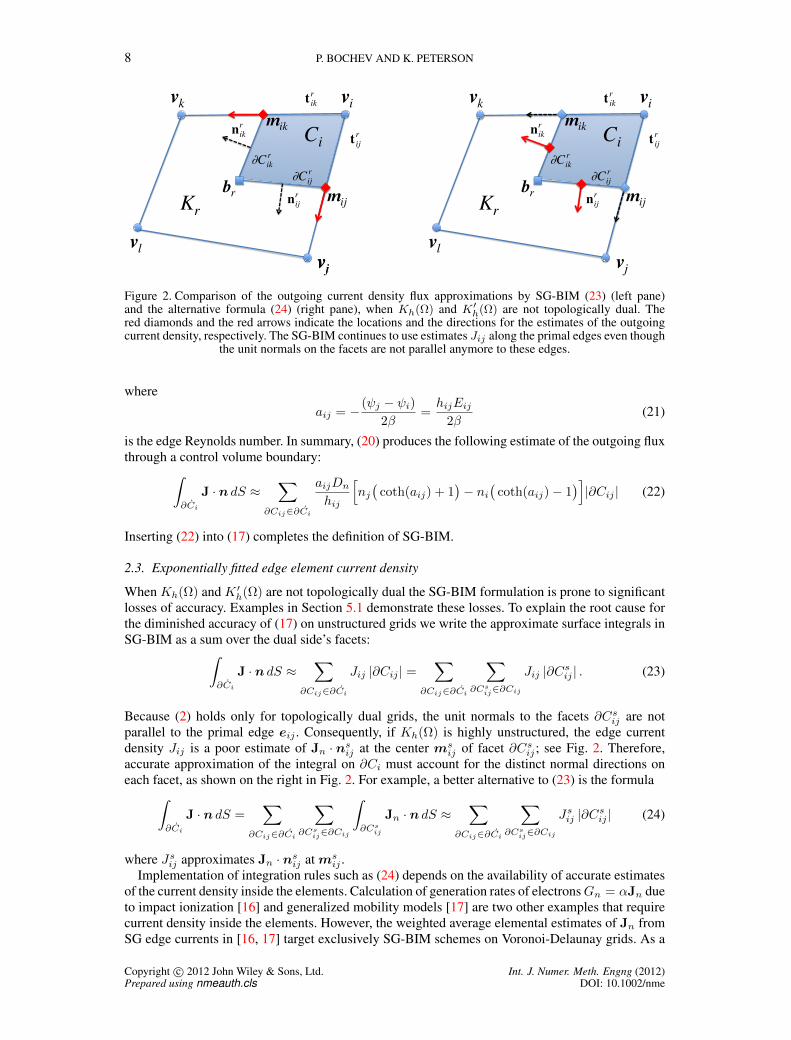
Figure 2. Comparison of the outgoing current density flux approximations by SG-BIM (23) (left pane)and the alternative formula (24) (right pane), when Kh(Ω) and K′h(Ω) are not topologically dual. Thered diamonds and the red arrows indicate the locations and the directions for the estimates of the outgoingcurrent density, respectively. The SG-BIM continues to use estimates Jij along the primal edges even though

the unit normals on the facets are not parallel anymore to these edges.

whereaij = − (ψj − ψi)

2β=hijEij

2β(21)

is the edge Reynolds number. In summary, (20) produces the following estimate of the outgoing fluxthrough a control volume boundary:∫

∂Ci

J · n dS ≈∑

∂Cij∈∂Ci

aijDn

hij

[nj(


(coth(aij)− 1

)]|∂Cij | (22)

Inserting (22) into (17) completes the definition of SG-BIM.

2.3. Exponentially fitted edge element current density

When Kh(Ω) and K ′h(Ω) are not topologically dual the SG-BIM formulation is prone to significantlosses of accuracy. Examples in Section 5.1 demonstrate these losses. To explain the root cause forthe diminished accuracy of (17) on unstructured grids we write the approximate surface integrals inSG-BIM as a sum over the dual side’s facets:∫

∂Ci

J · n dS ≈∑

∂Cij∈∂Ci

Jij |∂Cij | =∑

∂Cij∈∂Ci

∑∂Cs

ij∈∂Cij

Jij |∂Csij | . (23)

Because (2) holds only for topologically dual grids, the unit normals to the facets ∂Csij are notparallel to the primal edge eij . Consequently, if Kh(Ω) is highly unstructured, the edge currentdensity Jij is a poor estimate of Jn · nsij at the center ms

ij of facet ∂Csij ; see Fig. 2. Therefore,accurate approximation of the integral on ∂Ci must account for the distinct normal directions oneach facet, as shown on the right in Fig. 2. For example, a better alternative to (23) is the formula∫

∂Ci

J · n dS =∑

∂Cij∈∂Ci

∑∂Cs

ij∈∂Cij

∫∂Cs

ij

Jn · n dS ≈∑

∂Cij∈∂Ci

∑∂Cs

ij∈∂Cij

Jsij |∂Csij | (24)

where Jsij approximates Jn · nsij at msij .

Implementation of integration rules such as (24) depends on the availability of accurate estimatesof the current density inside the elements. Calculation of generation rates of electronsGn = αJn dueto impact ionization [16] and generalized mobility models [17] are two other examples that requirecurrent density inside the elements. However, the weighted average elemental estimates of Jn fromSG edge currents in [16, 17] target exclusively SG-BIM schemes on Voronoi-Delaunay grids. As a



result, consistent extension of these estimates to general unstructured grids may be problematic andhas not been considered.

Our approach relies on H(curl)-conforming (edge) finite elements to expand edge currents (20)into an exponentially fitted elemental current density JE ∈ Ch

D(Ω). Because edge element shapefunctions are available for a wide range of cell shapes, including polygons [11], this strategyis applicable to an equally wide range of unstructured grids Kh(Ω) without requiring that theassociated control volume grid K ′h(Ω) is topologically dual.

To motivate the use of edge elements we examine the base CVFEM (13) in the absence of carrierdrift and establish a relationship between the nodal current Jn(nh) and the edge currents (20).

Theorem 1Assume that carrier drift velocity µnE = 0. Then

Jn(nh) =∑

eij∈E(Ω)

Dn(nj − ni) ~Wij . (25)

Proof. When µnE = 0 the nodal current density (14) reduces to

Jn(nh) = Dn∇nh =∑

vi∈V (Ω)

Dnni∇Ni .

On the other hand, the nodal space GhD(Ω) and the edge element space Ch

D(Ω) belong to an exactsequence (finite element DeRham complex) [2] and so, ∇Ni ∈ Ch

D(Ω). Moreover, in the lowest-order case there holds [4]

∇Ni =∑

eij∈E(vi)

σij ~Wij . (26)

Combining these two identities yields the representation

Jn(nh) =∑

vi∈V (Ω)

Dnni

∑eij∈E(vi)

σij ~Wij

.

Without loss of generality we may assume that σij = −1, i.e., that the vertex order on eij is vi → vj .Then, after reordering the terms in the above formula

Jn(nh) =∑

eij∈E(Ω)

Dn(nj − ni) ~Wij . (27)

This concludes the proof. 2

Corollary 1Assume that Dn is constant along the edges. Under the hypothesis of Theorem 1

Jn(nh) =∑

eij∈E(Ω)

hijJ0ij~Wij , (28)

where J0ij is the solution of (18) in the absence of carrier drift.

Proof. In the absence of carrier drift µnEij = 0 and equation (18) reduces todJ0

ij

ds= 0; J0

ij = Dndn(s)

ds

n(0) = ni and n(hij) = nj .

(29)

A straightforward calculation shows that

n(s) = ni + snj − nihij

and J0ij = Dn

nj − nihij

.



Therefore, hijJ0ij = Dn(nj − ni), which completes the proof. 2

The edge current densities J0ij are the Scharfetter-Gummel estimates of Jn in the absence of

carrier drift. Corollary 1 establishes that in the pure diffusion limit the nodal current density is sumof the edge element basis functions times these estimates. This relationship is the departure pointfor the consistent extension of the edge currents (20) into an elemental current density JE ≈ Jn.Specifically, in the general drift-diffusion case we set

JE =∑

eij∈E(Ω)

hijJij ~Wij , (30)

where the SG formula (20) defines the coefficients Jij . The resulting exponentially fitted currentdensity field

JE =∑

eij∈E(Ω)

aijDn

[nj(


(coth(aij)− 1

)]~Wij (31)

belongs to H(curl,Ω) and is defined on any mesh that supports construction of Nedelec edgeelements. To complete the definition of CVFEM-EFC we replace the nodal current density in thebase CVFEM (13) by JE :

∫Ci

∂nh∂t

dV −∫∂Ci

JE · n dS = −∫Ci

R(ψ, nh, p)dV +

∫∂CN

i

f dS ; ∀i ∈ Ω ∪ ΓN . (32)

We conclude this section with a formal proof that JE is a consistent extension of the representation(28), which motivates its definition (30).

Lemma 1Assume that Dn and µn are constant along the edges, E = −∇ψ, the electric potential ψ varieslinearly between the nodes, un = µnE and (30) defines JE . Then

limun→0

JE = Jn(nh) . (33)

Proof. If un → 0 we must have Eij → 0 for all eij and from (21) it follows that aij → 0 as well.It is straightforward to see that

limaij→0

aij coth(aij) = 1 ,

and so, for every eij

limaij→0

Jij = limaij→0

aijDn

hij

[nj(


(coth(aij)− 1

)]=Dn

hij(nj − ni) = J0

ij .

This concludes the proof. 2

Remark 1The representation of JE in (30) is an instance of a general approach for defining elemental currentfields from lower-dimensional estimates. The idea is to seek an H(curl)-conforming approximationof the current density

Jn ≈∑α

Jα ~Wrα , (34)

where ~W rα span an edge element space of order r, and Jα approximate Jn on lower-dimensional

entities α of the element. For the lowest-order Nedelec element ~Wij the sum (34) specializes to

Jn ≈∑

eij∈E(Ω)

Jij ~Wij ,



and the normalization property (5) yields the relation

Jn · tkl∣∣∣mkl

≈∑

eij∈E(Ω)

Jij

(~Wij · tkl

) ∣∣∣mkl

=Jklhkl

.

The latter impliesJkl ≈ hkl (Jn · tkl)

∣∣∣mkl

. (35)

Thus, the lowest-order edge element formula (34) allows us to construct an elemental current densityfrom one-dimensional estimates of Jn · tij at edge midpoints. In particular, setting Jkl = hijJij ,yields the exponentially fitted approximation (30). A forthcoming paper will examine the possibilityto obtain higher-order elemental estimates of Jn from one-dimensional currents by using (34) withhigher-order Nedelec elements.

3. IMPLEMENTATION

The expanded form of the CVFEM-EFC formulation (32) is∑vj∈Ω∪ΓN

∂nj(t)

∂t

∫Ci

Nj dV −∑

ekl∈E(Ω)

Jkl

∫∂Ci

~Wkl · n dS = −∫Ci

R(ψ, nh, p)dV +

∫∂CN

i

f dS .

(36)With an appropriate discretization in time (36) is equivalent to a linear system of algebraic equationsK~n = ~f for the unknown nodal coefficients ~n = njj∈Ω∪ΓN

of the discrete carrier concentration(15). The rows of the global discretization matrix K correspond to control volumes Ci surroundingthe vertices vi associated with unknown nodal values ni.

In this section we explain computation of the contributions from the control volume boundaryintegrals in (36) to the discretization matrix K. Computation of the integrals on Ci isstraightforward. To this end, it is instructive to rewrite (30) in a “vertex” form by collecting allterms that share the same nodal degree of freedom. For a vertex vj these terms correspond to theedges inE(vj), providing the following equivalent representation of the exponentially fitted current:

JE =∑

vj∈Ω∪ΓN

∑ejk∈E(vj)

σjkajkDn

[nj(coth(ajk) + σjk)

]~Wjk . (37)

It is now easy to see that the contribution from the second term in (36) to Kij is

Kij ←∑

ejk∈E(vj)

σjkajkDn


] ∫∂Ci

~Wjk · n dS .

Typically, Kij is assembled from element matrices Krij . The integrals on the facets of ∂Ci

belonging to an element Kr are the contributions from the control volume boundary integral tothe element matrices Kr

ij :

Krij ←

∑ejk∈E(vj)∩E(Kr)

∑∂Cr

im∈∂Ci∩Kr

σjkajkDn


] ∫∂Cr

im

~Wjk · n dS . (38)

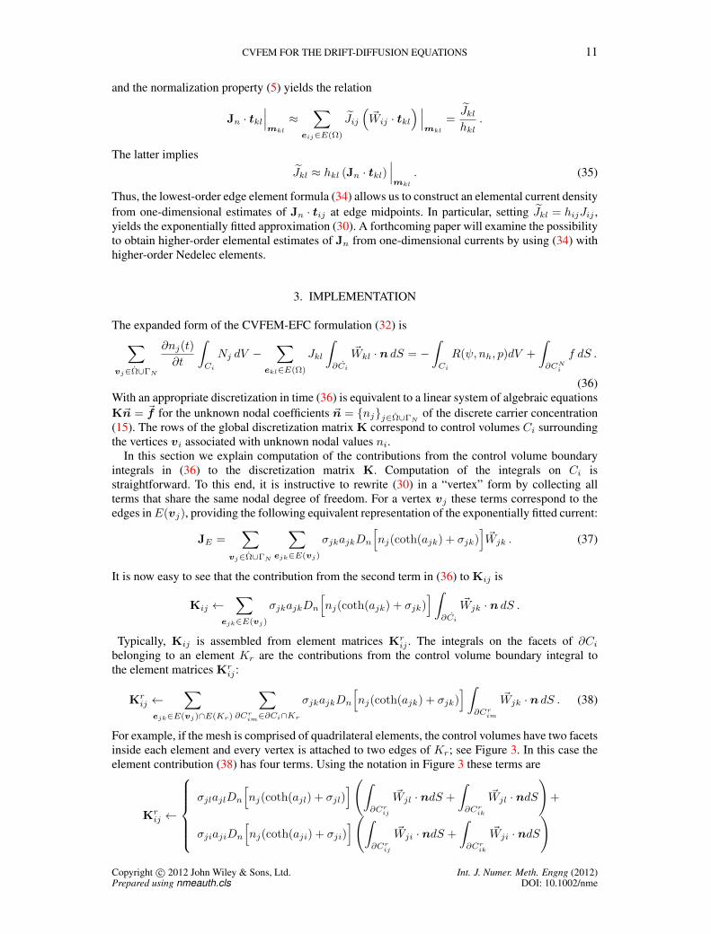
For example, if the mesh is comprised of quadrilateral elements, the control volumes have two facetsinside each element and every vertex is attached to two edges of Kr; see Figure 3. In this case theelement contribution (38) has four terms. Using the notation in Figure 3 these terms are

Krij ←

σjlajlDn

[nj(coth(ajl) + σjl)

](∫∂Cr

ij

~Wjl · ndS +

∫∂Cr

ik

~Wjl · ndS

)+

σjiajiDn

[nj(coth(aji) + σji)

](∫∂Cr

ij

~Wji · ndS +

∫∂Cr

ik

~Wji · ndS

)



Ci!br!

vi!

vj!

mij!

mik!

Kr!

vk!

vl! !

"Cijr

!

"Cikr

!

! W jl

Ci!br!

vi!

vj!

mij!

Kr!

vk!

vl! !

"Cijr

!

"Cikr

!

! W ji

mik!

Figure 3. Assembly of the element contribution (38) to Krij on quadrilateral grids. The control volume Ci

has two facets in Kr: ∂Ci ∩Kr = ∂Crik ∪ ∂Crij (black lines). The vertex vj corresponding to the unknown

nj is attached to two edges: E(vj) ∩ E(Kr) = ejl, eji (red lines). As a result, (38) has four differentterms corresponding to surface integrals of the two basis functions associated with ejl and eji (the red

arrows) on the two control volume facets.

If a nodal coefficient nj corresponds to a vertex on the Dirichlet boundary ΓD, the resulting termscontribute to the right hand side ~f of the linear system. Finally, we note that practical computation ofthe element contributions to K requires suitable cubature rules for the volume and surface integralsin (36).

4. COMPARISON WITH SG-BIM ON CARTESIAN GRIDS

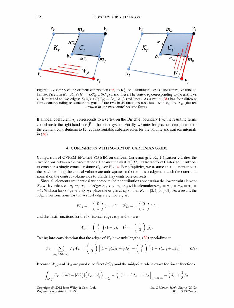
Comparison of CVFEM-EFC and SG-BIM on uniform Cartesian grid Kh(Ω) further clarifies thedistinctions between the two methods. Because the dual K ′h(Ω) is also uniform Cartesian, it sufficesto consider a single control volume Ci; see Fig. 4. For simplicity, we assume that all elements inthe patch defining the control volume are unit squares and orient their edges to match the outer unitnormal on the control volume side to which they contribute currents.

Since all elements are identical we compute their contributions once using the lower right elementKr with vertices vi, vj , vk, vl and edges eij , ejk, elk, eil with orientations σij = σjk = σlk = σil =−1. Without loss of generality we place the origin at vj so that Kr = [0, 1]× [0, 1]. As a result, theedge basis functions for the vertical edges elk and eij are

~Wij = −(

01

)(1− x); ~Wlk = −

(01

)(x);

and the basis functions for the horizontal edges ejk and eil are

~Wjk =

(10

)(1− y); ~Wil =

(10

)(y) .

Taking into consideration that the edges of Kr have unit lengths, (30) specializes to

JE =∑

eij∈E(Kr)

Jij ~Wij =

(10

)[(1− y)Jjk + yJil

]−(

01

)[(1− x)Jij + xJlk

](39)

Because ~Wjk and ~Wil are parallel to facet ∂Crij , and the midpoint rule is exact for linear functions∫∂Cr

ij

JE · ndS = |∂Crij |(JE · nrij

)∣∣∣mr

ij

=1

2

[(1− x)Jij + xJlk

]∣∣∣x=0.25

=3

8Jij +

1

8Jlk



Ci!

vj! vk!

vl!

mij!

Kr!

br!

mil!

!

"Cijr

vi!

!

"Cilr

!

! W jk

!

! W lk

!

! W il

!

! W ij !

milr

!

mijr

Ks!Kt!

Ku!

vn!vm!vr!

vq!

vp!

!

! W mn

!

! W ln

!

! W im

!

! W qr

!

! W qp

!

! W jp

!

! W iq

!

! W mr

1/2! 1/4!

1/2!-3!

1/4!1/2!1/4!

1/2!

1/4! 1!

1!-4!

1!

1!

Figure 4. Notation for a patch of square elements and its control volume. Orientation of edge basis functionsmatches the outer normal direction on the control volume sides. Stencils of CVFEM-EFC and SG-BIM in

the pure diffusion limit.

Likewise, because ~Wij and ~Wlk are parallel to ∂Cril,∫∂Cr

il

JE · ndS = |∂Cril|(JE · nril

)∣∣∣mr

il

=1

2

[(1− y)Jjk + yJil

]∣∣∣y=0.75

=3

8Jil +

1

8Jjk

Combining the facet integrals from all elements results in the approximation∫∂Cij

J · ndS ≈ 1

8Jqp +

3

4Jij +

1

8Jlk and

∫∂Cim

J · ndS ≈ 1

8Jqr +

3

4Jim +

1

8Jln

for the horizontal sides of the control volume, and∫∂Cil

J · ndS ≈ 1

8Jmn +

3

4Jil +

1

8Jjk and

∫∂Ciq

J · ndS ≈ 1

8Jmr +

3

4Jiq +

1

8Jjp

for its vertical sides. In contrast, on the horizontal sides of Ci the SG-BIM approximation of theoutgoing current flux is ∫

∂Cij

J · ndS ≈ Jij and∫∂Cim

J · ndS ≈ Jim

and on the vertical sides this approximation is∫∂Cil

J · ndS ≈ Jil and∫∂Ciq

J · ndS ≈ Jiq .

It is worthwhile to compare these formulas in the pure diffusion limit when Jij = J0ij = Dn(nj −

ni). It is easy to see that in this case the CVFEM-EFC yields the nine-point stencil for the Laplacianon the left in Fig. 4, whereas SG-BIM generates the classical five point stencil shown on the right inthe same figure. In the general case, CVFEM-EFC and SG-BIM correspond to exponentially fittedversions of these stencils.

5. NUMERICAL RESULTS

Section 5.1 examines the accuracy and robustness of the CVEM-EFC using a suite of advection testproblems on uniform and non-uniform grids. Section 5.2 simulates a metal-oxide semiconductorfield-effect transistor (MOSFET) to test the method in a more realistic setting.

5.1. Comparative numerical study

The main objective is to demonstrate that the CVFEM-EFC formulation (32) successfully mergesthe exceptional stability of the classical SG scheme with the generality and the robustness of the



CVFEM. We also want to illustrate and document the severe loss of accuracy in SG-BIM whenKh(Ω) and K ′h(Ω) are not topologically dual. To this end we use a suite of standard test problemsto compare the numerical performance of CVFEM-EFC and SG-BIM on a variety of quadrilateralgrids Kh(Ω). The control volume finite element method with streamline upwinding (CVFEM-SU)[29, 28] provides a benchmark for this comparison. The classical SUPG [8] motivates addition of astreamline diffusion term to the nodal current density

JSU = Jn(nh) + τh(µnE)∇ · ((µnE)nh) , (40)

which defines the CVFEM-SU. The streamline upwind current (40) depends on the stabilizationparameter τh. The paper [29] recommends the value

τh

∣∣∣Ks

=

(cothPes −

1

Pes

)hs

2|µnE|, P es =

|µnE|hs2Dn

; ∀Ks ∈ Kh(Ω) , (41)

which we use in our experiments.

5.1.1. Computational grids In this section Ω is the unit square [0, 1]× [0, 1] with boundary Γ =ΓB ∪ ΓT ∪ ΓL ∪ ΓR, where

ΓB = (x, y) | 0 ≤ x ≤ 1; y = 0; ΓT = (x, y) | 0 ≤ x ≤ 1; y = 1

ΓL = (x, y) | 0 ≤ y ≤ 1;x = 0; ΓR = (x, y) | 0 ≤ y ≤ 1;x = 1 .

The grid Kh(Ω) is logically rectangular but not necessarily uniform partition of Ω into Nx ×Nyquadrilateral elements. Figure 1 shows the construction of the dual grid K ′h(Ω). Coordinate maps

xij = x(ξi, ηj , γ), yij = y(ξi, ηj , γ), 0 ≤ i ≤ Nx, 0 ≤ j ≤ Ny , (42)

where γ is real parameter, and

ξi =i

Nx, i = 0, . . . , Nx; and ηj =

j

Ny, j = 0, . . . , Ny (43)

are the initial uniform grid coordinates, specify the positions of the vertices in Kh(Ω). Our studyuses four different families of grids.

Uniform grids. The coordinate maps x(ξi, ηj , γ) = ξi and y(ξi, ηj , γ) = ηj define a Nx ×Nyuniform grid Kh(Ω). The control volume grid K ′h(Ω) is topologically dual to Kh(Ω).

Randomly perturbed grids. Let rx, ry be uniformly distributed random numbers in [−1, 1]. Thecoordinate maps

x(ξi, ηj , γ) = ξi + 0.25h(rxhγ); y(ξi, ηj , γ) = ηj + 0.25h(ryh

γ) , γ ≥ 0 (44)

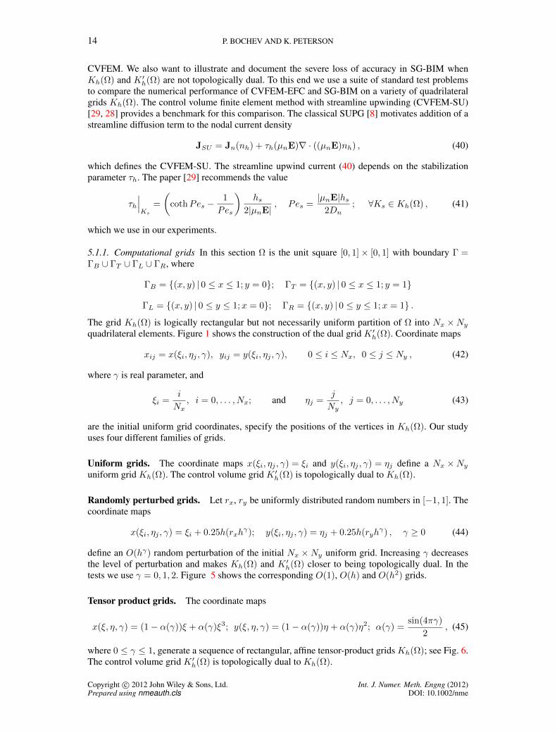
define an O(hγ) random perturbation of the initial Nx ×Ny uniform grid. Increasing γ decreasesthe level of perturbation and makes Kh(Ω) and K ′h(Ω) closer to being topologically dual. In thetests we use γ = 0, 1, 2. Figure 5 shows the corresponding O(1), O(h) and O(h2) grids.

Tensor product grids. The coordinate maps

x(ξ, η, γ) = (1− α(γ))ξ + α(γ)ξ3; y(ξ, η, γ) = (1− α(γ))η + α(γ)η2; α(γ) =sin(4πγ)

2, (45)

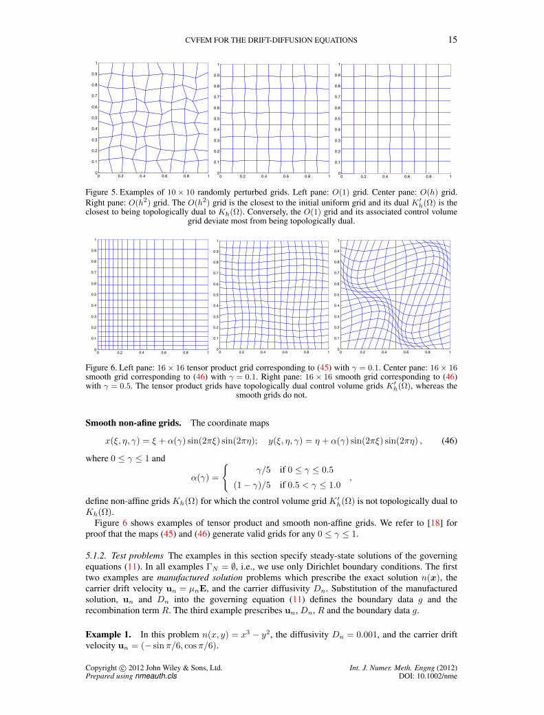
where 0 ≤ γ ≤ 1, generate a sequence of rectangular, affine tensor-product grids Kh(Ω); see Fig. 6.The control volume grid K ′h(Ω) is topologically dual to Kh(Ω).



0 0.2 0.4 0.6 0.8 10

0.1

0.2

0.3

0.4

0.5

0.6

0.7

0.8

0.9

1

0 0.2 0.4 0.6 0.8 10

0.1

0.2

0.3

0.4

0.5

0.6

0.7

0.8

0.9

1

0 0.2 0.4 0.6 0.8 10

0.1

0.2

0.3

0.4

0.5

0.6

0.7

0.8

0.9

1

Figure 5. Examples of 10× 10 randomly perturbed grids. Left pane: O(1) grid. Center pane: O(h) grid.Right pane: O(h2) grid. The O(h2) grid is the closest to the initial uniform grid and its dual K′h(Ω) is theclosest to being topologically dual to Kh(Ω). Conversely, the O(1) grid and its associated control volume

grid deviate most from being topologically dual.

0 0.2 0.4 0.6 0.8 10

0.1

0.2

0.3

0.4

0.5

0.6

0.7

0.8

0.9

1

0 0.2 0.4 0.6 0.8 10

0.1

0.2

0.3

0.4

0.5

0.6

0.7

0.8

0.9

1

0 0.2 0.4 0.6 0.8 10

0.1

0.2

0.3

0.4

0.5

0.6

0.7

0.8

0.9

1

Figure 6. Left pane: 16× 16 tensor product grid corresponding to (45) with γ = 0.1. Center pane: 16× 16smooth grid corresponding to (46) with γ = 0.1. Right pane: 16× 16 smooth grid corresponding to (46)with γ = 0.5. The tensor product grids have topologically dual control volume grids K′h(Ω), whereas the

smooth grids do not.

Smooth non-afine grids. The coordinate maps

x(ξ, η, γ) = ξ + α(γ) sin(2πξ) sin(2πη); y(ξ, η, γ) = η + α(γ) sin(2πξ) sin(2πη) , (46)

where 0 ≤ γ ≤ 1 and

α(γ) =

γ/5 if 0 ≤ γ ≤ 0.5

(1− γ)/5 if 0.5 < γ ≤ 1.0,

define non-affine grids Kh(Ω) for which the control volume grid K ′h(Ω) is not topologically dual toKh(Ω).

Figure 6 shows examples of tensor product and smooth non-affine grids. We refer to [18] forproof that the maps (45) and (46) generate valid grids for any 0 ≤ γ ≤ 1.

5.1.2. Test problems The examples in this section specify steady-state solutions of the governingequations (11). In all examples ΓN = ∅, i.e., we use only Dirichlet boundary conditions. The firsttwo examples are manufactured solution problems which prescribe the exact solution n(x), thecarrier drift velocity un = µnE, and the carrier diffusivity Dn. Substitution of the manufacturedsolution, un and Dn into the governing equation (11) defines the boundary data g and therecombination term R. The third example prescribes un, Dn, R and the boundary data g.

Example 1. In this problem n(x, y) = x3 − y2, the diffusivity Dn = 0.001, and the carrier driftvelocity un = (− sinπ/6, cosπ/6).



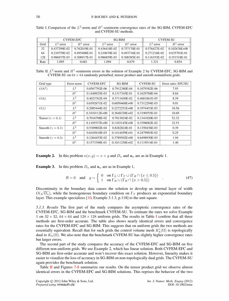
Table I. Comparison of the L2-norm and H1-seminorm convergence rates of the SG-BIM, CVFEM-EFCand CVFEM-SU methods.

CVFEM-EFC SG-BIM CVFEM-SUGrid L2 error H1 error L2 error H1 error L2 error H1 error32 0.437299E-02 0.762019E-01 0.436418E-02 0.757170E-01 0.576427E-02 0.102676E+0064 0.210759E-02 0.495408E-01 0.210670E-02 0.493716E-01 0.271216E-02 0.635701E-01128 0.986937E-03 0.308917E-01 0.986859E-03 0.308385E-01 0.116353E-02 0.351518E-01Rate 1.095 0.681 1.094 0.679 1.221 0.854

Table II. L2-norm and H1-seminorm errors in the solution of Example 2 by CVFEM-EFC, SG-BIM andCVFEM-SU on 64× 64 randomly perturbed, tensor product and smooth nonuniform grids.

Grid type Error norm CVFEM-EFC SG-BIM CVFEM-SU Error ratio: EFC/SU

O(h2) L2 0.8567792E-06 0.7912380E-04 0.1079382E-06 7.93H1 0.1440925E-03 0.1317345E-01 0.1629788E-04 8.84

O(h) L2 0.4023762E-04 0.3711650E-02 0.4681861E-05 8.59H1 0.6592671E-02 0.6050460E+00 0.7312294E-03 9.01

O(1) L2 0.2085444E-02 0.2272251E+00 0.1974453E-03 10.56H1 0.3410112E+00 0.3648320E+02 0.3190555E-01 10.69

Tensor (γ = 0.1) L2 0.7016708E-02 0.7013024E-02 0.1341020E-03 52.32H1 0.1105537E+00 0.1103145E+00 0.3398082E-02 32.53

Smooth (γ = 0.1) L2 0.5309802E-04 0.8282824E-01 0.1350436E-03 0.39H1 0.6165610E-03 0.1414459E+01 0.2479903E-02 0.25

Smooth (γ = 0.5) L2 0.1264453E-02 0.3789502E+00 0.6498930E-03 1.94H1 0.1573398E-01 0.1011258E+02 0.1119514E-01 1.40

Example 2. In this problem n(x, y) = x+ y and Dn and un are as in Example 1.

Example 3. In this problem Dn and un are as in Example 1,

R = 0 and g =

0 on ΓL ∪ ΓT ∪ (ΓB ∩ x ≤ 0.5)1 on ΓR ∪ (ΓB ∩ x > 0.5) . (47)

Discontinuity in the boundary data causes the solution to develop an internal layer of widthO(√Dn), while the homogeneous boundary condition on ΓT produces an exponential boundary

layer. This example specializes [10, Example 3.1.3, p.118] to the unit square.

5.1.3. Results The first part of the study compares the asymptotic convergence rates of theCVFEM-EFC, SG-BIM and the benchmark CVFEM-SU. To estimate the rates we solve Example1 on 32× 32, 64× 64 and 128× 128 uniform grids. The results in Table I confirm that all threemethods are first-order accurate. The table also shows nearly identical errors and convergencerates for the CVFEM-EFC and SG-BIM. This suggests that on uniform grids the two methods areessentially equivalent. Recall that for such grids the control volume mesh K ′h(Ω) is topologicallydual to Kh(Ω). We also note that the benchmark CVFEM-SU has slightly higher convergence ratesbut larger errors.

The second part of the study compares the accuracy of the CVFEM-EFC and SG-BIM on fivedifferent non-uniform grids. We use Example 2, which has linear solution. Both CVFEM-EFC andSG-BIM are first-order accurate and won’t recover this exact solution. However, linearity makes iteasier to visualize the loss of accuracy in SG-BIM on non-topologically dual grids. The CVFEM-SUagain provides the benchmark solution.

Table II and Figures 7-8 summarize our results. On the tensor product grid we observe almostidentical errors in the CVFEM-EFC and SG-BIM solutions. This reprises the behavior of the two



0 0.2 0.4 0.6 0.8 10

0.1

0.2

0.3

0.4

0.5

0.6

0.7

0.8

0.9

1

0 0.2 0.4 0.6 0.8 10

0.1

0.2

0.3

0.4

0.5

0.6

0.7

0.8

0.9

1

0 0.2 0.4 0.6 0.8 10

0.1

0.2

0.3

0.4

0.5

0.6

0.7

0.8

0.9

1

0 0.2 0.4 0.6 0.8 10

0.1

0.2

0.3

0.4

0.5

0.6

0.7

0.8

0.9

1

0 0.2 0.4 0.6 0.8 10

0.1

0.2

0.3

0.4

0.5

0.6

0.7

0.8

0.9

1

0 0.2 0.4 0.6 0.8 10

0.1

0.2

0.3

0.4

0.5

0.6

0.7

0.8

0.9

1

O(h2) O(h) O(1)

Figure 7. Approximation of a globally linear function by CVFEM-EFC (top row) and SG-BIM (bottom row)on 64× 64 randomly perturbed grids. Left: O(h2) grid. Center: O(h) grid. Right: O(1) grid.

methods on uniform grids and is consistent with the fact that, as in the former case, the tensorproduct grid has a topologically dual control volume grid.

The error ratios in Table II verify that on the randomly perturbed grids the accuracy of CVFEM-EFC roughly matches the accuracy of the benchmark CVFEM-SU. On the O(h2) grid, which isclose to a uniform grid, the SG-BIM errors are two orders of magnitude greater but the solution isstill reasonably accurate. However, as the strength of the perturbation increases to O(h) and O(1)the SG-BIM solution deteriorates to a point where the results on the O(1) grid are unusable; seeFig. 7. The severity of the loss of accuracy in SG-BIM correlates with the severity of the loss oftopological duality on the O(h2), O(h) and O(1) grids.

Calculations on smooth non-uniform grids with γ = 0.1 and γ = 0.5 provide an example of amore subtle loss of accuracy in the SG-BIM. As γ increases from 0.1 to 0.5, the loss of topologicalduality between Kh(Ω) and K ′h(Ω) becomes more pronounced and the errors in the SG-BIMsolution grow accordingly; see Fig. 8. Yet, unlike the O(1) random grid case, there are no telltalesigns, such as spurious oscillations, to signal the loss of accuracy. Instead, the degradation of thenumerical solution manifests itself as a smooth mesh imprinting that is hard to detect withoutknowledge of the exact solution. The error ratios in Table II again confirm that the CVFEM-EFCsolution is roughly of the same accuracy as the benchmark CVFEM-SU solution.

The final part of our study demonstrates some advantages stemming from the absence of tunablestabilization parameters in the CVFEM-EFC. The constant advection test problem (47) provides anappropriate setting for this task because it has both an internal and a boundary layer. The middleplots in Fig. 9 show that the CVFEM-SU with the stabilization parameter (41) has significantovershoots across both layers. However, simply increasing the strength of the stabilization term turnsout to be detrimental to the accuracy of the CVFEM-SU. The right plots in Fig. 9 correspond to (41)scaled by a factor of 5 and confirm this. The extra diffusion does not fully eliminate the overshotacross the internal layer, but it smears significantly∗∗ the boundary layer. Clearly, the quality of theCVFEM-SU solution depends critically on the choice of the stabilization parameter. Yet, optimal

∗∗A thorough discussion of this subject, including remedies such as discontinuity capturing, is beyond the scope ofthis paper. We only mention the paper [14], which suggests an alternative definition of the stabilization parameter forelements on the outflow Dirichlet boundary where the boundary layer develops.



0 0.2 0.4 0.6 0.8 10

0.1

0.2

0.3

0.4

0.5

0.6

0.7

0.8

0.9

1

0 0.2 0.4 0.6 0.8 10

0.1

0.2

0.3

0.4

0.5

0.6

0.7

0.8

0.9

1

0 0.2 0.4 0.6 0.8 10

0.1

0.2

0.3

0.4

0.5

0.6

0.7

0.8

0.9

1

0 0.2 0.4 0.6 0.8 10

0.1

0.2

0.3

0.4

0.5

0.6

0.7

0.8

0.9

1

0 0.2 0.4 0.6 0.8 10

0.1

0.2

0.3

0.4

0.5

0.6

0.7

0.8

0.9

1

0 0.2 0.4 0.6 0.8 10

0.1

0.2

0.3

0.4

0.5

0.6

0.7

0.8

0.9

1

tensor grid smooth grid γ = 0.1 smooth grid γ = 0.5

Figure 8. Approximation of a globally linear function by CVFEM-EFC (top row) and SG-BIM (bottom row)on 64× 64 structured nonuniform grids. Left: tensor product grid. Center: smooth grid with γ = 0.1. Right:

smooth grid with γ = 0.5.

0

0.5

1

0

0.5

1

0

0.2

0.4

0.6

0.8

1

0

0.2

0.4

0.6

0.8

1

00.2

0.40.6

0.81

0

0.2

0.4

0.6

0.8

1

1.2

0

0.5

1

0

0.5

1

0

0.1

0.2

0.3

0.4

0.5

0.6

0.7

0.8

0.9

1

0 0.2 0.4 0.6 0.8 10

0.1

0.2

0.3

0.4

0.5

0.6

0.7

0.8

0.9

1

0 0.2 0.4 0.6 0.8 10

0.1

0.2

0.3

0.4

0.5

0.6

0.7

0.8

0.9

1

0 0.2 0.4 0.6 0.8 10

0.1

0.2

0.3

0.4

0.5

0.6

0.7

0.8

0.9

1

Figure 9. Comparison of CVFEM-EFC and CVFEM-SU solutions of the constant advection test problem(47) on 33× 33 O(h) grid. Left: the CVFEM-EFC solution. Center: the CVFEM-SU with (41). Right:

CVFEM-SU with (41) scaled by 5.

selection of this parameter remains an open problem and can be different for different PDEs. Incontrast, the CVFEM-EFC formulation automatically adjusts to the solution features and performsrobustly without any additional calibration and/or adaptation to the problem being solved.



5.2. MOSFET example

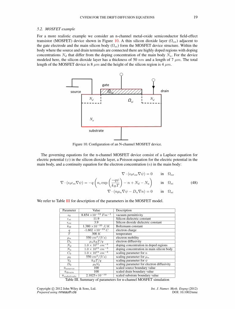
For a more realistic example we consider an n-channel metal-oxide semiconductor field-effecttransistor (MOSFET) device shown in Figure 10. A thin silicon dioxide layer (Ωox) adjacent tothe gate electrode and the main silicon body (Ωsi) form the MOSFET device structure. Within thebody where the source and drain terminals are connected there are highly doped regions with dopingconcentrations Nd that differ from the doping concentration of the main body Na. For the devicemodeled here, the silicon dioxide layer has a thickness of 50 nm and a length of 7 µm. The totallength of the MOSFET device is 8 µm and the height of the silicon region is 4 µm.

!"#$%&' ($)*+',)-&'

!#.!-$)-&'

'Nd 'Nd

'Na

'!ox

'!si

Figure 10. Configuration of an N-channel MOSFET device.

The governing equations for the n-channel MOSFET device consist of a Laplace equation forelectric potential (ψ) in the silicon dioxide layer, a Poisson equation for the electric potential in themain body, and a continuity equation for the electron concentration (n) in the main body:

∇ · (ε0εox∇ψ) = 0 in Ωox

∇ · (ε0εsi∇ψ) = −q(ni exp

(−qψkBT

)− n+Nd −Na

)in Ωsi

∇ · (nµn∇ψ −Dn∇n) = 0 in Ωsi

(48)

We refer to Table III for description of the parameters in the MOSFET model.

Parameter Value Descriptionε0 8.854 ×10−12 Fm−1 vacuum permittivityεsi 11.9 Silicon dielectric constantεox 3.9 Silicon dioxide dielectric constantkB 1.380 ×10−23 J/K Boltzmann constantq -1.602 ×10−19 C electron chargeT 300 K temperatureµn 550 cm2/(V s) electron mobilityDn µnkBT/q electron diffusivityNd 1.0× 1017 cm−3 doping concentration in doped regionsNa 1.0× 1015 cm−3 doping concentration in main silicon bodyC0 1.0× 1015 cm−3 scaling parameter for nµ0 550 cm2/(V s) scaling parameter for µnV0 kBT/q scaling parameter for ψD0 µ0V0 scaling parameter for electron diffusivity

nsource 100 scaled source boundary valuendrain 100 scaled drain boundary value

nsubstrate 2.1025×10−10 scaled substrate boundary valueTable III. Summary of parameters for n-channel MOSFET simulation



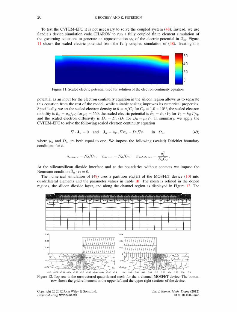
To test the CVFEM-EFC it is not necessary to solve the coupled system (48). Instead, we useSandia’s device simulation code CHARON to run a fully coupled finite element simulation ofthe governing equations to generate an approximation ψh of the electric potential in Ωsi. Figure11 shows the scaled electric potential from the fully coupled simulation of (48). Treating this

Figure 11. Scaled electric potential used for solution of the electron continuity equation.

potential as an input for the electron continuity equation in the silicon region allows us to separatethis equation from the rest of the model, while suitable scaling improves its numerical properties.Specifically, we set the scaled electron density to n = n/C0 for C0 = 1.0× 1015, the scaled electronmobility is µn = µn/µ0 for µ0 = 550, the scaled electric potential is ψh = ψh/V0 for V0 = kBT/q,and the scaled electron diffusivity is Dn = Dn/D0 for D0 = µ0V0. In summary, we apply theCVFEM-EFC to solve the following scaled electron continuity equation

∇ · Jn = 0 and Jn = nµn∇ψh − Dn∇n in Ωsi. (49)

where µn and Dn are both equal to one. We impose the following (scaled) Dirichlet boundaryconditions for n

nsource = Nd/C0 ; ndrain = Nd/C0 ; nsubstrate =n2i

NaC0.

At the silicon/silicon dioxide interface and at the boundaries without contacts we impose theNeumann condition Jn · n = 0.

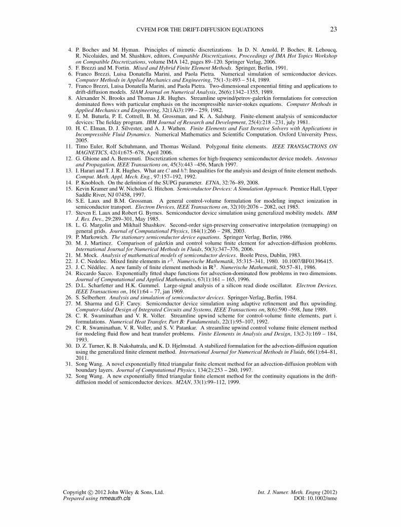
The numerical simulation of (49) uses a partition Kh(Ω) of the MOSFET device (10) intoquadrilateral elements and the parameter values in Table III. The mesh is refined in the dopedregions, the silicon dioxide layer, and along the channel region as displayed in Figure 12. The

−3.6 −3.58 −3.56 −3.54 −3.52 −3.5 −3.48 −3.46 −3.44 −3.42 −3.4

−0.04

−0.02

0

0.02

0.04

0.06

3.4 3.42 3.44 3.46 3.48 3.5 3.52 3.54 3.56 3.58 3.6

−0.04

−0.02

0

0.02

0.04

0.06

Figure 12. Top row is the unstructured quadrilateral mesh for the n-channel MOSFET device. The bottomrow shows the grid refinement in the upper left and the upper right sections of the device.



resulting grid is both highly non-uniform and logically non-rectangular, i.e., E(vi) does not equal 4in all cases. In particular, Figure 12 shows that in the refined regions E(vi) varies between 3 and 6.This represents an additional challenge for methods which rely on topological duality of the controlvolumes.

To demonstrate this challenge we first solve (49) for the manufactured solution in Example 1.Figure 13 shows that the CVFEM-EFC solution correctly represents the linear function despite thehighly unstructured nature of the grid in the upper left and right regions. In contrast, the SG-BIMsolution shows significant numerical errors. The strength of these errors correlates with the regionswhere the grid deviates the most from a logically rectangular topology, i.e., where E(vi) 6= 4.

Test case: linear solution with constant advection, D = 0.01

Upper left corner detail of linear test case.All figures plotted with same color scale.

Exact Solution CVFEM-EFC Results SG-BIM Results







Exact CVFEM-SG SG-BIM

Figure 13. Approximation of a globally linear function on the MOSFET grid. The plots show the exactsolution, the CVFEM-EFC solution and the SG-BIM solution in the upper left portion of the device.

Then we proceed to solve (49) using the approximate electric potential ψh in Figure 11 fromthe fully coupled CHARON solution. Figure 14 shows the scaled electron density for the wholedomain resulting from the CVFEM-EFC simulation. The density is highest along the channel that

Figure 14. Scaled electron density for the n-channel MOSFET computed with the CVFEM-EFC shown overthe full device.

forms below the silicon dioxide layer and between the two doped regions. Figure 15 provides a moredetailed view of the structure of electron density near the source and drain doping regions.

These results agree qualitatively with the fully coupled CHARON solution. They alsodemonstrate that CVFEM-EFC solution remains stable and is not affected adversely by the lackof a logically rectangular grid structure or the large variations in element sizes in the grid.

6. CONCLUSIONS

We presented a new control volume finite element method for the drift-diffusion equations(CVFEM-EFC). The new method combines the exceptional stability of the classical Scharfetter-Gummel upwinding with the generality of CVFEM. On topologically dual grids the CVFEM-EFCis essentially equivalent to the Scharfetter-Gummel Box Integration Method (SG-BIM). However,computational studies in this paper conclusively demonstrate that topological duality of Kh(Ω) andK ′h(Ω) is not necessary for the stability and accuracy of the CVFEM-EFC formulation. The new



Figure 15. Scaled electron density for the n-channel MOSFET computed with the CVFEM-EFC shown overa small section near the source doping region (left) and the drain doping region (right).

method performs robustly on all grids in the studies. Furthermore, the method adapts automaticallyto different types of solution features and does not require heuristic stabilization parameters.

On the other hand, our study confirms that topological duality is a prerequisite for stable andaccurate SG-BIM solution. Without this property (23) fails to provide accurate approximation of thecontrol volume surface integrals. Moreover, violation of topological duality by the control volumemesh K ′h(Ω) not only reduces the accuracy but may lead to unphysical solutions and spuriousoscillations.

ACKNOWLEDGMENT

The authors acknowledge funding by the DOE’s Office of Science Advanced Scientific ComputingResearch Program (ASCR). The Advanced Simulation & Computing (ASC) program of theNational Nuclear Security Administration (NNSA) supported implementation and testing of theCVFEM-EFC.

Conversations with our colleagues G. Hennigan, L. Musson and T. Smith greatly improved ourunderstanding of device modeling and simulation. J. Aidun lent his support and encouraged us tocomplete this work despite the many challenges. We owe special thanks to Xujiao Gao for her helpwith CHARON and especially for generating the electric potentials for the MOSFET simulations inthis paper.

REFERENCES

1. Lutz Angermann and Song Wang. Three-dimensional exponentially fitted conforming tetrahedral finite elementsfor the semiconductor continuity equations. Applied Numerical Mathematics, 46(1):19 – 43, 2003.

2. D. N. Arnold, R. S. Falk, and R. Winther. Finite element exterior calculus, homological techniques, andapplications. Acta Numerica, 15:1–155, 2006.

3. B.R. Baliga and S.V Patankar. New finite element formulation for convection-diffusion problems. Numerical HeatTransfer, 3(4):393–409, October 1980.



4. P. Bochev and M. Hyman. Principles of mimetic discretizations. In D. N. Arnold, P. Bochev, R. Lehoucq,R. Nicolaides, and M. Shashkov, editors, Compatible Discretizations, Proceedings of IMA Hot Topics Workshopon Compatible Discretizations, volume IMA 142, pages 89–120. Springer Verlag, 2006.

5. F. Brezzi and M. Fortin. Mixed and Hybrid Finite Element Methods. Springer, Berlin, 1991.6. Franco Brezzi, Luisa Donatella Marini, and Paola Pietra. Numerical simulation of semiconductor devices.

Computer Methods in Applied Mechanics and Engineering, 75(1-3):493 – 514, 1989.7. Franco Brezzi, Luisa Donatella Marini, and Paola Pietra. Two-dimensional exponential fitting and applications to

drift-diffusion models. SIAM Journal on Numerical Analysis, 26(6):1342–1355, 1989.8. Alexander N. Brooks and Thomas J.R. Hughes. Streamline upwind/petrov-galerkin formulations for convection

dominated flows with particular emphasis on the incompressible navier-stokes equations. Computer Methods inApplied Mechanics and Engineering, 32(1Aı3):199 – 259, 1982.

9. E. M. Buturla, P. E. Cottrell, B. M. Grossman, and K. A. Salsburg. Finite-element analysis of semiconductordevices: The fielday program. IBM Journal of Research and Development, 25(4):218 –231, july 1981.

10. H. C. Elman, D. J. Silvester, and A. J. Wathen. Finite Elements and Fast Iterative Solvers with Applications inIncompressible Fluid Dynamics. Numerical Mathematics and Scientific Computation. Oxford University Press,2005.

11. Timo Euler, Rolf Schuhmann, and Thomas Weiland. Polygonal finite elements. IEEE TRANSACTIONS ONMAGNETICS, 42(4):675–678, April 2006.

12. G. Ghione and A. Benvenuti. Discretization schemes for high-frequency semiconductor device models. Antennasand Propagation, IEEE Transactions on, 45(3):443 –456, March 1997.

13. I. Harari and T. J. R. Hughes. What areC and h?: Inequalities for the analysis and design of finite element methods.Comput. Meth. Appl. Mech. Eng., 97:157–192, 1992.

14. P. Knobloch. On the definition of the SUPG parameter. ETNA, 32:76–89, 2008.15. Kevin Kramer and W. Nicholas G. Hitchon. Semiconductor Devices: A Simulation Approach. Prentice Hall, Upper

Saddle River, NJ 07458, 1997.16. S.E. Laux and B.M. Grossman. A general control-volume formulation for modeling impact ionization in

semiconductor transport. Electron Devices, IEEE Transactions on, 32(10):2076 – 2082, oct 1985.17. Steven E. Laux and Robert G. Byrnes. Semiconductor device simulation using generalized mobility models. IBM

J. Res. Dev., 29:289–301, May 1985.18. L. G. Margolin and Mikhail Shashkov. Second-order sign-preserving conservative interpolation (remapping) on

general grids. Journal of Computational Physics, 184(1):266 – 298, 2003.19. P. Markowich. The stationary semiconductor device equations. Springer Verlag, Berlin, 1986.20. M. J. Martinez. Comparison of galerkin and control volume finite element for advection-diffusion problems.

International Journal for Numerical Methods in Fluids, 50(3):347–376, 2006.21. M. Mock. Analysis of mathematical models of semiconductor devices. Boole Press, Dublin, 1983.22. J. C. Nedelec. Mixed finite elements in r3. Numerische Mathematik, 35:315–341, 1980. 10.1007/BF01396415.23. J. C. Nedelec. A new family of finite element methods in R3. Numerische Mathematik, 50:57–81, 1986.24. Riccardo Sacco. Exponentially fitted shape functions for advection-dominated flow problems in two dimensions.

Journal of Computational and Applied Mathematics, 67(1):161 – 165, 1996.25. D.L. Scharfetter and H.K. Gummel. Large-signal analysis of a silicon read diode oscillator. Electron Devices,

IEEE Transactions on, 16(1):64 – 77, jan 1969.26. S. Selberherr. Analysis and simulation of semiconductor devices. Springer-Verlag, Berlin, 1984.27. M. Sharma and G.F. Carey. Semiconductor device simulation using adaptive refinement and flux upwinding.

Computer-Aided Design of Integrated Circuits and Systems, IEEE Transactions on, 8(6):590 –598, June 1989.28. C. R. Swaminathan and V. R. Voller. Streamline upwind scheme for control-volume finite elements, part i.

formulations. Numerical Heat Transfer, Part B: Fundamentals, 22(1):95–107, 1992.29. C. R. Swaminathan, V. R. Voller, and S. V. Patankar. A streamline upwind control volume finite element method

for modeling fluid flow and heat transfer problems. Finite Elements in Analysis and Design, 13(2-3):169 – 184,1993.

30. D. Z. Turner, K. B. Nakshatrala, and K. D. Hjelmstad. A stabilized formulation for the advection-diffusion equationusing the generalized finite element method. International Journal for Numerical Methods in Fluids, 66(1):64–81,2011.

31. Song Wang. A novel exponentially fitted triangular finite element method for an advection-diffusion problem withboundary layers. Journal of Computational Physics, 134(2):253 – 260, 1997.

32. Song Wang. A new exponentially fitted triangular finite element method for the continuity equations in the drift-diffusion model of semiconductor devices. M2AN, 33(1):99–112, 1999.


a new control volume ﬁnite element method for the stable ... · pdf fileaccurate solution of...

Documents