a new computational approach on signal …

_________________

*Corresponding author

E-mail address: [email protected]

Received December 10, 2020; Accepted January 12, 2021; Published February 19, 2021

1499

Available online at http://scik.org

J. Math. Comput. Sci. 11 (2021), No. 2, 1499-1527

https://doi.org/10.28919/jmcs/5321

ISSN: 1927-5307

A NEW COMPUTATIONAL APPROACH ON SIGNAL PROPAGATION INSIDE

THE COCHLEA

A.N.M. REZAUL KARIM*

Dept. of Computer Science & Engineering, International Islamic University Chittagong, Bangladesh

Copyright © 2021 the author(s). This is an open access article distributed under the Creative Commons Attribution License,which permits

unrestricted use, distribution, and reproduction in any medium, provided the original work is properly cited.

Abstract: Signal propagation inside the cochlea is analyzed from an approximate point of view. This concept has

been established by enabling assumptions regarding the feasibility of modeling experiments on the structure of the

cochlea in line with the expected results of mathematical models. This article sheds light on reviewing the hearing

system from a mathematical, mechanical, electrical, and chemical point of view. This is not to determine which

model is better, but to analyze the advancement of the work on cochlear modeling. This paper attempts to present

which side of the ear and how the Fourier transformation actually performs its function (seperating complex waves

at many frequencies of the sine waves). It provides several improved observations that integrate the effects of the

observed studies in such a way that certain characteristics are captured in different types of liner & non-linear

modeling in Cochlea, which is considered to be a frequency analyzer existing in the inner ear. Our proposed

approach has been developed following advanced computational language-python.

Keywords: Fourier transform; Cochlea; amplitude spectrum; stereocilia (hair cells); basilar membrane (BM); organ

of corti; python (programing language).

2010 AMS Subject Classification: 65T50.

1500

A.N.M. REZAUL KARIM

1. INTRODUCTION

1.1. Anatomy of the Hearing System

Among the sensory organs, it is only the ear that informs us of what is going on in the

surrounding. Therefore, it is an efficient transducer. The brainstem contains various neural

centers. These neural centers also exist in the brain that processes information from the auditory

nerves. Auditory nerves, together with the inner, middle, and outer ear [Figure 1], forms the

peripheral auditory system. Alternatively, the brain and brainstem form parts of the central

nervous hearing organ. The two systems work hand in hand and are responsible for auditory and

hearing perception [1].

Figure 1

1.2. The External Ear

The ear is made up of both a pinna [Figure 1] as well as an external auditory duct. The obtruding

visible part located beside the head is referred to as pinna. It serves an important role in the

hearing process by collecting sound waves from the environment, amplifying the sound, and

funneling it down the canal. The tympanic membrane vibrates if the waves hit the external canal

[2].

` 1501

COMPUTATIONAL APPROACH ON SIGNAL PROPAGATION INSIDE THE COCHLEA

1.3. Middle Ear

Figure 2

It is in this region where the tympanic membrane is located. It is composed of auditory ossicles

(incus, Malleus, and stapes), the Eustachian tube, and lastly, the round and oval window [Figure

2]. The middle ear bones are responsible for sound conduction from the eardrum to interior ear

fluids. The ear in the middle serves the mechanical lever purpose as well as increasing the sound

pressure at the cochlea entrance. The oval window is typically 15 to 30 times lower than that of

the eardrum [3].

Mathematically, pressure increases when the surface area is decreased. Therefore, there is a

decreased area between the two membranes is responsible for the high increase in pressure.

Therefore, it is the imperative to maximize sound quality that comes channeled to the interior ear

fluids. It is also important to regulate pressure inside the ear. For this reason, the ear has got an

Eustachian tube [4] that links the nose and the middle ear . The purpose of the Eustachian tube to

allow equilibrium to be achieved between the middle ear air pressure and that of the atmospheric

air pressure. Equilibrium air pressure is crucial since it allows the eardrum to vibrate freely

efficiently.

1502

A.N.M. REZAUL KARIM

1.4. Inner Ear

Figure 3 Figure 4

The inner part [Figure 3, 4]of the ear comprises of three parts and is enclosed in a temporal bone.

The three parts of the inner ear are the vestibular apparatus, Cochlea, and semicircular canals

(ducts). The Cochlea is a Greek word meaning "snail" due to its spiral shape in appearance.

There are two openings at the base end known as windows. The middle ear is connected to the

oval window while an elastic membrane covers the round window. The Cochlea consists of 3-

coiled canals namely; scala tympani, media (Cochlea duct), and vestibule. An organ is known as

Corti separate scala tympani and media. Corti is built on a flexible basilar membrane.

Additionally, Reissner's membrane is thin and modeled as one chamber, separates the scala

vestibule and scala media [5].

1.5. Functions of Cochlear

Mapping sounds of various frequencies to their respective characteristics positions on the basilar

membrane (BM) is the fundamental function of Cochlea. The fluid-filled Cochlea [Figure 4]

vibrates to respond to oval window motion. The basilar membrane (BM) is moved as it vibrates.

The basilar membrane has varying stiffness and width along its length in a manner that different

parts of the membrane resonate at different frequencies. The thin stiff ends are only moved with

high-frequency vibration while the low frequencies vibrations are responsible for moving the

thick compliant end. The entire transformation can be perceived as an acoustic signal real-time

spectral decomposition procedure that produces spatial frequency in Cochlea. The human ear has

the capability of responding to various frequencies between 20 Hz and 20 KHz as well as various

intensity range up to 120 decibels [6].

` 1503


1.6. The Organ of Corti (Spiral Organ)

Figure 5

This is a tiny organ (organ of Corti) spirally shaped. Corti has got hair cells accountable for

mechanical energy conversion of resulting from basilar membrane vibration into electrical

impulses. The resulting electrical impulses are received by the vestibulocochlear nerve (auditory

vestibular nerve/ auditory nerve), which in turn facilitates the transmission of the information to

the brainstem as well as to the auditory cortex. Corti's organ has around 16,000 audible sensory

hair cells named inner hair cells (IHC) & outer hair cells (OHC), [7] every one having a bundle

of stereocilia (hair bundle), The tips are near to or attached with the tectorial membrane [Figure

5]. The brain stem function is tested several times to see if someone's brain is alive. OHCs are

used to amplify the mechanical signal (i.e. sound) that enter the inner ear, IHCs are the right

receptor cells for hearing and are associated with the nerves [8].

1.7. Cochlea’s Electrical Property

The cochlea’s functions to transform the movement of hair cells into electrical signals. The

motion is the result of incoming sound waves. Once they are converted into electrical signals, the

signals move to the brain through the auditory path neural for processing. Within the Cochlea are

three endolymph and perilymph fluids compartments. The endolymph fluid, contained in the

scala media, is more electrically positive compared to other fluids due to its unique ion content.

The stria vascularis keeps supplying potassium ions [9] into the Cochlea through electromagnetic

pumping to maintain the ionic concentration. The difference in electrical potential creates the

movement of ions through the structures with stable current potentials within the Cochlea.

1504

A.N.M. REZAUL KARIM

As the basilar membrane vibrates, the stereocilia deflect, and the ions flow is modulated. The

stereocilia deflection regulates Mechano-Electrical Transduction channels (MET) [10] opening

and closing. This is largely facilitated by the potential differences that lie between intercellular

potential, perilymph, and endolymph. With the shutting and opening of the MET, the flow of

ions changes, thereby activating the hair cells. It is possible to model the Cochlea into an

electrical model, which is a biological network capacitance, resistance, current, and voltage

sources, by the properties and effects investigation process of the flow of ions, both standing and

alternation.

The Inner hair cells (IHC) transduce mechanical vibrations to stimulate the neural. The neural is

then transmitted to the brain for interpretation, while nonlinear amplification of the BM is the

function of the OHC to make weak stimuli more stable and compress high-level stimuli. It is

reported that the basilar membrane's functioning is associated with both OHC and IHC because

the absence of the OHC lowers the sharpness of tuning and limits the sensitivity to soft sounds.

There is an increase in the dynamic range of hearing associated with the operations of the OHCs.

The electrical lumped model consists of both IHCs and OHCs. Both IHCs and OHCs can be sub-

categorized into basolateral and apical parts [11]. Membrane Voltage, capacitance, resistance

sources can model these subcategories. The Corti organ exhibits similar characteristics to other

biological tissues in the absence of hair cells. In such cases, they can act as a passive electrical

grid. In the presence of hair cells, the sensory epithelium exhibits special electrical properties

that affect its mechanical behaviors. When both electrical and mechanical parts of the Corti

organ interact together, they bring a mutual effect that mediates the cochlea functions. [12]. A

realistic cochlear model should incorporate such interaction.

Figure 6

` 1505


Figure 6 : A diagram representation of the inner as well as OHC. 𝐼 denote the inner hair cells,

and 𝑂 denotes the outer hair cell. MT, 𝑎 and 𝑏 represent the MET channel, basolateral hair cells

parts, and apical [13].

1.8.Chemical Properties of the Hearing System

The three compartments of the Cochlea contain Perilymph and Endolymph fluids [Figure 7].

Within the scala tympani and scala vestibule is the perilymph fluid. The fluid is negatively

charged [14] This has a high sodium content (140mM) and poor calcium content (1,2mM) and

potassium (5mM). The scala media contain endolymph liquid, which is positively charged. This

has a high potassium content (150mM), low in sodium (1mM), and nearly deficient in calcium

(20-30 μM). The lining of the chambers is made up of specialized cells that keep pumping

potassium into the chambers to maintain the concentration difference. Sensory cells use the

chemical energy (like a battery) generated by the difference in the chemical composition of the

fluid to conduct their activities. The membrane of the chambers is made up of tightly-compacted

cells that prevent the fluids from mixing. [15]

Figure 7

Figure 8: Composition of the two cochlear fluids [16]

1506

A.N.M. REZAUL KARIM

2. LITERATURE REVIEW

The Cochlea is a major sensory component in the auditory system. It is impossible to explicitly

visualize cochlear movements. Therefore, Cochlear Modeling is a significant approach to realize

the efficacy of cochlear function. The model of the inner ear as a one-dimensional structure is a

traditional technique [17,18,19,20,21,22].

Cochlea's model occurs in various forms and formulations. These structures are made up of

beams or plates and fluids [23] which constitute electrical properties [24] such as amplifiers,

diodes, capacitors, resistance, and inductors. Mathematical construction and calculation of the

structures are possible. The newly developed finite-element approach employed in several 3-

dimensional concepts [Figure 12 ] in the middle ear [25,26,27,28,29,30,31]. The earlier model of

one-dimension [32,33] held that the fluid pressure of the cochlea channel is constant. Ranke and

Zwislocki also made similar assumptions in their Two-dimensional model. Ranke [34] used the

deep water approximation in his model, while Zwislocki [35] used the shallow water theory.

However, measurement results [36] have found some discrepancies with these assertions. As a

result, Beyer [37] developed a 2-dimensional model of computation which holds that the Cochlea

is flat with rectangular strips. The strips are equally split into 2-sections by a line referred the

basilar membrane [Figure 11].

There are also many cochlea models, such as the Cochlear model of the nonlinear time

domain[13,14,15,16], accompanied by an auditory nerve (AN) response model. An outer hair

cell model [17,18] computed mechanical models [38,39,40,41,42]. and physical models. These

models are made from metal and plastic material or electrical network [43,44,45]. Every slice of

the model in which the Cochlea is split longitudinally into finite segments has about 1 to over

1000 degrees of freedom [46.47]. Before, the cochlea models were meant for simulating the

phase and magnitude of the passive, linear responses into one stimulation tone [48,49.50,51,52].

The subsequent development of the models’ incorporated nonlinearity [53,54,55,56] and active

processes. The nonlinear models used either the perturbation [57,58,59] or iterative techniques to

solve the frequency domain or in the time domain [60,61,62,63,64,65]. The first discovery of the

` 1507


nonlinearity of the Cochlea was made in 1971 by Rhode [66], who reported that higher-level

stimuli have less frequency selectivity in BM's response to sinusoidal stimuli. The advancement

of measurement technologies furthers affirmed that the Cochlear is both functional and

nonlinear.

There is the simulation of neural-like tuning in basilar membrane displacements by the

responsive prototypes of cooblear mechanics. Passive models can simulate postmortem

measurements of the basilar membrane displacements. The prevailing advancement in

computational resources that provide numerical solutions has enhanced the rapid development of

mathematical models of cochlea mechanics.

The processing of signal through the cochlear can be represented by a wavelet transform [67,68].

)i(dt)s

ut(

s

1)t(f)u,s(Wf * −−−−−−−−−−−

−=

−

The wavelet work is designed to find some form of equilibrium between the time domain and the

frequency domain. One can see extremely low-frequency sections everywhere when it is

extended and interpreted the parent wavelet, whereas a high-frequency section can be decisively

located at little s. At the heart of this representation, there are two basic rules: linearity and

scaling. It is understood from their research that the Cochlea conducts a wavelet transformation.

The cochlear channel characterizes the wavelet. The fact that a wavelet transformation is played

out by the Cochlea - in a first guess - seen in the above writing in 1992.

Wavelets refer to the linear transformation process. The wavelets are reliant on parameters and

this method is consistent with the statement of signal processing by wavelet transformations

process in the cochlea.

To date, the investigator has proposed a variety of potential alternatives to seeking a suitable

technique for a successful solution to the hearing system. Here, we proposed a new approach to

the hearing system to achieve a simple, workable solution.

In our newly proposed method, we have also followed these typical methods to present the

cochlear function. However, the main difference of our method with the available literature is

that it has been developed based on the latest computational scheme which makes the

calculations very convenient. Due to the advancement of computational language and associated

1508

A.N.M. REZAUL KARIM

coding, this method provides the desired results immediately following a simple input (with

some basic data). In fact; the proposed method shows very user-friendly and contains a two-step

simple process.

3. THE THEORETICAL CONCEPT OF THE HEARING SYSTEM

Sensory organs such as skin, tongue, ear, and eye are specifically sensitive to certain forms of

energy. For instance, chemical energy is detected by the nose and tongue. On the other hand,

light energy is detected by the eye, while mechanical energy is detected by the skin. The

existence of specialized sensory cells makes it possible for all the sensory organs to convert the

signals from the environment into electrical energy. The electrical energy contains charges and is

converted into numeral code, which is then passed to the brain. The cochlea in the inner ear is a

complex three-dimensional system in which the sensory hair cells [Figure 9] codify sound into

electrical impulses that pass to the brain through the auditory nerve.

Figure 9

The Cochlea is made up of a spiral of tissue filled with fluid in our inner ears and thousands of

tiny hairs [Figure 9] that progressively get smaller from the outside of the spiral to the inside.

Every hair is attached to the nerve. The longer hair resonates at lower frequencies, and the

smaller hair resonates at higher frequencies [Figure 10]. Sounds is complex wave composed of

various signals having distinct amplitudes and frequencies

` 1509


How does sound travel through the ear to the brain:

i. The pinna captures sound waves and directs them down the outer auditory channel,

where the tympanic membrane is struck and vibrated.

ii. Eardrum vibrations force a series of three tiny bones toward each other: the malleus,

the incus, and the stapes, pushing them back and forth.

iii. Inside the cochlea, the movement of the stapes against the cochlea transmits pressure

waves into the fluid, triggering the vibration of the fluid.

iv. The fluid movements trigger tiny hair cells that move softly back and forth inside the

cochlea. As the hair cells move, they release chemical signals that activate nerve

fibers near the cochlea.

v. The signals are sent to the auditory nerve and to the brain by the nerve fibers

Figure 10

3.1. Mathematical Modeling

3.1.1. Linear Model: An auditory signal f(t) in the form of a pressure vacillation causes the

motion u(x, t) of the basilar membrane [Figure 11] in the x-direction in the cochlea. At a

specified level of acoustic pressure, the interaction between the input signal and the activity of

the basilar membrane is remarkably linear. Nevertheless, the process is extremely impressive

with regards to sound intensity, and therefore, it can not be linear. The "quasilinear pattern" is

taken care of in the present environment. It is a model that relies on the factors, e.g. the sound

pressure level in the present scenario. The model is a linear one for set parameters. The values of

these set parameters are represented as a linear expressions of the procedure. An example of a 2-

dimensional frame with a fluid thickness study [69,70]. In this concept, a plane depicts the

outline of the cochlear and the BM by an endless line separating the plane into two sections.

1510

A.N.M. REZAUL KARIM

Figure 11: A 2-dimensional model of the cochlea

3.1.2. Non-linear Modeling

To display the non-linear characteristics of the Cochlea, To understand the context we need to

explain the non-linear function. Usually, the independent variable is u and the dependent variable

is V

V = 𝐻 (𝑢) -------------------(ii)

If any constant factor-like multiplies u then the relation is

𝛽V = 𝐻 (𝛽𝑢) .----------------------------(iii)

For multiple variables of input data 𝑢1, 𝑢2, . . . , 𝑢𝑛, then the relationship is

𝐻 (𝑢1 + 𝑢2 + ⋅ ⋅ ⋅ + 𝑢𝑛) = 𝐻 (𝑢1) + 𝐻 (𝑢2) + ⋅ ⋅ ⋅ + 𝐻 (𝑢𝑛) -------------------------(iv)

The linear method can not produce signal components that are absent in the stimulation range,

nevertheless, every non-linear method can generate Harmonic distorting goods in reaction to

different tonal stimulation. So more complicated stimuli generate more diverse distortion

spectrums of the substance. A time-domain analysis is typically appropriate to analyze cochlear

nonlinear behavior.

In order to continue the time domain study, all applicable machine equations should be placed

through differentiation and integration where applicable.

Typically, the association between pressure differential, p, and acceleration of BM, ..

,at various

locations, x, around the cochlea, may be represented as follows

)x(h

2

x

)x( ..

2

2

−=

---------------- (v)

The behavior of BM relates to the differentiation in pressure as

` 1511


𝑝 (𝑥) = 𝑚 (𝑥) ..

+ 𝑟 (𝑥, 𝑤 ̇) 𝑤 ̇ + 𝑠 (𝑥) 𝑤, --------------- (vi)

where the assumption is that mass is a stable

From the equations (v) & (vi),

[𝑟 (𝑥, 𝑤 ̇) 𝑤 ̇ + 𝑚 (𝑥) ..

+ 𝑠 (𝑥) 𝑤]𝑥𝑥 = 2𝜌/ℎ 𝑤 ̈ (𝑥) , ---------- (vii)

where [ ]𝑥𝑥 means 2nd times derivatives with respect to x.

The differential equations of 2nd order can also be modified as sets of differential equations of

1storder, that can be formulated using method Runge-Kutta.

Figure 12: A 3-dimensional model of the cochlea.

The "shell" is separated into two part and packed with incompressible inviscid liquid (Fig. 11, 12

& 13). The top section is scala vestibule and the lower section is scala tympani, the division is

geometrically symmetrical. Here, L indicates the Box length, W means width and H means

height.

The pressure Dispersion shall differ seamlessly at the canal boundaries

HzWyLx 0;0;0

Say, p denotes the gap between the top portion channel ucp and bottom portion channel lcp in

pressure

)z,y,x(p)z,y,x(p)z,y,x(p uclc −= ---------------------------(viii)

P needs to fulfill Laplace's theorem with relevant boundary limits and the fundamental

calculation may be formulated for cochlear macro mechanics as follows.

0z

p

y

p

x

pp

2

2

2

2

2

22 =

+

+

--------------------------------------(ix) Then p is a harmonic function.

At the border restriction, the fluid passes straight to the neighboring surface with the same flow

effect.

1512

A.N.M. REZAUL KARIM

and the acceleration at a basal wall is )z,y(s

..

)z,y(2)z,y,0(px

s

..

=

-------------------------------(x)

and the apical wall is stationary:

0)z,y,L(px

=

--------------------------------(xi)

Both immobile at the side walls are

0)z,0,x(py

=

---------------------------------(xii)

And

0)z,W,x(py

=

---------------------------------(xiii)

Figure 13

The acceleration in divider border is )y()x(1

..

:

)y()x(2)0,y,x(pz

1

..

=

---------------------------------(xiv)

and the top surface does not shift:

0)H,y,x(pz

=

-------------------------------------(xv)

Usually, a cochlear container layout is a 3-dimensional depiction of the cochlea, As the liquid

has the potential to flow throughout all directions. The cochlear box is considered to be

symmetrical. Above and below the BM are two liquid chambers of the same size [46]. Therefore,

the pressure levels of both chambers are similar and opposite. and it is easier to operate using a

` 1513


single distribution (x , y , z) , similar to the gap in pressure. which doubles the pressure for every

chamber.

4. METHODOLOGY

In the past, when researchers created different methods, programming language and skills did not

improve so much at that time. Recent advances in rapid computing and the development of user-

friendly methods have led to more practical approaches. In this case, the advanced

computational language-Python has been followed in our proposed method and a programming

platform-MATLAB. A necessary mathematical tool used in signal analysis is termed as Fourier

Transform. The sound wave is represented in the time domain as a series of pressure changes

(motions/oscillations) that occur over time.

Figure 14

Fourier Transform changes the domain of the signal, time domain to frequency domain. A

sinusoidal signal in the time-domain is the relating energy (amplitude ) at that particular time.

The spectrum thus represents the respective energy (amplitude) at that specific frequency when a

Fourier transform is introduced. [Figure 14]

We have

)xvi(dte)t(f)(g ti −−−−−−−=

−

−

]f2[ =

)]t(f[F)(g = -----------------(xvii)

)](g[F)t(f 1 = − --------------------------(xviii)

1514

A.N.M. REZAUL KARIM

The equation (xvii) and (xviii) are named a Fourier transform pair; )(g is considered the

Fourier transform of f (t) and conversely, f (t) is regarded as the inverse Fourier transform of

)(g .

From the linear algebra level, the signal may be decomposed into a linear base combination if the

signal is in a base spanned space, it is,

)t(a)t(f kk

k= -----------------------------(xix)

Here, k represents a pointer, ka is the coefficients of )t(k and )t(k are complex functions,

Again, =

−=

k

tjkkec)t(f ---------------- (xx) This is known as the complex form of the Fourier

series.

From (xvii) & (xviii), = )t(ktjk

e

The Real part of the complex function tjke

is tcos , that is, teRtj =

cos)( [

titeti +=

sincos ]

5. PROPOSED METHOD

The stages of the proposed new approach are listed below

Phase 1: The ear receives sound waves which are broken down into its constituent sinusoids with

different frequencies and their corresponding amplitudes, which is mentioned frequency

spectrum (line/amplitude spectrum) of the wave.

Phase 2: the conic shape of the cochlea makes a certain frequency resonate at a certain point

inside the cochlea.

Phase 3: The signal can be synthesized in an inverse Fourier transformation process by adding

its constituent frequencies to the brain.

5.1. Algorithm of the Proposed Approach

Following the aforementioned three phases, an algorithm is developed and presented in Table 1.

Infact, this algorithm forms the key workflow or the computational instruction to execute the

` 1515


calculation. Based on this algorithm, the necessary computational code (program code) has been

developed using the python programming language. The developed computer program or code is

shown in Table 2. With the help of this algorithm, one can easily understand the computer

coding language.

Table 1: Algorithm for matching line spectrum with the Hair cells.

1.

2.

3.

4.

5.

6.

7.

8.

9.

10.

11.

12.

13.

14.

PROGRAM Handshaking with Line spectrums of a complex wave by Haircells (Stereocilia) in Cochlea

INPUT: The equation of 𝑎𝑛

INPUT: The equation of 𝑏𝑛

INPUT: The value of frequency 𝑛𝑤

INPUT: The value 𝑛(No of line spectrum)

FOR i:=1 to 𝑛

CALCULATE: The value of 𝑎𝑖,𝑏𝑖

CALCULATE: The value of amplitude𝑅𝑖 = √𝑎𝑖2 + 𝑏𝑖

2

CALCULATE: The value of frequency i𝑤

DRAW: line spectrum with respect to frequency=i𝑤 and amplitude=𝑅𝑖

ENDFOR

END

15.

16.

17.

18.

19.

20.

21.

22.

23.

24.

25.

26.

27.

28.

29.

30.

PROGRAM match line spectrum with the haircells

FOR i:=1 to 𝑛

SET: Flag:= 0

FOR j:=1 to the all thehaircells

IF line spectrum frequency(i𝑤) equal to haircells_frequency of(j) and line spectrum

amplitude(𝑅𝑖) equal to haircells_height of (j)

THEN line spectrum(i) match to the haircells(j)

PRINT: Haircell(j) receives and Handshakes with Line spectrum(i)

SET: Flag:= 1

ENDIF

ENDFOR

IF Flag equal to 0 (Line spectrum not match with any haircells)

PRINT: Line spectrum(i) not receive by any Haircell

ENDFOR

END

1516

A.N.M. REZAUL KARIM

Table 2: Code for the above algorithm:

import math

import matplotlib.animation as ani

import matplotlib.pyplot as plt

import numpy as np

from mpl_toolkits.mplot3d import Axes3D

def fun_an(an, n):

return eval(an)

def fun_bn(bn, n):

return eval(bn)

def fun_nw(nw, n):

return eval(nw)

input_an = input('Enter an equation in n: ')

input_bn = input('Enter bn equation in n: ')

input_nw = input('Enter nw eqation in n: ')

input_n = input('Enter the value of n: ')

n=eval(input_n)

fig=plt.figure(figsize=(6,5))

ax1=fig.add_subplot(111,projection="3d")

frequency=[]

amplitude=[]

colors=["r","m","g","y","c","orange"]

for i in range(1,n+1):

ai=fun_an(input_an,i)

bi=fun_bn(input_bn, i)

ri=math.sqrt(ai*ai+bi*bi)

amplitude.append(ri)

iw=fun_nw(input_nw, i)

frequency.append(iw)

ax1.bar(frequency,amplitude,zs=1,zdir="y",color=colors,alpha=1)

frequency_hair=[]

height_hair=[]

for i in np.arange(1.0,n+1,0.3):

ai=fun_an(input_an,i)

bi=fun_bn(input_bn, i)

ri=math.sqrt(ai*ai+bi*bi)

height_hair.append(ri)

iw=fun_nw(input_nw, i)

` 1517


6. IMPLEMENTATION

Example 01:

An audio signal 'example_WAV_1MG.wav’ file was read and sampled at 22 kHz. We know the

frequency at which the audio was sampled in order to continue with the analysis. Sounds that we

hear are complex sounds, meaning that they are composed of several frequencies. These

frequencies can be isolated by the cochlea. The simplest way to break down an audio signal into

its frequency components using MATLAB.

MATLAB Code:

>> [y, Fs] = audioread('example_WAV_1MG.wav') % write a matrix of audio data, y, with

sample rate Fs

>> sound(y,Fs) % listen to sound of the above wave.

>> z=length(y)

>> T = length(y)/22000

frequency_hair.append(iw)

ax1.bar(frequency_hair,height_hair,zs=10,zdir="y",color="k",alpha=1)

ax1.set_xlabel('frequency domain (nw)')

ax1.set_zlabel('Amplitude Spectrum ')

plt.show()

def isclose(a,b):

astr=str(a)

aprec=len(astr.split('.')[1]) if '.' in astr else 0

bstr=str(b)

bprec=len(bstr.split('.')[1]) if '.' in bstr else 0

prec=min(aprec,bprec)

return round(a,prec)==round(b,prec)

for i in range(0,n):

flag=0

for j in range(len(frequency_hair)):

if(isclose(frequency[i],frequency_hair[j]) and isclose(amplitude[i],height_hair[j])):

flag=1

print("haircell(",j,") will recieve line spectrum(",i,") and handshake")

if flag==0:

print("any haircell will not recieve line spectrum(",i,")")

1518

A.N.M. REZAUL KARIM

>> f(length(y)+1) = 0

>>t = T*[0:z-1]'/z % Create a vector t the same length as y, that represents elapsed time.

>> plot(t,y)

>>xlabel('Time')

>>ylabel('Audio Signal')

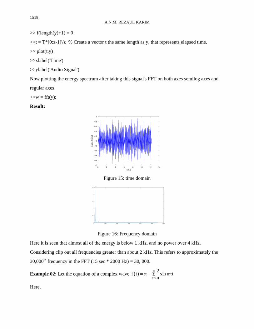
Now plotting the energy spectrum after taking this signal's FFT on both axes semilog axes and

regular axes

>>w = fft(y);

Result:

Figure 15: time domain

Figure 16: Frequency domain

Here it is seen that almost all of the energy is below 1 kHz. and no power over 4 kHz.

Considering clip out all frequencies greater than about 2 kHz. This refers to approximately the

30,000th frequency in the FFT (15 sec * 2000 Hz) = 30, 000.

Example 02: Let the equation of a complex wave

=

−=1n

tnsinn

2)t(f

Here,

` 1519


0=na ; n

2bn = ; = nn

The output of the above complex wave and it’s amplitude spectrum done by MATLAB shown

below:

Result

Figure 17

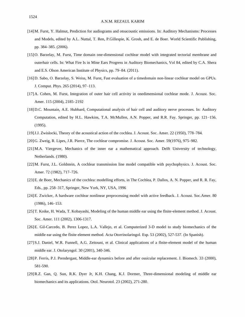
Example 03: The Code for computational approach on signal propagation inside the Cochlea is

shown below using python.

Table 3: Python code for the figure 18

import matplotlib.animation as ani

import matplotlib.pyplot as plt

import numpy as np

%matplotlib inline

from mpl_toolkits.mplot3d import Axes3D

fig=plt.figure(figsize=(5,5))

ax1=fig.add_subplot(111,projection="3d")

#ax1.view_init(30, 30)

#ax1.view_init(25,-135)

ax1.view_init(25,-45)

plt.xlim([3, 19])

plt.xticks(np.arange(3.1416, 19, 3.1416))

colors=["r","m","g","y","c","orange"]

ax1.margins(y=.1, x=.1,z=.1)

def draw_barchart(z_axis):

ax1.clear()

ax1.set_xlim(3.1416, 19)

ax1.set_xticks(np.arange(3.1416, 20, 3.1416))

n=np.arange(start=1, stop=7, step=1)

n1=np.arange(start=1, stop=6.3, step=0.2)

x2=np.multiply(n1,np.pi)

y2=np.divide(2, n1)

x1=np.multiply(n,np.pi)

y1=np.divide(2, n)

plt.subplots_adjust(wspace=0.5, hspace=0.5, left=0.2, bottom=0.2, right=0.9, top=0.9)

ax1.bar(x1,y1,zs=1,zdir="y",alpha=0)

1520

A.N.M. REZAUL KARIM

Result:

Figure 18 [Live: https://bit.ly/3n00Vjm]

For the above figure 18, the following link is shown for Live Signal Propagation within the

Cochlea. https://bit.ly/3n00Vjm

ax1.bar(x1,y1,zs=z_axis,zdir="y",color=colors,alpha=1)

ax1.bar(x1,y1,zs=10,zdir="y",color="royalblue",alpha=1,label='Haircells(Stereocilia)')

ax1.bar(x2,y2,zs=10,zdir="y",color="k",alpha=0.4,label='Haircells(Stereocilia)')

ax1.set_xlabel('frequency domain (nw)')

ax1.set_zlabel('Amplitude Spectrum ')

#ax1.set_zlabel('ZZZZZZZZZZZZ(z)', linespacing=3.4)

plt.tight_layout()

ax1.legend()

plt.box(False)

draw_barchart(1)

plt.show()

import matplotlib.ticker as ticker

import matplotlib.animation as animation

from IPython.display import HTML

animator = animation.FuncAnimation(fig, draw_barchart,frames=range(1,11),interval=500)

animator.save('code.gif', writer='pillow')

HTML(animator.to_jshtml())

https://bit.ly/3n00Vjm


` 1521


7. DISCUSSION

This paper examines current knowledge and reports new findings on some of the nonlinear

processes underlying the mammalian cochlea's work. These processes take place within

mechano-sensory hair cells that form part of the organ of Corti.

In example 1, A complex signal has been taken as a sample. The Matlab code shows the

frequency and amplitude of the sine wave inside this signal. Figure 15 shows the complex wave

in the time domain and figure 16 shows the frequency spectrum of complex wave in the

frequency domain.

In example 2, an equation of a complex signal has been taken as a sample. The Matlab code

presents the frequency and amplitude of the sine wave inside this complex signal. Figure 17

shows the complex wave in the time domain and the corresponding frequency spectrum of

complex wave in the frequency domain.

Figure 18 shows the amplitude of 6 different frequencies in the frequency domain. Here 6

different (as a sample) frequencies are shown with 6 different colors. These are labeled line

spectrum or amplitude spectrum or frequency spectrum. And the hair cells (Stereocilia) of the

cochlea inside the ear are characterized by blue and gray color. When a wave enters the ear then

it is divided into different frequencies. The small hairs in the cochlea resonate with the high

frequency of sine wave and the long hairs in the cochlea resonate with the short frequency of

sine wave. It then travels through the nerves to the brain. How this work is done is shown live in

a link (https://bit.ly/3n00Vjm) made by python language. If the sound or words entered the ear

are not fully heard, the speech is impaired, it is important to understand that a few hair cells are

not working in the cochlea. Then someone needs to take the help of a doctor. How the frequency

spectrum is resonated by the hair-cell is shown three-dimensionally in this paper.

Interestingly, the Cochlea performs the Fourier transform, which is a mathematical tool. In other

words, the inner ear can perform complex calculus and has been doing so way before the

discovery of Fourier transforms in the 19th century. Additionally, the auditory nerve and the hair

cells are responsive to a specific frequency of the sound refers to characteristic frequencies (CF).


1522

A.N.M. REZAUL KARIM

With the entry of force generation, it is possible to tap the CF of hearing nerve and hair cells and

pinpoint their exact location with the aid of a map of tonotopic.

A complex signal f(t) may be viewed as a set of sinusoidal waves. Such sinusoidal forms with

varying types, wavelengths, and voltage levels. The representation of the amplitude, phase, and

frequency of the various signals is referred to as the spectrum of the signal or light. Fourier

Series is a method of evaluating a time-domain signal in order to identify its frequency. In a

nutshell, the time-domain signal is transformed into a frequency-domain through FT.

Conversely, a spectrum may be converted back into a time-domain through the inverse FT.

Sounds consist of a variety of distinct frequencies. Fundamentally, the basilar membrane behaves

like a mechanical FFT computation, and the array of cilia and neurons act as a bank of band-pass

channels. This is the moment when we hear the sound, for example, music and speech, our brain

is getting a bank of action potentials that relate to the FFTs.

8. CONCLUSION

Our proposed method is designed based on a more proper algorithm together with an advanced

computational capability. The existing methods in the literature have been developed long ago

but we developed our method through a new computational approach; hence our method shows

better result. Due to the advancement of computer programming, the proposed method shows

very simple to realize and needs a limited amount of computational time relative to other

approaches available in the literature.

This paper explores the complex properties of the mammalian cochlea and provides some

preliminary findings to demonstrate its unique non-linear components. The modeling has enabled

the understanding of the nature and quantity of knowledge on signal processing and processing

systems in Cochlea. Importantly, it has provided knowledge of the delicate balance between the

phase and amplitude. Basic research is still needed in the hearing system for more accuracy. It is

necessary for cochlear modelers to understand the intended application of models in the clinical

sector.

` 1523


FUNDING

No Funds were received.

CONFLICT OF INTERESTS

The author(s) declare that there is no conflict of interests.

REFERENCE

[1] J. O. Pickles, An Introduction to the Physiology of Hearing, Emerald, Bingley, UK, 2008

[2] R. Patuzzi, Ion flow in cochlear hair cells and the regulation of hearing sensitivity, Hearing Res. 280 (2011), 3–

20.

[3] R. Fettiplace, C. M. Hackney, The sensory and motor roles of auditory hair cells, Nat. Rev. Neurosci. 7 (2006),

19–29.

[4] J. Nam, R. Fettiplace, Force transmission in the organ of corti micromachine, Biophys. J. 98 (2010), 2813–2821.

[5] I.J. Russell, Cochlear receptor potentials, in THE Senses: A Comprehensive Reference, P. Dallos and D. Oertel,

Eds., Elsevier, 2008.

[6] S. L. Johnson, M. Beurg, W. Marcotti, R. Fettiplace, Prestin-driven cochlear amplification is not limited by the

outer hair cell membrane time constant, Neuron, 70 (2011), 1143–1154.

[7] P. Dallos, Some electrical circuit properties of the organ of Corti. I. Analysis without reactive elements, Hearing

Res. 12 (1983), 89–119.

[8] P. Dallos, Some electrical circuit properties of the organ of Corti. II. Analysis including reactive elements,

Hearing Res. 14 (1984) 281–291.

[9] K. H. Iwasa, B. Sul, Effect of the cochlear microphonic on the limiting frequency of the mammalian ear, J.

Acoust. Soc. Amer. 124 (2008), 1607–1612.

[10] E. K. Dimitriadis, R. S. Chadwick, Solution of the inverse problem for a linear cochlear model: a tonotopic

cochlear amplifier, J. Acoust. Soc. Amer. 106 (1999), 1880–1892.

[11] P. Mistrík, C. Mullaley, F. Mammano, J. Ashmore, Threedimensional current flow in a large-scale model of the

cochlea and the mechanism of amplification of sound, J. R. Soc. Interface, 6 (2009), 279–291.

[12] M. A. Cheatham, K. Naik, P. Dallos, Using the cochlear microphonic as a tool to evaluate cochlear function in

mouse models of hearing, J. Assoc. Res. Otolaryngol. 12 (2011), 113–125.

[13] A. Cohen, M. Furst, Integration of outer hair cell activity in onedimensional cochlear mode. J. Acoust. Soc.

Amer. 115 (2004), 2185–2192

1524

A.N.M. REZAUL KARIM

[14] M. Furst, Y. Halmut, Prediction for audiograms and otoacoustic emissions. In: Auditory Mechanisms: Processes

and Models, edited by A.L. Nuttal, T. Ren, P.Gillespie, K. Grosh, and E. de Boer. World Scientific Publishing,

pp. 384–385. (2006).

[15] O. Barzelay, M. Furst, Time domain one-dimensional cochlear model with integrated tectorial membrane and

outerhair cells. In: What Fire Is in Mine Ears Progress in Auditory Biomechanics, Vol 84, edited by C.A. Shera

and E.S. Olson American Institute of Physics, pp. 79–84. (2011).

[16] D. Sabo, O. Barzelay, S. Weiss, M. Furst, Fast evaluation of a timedomain non-linear cochlear model on GPUs.

J. Comput. Phys. 265 (2014), 97–113.

[17] A. Cohen, M. Furst, Integration of outer hair cell activity in onedimensional cochlear mode. J. Acoust. Soc.

Amer. 115 (2004), 2185–2192

[18] D.C. Mountain, A.E. Hubbard, Computational analysis of hair cell and auditory nerve processes. In: Auditory

Computation, edited by H.L. Hawkins, T.A. McMullen, A.N. Popper, and R.R. Fay. Springer, pp. 121–156.

(1995).

[19] J.J. Zwislocki, Theory of the acoustical action of the cochlea. J. Acoust. Soc. Amer. 22 (1950), 778–784.

[20] G. Zweig, R. Lipes, J.R. Pierce, The cochlear compromise. J. Acoust. Soc. Amer. 59(1976), 975–982.

[21] M.A. Viergever, Mechanics of the inner ear a mathematical approach. Delft University of technology,

Netherlands. (1980).

[22] M. Furst, J.L. Goldstein, A cochlear transmission line model compatible with psychophysics. J. Acoust. Soc.

Amer. 72 (1982), 717–726.

[23] E. de Boer, Mechanics of the cochlea: modelling efforts, in The Cochlea, P. Dallos, A. N. Popper, and R. R. Fay,

Eds., pp. 258–317, Springer, New York, NY, USA, 1996

[24] E. Zwicker, A hardware cochlear nonlinear preprocessing model with active feedback. J. Acoust. Soc.Amer. 80

(1986), 146–153.

[25] T. Koike, H. Wada, T. Kobayashi, Modeling of the human middle ear using the flnite-element method. J. Acoust.

Soc. Amer. 111 (2002), 1306-1317.

[26] E. Gil-Carcedo, B. Perez Lopez, L.A. Vallejo, et al. Computerized 3-D model to study biomechanics of the

middle ear using the flnite element method. Acta Otorrinolaringol. Esp. 53 (2002), 527-537. (In Spanish).

[27] S.J. Daniel, W.R. Funnell, A.G. Zeitouni, et al. Clinical applications of a flnite-element model of the human

middle ear. J. Otolaryngol. 30 (2001), 340-346.

[28] P. Ferris, P.J. Prendergast, Middle-ear dynamics before and after ossicular replacement. J. Biomech. 33 (2000),

581-590.

[29] R.Z. Gan, Q. Sun, R.K. Dyer Jr, K.H. Chang, K.J. Dormer, Three-dimensional modeling of middle ear

biomechanics and its applications. Otol. Neurotol. 23 (2002), 271-280.

` 1525


[30] D.J. Kelly, P.J. Prendergast, A.W. Blayney, The efiect of prosthesis design on vibration of the reconstructed

ossicular chain: a comparative flnite element analysis of four prostheses. Otol. Neurotol. 24 (2003), 11-19.

[31] Q. Sun, R.Z. Gan, K.H. Chang, K.J. Dormer, Computer-integrated flnite element modeling of human middle ear.

Biomech. Model Mechanobiol. 1(2002), 109-122.

[32] H. Fletcher, On the dynamics of the cochlea. J. Acoust. Soc. Amer. 23 (1951), 637-645.

[33] L.C. Peterson, B.P. Bogert. A dynamical theory of the cochlea, J. Acoust. Soc. Amer. 22 (1950), 369-381.

[34] Ranke. Theory of operation of the cochlea: a contribution to the hydrodynamics of the cochlea. J. Acoust. Soc.

Amer. 22 (1950), 772-777.

[35] J.J. Zwislocki. Analysis of some auditory characteristics, in: R.R. Buck, R.D. Luce, E. Galanter (Eds.),

Handbook of Mathematical Psychology, Wiley, New York, 1965.

[36] G. Zweig, R. Lipes, J.R. Pierce. The cochlear compromise, J. Acoust. Soc. Amer. 59 (1976), 975-982.

[37] R.P. Beyer A computational model of the cochlea using the immersed boundary method, J. Comput. Phys. 98

(1992), 145-162.

[38] E. de Boer, Mechanics of the cochlea: modelling efforts, in The Cochlea, P. Dallos, A. N. Popper, and R. R. Fay,

Eds., pp. 258–317, Springer, New York, NY, USA, 1996

[39] S. T. Neely, D. O. Kim, A model for active elements in cochlear biomechanics, J. Acoust. Soc. Amer. 79 (1986),

1472–1480.

[40] A.A. Parthasarathi, K. Grosh, A.L. Nuttall, Three-dimensional numerical modeling for global cochlear

dynamics, J. Acoust. Soc. Amer. 107 (2000), 474–485.

[41] S. Ramamoorthy, N.V. Deo, K. Grosh, A mechano-electroacoustical model for the cochlea: response to acoustic

stimuli, J. Acoust. Soc. Amer. 121 (2007), 2758–2773.

[42] S.J. Elliott, E.M. Ku, B. Lineton, A state space model for cochlear mechanics, J. Acoust. Soc. Amer. 122 (2007),

2759–2771.

[43] R.D. White, K. Grosh, Microengineered hydromechanical cochler model, Proc. Nat. Acad. Sci. U.S.A. 102

(2005), 1296–1301.

[44] M.J. Wittbrodt, C.R. Steele, S. Puria, Developing a physical model of the human cochlea using microfabrication

methods, Audiol. Neurotol. 11 (2006), 104–112.

[45] M.J. Wittbrodt, C.R. Steele, S. Puria, Fluid-structure interaction in a physical model of the human cochlea, J.

Acoust. Soc. Amer. 116 (2004), 2542–2543.

[46] C.R. Steele, L.A. Taber, Comparison of WKB calculation and experimental results for three dimensional

cochlear models, J. Acoust. Soc. Amer. 65 (1979), 1007–1018.

1526

A.N.M. REZAUL KARIM

[47] J. Baumgart, C. Chiaradia, M. Fleischer, Y. Yarin, R. Grundmann, A.W. Gummer, Fluid mechanics in the

subtectorial space, in Proceedings of the 10th International Workshop on the Mechanics of Hearing Keele

University, Staffordshire, UK, N. P. Cooper and D. T. Kemp, Eds., pp. 288–293, World Scientific.

[48] J. Zwislocki, Theory of the acoustical action of the cochlea, J. Acoust. Soc. Amer. 22 (1950), 778–784.

[49] G. Zweig, R. Lipes, J.R. Pierce, The cochlear compromise, J. Acoust. Soc. Amer. 59 (1976), 975–982.

[50] C. R. Steele, L. A. Taber, Comparison of WKB and finite difference calculations for a two-dimensional cochlear

model, J. Acoust. Soc. Amer. 65 (1979), 1001–1006.

[51] J. B. Allen, Cochlear micromechanics—a physical model of transduction, J. Acoust. Soc. Amer. 68 (1980),

1660–1670.

[52] E. de Boer, A cylindrical cochlea model: the bridge between two and three dimensions, Hearing Res. 3 (1980),

109–131.

[53] S.T. Neely, D.O. Kim, A model for active elements in cochlear biomechanics, J. Acoust. Soc. Amer. 79 (1986),

1472–1480.

[54] E. de Boer, On active and passive cochlear models—toward a generalized analysis, J. Acoust. Soc. Amer. 73

(1983), 574–576.

[55] F. Mammano, R. Nobili, Biophysics of the cochlea: linear approximation, J. Acoust. Soc. Amer. 93 (1993),

3320–3332.

[56] C.D. Geisler, C. Sang, A cochlear model using feed-forward outer-hair-cell forces, Hearing Res. 86 (1995), 132–

146.

[57] L.J. Kanis, E. de Boer, Self-suppression in a locally active nonlinear model of the cochlea: a quasilinear

approach, J. Acoust. Soc. Amer. 94 (1993), 3199–3206.

[58] R.S. Chadwick, Compression, gain, and nonlinear distortion in an active cochlear model with subpartitions, Proc.

Nat. Acad. Sci. U.S.A. 95 (1998), 14594–14599.

[59] K. Lim, C.R. Steele, A three-dimensional nonlinear active cochlear model analyzed by the WKB-numeric

method, Hearing Res. 170 (2002), 190–205.

[60] S.J. Elliott, E.M. Ku, B. Lineton, A state space model for cochlear mechanics, J. Acoust. Soc. Amer. 122 (2007),

2759–2771.

[61] J.L. Hall, Two tone distortion products in a nonlinear model of the basilar membrane, J. Acoust. Soc. Amer. 56

(1974), 1818–1828.

[62] D.O. Kim, S.T. Neely, C.E. Molnar, J.W. Matthews, An active cochlear model with negative damping in the

partition: comparison with Rhodes ante- and post-mortem observations, in Psychophysical, Physiological, and

Behavioural Studies in Hearing, G. van den Brink and F. A. Bilsen, Eds., pp. 7–14, Delft University Press, Delft,

The Netherlands, 1980.

` 1527


[63] M. Furst, J. L. Goldstein, A cochlear nonlinear transmission-line model compatible with combination tone

psychophysics, J. Acoust. Soc. Amer. 72 (1982), 717–726.

[64] R.J. Diependaal, H. Duifhuis, H.W. Hoogstraten, M.A. Viergever, Numerical methods for solving one-

dimensional cochlear models in the time domain, J. Acoust. Soc. Amer. 82 (1987), 1655–1666.

[65] A. Moleti, N. Paternoster, D. Bertaccini, R. Sisto, F. Sanjust, Otoacoustic emissions in time-domain solutions of

nonlinear non-local cochlear models, J. Acoust. Soc. Amer. 126 (2009), 2425–2436.

[66] W.S. Rhode, Observations of the vibration of the basilar membrane in squirrel monkeys using the Mossbauer

technique, J. Acoust. Soc. Amer. 49 (1971), 1218.

[67] I. Daubechies, Ten lectures on wavelets. SIAM, Philadelphia, 1992.

[68] R.C. Gonzalez , R.E. Woods, Digital Image Processing (2nd Edition). Prentice Hall, January 2002, pp: 364-365.

[69] C.S.Peskin, Partial difierential equations in biology. Courant Inst. Lecture Notes, Courant Inst. of Mathematical

Sciences, NYU, New York, 1975-1976.

[70] X. Yang, K. Wang, S. Shamma, Auditory representation of acoustic signals. IEEE Trans. Inform. Theory. 38

(1992), 824–839.

a new computational approach on signal …

Documents