a new bidirectional deconvolution method that overcomes the

A new bidirectional deconvolution method that

overcomes the minimum phase assumption

Yang Zhang and Jon Claerbout

ABSTRACT

Traditionally blind deconvolution makes the assumption that the reflectivity spikeseries is white. Earlier we dropped that assumption and adopted the assumptionthat the output spike series is sparse under a hyperbolic penalty function. Thisapproach now here allows us to take a step further and drop the assumptionof minimum phase. In this new method (what we called Bidirectional SparseDeconvolution), We solve explicitly for the maximum phase part of the source.Results on both synthetic data and field data show clear improvements.

INTRODUCTION

In the previous report (Zhang and Claerbout, 2010), we introduced the spiking de-convolution problem using the hybrid norm solver (Claerbout, 2009a). Syntheticexamples (Zhang and Claerbout, 2010) showed that given a minimum-phase wavelet,it retrieved the sparse reflectivity model almost perfectly even with a reflection seriesthat is far from white, while conventional L2 deconvolution did a poor job. However,if the assumption of a minimum-phase wavelet was removed, the hybrid norm spikingdeconvolution failed quickly and gave a poor result similar to the conventional L2deconvolution.

In this paper, we still rely on the hybrid norm solver to retrieve the sparse model,but we use a slightly more complex formulation that avoids the minimum-phasewavelet constraint.

We start by realizing that any (mixed-phase) wavelet C(Z) can be decomposedinto a minimum-phase part A(Z) and a maximum-phase part B(1/Z) plus a certaintime shift:

C(Z) = A(Z)B(1/Z)Zk, (1)

where B(Z) is also a minimum-phase wavelet (therefore B(1/Z)Zk is a maximum-phase wavelet) and the exponent k is the order of B(Z). This Zk term makes thewavelet C(Z) causal. In the time domain, (1) can be written as

c = a ∗ br ∗ δ(n− k), (2)

where br stands for the time reverse of series b.

SEP–142

Zhang and Claerbout 2 Hybrid solver deconvolution

Our original spiking deconvolution can find only a minimum-phase wavelet whichhas the same spectrum of real wavelet c. It can be defined as an inverse problem asfollows:

[d]fc = r, (3)

where [d] is the data convolution operator, and fc is the unknown filter. In thisformulation, the filter is the only unknown, the hybrid norm is applied on the residualterm r to enforce the sparseness constraint. In theory, the residual r itself is thereflectivity model. Such a method requires the wavelet in the data to be minimum-phase because only a minimum-phase wavelet has a causal stable inverse.

The following bidirectional deconvolution formulation utilizes a pair of conven-tional deconvolutions, trying to invert components a and b separately:

[(d ∗ f rb )] fa = ra,

[(d ∗ fa)r] fb = rb,

(4)

in which fa and fb are the corresponding filters that corresponds to the inverses ofa and b denoted above, the superscript r means time-reverse. The operator in eachequation is the convolution operator. Again the hybrid norm is applied to ra andrb, and the reflectivity model is simply ra plus a time shift. Notice that this is anon-linear inversion, since the operator itself depends on the unknown fa and fb. Inpractice we have to solve these two inversions alternately and therefore iteratively.

To understand the meaning of (4), let

d = m ∗ c = m ∗ a ∗ br ∗ δ(n− k), (5)

where m is the reflectivity model and the δ term is just a time shift. Assume fa andfb are perfectly known in the operators (which is not true in reality), i.e.

fa ∗ a = δ(n), fb ∗ b = δ(n)

Substituting (5) into (4), since

d ∗ f rb = m ∗ δ(n− k) ∗ a, (6)

(d ∗ fa)r = (m ∗ br ∗ δ(n− k))r = mr ∗ δ(n + k) ∗ b, (7)

we have[(m ∗ δ(n− k)) ∗ a] fa = ra,[(mr ∗ δ(n + k)) ∗ b] fb = rb.

(8)

From (8) it is easier to see what is behind the bidirectional deconvolution formulation(4): It tries to separate the two parts of the wavelet, turning each one into a traditionaldeconvolution problem in which the wavelet (a, b) is always minimum-phase.

As with all non-linear estimation, iteration is required. Convergence is assured ifthe starting solution is close enough. We expect the traditional PEF for a and animpulse function for b to be a pretty good first guess. The following section showsseveral examples (complexity varies from low to high) illustrating the effectivenessand limitations of the method.

SEP–142


DATA EXAMPLES

Inverting a single wavelet

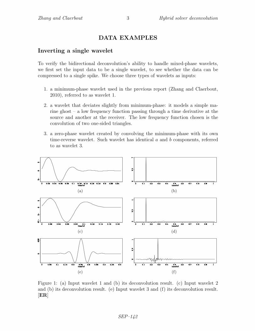
To verify the bidirectional deconvolution’s ability to handle mixed-phase wavelets,we first set the input data to be a single wavelet, to see whether the data can becompressed to a single spike. We choose three types of wavelets as inputs:

1. a minimum-phase wavelet used in the previous report (Zhang and Claerbout,2010), referred to as wavelet 1.

2. a wavelet that deviates slightly from minimum-phase: it models a simple ma-rine ghost – a low frequency function passing through a time derivative at thesource and another at the receiver. The low frequency function chosen is theconvolution of two one-sided triangles.

3. a zero-phase wavelet created by convolving the minimum-phase with its owntime-reverse wavelet. Such wavelet has identical a and b components, referredto as wavelet 3.

(a) (b)

(c) (d)

(e) (f)

Figure 1: (a) Input wavelet 1 and (b) its deconvolution result. (c) Input wavelet 2and (b) its deconvolution result. (e) Input wavelet 3 and (f) its deconvolution result.[ER]

SEP–142


(a) (b)

Figure 2: For the wavelet 3 inversion, (a) filter fa; (b) filter fb. [ER]

Figure 1(a) 1(b), figure 1(c) 1(d) and figure 1(e) 1(f) show wavelets 1,2,3, and theresults of reflectivity models respectively. In all 3 cases, our bidirectional deconvolu-tion method is able to compress the wavelet into a spike.

Figure 2 shows the retrieved filters fa and fb from wavelet 3’s inversion. Noticethat fa and fb given by the inversion are different from each other, while ideally theyshould be the same, since a and b are the same when we create wavelet 3. Thisobservation indicates that the solutions fa and fb of this method do not necessarilyconverge to the inverse of the initial a and b.

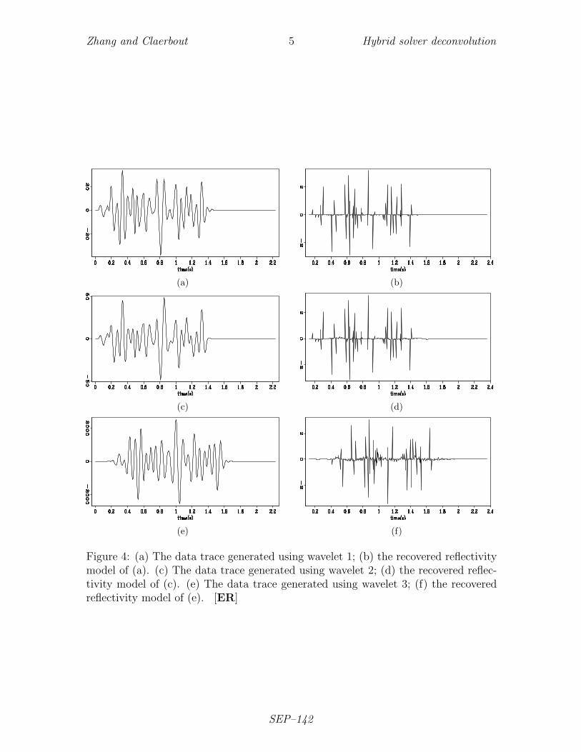
Inverting a synthetic trace

Next we try a more complex example where the data is generated by convolving eachtype of wavelet with a sparse reflectivity series. Figure 3 shows the reflectivity series.

Figure 4(a) 4(b), figure 4(c) 4(d) and figure 4(e) 4(f) show the data created usingwavelets 1,2,3, and the recovered reflectivity models respectively. In all 3 cases, thereflectivity model is well recovered; however the polarity of the reflectivity modelfrom wavelet 3 case is opposite to that of the real reflectivity model; this unexpectedchange of polarity shows the uncertainty of the convergence point in our non-linearformulation. We think this polarity change is not an issue in our blind deconvolutionscenario.

Figure 3: reflectivity model trace. [ER]

SEP–142


(a) (b)

(c) (d)

(e) (f)

Figure 4: (a) The data trace generated using wavelet 1; (b) the recovered reflectivitymodel of (a). (c) The data trace generated using wavelet 2; (d) the recovered reflec-tivity model of (c). (e) The data trace generated using wavelet 3; (f) the recoveredreflectivity model of (e). [ER]

SEP–142


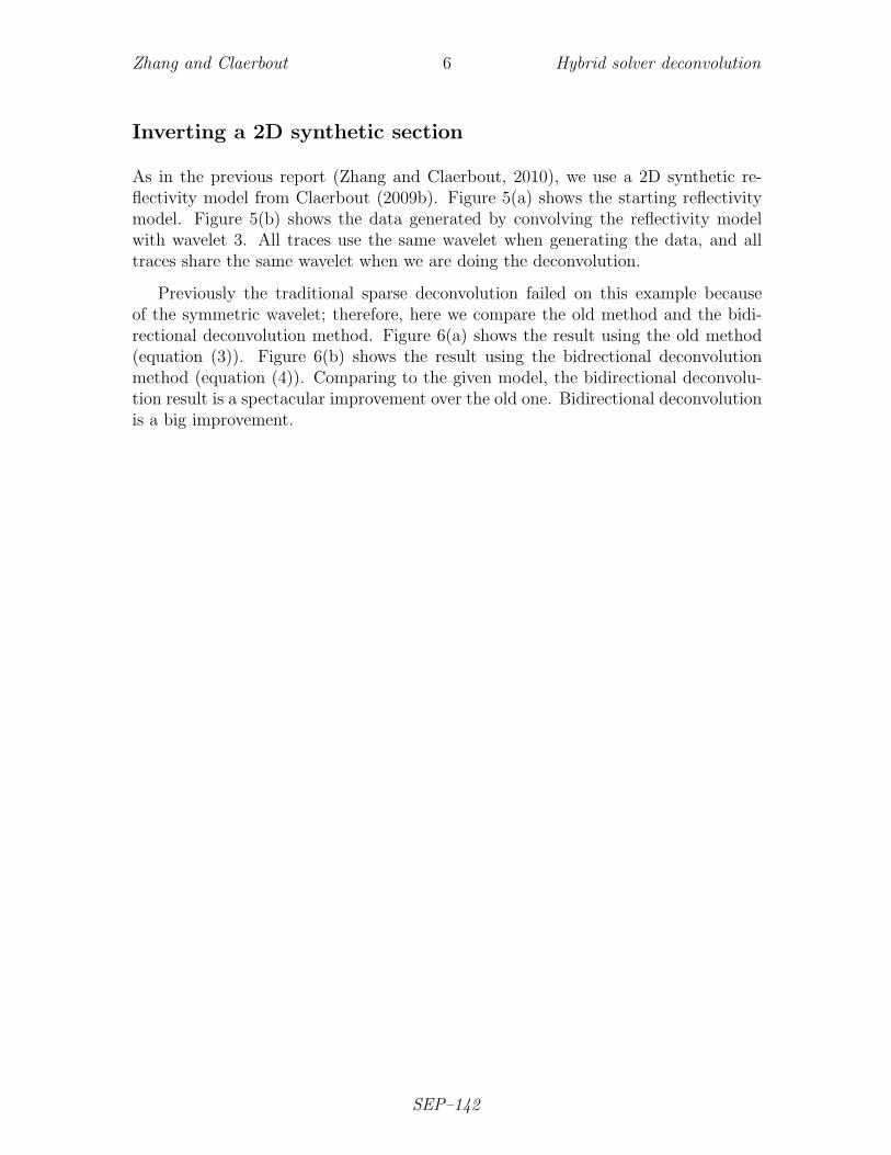
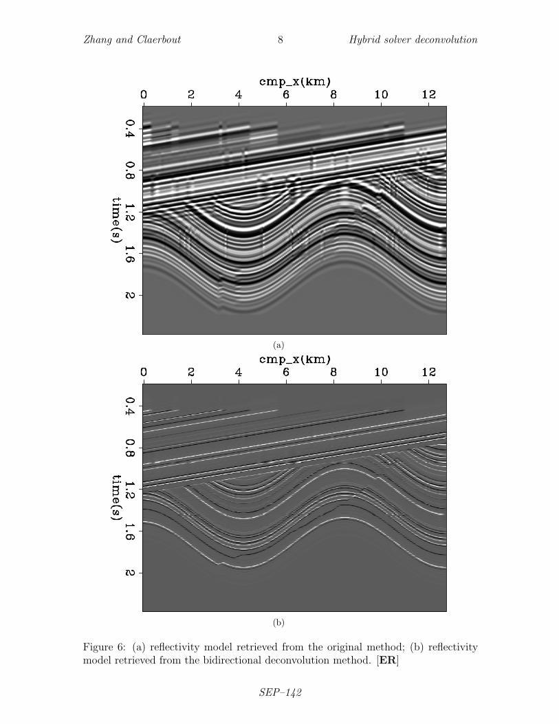
Inverting a 2D synthetic section

As in the previous report (Zhang and Claerbout, 2010), we use a 2D synthetic re-flectivity model from Claerbout (2009b). Figure 5(a) shows the starting reflectivitymodel. Figure 5(b) shows the data generated by convolving the reflectivity modelwith wavelet 3. All traces use the same wavelet when generating the data, and alltraces share the same wavelet when we are doing the deconvolution.

Previously the traditional sparse deconvolution failed on this example becauseof the symmetric wavelet; therefore, here we compare the old method and the bidi-rectional deconvolution method. Figure 6(a) shows the result using the old method(equation (3)). Figure 6(b) shows the result using the bidrectional deconvolutionmethod (equation (4)). Comparing to the given model, the bidirectional deconvolu-tion result is a spectacular improvement over the old one. Bidirectional deconvolutionis a big improvement.

SEP–142


(a)

(b)

Figure 5: (a) The 2D synthetic reflectivity model; (b) the synthetic data generatedusing wavelet 3. [ER]

SEP–142


(a)

(b)

Figure 6: (a) reflectivity model retrieved from the original method; (b) reflectivitymodel retrieved from the bidirectional deconvolution method. [ER]

SEP–142


Inverting a 2D field section

Figure 7: Input Common Offset data. [ER]

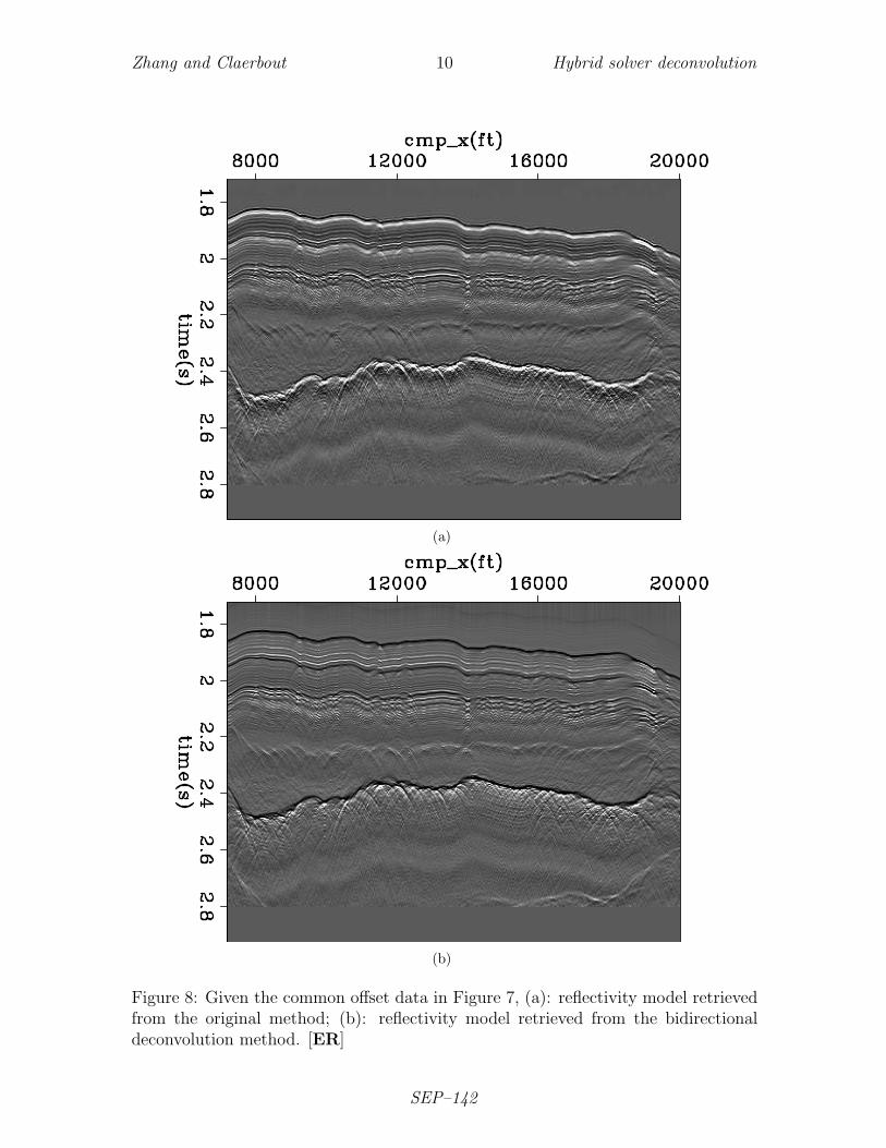
The second example is a common-offset section of marine field data. Figure 7shows the input data. Figure 8(a) shows the result using the old method. Figure 8(b)shows the result using the bidirectional deconvolution method.

The raw data in Figure 7 shows strong events like a double ghost (black, white,black). The traditional PEF result in Figure 8(a) shows strong events like doublets(black, white). The bidirectional deconvolution result in Figure 8(b) shows strongevents like singlets (white). Examining Figure 8(b) we notice events at about 1.85s(black), 1.95s (black), 2.3s (white), 2.4s(black), 2.5s (mixed), and 2.8s (white). Theunipolarity of individual suggests that a causal integration would produce the stepfunctions we associate with impedence in a blocky model. Figure 9 is a first attempt tocompute the impedence from the reflectivity in Figure 8(b). This was done by causalintegration and some horizontal smoothing. Ideally, Figure 8(b) has only isolatedwhite events and black events defining geologic boundaries. Time integrating theseimpulsive events should yield positive rectangle functions. Actually, the result we seein Figure 9 looks more like leaky integration of Figure 8(b). The small events presentin Figure 8(b) apparently contains low frequency energy at the opposite polarity ofthat of the isolated impulses. We could thus regard Figure 9 as a failure. Instead weregard it as an inverse problem that we have not yet correctly posed. The failure arisesbecause the raw data fails to contain the required low frequencies. Were we to replacesmall values in Figure 8(b) by zeros, we might have obtained a result more to ourliking. We need to formalize the inverse problem and reduce it to the usual situation

SEP–142


(a)

(b)

Figure 8: Given the common offset data in Figure 7, (a): reflectivity model retrievedfrom the original method; (b): reflectivity model retrieved from the bidirectionaldeconvolution method. [ER]

SEP–142


Figure 9: Causal time integration of the reflectivity in figure 8(b). This should bethe impedence. [ER]

which is how much to regard the data as perfect, and how to allow imperfection tobe overcome by methodology that tends us to blocky models.

CONCLUSION

We demonstrate what we anticipated theoretically that we can overcome the minimumphase assumption in blind deconvolution. Our process is non-linear, but (we claim)not extremely so. To be successful it does require a non-Gaussian distribution ofimpulses. Likewise, the iteration has a few adjustable parameters which makes itsuse a little more difficult, but we do not anticipate serious difficulties in practice. Oneinteresting phenomenon about the bidirectional deconvolution (Figure 1(e) 1(f) andfigure 2) is that it was able to compress a mixed-phase wavelet to a spike but withoutobtaining the correct causal and anti-causal parts. We do not yet understand this.In addition, it is more costly because it requires multiple iterations.

FUTURE WORK

Having had good fortune here introducing the anti-causal PEF and earlier explicitlyestimating a portion of the data not fitting the convolutional model (Zhang and

SEP–142


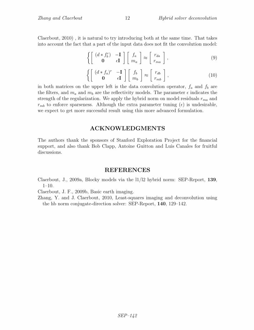
Claerbout, 2010) , it is natural to try introducing both at the same time. That takesinto account the fact that a part of the input data does not fit the convolution model:{[

(d ∗ f rb ) −I

0 εI

] [fa

ma

]≈

[rda

rma

], (9)

{[(d ∗ fa)

r −I0 εI

] [fb

mb

]≈

[rdb

rmb

], (10)

in both matrices on the upper left is the data convolution operator, fa and fb arethe filters, and ma and mb are the reflectivity models. The parameter ε indicates thestrength of the regularization. We apply the hybrid norm on model residuals rma andrmb to enforce sparseness. Although the extra parameter tuning (ε) is undesirable,we expect to get more successful result using this more advanced formulation.

ACKNOWLEDGMENTS

The authors thank the sponsors of Stanford Exploration Project for the financialsupport, and also thank Bob Clapp, Antoine Guitton and Luis Canales for fruitfuldiscussions.

REFERENCES

Claerbout, J., 2009a, Blocky models via the l1/l2 hybrid norm: SEP-Report, 139,1–10.

Claerbout, J. F., 2009b, Basic earth imaging.Zhang, Y. and J. Claerbout, 2010, Least-squares imaging and deconvolution using

the hb norm conjugate-direction solver: SEP-Report, 140, 129–142.

SEP–142


SEP–142

a new bidirectional deconvolution method that overcomes the

Documents