A New Approach to the Valuation of Intangible Capital∗

Jason G. CumminsDivision of Research and Statistics

Board of Governors of the Federal Reserve Systemjason.g.cummins@frb.gov

March 15, 2004

Abstract

Intangible capital is not a distinct factor of production as is physical capital orlabor. Rather it is the “glue” that creates value from other factor inputs. Thisperspective naturally suggests an empirical model in which intangible capital isdefined in terms of adjustment costs. My estimates of these adjustment costsfrom firm-level panel data suggest that no appreciable intangibles are associatedwith R&D and advertising, whereas information technology creates intangibleswith a 72% annual rate of return – a sizable figure that is nevertheless muchsmaller than that reported in previous studies. To build a bridge to previousresearch, I show that much larger estimates can be obtained with ordinary leastsquares, a method that ignores the possibility that the value of the firm and itsinvestment policy are simultaneously determined.

JEL Classification: D24, E22.Keywords: Organizational capital, intellectual property, adjustment costs.

∗Baruch Lev has been instrumental in shaping my thinking about intangible assets. I thank himfor his guidance and for providing me with the dataset on information technology investment that heand Suresh Radhakrishnan put together. I am also indebted to Stephen Bond whose collaborationlaid the foundation for this research. Daniel Cooper provided research assistance. Ned Nadiri,the editors, CRIW conference participants, and Darrel Cohen all provided helpful comments andsuggestions. I/B/E/S International Inc. provided the data on earnings expectations. The viewspresented are solely mine and do not necessarily represent those of the Board of Governors of theFederal Reserve System or its staff members.

1 Introduction

In most circumstances, there are no direct measures of the return on intangible

capital. As a result, researchers have relied primarily on the equity market to infer

the value of intangibles. This valuation method is straightforward: If the equity

market reveals the intrinsic value of the firm, then subtracting the value of the

firm’s tangible assets from its market value reveals the value of the firm’s intangible

assets. Using this method, Hall (2001) argued that U.S. companies accumulated an

enormous stock of intangible capital in the 1990s.1

Despite the appealing simplicity of the equity market approach to measuring

intangibles, it should be used with considerable caution. According to this method,

Yahoo!’s intangibles were worth more than $100 billion in 2000. However, they

were worth less than one-third of that amount in 2003. To be sure, this drop does

not necessarily pose a problem for the equity market approach. Yahoo!’s market

capitalization may reflect changes in expected profits or expected returns or both.

But this example illustrates a potential pitfall of relying on the equity market to

reveal the value of intangible capital. This value will be mismeasured to the extent

that asset prices depart from their intrinsic values.

The main drawback of the equity market approach is that it presents a catch-22:

Investors must have information about intangibles to value them; but investors do

not have the information they need because intangibles, by their very nature, are

extraordinarily difficult to value. This circularity calls into question the underlying

assumption of the equity market approach – that markets are strongly efficient.

How can the value of the firm as revealed by equity markets be equal to the intrinsic

value of the firm – defined as the present value of expected cash flows – when

market participants know so little about the value of intangibles?

1The idea that the stock market reveals the quantity of capital in the absence of rents andadjustment costs was stated clearly by Baily (1981), who interpreted the stock market data fromthe 1970s as showing that energy price shocks effectively destroyed a great deal of capital.

1

To create an alternative proxy for the intrinsic value of the firm, I construct the

discounted value of expected profits from analysts’ forecasts. I/B/E/S has collected

data on profit forecasts for a large sample of companies since 1982. The analysts

forecast profits for one and two years ahead as well as the growth rate of profits

out to a five-year horizon. In making their forecasts, analysts assess whether a

new supply-chain management system, say, is expected to add to intangible capital

and, as a result, generate additional profits. Thus, if analysts expect intangibles to

contribute materially to a company’s bottom line over a five-year period, then their

forecasts should reflect the value of these intangibles.

Of course, analysts’ forecasts are not foolproof. After all, the majority of analysts

appear to have overestimated the growth rates of intangible-intensive companies in

the late 1990s. And analysts offer little guidance about how to discount these

forecasts. In fact, the discounted value of expected profits may be just as poor a

proxy for a firm’s intrinsic value as the stock market is. However, these two proxies

deviate from a firm’s intrinsic value for different reasons. The stock-market-based

measure reflects any market inefficiency, whereas the analyst-based measure reflects

the biases of analysts and any mistakes in the way the forecasts are discounted.

The econometric setup explicitly recognizes that the two proxies measure the

firm’s intrinsic value with different kinds of error. Ultimately, identification of the

model’s parameters depends on whether there are informative instrumental variables

that are uncorrelated with the measurement errors in the two proxies. Theory

offers little guidance about the nature of the measurement errors, and consequently,

identification is an empirical issue that must be investigated with diagnostic tests,

such as the test of the model’s overidentifying restrictions.

For my empirical work, I complied a dataset that distinguishes firms’ expen-

ditures on tangible capital, information technology (IT), and intellectual property

(IP). Relying on these data, I use the stock-market- and analyst-based measures of

the firm’s intrinsic value to estimate the return on each type of capital. Perhaps the

2

most interesting finding is that organizational capital created by IT generates a re-

turn of 72% at an annual rate. Despite its magnitude, this estimate is considerably

smaller than comparable estimates in previous studies. To build a bridge to the

previous research, I show that much larger estimates can be obtained with ordinary

least squares (OLS), a method that ignores the possibility that the value of the firm

and its investment policy are simultaneously determined.

2 The Valuation of Intangible Capital

2.1 Intangible Capital: An Instrumental Definition

I distinguish between two types of intangibles: intellectual property and organiza-

tional capital. Broadly defined, IP includes patents, trademarks, copyrights, brand

names, secret formulas, and so on. For my purposes, I define organizational capital

as business models, designs, and routines that create value from information technol-

ogy. Without a doubt, organizational capital is a broader concept than this narrow

definition suggests. For example, innovative compensation policies and effective

training programs are surely part of organizational capital. Indeed, the systematic

focus on creating organizational capital can be traced to industrial pioneer Fredrick

Winslow Taylor and his intellectual forbears. I adopt a definition based on IT not

because IT is qualitatively different from any other method or technology that aids

organizational efficiency but because sizable, measurable outlays are devoted to it.

This two-part taxonomy suits my empirical model and the data. The data war-

rant brief explanation. Companies report expenditures on R&D and advertising,

which create what I have defined as intellectual property. These expenditures can

be capitalized to create the IP capital stock. Such a stock may seem essentially

arbitrary – companies offer little guidance, for example, about how R&D and ad-

vertising depreciate – but the stock of property, plant, and equipment is a similarly

unpalatable concept, even though researchers have become sufficiently inured to it.2

2 Indeed, the accounting for physical assets in financial statements may be as deficient as theaccounting for IP. Physical assets are capitalized at historical costs and are depreciated in ways that

3

As a practical matter, one must also distinguish between intellectual property

and organizational capital because outlays on R&D, advertising, and IT have be-

haved differently over time. In particular, R&D and advertising appear to be

declining in relative importance. Outlays on IT have soared while advertising as

a proportion of nonfinancial corporate gross domestic profit has grown modestly,

from 3.9% in 1980-89 to 4.1% in 1990-97. The comparable figures for R&D are

2.3% and 2.9% (Nakamura 1999). Hence, if intangibles create extraordinary gains

in firm value, then arguably the most plausible driver is organizational capital, not

intellectual property.

So what exactly is organizational capital? As a purely mechanical matter, I

define organizational capital as an adjustment cost from IT investment, defined as

the difference between the value of installed IT and that of uninstalled IT.3 Suppose a

company purchases database software. By itself, database software does not generate

any value. At a minimum, the software must be combined with a database and,

perhaps, a sales force. Organizational capital defines how the database is used and,

consequently, how software investment creates value.

Another example helps illustrate the definition. Dell’s value depends on a

unique organizational design that sells build-to-order computers directly to cus-

tomers. Dell’s tangible capital stock differs little from that of Hewlett-Packard

(HP), one of its main competitors, because both companies assemble computers.

The reason that any given piece of tangible capital is more valuable at Dell than at

HP relates to Dell’s unique business model and routines, organizational capital that

combines the usual factors of production in a special way. HP cannot simply repli-

cate Dell’s tangible capital stock and become as profitable as Dell. Hence, it does

not make sense to think about organizational capital, or intangibles more generally,

may be poor approximations of their service flow. Perpetual inventory capital stocks constructedfrom such data may also be only loose approximations of the service flow of capital.

3This rather narrow definition based on IT adjustment costs builds on a broader interpretationof organizational capital in terms of adjustment costs, as in, for example, Prescott and Visscher(1980).

4

as separate factors of production that can be purchased in a market. In most cases,

intangibles are so closely connected with traditional factor inputs like a computer

or a college graduate that their valuation as standalones is nearly impossible (see,

for example, Lev 2001).

This definition of organizational capital contrasts sharply with the tendency in

the literature to think about intangible capital as being much like any other quasi-

fixed factor of production. In that mold, firms buy intangibles as they would buy

machinery. But intangibles, by and large, are different from other factors because

companies cannot order or hire intangibles. Rather, intangible capital typically

results from the distinctive way companies combine the usual factors of production.

Treating intangibles as inputs misses this point altogether.

The model in the next section formalizes this observation by defining intangibles

as whatever makes installed inputs more valuable than uninstalled inputs – that is,

whatever makes a Dell out of the same computers and college graduates that HP can

buy. Realistically, this definition is not exhaustive because some intangibles are not

associated with specific expenditures. For example, a good idea – in Dell’s case,

selling computers over the Internet – can be thought of as a type of intangible

capital. Nevertheless, most intangibles are closely associated with some sort of

outlay; after all, at least some investment is usually needed to make a good idea

profitable.

My definition of organizational capital may seem similar to the more familiar

concept of multifactor productivity (MFP) or IT-biased technical change. Indeed,

organizational capital is like IT-biased technical change in that it boosts the mar-

ginal product of IT capital. However, the concepts differ in a critical respect:

Organizational capital is costly to create; in contrast, IT-biased technical change

and MFP require no specific outlays, and for that reason they are called “manna

from heaven.” Organizational capital should also be distinguished from embodied

technical change. Whereas embodied technical change characterizes the capabilities

5

of a particular asset – disk drives are more efficient and reliable than they used to

be – organizational capital depends on how the firm uses an asset. In the example

discussed above, both Dell and HP can buy the same technology embodied in a

new disk drive, but the drive is more valuable at Dell because of Dell’s superior

organizational capital.

2.2 Theoretical Model

The model is a straightforward variant of the one developed by Hayashi and Inoue

(1991), who derived an expression for the value of a firm with multiple capital goods;

it follows the derivation in Bond and Cummins (2000). Using a method similar to

mine, Hall (1993a) relied on Hayashi and Inoue’s model to estimate the rate of

return on R&D. The novel twist in my application is the idea that intangibles are

like adjustment costs and therefore can be estimated econometrically.

In each period, the firm chooses to invest in each type of capital good: It =

(I1t, . . . , INt), where j indexes the N different types of capital goods and t indexes

time.4 This decision is equivalent to choosing a sequence of capital stocks Kt =

(K1t, . . . ,KNt), given Kt−1, to maximize Vt, the cum-dividend value of the firm,

defined as

Vt = Et

( ∞Xs=t

βtsΠ(Ks, Is, s)

), (1)

where Et is the expectations operator conditional on the set of information available

at the beginning of period t; βts discounts net revenue in period s back to time t; and

Π is the revenue function net of factor payments, which includes the productivity

shock s as an argument. Π is linear homogeneous in (Ks, Is), and the capital goods

are the only quasi-fixed factors or, equivalently, variable factors have been maximized

out of Π. For convenience in presenting the model, I assume that the firm pays no

4The firm index i is suppressed to economize on notation except when it clarifies the variablesthat vary by firm.

6

taxes, issues no debt, and has no current assets, although these considerations are

incorporated into the empirical work.

The firm maximizes equation (1) subject to the series of constraints:

Kj,t+s = (1− δj)Kj,t+s−1 + Ij,t+s s ≥ 0, (2)

where δj is the rate of physical depreciation for capital good j. In this formulation,

investment is subject to adjustment costs but becomes productive immediately. Fur-

thermore, I assume that current profits are known so that the firm, when choosing

Ijt, knows both the prices and the productivity shock in period t. Other formula-

tions such as one including a production lag, a decision lag, or both are possible,

but this specification is more parsimonious.

Let the multipliers associated with the constraints in equation (2) be λj,t+s.

Then the first-order conditions for maximizing equation (1) subject to equation (2)

are

−µ∂Πt∂Ijt

¶= λjt ∀j = 1, . . . , N (3)

and

λjt =

µ∂Πt∂Kjt

¶+ (1− δj)β

tt+1Et [λj,t+1] ∀j = 1, . . . , N (4)

= Et

" ∞Xs=0

βts(1− δj)s

µ∂Πt+s∂Kj,t+s

¶#.

Combining equations (3) and (4) and using the linear homogeneity ofΠ(Kt, It, t),

I get the following result:

NXj=1

λjt(1− δj)Kj,t−1 + t = Πt + βtt+1Et

NXj=1

λj,t+1(1− δj)Kjt

= Et

" ∞Xs=0

βtt+sΠt+s

#= Vt.

Hence, the value of the firm can be expressed as the sum of the installed values of

the beginning-of-period capital stocks, which, according to equation (2) are equal

7

to the difference between the current capital stock and the current investment. Be-

cause three types of capital are included in the empirical work, the specific equation

considered is

Vt = λK(Kt − It) + λKIT (KITt − ITt) + λKIP (KIPt − IPt) + t, (5)

where investment in tangible capital (excluding IT), information technology, and

intellectual property are I, IT , and IP , respectively; the capital stock (excluding

IT) is denoted byK and the IT and IP capital stocks are distinguished by appending

IT and IP .

According to equation (3), the multiplier on each capital stock is the gross mar-

ginal cost of an additional unit of capital, which is equal to the price of capital

including adjustment costs. To be more concrete, I posit an adjustment cost func-

tion, C, that is additively separable from the net revenue function:

λjt = pj +∂C

∂Ij. (6)

In this equation, the purchase price of capital is distinguishable from marginal ad-

justment costs, which are additional outlays needed to make investment productive.

This separation is attractive because adjustment costs such as the costs of training

workers to use new equipment and of integrating new and old equipment create in-

tangible capital.5 Moreover, regarding empirical research, we have a well-developed

literature on estimating adjustment costs econometrically, whereas we have no prac-

tical way of directly measuring the value of intangible capital from available data. In

fact, the estimated marginal adjustment costs are equal to the return on intangible

capital in equilibrium. That is, note that firms will invest until the gross marginal

cost of an additional unit of capital in equation (6) is equal to the marginal product

of capital, defined by equation (4) also known as the Euler equation. Therefore, the

equilibrium return on intangible capital can be equated with adjustment costs.5For example, Hempell (2003) finds broad evidence that firms complement IT spending with

training programs for their employees (see also Bresnahan, Brynjolfsson, and Hitt 2002). Accord-ing to Hempell’s empirical results, firms that invest intensively in both training and IT performsignificantly better than do competitors that forgo such investment.

8

Returning to the Dell-HP example, one might be tempted to characterize the

difference between Dell and HP by saying that the level of MFP is higher at Dell

than at HP. But this characterization is not sufficiently informative because it does

not explain why Dell produces more with less. In contrast, the valuation equa-

tion (5) shows that it is possible to trace the sources of Dell’s superior valuation

to its intangible capital, specifically the intangible capital associated with its previ-

ous investments in IT and IP. New software, say, is more valuable at Dell because

of the way it is used. Although this approach is more informative than the one

that attributes any difference to MFP, admittedly it still falls short. In particular,

this approach fails to explain how software became more valuable at Dell; estimat-

ing (5) provides no blueprint for creating value. To gain further insight, we need

considerably better data and more-detailed case studies.

Interpreting the estimates of equation (5) is more complicated than it may seem

at first glance. Although the multipliers are assumed to be constant, the value

of intangible capital can vary over time and across firms; indeed, the comparison

of Dell with HP suggests that this variance is a realistic possibility. Regrettably,

the empirical framework is not rich enough to accommodate this consideration. In

practice, the problem is not as bad as it may seem because I control for firm- and

time-specific effects. Nevertheless, to the extent that the multipliers are not constant

after controlling for these effects, the empirical estimates of the multipliers will be

averages across firms and time.6 Hence, econometricians must exercise extreme

caution when interpreting the estimates as structural parameters, which they are

not; rather, the estimates reveal the average return on intellectual property and

organizational capital. Finally, this limitation is not unique to my formulation.

On the contrary, my formulation is closely related to production- or cost-function

6Cross-sectional estimation does not sidestep this problem entirely because the estimates willstill be averages across firms. Moreover, cross-sectional estimation is inadvisable because it doesnot controls for firm-specific effects.

9

estimation, in which the parameters are assumed to be constant across firms and

time despite the debatable case for such an assumption.

3 Estimating the Empirical Valuation Equation

Estimating the empirical valuation equation (5) would be straightforward if data on

the intrinsic value of the firm were available and the error term were an innovation.

As I will discuss in turn, neither of these conditions is likely to hold. As a result,

estimates based on OLS will be biased. Identification is still possible in certain

circumstances with generalized method of moments (GMM). However, the GMM

approach does have some notable drawbacks, which I discuss in the final subsection.

Two primary issues affect the estimation of equation (5):

• The econometrician cannot observe the intrinsic value of the firm. What I havecalled the equity market approach explicitly assumes that the stock market

value of the firm, V E, equals the intrinsic value of the firm, V . Alternatively,

one can argue that any market mismeasurement is orthogonal to the firm’s

current capital stocks and investments. Because both of these conditions are

at least suspect, I propose an alternative that arguably rests on firmer footing.

• The econometrician also cannot observe the productivity shock, , such as anew product or process, but this shock affects both the value of the firm and

its investment policy. As a result, OLS estimates will be biased. Instead of

OLS, I use the system-GMM estimator proposed by Blundell and Bond (1998,

2000). They show that the system-GMM estimator performs well when there

are fixed effects and the endogenous variables have near unit roots, as is true

of all three types of capital.

3.1 Unobservable Value of the Firm

The most widely used proxy for the intrinsic value of the firm is its stock market

value. According to one view of the stock market, this approach makes good sense

10

because share prices reflect the discounted value of expected future distributions

from the firm to shareholders. If they do, share price movements can be explained

in one of two ways: as changes in expectations about future profits, changes that

support future dividend payments; or as fluctuations in investors’ required rates of

return. Hence, from the early 1990s to 2000, the rise in share prices of intangible-

intensive companies may have been due to advance news of unprecedented profit

growth. Alternatively, prices may have increased because investors decided that the

stock market was much less risky than they had previously believed. As a result,

they reduced their required rates of return. For example, Siegel (1998) argues that

stocks, not bonds, have been the safest long-term investment vehicle. Accordingly,

investors may have realized that they were irrationally fearful of stocks. When

stocks are seen as posing little risk, rational investors will bid up stock prices. In

other words, they will decide that the equity premium was too high in the past but

that it is just right now.7

Another view of the stock market cautions that share prices may sometimes have

a life of their own, apart from the intrinsic level represented by the discounted value

of future distributions. Observers have long recognized the theoretical possibility

that share prices deviate from their intrinsic values because of a rational bubble.8

Outside this particular paradigm, numerous models show that noise traders, fads,

or other psychological factors influence share prices. Although, I cannot explain the

disconnect between asset prices and their intrinsic values, I can cite two well-known

example of this phenomenon: tulip prices in 1634-37 and Japanese share prices

in 1989. These anomalies in price behavior are difficult to dismiss on empirical

7McGrattan and Prescott (2000) use this argument to conclude that “it is troubling that eco-nomic theory failed so miserably to account for historical asset values and returns while, at thesame time, it does so well in accounting for current observations.” The “current observations” intheir study date from the beginning of 2000, so apparently economic theory needs some help inexplaining the subsequent downturn (see also Kiley 2000).

8A rational bubble occurs when the expected discounted future price does not converge to zeroin the limit. Both theoretical and empirical arguments can be used to rule out rational bubbles(see, for example, Campbell, Lo, and MacKinlay 1997, chapter 7). Hence, rational bubbles areunlikely to offer a persuasive explanation for behavior of financial markets.

11

grounds. The recent stock market boom and at least partial bust may be another

such anomaly. Indeed, Shiller (2000) argues that investors have not learned that the

stock market is less risky than they had previously thought. Rather, for a whole

host of reasons, investors have been and continue to be “irrationally exuberant.”

Highlighting the key distinction between these two views of the stock market is

important. Whereas the first view treats market efficiency as a maintained hypoth-

esis, the second treats market inefficiency as a maintained hypothesis. To illustrate

the implications of this distinction, I pick a stream of expected profits. The first

theory tells us what the (possibly time-varying) discount rate (that is, the return)

must be to justify the observed stock price. The second theory tells us that the

stock price differs from its intrinsic value for some reason outside the basic model

– bubbles, noise traders, fads, or the like. It is very difficult to determine which

of these explanations is preferable because they both rely on unobservable factors

to explain the same data. If one is to have any confidence in either explanation,

one must exploit the testable implications of the dynamic stochastic structure of the

unobservable factors. Toward this end, I created a model based on joint research

with Stephen Bond (2000, 2002).

Suppose the stock market reveals the intrinsic value of the firm with some error,

so that

V Et = Vt + µt, (7)

where µt is the measurement error in the equity valuation VEt , regarded as a measure

of the intrinsic value Vt. Substituting V Et for Vt in equation (5) then gives the

empirical valuation equation with noisy share prices:

V Et = λK(Kt − It) + λKIT (KITt − ITt) + λKIP (KIPt − IPt) + (µt + t). (8)

Let us consider the effect of measurement error on the model’s dependent variable

and ignore the difficulty presented by the unobservable productivity shock, which is

considered in the following section. The conventional wisdom is that measurement

12

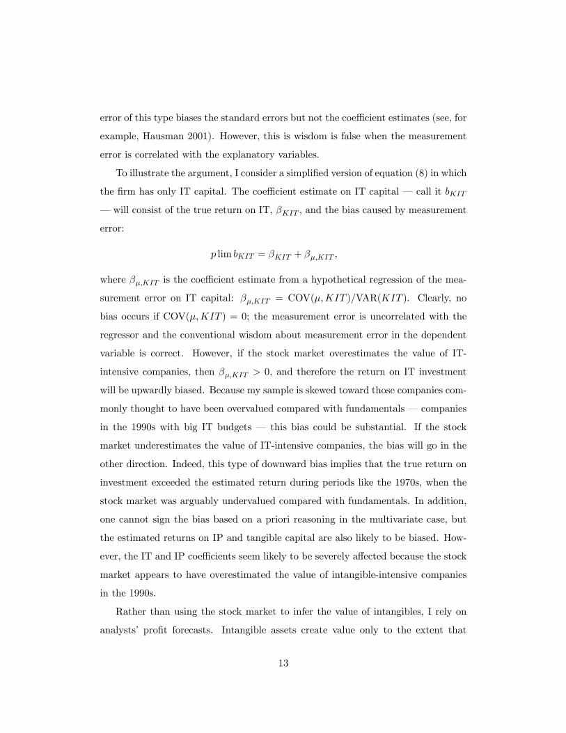
error of this type biases the standard errors but not the coefficient estimates (see, for

example, Hausman 2001). However, this is wisdom is false when the measurement

error is correlated with the explanatory variables.

To illustrate the argument, I consider a simplified version of equation (8) in which

the firm has only IT capital. The coefficient estimate on IT capital – call it bKIT

– will consist of the true return on IT, βKIT , and the bias caused by measurement

error:

p lim bKIT = βKIT + βµ,KIT ,

where βµ,KIT is the coefficient estimate from a hypothetical regression of the mea-

surement error on IT capital: βµ,KIT = COV(µ,KIT )/VAR(KIT ). Clearly, no

bias occurs if COV(µ,KIT ) = 0; the measurement error is uncorrelated with the

regressor and the conventional wisdom about measurement error in the dependent

variable is correct. However, if the stock market overestimates the value of IT-

intensive companies, then βµ,KIT > 0, and therefore the return on IT investment

will be upwardly biased. Because my sample is skewed toward those companies com-

monly thought to have been overvalued compared with fundamentals – companies

in the 1990s with big IT budgets – this bias could be substantial. If the stock

market underestimates the value of IT-intensive companies, the bias will go in the

other direction. Indeed, this type of downward bias implies that the true return on

investment exceeded the estimated return during periods like the 1970s, when the

stock market was arguably undervalued compared with fundamentals. In addition,

one cannot sign the bias based on a priori reasoning in the multivariate case, but

the estimated returns on IP and tangible capital are also likely to be biased. How-

ever, the IT and IP coefficients seem likely to be severely affected because the stock

market appears to have overestimated the value of intangible-intensive companies

in the 1990s.

Rather than using the stock market to infer the value of intangibles, I rely on

analysts’ profit forecasts. Intangible assets create value only to the extent that

13

they are expected to generate profits in the future. Professional analysts are paid

to forecast the future profits of the firms they track and leading analysts are paid

very well indeed for performing this role. Thus one can ask whether analysts are

forecasting profit growth in line with the intangible asset growth that seems to be

implied by stock market valuations. Though the popular press regularly lambastes

analysts for being far too optimistic, the answer is no.9 After introducing the data

in the next section, I show that analysts’ forecasts of future profits are informative.

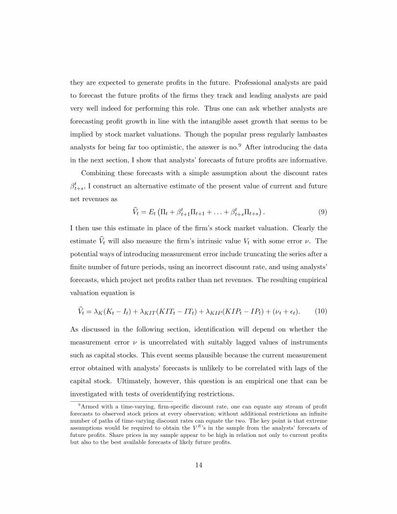
Combining these forecasts with a simple assumption about the discount rates

βtt+s, I construct an alternative estimate of the present value of current and future

net revenues as bVt = Et

¡Πt + βtt+1Πt+1 + . . .+ βtt+sΠt+s

¢. (9)

I then use this estimate in place of the firm’s stock market valuation. Clearly the

estimate bVt will also measure the firm’s intrinsic value Vt with some error ν. Thepotential ways of introducing measurement error include truncating the series after a

finite number of future periods, using an incorrect discount rate, and using analysts’

forecasts, which project net profits rather than net revenues. The resulting empirical

valuation equation is

bVt = λK(Kt − It) + λKIT (KITt − ITt) + λKIP (KIPt − IPt) + (νt + t). (10)

As discussed in the following section, identification will depend on whether the

measurement error ν is uncorrelated with suitably lagged values of instruments

such as capital stocks. This event seems plausible because the current measurement

error obtained with analysts’ forecasts is unlikely to be correlated with lags of the

capital stock. Ultimately, however, this question is an empirical one that can be

investigated with tests of overidentifying restrictions.9Armed with a time-varying, firm-specific discount rate, one can equate any stream of profit

forecasts to observed stock prices at every observation; without additional restrictions an infinitenumber of paths of time-varying discount rates can equate the two. The key point is that extremeassumptions would be required to obtain the V E ’s in the sample from the analysts’ forecasts offuture profits. Share prices in my sample appear to be high in relation not only to current profitsbut also to the best available forecasts of likely future profits.

14

3.2 Unobservable Productivity Shock

Despite some important differences, empirical valuation equations (8) and (10) re-

semble production functions. This similarity is unfortunate because, as Griliches

and Mairesse (1999) say, “In empirical practice, the application of panel methods to

micro-data have produced rather unsatisfactory results.” Mairesse and Hall (1996)

show that attempts to control for unobserved heterogeneity and simultaneity – both

likely sources of bias in the OLS results – have produced implausible estimates of

production function parameters. To be more specific, in my model I assume that the

unobservable productivity shock consists of a firm-specific, a time-specific, and an

idiosyncratic component. In this case, applying GMM estimators, which take first

differences to eliminate unobservable firm-specific effects and use lagged instruments

to correct for simultaneity in the first-differenced equations, has produced especially

unsatisfactory results.

Blundell and Bond (1998, 2000) show that these problems are related to the

weak correlation between the regressors and the lagged levels of the instruments.

This insignificant correlation results in weak instruments in the context of the first-

differenced GMM estimator. Bond and Blundell show that these biases can be

dramatically reduced by incorporating more informative moment conditions that

are valid under quite reasonable conditions. Essentially, their approach is to use

lagged first differences as instruments for equations in levels, in addition to the

usual lagged levels as instruments for equations in first differences. The result is the

so-called system-GMM estimator, which I use as the preferred estimator. I then use

DPD98 for GAUSS to perform the estimation (Arellano and Bond 1998).10

I conduct two types of diagnostic tests for the empirical models. First, I report

the p-value of the test proposed by Arellano and Bond (1991) to detect first- and

second-order serial correlation in the residuals. The statistics, which have a standard

10 In all specifications, I capture time effects by including year dummies in the estimated specifi-cations.

15

normal distribution under the null, test for nonzero elements on the second off-

diagonal of the estimated serial covariance matrix. Second, I report the p-value

of the Sargan statistic (also know as Hansen’s J-statistic), which is a test of the

model’s overidentifying restrictions; formally, it is a test of the joint null hypothesis

that the model is correctly specified and that the instruments are valid.

3.3 Limits of the Empirical Approach

If the GMM-based empirical approach is successfully implemented then that is the

end of the story in most applications. However, intangible assets pose a special prob-

lem. According to my model, intangibles are associated with specific investments,

but clearly that is not the whole story; sometimes intangibles are not associated

with any identifiable outlay. In that case, at least some of the intangibles end up

in the error term as an omitted variable or as part of the unobservable productivity

shock.

To fix ideas, let us suppose the fixed effect in the unobservable productivity shock

represents intangible capital. If the fixed effect embeds intangible capital in this way,

the econometric solution may be worse than the problem. In particular, taking first

differences will sweep out the effect of fixed intangible capital. As a result, the

possibility that intangible capital determines the level of the firm’s intrinsic value

will be completely missed.

Let us take another interesting example, MFP is normally thought of as a black

box but perhaps this box is full of what researchers mean by intangibles. Indeed,

many of the examples used to illustrate the role that intangibles play in organizations

have the flavor of MFP. That is, intangible capital comes from a good idea, like in

Dell’s case, selling computers over the Internet or from a unique corporate culture

created by a CEO like Jack Welch or Bill Gates. Nevertheless, most intangible assets

appear to be created by investment, as I argued in the introduction. After all, Dell

16

cannot sell computers over the Internet without its own computers, and Microsoft

spends more than $5 billion annually on R&D and advertising.

In summary, if one were to pursue an estimation strategy like GMM with instru-

ments that were arguably orthogonal to the error term, one might recover something

closer to the direct impact of any asset on market value. However, one would by

construction miss the role of omitted intangibles or intangibles that underlie the pro-

ductivity shock. Thus, such instrumental variable strategies could be informative,

but they could not provide the full set of answers about the role of intangibles.

In fact, Brynjolfsson, Hitt, and Yang (2000, 2002) have taken this argument one

step further: They say that the effect of intangible capital can be indirectly inferred

from OLS estimates of the return on IT capital. Two points are worth making about

this argument: the first is methodological and the second empirical.

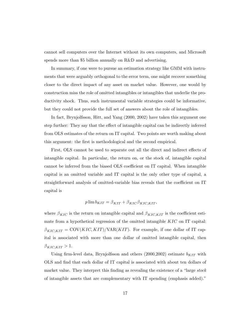
First, OLS cannot be used to separate out all the direct and indirect effects of

intangible capital. In particular, the return on, or the stock of, intangible capital

cannot be inferred from the biased OLS coefficient on IT capital. When intangible

capital is an omitted variable and IT capital is the only other type of capital, a

straightforward analysis of omitted-variable bias reveals that the coefficient on IT

capital is

p lim bKIT = βKIT + βKICβKIC,KIT ,

where βKIC is the return on intangible capital and βKIC,KIT is the coefficient esti-

mate from a hypothetical regression of the omitted intangible KIC on IT capital:

βKIC,KIT = COV(KIC,KIT )/VAR(KIT ). For example, if one dollar of IT cap-

ital is associated with more than one dollar of omitted intangible capital, then

βKIC,KIT > 1.

Using firm-level data, Brynjolfsson and others (2000,2002) estimate bKIT with

OLS and find that each dollar of IT capital is associated with about ten dollars of

market value. They interpret this finding as revealing the existence of a “large stock

of intangible assets that are complementary with IT spending (emphasis added).”

17

However, that conclusion depends on assumptions about little understood relation-

ships. Specifically, to say anything about the value of intangible capital, one must

know the return on IT capital. And to say anything about the return on intangibles

or the size of the stock of intangibles, one must break the value of intangible capital

into its constituent components. Brynjolfsson and others solve these problems by

assuming that adjustment costs are zero, in which case the returns to IT and in-

tangible capital are equal to unity (βKIT = βKIC = 1) and the stock of intangible

capital associated with IT capital can be backed out. According to this argument,

the stock market does not literally value one dollar of IT capital at ten dollars.

Rather, the estimate is a “marker” for the existence of a large stock of IT-related

intangibles.

The second concern is empirical: The results in Brynjolfsson and others (2000)

contradict the authors’ interpretation of the estimate on IT capital. When the

authors add a variable that measures organizational intangibles, ORG, to the re-

gressions, βKIT is almost totally unaffected.11 If the additional variable better

measures intangibles, as the authors argue persuasively, then bKIT should fall sig-

nificantly because it is a marker for intangibles. Because the estimate is about

unchanged, bKIT must be biased for another reason, like the stock market mismea-

surement or simultaneity bias that I have highlighted. If it is biased for another

reason, then one is wise to adopt an empirical technique that corrects for the bias.

4 Data

4.1 Sources and definitions

The limiting factor in our empirical analysis is the availability of data on IT out-

lays. For IT expenditures I use a dataset compiled by Lev and Radhakrishnan (this

11 In their subsequent paper, Brynjolfsson and others (2002) do not include the telling regressionfrom their first paper. Instead, they interact ORG with employment. Although the interpretationof the effect of ORG is complicated in this interaction, the take-away point remains the same: Theestimate on IT capital does not change significantly when ORG interacts with employment in theregression.

18

volume) from Information Week, which is in turn based on surveys by the Gart-

ner Group. The total sample is an unbalanced panel of firms that appeared in the

Information Week 500 list between 1991 and 1997 and for which Compustat and

I/B/E/S data are available.

The variables used in the empirical analysis are defined as follows:

• V E is the sum of the market value of common equity (defined as the number

of common shares outstanding multiplied by the end-of-fiscal-year common

stock price) and the market value of preferred stock (defined as the firm’s

preferred dividend payout divided by Standard & Poor’s preferred dividend

yield obtained from Citibase).

• bV is the present value of analysts’ profit forecasts. Let Πit and Πi,t+1 denote

firm i’s expected profits in periods t and t + 1, formed using beginning-of-

period information. Let git denote firm i’s expected growth rate of profits in

the following periods, formed using beginning-of-period information. Notice

that the stock market valuation of the firm, V E, is dated at time t − 1 sothat the market information set contains these forecasts. Then to calculate

the implied level of profits for periods after t + 1, I allow the average of Πit

and Πi,t+1 to grow at the rate git. Let this average be Πit.12

The resulting discounted sequence of profits defines bVit in the following way:bVit = Πit + βtΠi,t+1 + β2t (1 + git)Πit + β3t (1 + git)2Πit

+β4t (1 + git)3Πit + β5t

(1 + git)3Πit

r − g

12 In principle, the period for calculating bV should be infinity. However, analysts estimate g overa period of five years. Thus to match the period for which information exists, I set the forecasthorizon to five years. A terminal value correction accounts for the firm’s value beyond year five.The correction assumes that the growth rate for profits beyond this five-year horizon is equal tothat for the economy. Specifically, I create a growth perpetuity by dividing the last year of expectedearnings by (r − g) where I assume that r is the mean nominal interest rate for the sample periodas a whole (about 15%, which includes a constant 8 % risk premium) and g is the mean nominalgrowth rate of the economy for the sample period as a whole (about 6%).

19

The constant discount factor reflects a static expectation of the nominal inter-

est rate over this five-year period; that is, I use the Treasury bill interest rate

in year t (plus a fixed 8% risk premium as suggested by Brealey and Myers

(2000) among others).

• Dt is the book value of debt, which is the sum of short- and long-term oblig-

ations.

• Ct is net current assets, essentially cash on hand.

• I and K are capital expenditures and the current-cost net stock of property,

plant, and equipment (both excluding IT). In constructing the current-cost

stock, I follow the perpetual inventory method and use an industry-level rate

of economic depreciation derived from Hulten and Wykoff (1981).

• IT and KIT are IT expenditures and the current-cost net stock of IT. IT

outlays are from the Information Week survey. Again, in constructing the

current-cost stock, I follow the perpetual inventory method, and I use a de-

preciation rate consistent with annual economic depreciation of 40%.

• IP and KIP are IP expenditures and the current-cost net stock of IP. IP

expenditures are the sum of R&D and advertising. In constructing the current-

cost stock, I once more follow the perpetual inventory method, and I use a

depreciation rate consistent with annual economic depreciation of 25%.

The estimation sample includes all firms with at least four consecutive years of

complete data. Four years of data are required to calculate first differences and

to use lagged variables as instruments. I determine whether the firm satisfies the

four-year requirement after I delete several observations that appear to be recording

or reporting errors. Also, a few observations were deleted because bV < 0.13

13The data and programs for this study are available at www.insitesgroup.com/jason.

20

We turn now to a description of the sample (table 1). The first two rows of the

table define the different proxies for the intrinsic value of the firm. The total value

of the firm consists of three components: the return to equity holders, V E or bV ; thereturn to debt holders, D; and an adjustment for net current assets, C. At both the

mean and the median values, the stock-market-based value is about three-quarters

greater than the analyst-based value. Another notable feature of the sample is that

spending on IT and IP is a large fraction of total investment spending at the mean

and median values.

4.2 A Look at Analysts’ Forecasts

To lay the foundation for using the analyst-based proxy for the intrinsic value of the

firm, I compare the analysts’ forecasts of long-term growth, git, with realizations of

growth over a three-year period. My results show that analysts expected profits to

grow at an annual rate of 11.3% for the mean firm in my sample. Over a three-year

period, profits actually grew just a touch more slowly than estimated, at a rate of

11%.

A visual comparison of actual and expected profit growth is revealing (figure 1).

Three features of the data are apparent. First, analysts do not forecast negative long-

term growth. That practice is sensible because such forecasts would be equivalent

to saying that the company was essentially worthless. Second, analysts are loath

to forecast exceedingly high long-term growth rates – another sensible practice.

Few companies generate profit growth in excess of 30% and analysts cannot easily

identify ex ante those that may realize such growth. Finally, actual profit growth is

highly variable. Some companies grow at fast rates or suffer large retrenchments.

The OLS regression line describes the average relationship between the two vari-

ables. Actual and expected earnings growth are positively related – the slope of

the regression line is 0.74 with a standard error of 0.15 – but realized earnings

21

growth often differs widely from analysts’ expectations.14 Moreover, the forecasts

tend to be overly optimistic on average. In addition, analysts do not issue particu-

larly accurate long-range forecasts; evidently, a lot can happen to a company over a

three-year period, and most of what happens cannot be anticipated. However, the

key requirement for my purposes is not forecast accuracy but the ability of analysts’

forecasts to capture the expected future returns on which the firm’s investment de-

cisions are based. Judged according to this metric, analysts’ forecasts appear to be

reasonable and informative assessments about companies’ future prospects.

5 Empirical Results

Empirical results appear in two stages. I present OLS estimates of the empirical

valuation equations in levels and within-groups (table 2). After establishing that

these results are consistent with the sort of bias I have described, I present the

results from two GMM estimators (table 3). First, I present a standard estimator

that takes first differences in the empirical equations and uses lagged capital stocks as

instrumental variables. For reasons described in section 3.2, the coefficient estimates

are likely to be downwardly biased in this case. Second, I present results from the

system-GMM estimator. The diagnostic statistics indicate that system-GMM is

well-behaved when the analyst-based measure of intrinsic value is used and that the

results themselves are quite sensible.

5.1 OLS results

In the specification in the first column of table 2, the coefficient on IT capital

substantially and significantly exceeds unity, as does the coefficient on IP capital.

Meanwhile, the estimate of the return on tangible capital is significantly less than

14 I have left a few extreme observations out of the figure in order to maintain a 1:1 aspect ratio.However, in fitting the regression, I have included these observations.

22

unity.15 According to this first pass at the data, one dollar of IT capital is associated

with about two dollars of unmeasured intangibles and one dollar of IP capital is

associated with about one dollar of unmeasured intangibles. Thus, my basic results

parallel those reported by Brynjolfsson and others even though (1) I do not use the

same firms or estimation period, (2) I use different techniques for constructing the

capital stocks, and (3) I use different regressors.16

The pattern of estimates in column 1 is similar to that in column 2, where bVreplaces V E . In particular, whether one uses an analyst-based or a market-based

definition of intrinsic value does not make much difference when one estimates in

levels with OLS. However, the estimates on IT capital are considerably smaller in

columns 3 and 4, where net current assets are accounted for in valuing the firm.

Apparently, large IT capital stocks are associated with relatively abundant net cur-

rent assets. Microsoft, for example, has a large stock of IT and has amassed a huge

cash cushion on its balance sheet. When one ignores this relationship, the coefficient

on IT capital picks up both the effect of intangibles and the omitted effect of net

current assets. Thus, to develop an accurate picture of the role of IT capital, one

must define the value of the firm carefully.

So far the results have not controlled for unobserved heterogeneity. As a result,

the estimates are difficult to interpret because the firm-specific effect is surely cor-

related with contemporaneous capital investments. To sweep out the firm-specific

effect, I include within-group estimates presented in columns 5 and 6, which ex-

press all of the variables as deviations from within-firm means. In this case, the

coefficients on IT are significantly negative in both specifications, and the coeffi-

cients on the other types of capital appear downwardly biased in the final column.

These findings are not surprising because the capital stocks are highly persistent.

15Recall from the theoretical model that the beginning-of-period capital stocks belong on theright-hand side of the empirical valuation equation. According to equation (2), the beginning-of-period capital stocks are equal to the difference between the current capital stock and currentinvestment. Hence, the relevant regressors are (Kt − It) and so on.16 I could not investigate the effects of these differences because Brynjolfsson and his collaborators

declined to share their data.

23

Although unit-root tests are useless for short panels, the (unreported) AR(1) coef-

ficient estimates from regressions of the current capital stocks on their first lags are

all greater than 0.92. In such situations, the received wisdom from the literature

on production function estimation indicates that one should expect downward bias

from within-group estimates.17

5.2 GMM results

The GMM estimates are useful because the within-group results do nothing to con-

trol for simultaneity bias. Such bias must be important because the value of the firm

(no matter how it is measured) and its investment policy are jointly determined.

To see the intuition behind this point, compare the empirical valuation equation

with an empirical investment equation based on Tobin’s Q. In the current setup,

the firm’s intrinsic value is a function of the capital stock and investment, whereas

the reverse is true in an equation that relates the investment rate to Tobin’s Q.

Put simply, increases in market value may cause investment in IT (and other types

of capital) but the reverse may be true, too. To deal with simultaneity bias (and

eliminate the firm-specific effect at the same time), I estimate the first-differenced

empirical valuation equations with GMM, using lagged levels of the capital stocks

as instruments (table 3).

Looking first at the Sargan test, we see that the p-values in columns 1 and 2 of the

table do not indicate a decisive rejection of the model’s overidentifying restrictions.

This result does not mean, however, that the instruments are informative. Indeed,

in unreported results, I confirm that one cannot reject weak instruments when using

the partial R2 or first-stage F -statistic as criteria. If the instruments used in the

first-differenced equations are weak, then the results should be biased in the direction

17 In fact, it is not unusual for production function estimates of the capital share to go from 0.3in levels to negative values in within-groups. By comparison, the magnitude of the bias in table 2may seem surprisingly large, but one should keep in mind that production functions are estimatedin logs.

24

of within-groups.18 Indeed, a comparison of columns 1 and 2 of table 3 with columns

5 and 6 of table 2 shows that the direction and magnitude of the bias are similar in

the first-differenced and within-group estimates.

To address concerns about weak instruments, I use the system-GMM estimator

in columns 3 and 4 of table 3. The Sargan test indicates that the model using

V E is decisively rejected while the one using bV is not. This result suggests that

the instruments are correlated with the market’s, but not with the analysts’, mis-

measurement of companies’ intrinsic values. Why might this correlation occur? As

I have argued, intangibles are difficult to value. If, say, the lagged change in the

stock of intangibles is correlated with the extent to which the market overstates the

firm’s intrinsic value, then the system-GMM estimator will tend to be rejected. In

contrast, for reasons I have discussed, we have little reason to worry that analysts’

forecast errors are correlated with the lagged change in the stock of intangibles, and

the Sargan test supports this conjecture. Therefore, my preferred estimates use the

analyst-based measure of the firm’s intrinsic value.

In column 4, the coefficient estimates on tangible and IP capital are insignifi-

cantly different from unity (although they are significantly different from zero), and

the coefficient on IT capital is significantly greater than unity. Taken at face value,

the coefficient on IT capital implies that organizational capital earns a 72% annual

rate of return, a figure that may seem excessive. However, two points are worth

nothing. First, the evidence of excess returns is statistically weak because the 95%

confidence interval encompasses returns as low as 7%. Second, in my model the

return on IT capital includes the effect of adjustment costs; indeed, that is how

organizational capital is defined in equation (6). This possibility is seldom noted

18The technical explanation for this statement depends on two things. First, weak instrumentswill bias 2SLS in the direction of OLS. Second, the first-differenced GMM estimator coincides with a2SLS estimator when the fixed effects are removed with the orthogonal deviations transformation;and OLS transformed to orthogonal deviations coincides with within-groups. Therefore, weakinstruments will bias this particular 2SLS estimator (which coincides with first-differenced GMM)in the direction of within-groups.

25

because researchers usually estimate the return on IT with a static production func-

tion, which assumes that capital is in a steady-state equilibrium so that adjustment

costs are zero by construction.19

The coefficient on IP capital is less than unity, a result consistent with earlier

findings that R&D earns a somewhat less than normal rate of return (see, for exam-

ple, Hall 1993b). Perhaps firms cannot reap the full benefit of their IP investments

because of the nonexclusive nature of some types of R&D (see, for example, Griliches

1979; Jaffe 1986; Bernstein and Nadiri 1989). However, one must exercise caution

in drawing such a conclusion because the 95% confidence interval encompasses re-

turns as large as 20%, a result more in line with the recent findings in Hand (2002).

Finally, the estimate on tangible capital (excluding IT) is slightly less than unity.

This outcome is consistent with lower rates of return on these types of capital and

with recent studies in which estimated adjustment costs are quite modest in size

(see, for example, Bond and Cummins 2000a).

6 Conclusion

The dramatic rise of the stock market in the 1990s led some observers to conclude

that intangible capital was an increasingly important contributor to the bottom line

at many companies. However, the abrupt and sustained decline in the stock market

that began in 2000 seemed to suggest just the opposite. This reversal highlighted

the desirability of alternative measurement strategies that would distinguish between

the gyrations of the stock market and the value created by intangibles.

My empirical approach offers such an alternative strategy and provides a differ-

ent perspective about what intangibles are and how researchers can estimate their

19To see the implications of my approach in the context of a production function, notice thatthe marginal product of capital in my model is equal to the traditional user cost plus adjustmentcosts. For example, abstracting from taxes and setting the price of capital equal to unity, I calculateequilibrium condition in my model as ∂Π

∂KIT = r + δKIT +∂C

∂KIT . As long as adjustment costs arepositive, the estimated return on capital can exceed (r + δKIT ), the usual required rate of returnunder the equilibrium condition in production function framework.

26

return. In my model, intangible capital is not a distinct factor of production as is

physical capital or labor; indeed, I assume that intangibles, unlike a computer or a

college graduate, cannot be purchased in a market. Nor are intangibles some kind of

relabeled MFP. Rather, intangible capital is the “glue” that creates value from the

usual factor inputs. This perspective naturally suggests an empirical model in which

intangible capital is defined in terms of adjustment costs. As such, intangibles are

the difference between the value of installed inputs and that of uninstalled inputs.

In my empirical approach, I use two proxies for the intrinsic value of the firm,

one based on the firm’s stock market value and the other based on analysts’ profit

forecasts. In addition, I use a GMM estimation technique to control for unobserved

heterogeneity and simultaneity bias in specifications with nearly integrated regres-

sors. Using the analyst-based proxy and the GMM technique, I find no evidence

of economically important intangibles associated with investment in intellectual

property or physical capital apart from IT. However, my estimates suggest that

organizational capital created by information technology generates a 72% annual

rate of return.

These findings come with a caveat. Controlling for simultaneity bias and unob-

served heterogeneity removes intangibles that may have been swept into the error

term, either as omitted variables or as part of the unobservable productivity shock.

Nevertheless, alternative empirical approaches are unpalatable to say the least. In-

deed, my OLS estimates seem to imply a strong role for intangibles, but they are

unreliable because the value of the firm and its investment policy are jointly de-

termined. In the end, how best to characterize the heterogeneity across firms and

what role intangibles play remain open questions. Are intangibles part of the un-

observable productivity shock? Are intangibles some fixed (or quasi-fixed) factor

that interacts in complex ways with other inputs? The answers to these questions

remain unresolved.

27

Finally, I consider whether my approach suggests ways to incorporate intangible

capital into national income accounting. At a basic level, the implications are not

encouraging. Factor inputs in the national accounts have prices, but such prices

are often difficult to measure accurately. In contrast, my approach starts with the

assumption that intangibles are nearly impossible to value as standalones. In par-

ticular, intangibles have unobservable shadow prices that depend on expectations.

This setup makes the return on intangibles impossible to measure directly and un-

certain by construction. These two features render intangible capital particularly

ill suited to national income accounting. Nevertheless, my approach does suggest a

road map for improving the national accounts. A key ingredient for better under-

standing the scope of intangibles is detailed data on the types of outlays that are

closely connected with intangibles. In this regard, the national accounts could be

considerably improved. I focused on IT, R&D, and advertising but it would be de-

sirable to have data on other types of outlays, such as education, on-the-job training

programs, and the like.

28

References

Arellano, Manuel and Stephen R. Bond (1991). Some tests of specification for panel

data: Monte Carlo evidence and an application to employment equations. Re-

view of Economic Studies 58(2): 277—97.

Arellano, Manuel and Stephen R. Bond (1998). Dynamic panel data estimation using

DPD98: A guide for users. Manuscript, Oxford University.

Baily, Martin Neil (1981). Productivity and the services of capital and labor. Brook-

ings Papers on Economic Activity 1981(1): 1—50.

Bernstein, Jeffrey I. and M. Ishaq Nadiri (1989). Research and development and

intra-industry spillovers: An empirical application of dynamic duality. Review

of Economic Studies 56(2): 249—69.

Blundell, Richard and Stephen R. Bond (1998). Initial conditions and moment

restrictions in dynamic panel data models. Journal of Econometrics 87(1): 115—

43.

Blundell, Richard and Stephen R. Bond (2000). Gmm estimation with persis-

tent panel data: An application to production functions. Econometric Re-

views 19(3): 321—40.

Bond, Stephen R. and Jason G. Cummins (2000a). Noisy share prices and the Q-

model of investment. Manuscript, New York University.

Bond, Stephen R. and Jason G. Cummins (2000b). The stock market and investment

in the new economy: Some tangible facts and intangible fictions. Brookings

Papers on Economic Activity 2000(1): 61—124.

Brealey, Richard A. and Stewart C. Myers (2000). Principles of Corporate Finance

(6th ed.). New York: McGraw-Hill.

Bresnahan, Timothy, Eric Brynjolfsson, and Lorin Hitt (2002). Information tech-

nology, workplace organization, and the demand for skilled labor: Firm-level

evidence. Quarterly Journal of Economics 117(2): 339—76.

29

Brynjolfsson, Eric, Lorin Hitt, and Shinkyu Yang (2000). Intangible assets: How

the interaction of information technology and organizational structure affects

stock market valuations. Manuscript, MIT.

Brynjolfsson, Eric, Lorin Hitt, and Shinkyu Yang (2002). Intangible assets: Comput-

ers and organization capital. Brookings Papers on Economic Activity 2002(1):

137—81.

Campbell, John Y., Andrew W. Lo, and A. Craig MacKinlay (1997). The Econo-

metrics of Financial Markets. Princeton: Princeton University Press.

Griliches, Zvi (1979). Issues in assessing the contribution of research and develop-

ment to productivity growth. Bell Journal of Economics 10(1): 92—116.

Griliches, Zvi and Jacques Mairesse (1999). Production functions: The search for

identification. In S. Strom (Ed.), Econometrics and Economic Theory in the

20th Century: The Ragnar Frisch Centennial Symposium. Cambridge: Cam-

bridge University Press.

Hall, Bronwyn H. (1993a). Industrial research during the 1980s: Did the rate of

return fall? Brookings Papers on Economic Activity 1993(2): 289—343.

Hall, Bronwyn H. (1993b). The stock market’s valuation of R&D investment during

the 1980s. American Economic Review 84(1): 1—12.

Hall, Robert E. (2001). The stock market and capital accumulation. American Eco-

nomic Review 91(6): 1185—1202.

Hand, John R. M. (2002). The profitabillity and returns-to-scale of expenditures

on intangibles made by publically-traded U.S. firms, 1980-2000. Manuscript,

University of North Carolina.

Hausman, Jerry A. (2001). Mismeasured variables in econometric analysis: Problems

from the right and problems from the left. Journal of Economic Perspec-

tives 15(4): 57—67.

30

Hayashi, Fumio and Tohru Inoue (1991). The relation between firm growth and Q

with multiple capital goods: Theory and evidence from panel data on Japanese

firms. Econometrica 59(3): 731—753.

Hempell, Thomas (2003). Do computers call for training? Firm-level evidence on

complementarities between ICT and human capital investments. Manuscript,

ZEW.

Hulten, Charles R. and Frank Wykoff (1981). Measurement of economic deprecia-

tion. In C. R. Hulten (Ed.), Depreciation, Inflation, and the Taxation of Income

from Capital. Washington: Urban Institute.

Jaffe, Adam (1986). Technological opportunity and spillovers of R&D: Evidence from

firms’ patents, profits and market value. American Economic Review 76(4):

984—1001.

Kiley, Michael T. (2000). Stock prices and fundamentals in a production economy.

Manuscript, Board of Governors of the Federal Reserve System.

Lev, Baruch (2001). Intangibles: Management, Measurement, and Reporting. Wash-

ington, D.C.: Brookings Institution Press.

Mairesse, Jacques and Bronwyn H. Hall (1996). Estimating the productivity of

research and development: An exploration of GMM methods using data on

French and United States manufacturing firms. NBERWorking Paper No. 5501.

McGrattan, Ellen R. and Edward C. Prescott (2000). Is the stock market overval-

ued? Manuscript, Federal Reserve Bank of Minneapolis.

Nakamura, Leonard (1999). Intangibles: What put the new in the new economy?

Federal Reserve Bank of Philadephia Business Review July/August: 3—16.

Prescott, Edward C. and Michael Visscher (1980). Organization capital. Journal of

Political Economy 88(3): 446—61.

Shiller, Robert J. (2000). Irrational Exuberance. Princeton: Princeton University

Press.

31

Siegel, Jeremy (1998). Stocks for the Long Run: The Definitive Guide to Financial

Market Returns and Long-term Investment Strategies (2nd ed.). New York:

McGraw-Hill.

32

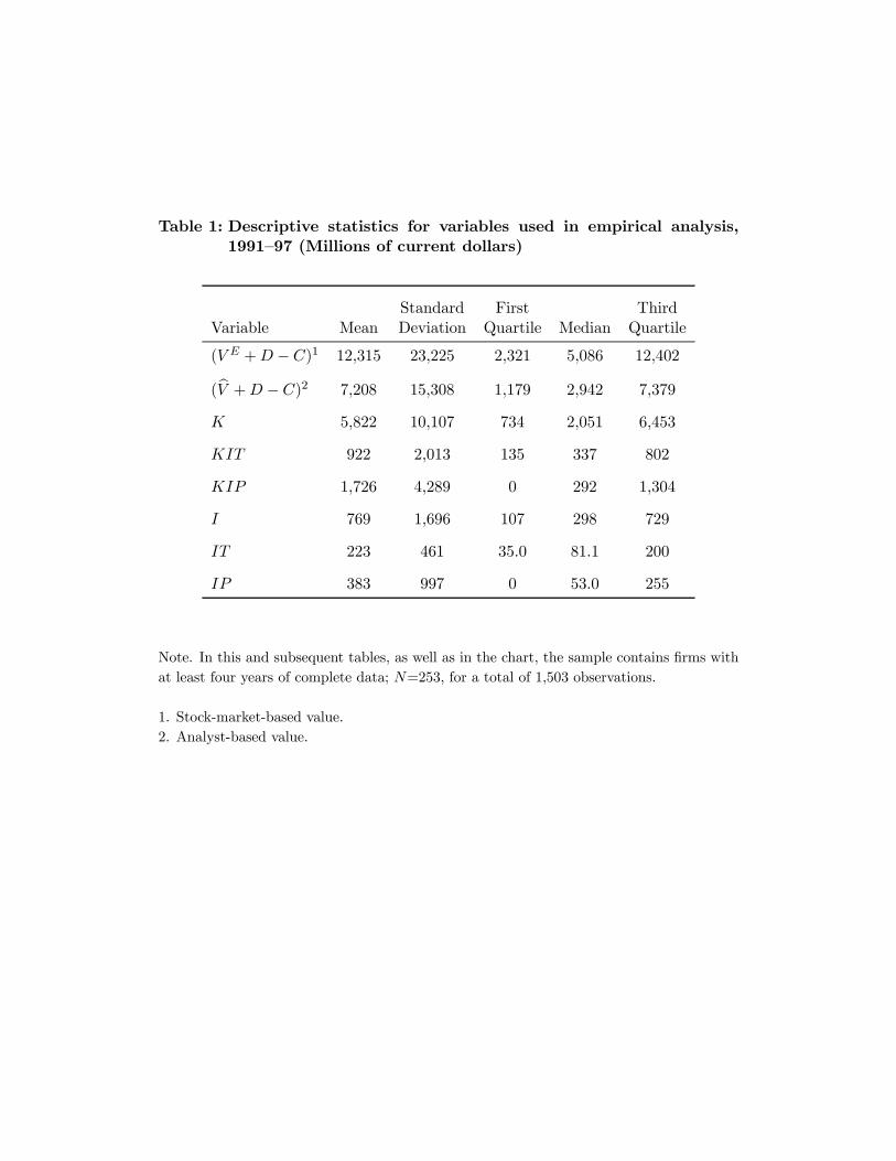
Table 1: Descriptive statistics for variables used in empirical analysis,1991—97 (Millions of current dollars)

Standard First ThirdVariable Mean Deviation Quartile Median Quartile

(V E +D − C)1 12,315 23,225 2,321 5,086 12,402

(bV +D − C)2 7,208 15,308 1,179 2,942 7,379

K 5,822 10,107 734 2,051 6,453

KIT 922 2,013 135 337 802

KIP 1,726 4,289 0 292 1,304

I 769 1,696 107 298 729

IT 223 461 35.0 81.1 200

IP 383 997 0 53.0 255

Note. In this and subsequent tables, as well as in the chart, the sample contains firms withat least four years of complete data; N=253, for a total of 1,503 observations.

1. Stock-market-based value.2. Analyst-based value.

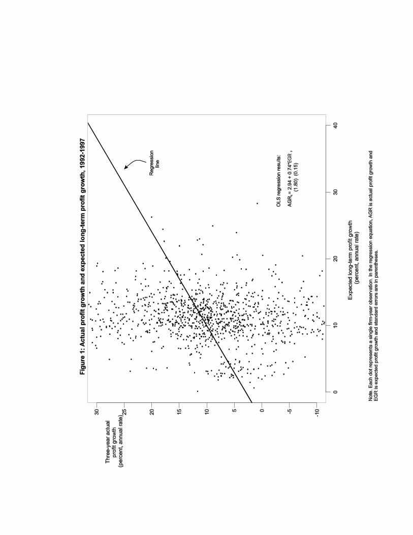
Table 2: OLS estimates of the valuation equations, 1992—97

Level Within-group

Dependent variable Dependent variable

(V Et +Dt) (bVt +Dt) (V E

t +Dt − Ct) (bVt +Dt − Ct) (V Et +Dt − Ct) (bVt +Dt − Ct)

(1) (2) (3) (4) (5) (6)

(Kt − It) 0.753 0.482 0.821 0.550 0.892 0.182(0.075) (0.064) (0.064) (0.048) (0.216) (0.169)

(KITt − ITt) 3.19 3.14 1.97 1.91 -6.67 -8.63(0.491) (0.416) (0.415) (0.316) (0.836) (0.656)

(KIPt − IPt) 2.07 1.54 1.84 1.31 2.67 0.383(0.211) (0.179) (0.179) (0.136) (0.685) (0.537)

Diagnostic Tests (p-values)

Serial correlation1

First-order 0.070 0.066 0.143 0.169 0.930 0.886Second-order 0.086 0.086 0.171 0.214 0.245 0.317

R2 0.451 0.401 0.474 0.457 0.107 0.171

Note. Year dummies are included (but not reported) in all specifications. Robust standard errors oncoefficients are in parentheses. For estimation N=253 but we drop the first year, leaving a total of 1,250observations.

1. The test for serial correlation in the residuals is asymptotically distributed as N(0,1) under the null of noserial correlation.

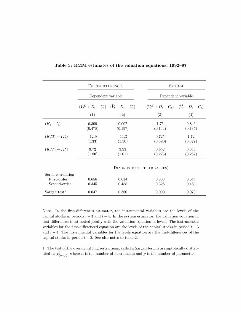
Table 3: GMM estimates of the valuation equations, 1992—97

First-differences System

Dependent variable Dependent variable

(V Et +Dt − Ct) (bVt +Dt − Ct) (V E

t +Dt − Ct) (bVt +Dt − Ct)

(1) (2) (3) (4)

(Kt − It) 0.399 0.007 1.75 0.846(0.478) (0.197) (0.144) (0.135)

(KITt − ITt) -12.9 -11.3 0.725 1.72(1.33) (1.30) (0.390) (0.327)

(KIPt − IPt) 9.72 3.93 0.652 0.684(1.80) (1.01) (0.273) (0.257)

Diagnostic tests (p-values)

Serial correlationFirst-order 0.656 0.634 0.883 0.644Second-order 0.345 0.488 0.326 0.463

Sargan test1 0.047 0.360 0.000 0.073

Note. In the first-differences estimator, the instrumental variables are the levels of thecapital stocks in periods t− 3 and t− 4. In the system estimator, the valuation equation infirst-differences is estimated jointly with the valuation equation in levels. The instrumentalvariables for the first-differenced equation are the levels of the capital stocks in period t− 3and t− 4. The instrumental variables for the levels equation are the first-differences of thecapital stocks in period t− 2. See also notes to table 2.

1. The test of the overidentifying restrictions, called a Sargan test, is asymptotically distrib-uted as χ2(n−p), where n is the number of instruments and p is the number of parameters.