a new approach to history matching of water driven … · a new approach to history matching of ......
TRANSCRIPT

i
A New Approach to History Matching of Water Driven Oil Reservoirs
A DISSERTATIONSUBMITTED TO THE
DEPARTMENT OF MINERAL RESOURCES AND PETROLEUM ENGINEERING AND THE COMMITTEE ON GRADUATE STUDIES OF THE
UNIVERSITY OF LEOBEN, AUSTRIA,IN PARTIAL FULLFILLMENT OF THE REQUIREMENTS FOR THE DEGREE OF
"DOKTOR DER MONTANISTISCHEN WISSENSCHAFTEN"
written by
Dipl.-Ing. Fathe A.S Abrahem October 2009
Advisor:
Em.O..Univ.Prof. Dipl.IngDr.Dr.h.c. Zoltán E. Heinemann

ii

iii
Affidavit
I declare in lieu of oath that I did this work by myself using only literature, cited in thetext and listed in the end of this volume.
__________________________
Dipl.-Ing. Fathe A.S Abrahem
Leoben, October 2009

iv
Dedication
First of I all I would like to say thanks to my GOD, for everything, and I would like todedicate this work firstly to my family, secondly to my beloved country and loved ones ofeach.

v
Acknowledgment
The author thanks em.O.Univ.Prof.Dipl.-Ing.Dr.Dr.h.c. Zoltan Heinemann to teach andguide him during his Master of Science and Doctorate study in Petroleum Engineeringover the years 2004-2009. The research topic awarded by Prof. Heinemann was not onlyscientifically exciting but with high practical importance for the author’s country theGreat Arabian Jamahariya. The author thanks for continuous and intensive support byProf. Heinemann and his colleagues, Dr. Georg Mittermeir and Dr. Andreas Harrer. Theauthor is aware that to be the MS and PhD student of one of the winner of John FranklinCarrl Award confer him a particular state in the petroleum industry and science and he willtry to be worthy to his sperendipity.
The author would like to thank so much NOC Libya and ZOC for granting permission forthis study; furthermore thanks to AGOCO Libya for the permission using the data of theKOTLA field in this work, which is highly appreciated.
The author is grateful to the management and staff of OMV Libya for sponsoring hisstudy, especially to Dipl.Ing. Walter Ondracek.
Special thanks goes to Heinemann Oil GmbH and its Chief Executive Officer Dr. GaborHeinemann for assuring office space and facilities over three years in Leoben. Also Iwould like to thank, the entire staff for the cooperation without mentioning any personbecause everyone was very kind.
The author thanks Professor Dr.Stephan Matthäi for reading the work and giving criticalcomments that helped to increase the quality of the dissertation.

vi
Kurzfassung
Ein neuer Ansatz des History Matching für Öllagerstätten mit Wassertrieb
von Dipl.Ing.Fathe A.S.Abrahem
In dieser Dissertation wird eine neue Methode des History Matching präsentiert. Ziel derkonventionellen Methode ist es ein Lagerstättenmodell zu erstellen, das die historischenDaten, wie Förderraten, Bohrlochdrücke, Wasseranteil und GOR über die gesamteProduktionszeit mit vorgegebenen Bohrlöchern simulieren kann. Bei der hierpräsentierten Methode wird das Lagerstättenmodell als gegeben angenommen, dieBohrlöcher im Modell werden automatisch platziert, wobei diese Pseudo-Bohrlöchernicht unbedingt den "echten" Bohrlöchern entsprechen müssen, der Materialflussentspricht zu jedem Zeitpunkt dem historischen. Wenn es nicht möglich istPseudo-Bohrlöcher im Modell zu platzieren ist das statische Modell falsch und mussausgetauscht werden. Stochastische Realisationen können bereits von Anfang anüberprüft werden. Zusätzliche Bohrlöcher injizieren Wasser an den Modellgrenzen,wodurch der mittlere Druck in jeder Region im Modell dem historischen Druckentspricht. Nachdem die historischen Raten und Drücke mithilfe der Pseudo-Bohrlöchernachgestellt werden können werden die Pseudo-Bohrlöcher durch die echten Bohrlöcherersetzt. Die Lagerstätteneigenschaften und die Perforationen werden schrittweiseaufeinander abgestimmt. Dieses Tuning erfolgt teilweise automatisch, teilweise händisch,wobei das Programm Vorschläge für den Softwareanwender ausschreibt. Der HistoryMatching Prozess ist abgeschlossen sobald alle Pseudo-Bohrlöcher durch "echte" ersetztworden sind.
Pars Reservoir Simulator (PRS) ist eine nicht-kommerzielle, benutzerfreundlicheLagerstättensimulationssoftware, welche einerseits unabhängig, andererseits alsVorprozessor von ECLIPSE benutzt werden kann. Dem ECLIPSE Input werden einigeKommandozeilen hinzugefügt. PRS generiert eine modifizierte SCHEDULE Datei, dieim folgenden ECLIPSE Simulationslauf verwendet wird. Diese enthält die aktuellenEinstellungen der Pseudo-Bohrlöcher sowie die Parameter für analytische Fetkovitchoder Carter-Tracey Grundwasserleiter Modelle, welche die Wasserinjektion an denModellgrenzen ersetzen.
Die vorliegende Arbeit beinhaltet neben den für PRS entwickelten Methoden undAlgorithmen ein Fallbeispiel einer Lagerstätte mit 700 Mio. stb Originalvolumen, 60Bohrlöchern und einer Produktionszeit von mehr als 45 Jahren.
vii
Abstract
A New Approach to History Matching of Water Driven Oil Reservoirs
by Fathe A.S. Abrahem
This dissertation presents a new technique for history matching. In the conventionalapproach the model wells are fixed and one seeks for a reservoir model in which theyprovide the historical rates, well pressures, WC and GOR over the entire time. Thepresented method does the opposite, the reservoir model is given and the computer placesautomatically wells which can do what they should do. These pseudo wells are perhaps atdifferent location and open also other layers than the real wells but the overall materialtransfer will be correct for all the time. If such wells can not be placed, then the staticmodel is fundamentally wrong and must be replaced. Stochastic realisations can bescreened at this level already. Supplementary pseudo wells inject water to the modelboundaries, assuring that the average pressure in any chosen region closely follows thehistorical pressure. After the global match succeeded, the pseudo wells are shifted towardthe real ones and the reservoir and perforation properties will be tuned step by step, partlyautomatically partly manually. For the second one the procedure writes suggestions forthe user. The HM is completed after all pseudo wells are replaced by the real wells.
Pars Reservoir Simulator (PRS) is a fully developed not commercial user friendly toolwhich can be used stand alone but also as a certain kind of pre-processor to ECLIPSE. Thetool needs some command lines added to ECLIPSE input only. PRS write out a modifiedSCHEDULE file containing the actual settings of the pseudo wells and the parameters forthe Fetkovich and Carter-Tracy analytical aquifer models (replacing the boundaryinjections) for the next ECLIPSE run.
Beside the methods and algorithm used in PRS the work present a full field application.The reservoir contains 700 MMstb OOIP and it was operated by 60 wells over 45 years.

viii
NotesThe dissertation was issued in two versions, both in 5 numbered copies. The first one isthe original version containing proprietary data and information of the followingcompanies:
National Oil Company, Tripoli, LibyaArabian Gulf Oil Company, Benghazi, LibyaHeinemann Oil Gmbh, Leoben, Austria
The second version was neutralized; numbers as geographic coordinates, reserves,production data, etc. has been erased and field, formation, etc. names has been changed.These changes do not hamper the scientific evaluation of the work.
ECLIPSE, CPS-3, GeoFrame 3D and Petrel are copyrighted by Schlumberger Ltd.
STARS, IMEX and WinProp are copyrighted by CMG (Computer Modelling Group Ltd.)
PRS is copyrighted by Heinemann Oil Gmbh
SURE,SUREGrid are copyrighted by SST Simulation Software Technology GmbH
1
Chapter 1
Introduction ................................................................................................................11.1 Motivation of Work .............................................................................................................11.2 The Objectives .....................................................................................................................21.3 The Approach .......................................................................................................................41.4 Software Tools .....................................................................................................................51.5 Outline ..................................................................................................................................61.6 Scientific Achievements and Technical Contributions ........................................................71.7 Publications of the Author ...................................................................................................8
Chapter 2
Notes to Reservoir Modeling ....................................................................................92.1 Introduction ..........................................................................................................................92.2 Simulation versus Mathematical Modeling .......................................................................102.3 History Matching ...............................................................................................................12
2.3.1 What is It? ............................................................................................................122.3.2 Quality of History Match .....................................................................................152.3.3 Automated and Computer Assisted History Matching ........................................18
2.4 Aquifer Models ..................................................................................................................202.4.1 Introduction and background information to Aquifer Modeling .........................202.4.2 Gridded Aquifer Models ......................................................................................212.4.3 Analytical Aquifer Modeling ...............................................................................21
2.4.3.1 Aquifer Models.......................................................................................212.4.3.2 Inflow into the Artificial Boundaries......................................................242.4.3.3 Implementation in Grid Model ...............................................................262.4.3.4 Average Boundary Pressure ...................................................................272.4.3.5 Distribution of a Given Rate between the Outer Boundary Blocks........28
2.5 Target Pressure Method .....................................................................................................292.5.1 Previous Works ....................................................................................................292.5.2 Identification of the Optimal Analytical Aquifer Model .....................................322.5.3 Application of TPM to TPPM .............................................................................33
2.5.3.1 Experiences.............................................................................................332.5.3.2 Improvements .........................................................................................332.5.3.3 Fetkov Test Model..................................................................................34
Chapter 3
Target Pressure and Phase Method ........................................................................393.1 Definition of TPPM ...........................................................................................................393.2 Elements of TPPM .............................................................................................................423.3 The TPPM Work Flow .......................................................................................................433.4 Well by Well Matching ......................................................................................................47

2
Chapter 4
The Field Case ..........................................................................................................494.1 Field Data and Project Objectives ......................................................................................494.2 Summary of the Geological Model ....................................................................................50
4.2.1 Structure of the reservoir .....................................................................................504.2.2 Reservoir parameters ...........................................................................................524.2.3 Grid and Upscaling ..............................................................................................53
4.3 Field Production .................................................................................................................574.4 Reservoir Pressure ..............................................................................................................594.5 Water Influx .......................................................................................................................614.6 Extracted Single Well Models ...........................................................................................61
Chapter 5
Validation of the Target Pressure and Phase Method ..........................................655.1 Introduction ........................................................................................................................655.2 Well Models .......................................................................................................................66
5.2.1 Inflow performance ..............................................................................................665.2.2 Productivity Index ................................................................................................695.2.3 Estimation of perforation rates .............................................................................695.2.4 Crossflow .............................................................................................................71
5.3 Pseudo Wells ......................................................................................................................725.3.1 Setting of pseudo wells ........................................................................................72
5.4 Single Well Modeling ........................................................................................................735.4.1 Experiment with constant rate .............................................................................755.4.2 Assessment of the Analytical Aquifer .................................................................785.4.3 Experiments with Historical Production Rate ......................................................80
5.5 Applicability of TPPM to Stratified Reservoirs .................................................................835.5.1 The Objective .......................................................................................................835.5.2 Model Setup .........................................................................................................84
Chapter 6
Full Field Application of TPPM .............................................................................916.1 Introduction ........................................................................................................................916.2 History Matching Workflow ..............................................................................................926.3 Initialization .......................................................................................................................94
6.3.1 Structural Modifications ......................................................................................956.3.1.1 Faults.......................................................................................................956.3.1.2 Aquifer Parameters .................................................................................966.3.1.3 Porosity Alterations of the HM model....................................................966.3.1.4 NTG Alterations in the HM model .........................................................976.3.1.5 Rock region distribution in the HM model.............................................97

3
6.3.1.6 Permeability Alterations in the HM model.............................................986.4 Results of the History Match ...........................................................................................100
6.4.1 Global Match .....................................................................................................1016.4.2 Well-by-Well Match ..........................................................................................1026.4.3 Saturation distribution in the Reservoir .............................................................103
Chapter 7
Closing Remarks ....................................................................................................106
Chapter 9
Nomenclature ......................................................................................................... 111
1
List of FiguresFigure 2.1: Use mathematical models in analytical and simulation mode (after Z.E.Heinemann27) 11Figure 2.2: The nature of numerical simulation (after Z.E.Heinemann27) ........................................12Figure 2.3: Standard Simulation Workflow.......................................................................................13Figure 2.4: New Simulation Workflow .............................................................................................14Figure 2.5: Validation of a dynamic resevoir model in a conventional approach .............................15Figure 2.6: Both cumulative production and trend fit (well C51_VR17)..........................................16Figure 2.7: Cumulative production failed, trend fits (well C38_VR5)..............................................16Figure 2.8: Cumulative production fits, trend failed (well C23_VR)................................................17Figure 2.9: History match of the well failed (well C35_VR4) ..........................................................17Figure 2.10:Simulation model with gridded aquifer (after Heinemann22) ........................................21Figure 2.11:Grid model of a Productive Area (from HOT SURE manual31) ....................................26Figure 2.12:Segmented Outer Boundaries and appropriate Target Areas (from Mittermeir44) ........27Figure 2.13:Comparison of the result of the TPM calculation with the measured data (from
Mittermeir44) ...................................................................................................................31Figure 2.14:Boundary pressure and injected water into the artificial outer boundary (from
Mittermeir44) ...................................................................................................................31Figure 2.15:: Cross-section view of Fetkov Test Model showing well position and boundary location
(exaggeration = 50). ........................................................................................................34Figure 2.16:: Cross-section view of Fetkov Test Model showing pressure gradient between water pro-
ducer and analytical aquifer at 1988/01/01 (exaggeration = 50).....................................35Figure 2.17:Comparison of average reservoir pressure calculated with ECLIPSE and PRS (before im-
provement) at a time step length of DT = 31 days. .........................................................37Figure 2.18:Comparison of average reservoir pressure calculated with ECLIPSE and PRS (before im-
provement) at a time step length of DT = 1 days. ...........................................................37Figure 2.19:Comparison of water encroachment as a function of time for Fetkov Test model before
improvement of PRS. ......................................................................................................38Figure 2.20:Comparison of average reservoir pressure calculated with ECLIPSE and PRS (after im-
provement) at a time step length of DT = 31 days. .........................................................38Figure 3.1: Principal of the Target Pressure Method. Idea and development by Pichelbauer, Mitter-
meir and Heinemann51,42,44...........................................................................................40Figure 3.2: Concept of Target Pressure and Phase Method. TPPM assignes the phase production rates
to well spots and not to the wells. Idea from Abrahem...................................................40Figure 3.3: Difference between the conventional and TPPM history matching approach. The Target
Pressure Method (TPM) is part of TPPM. ......................................................................41Figure 3.4: Target Pressure and Phase Method dicectly screens the geological realisations. ...........41Figure 4.1: 3-D view of the structural configuration interpreted for the northern area of the CON55
Field (after Davis and Egger13). ......................................................................................51Figure 4.2: Wells, volume region, boundary and fault names of CON55 Field (#W block) (from
Mittermeir41, modified by the author).............................................................................52Figure 4.3: East-west cross section through wells C16 and C2 showing porosity of the geological
model (top) and the simulation model (after Davis and Egger13, modified by the author). ........................................................................................................................................54
Figure 4.4: Cross section through wells C8, C21, C19 and C6 showing log derived water saturation of the geological model (top), showing log derived water saturation of the upscaled geo-

2
logical model and water saturation of the equilibrium initialization in the simulation mod-el (after Davis and Egger13, modified by the author)......................................................56
Figure 4.5: Porosity and water saturation log, capillary pressure function and block water saturations for well C21. Comparison of "reality" and "model" . .....................................................57
Figure 4.6: Field Oil Production (green), Water Cut (blue) . ............................................................58Figure 4.7: Static BHPs of all wells of entire #W Block. ..................................................................59Figure 4.8: Static pressures of wells within region VR_9. ................................................................60Figure 4.9: Average pressures for individual segments and HCPV weighted reservoir pressure for the
entire field........................................................................................................................60Figure 4.10:C18W well spots were extracted from the full field model ...........................................62Figure 4.11:3D view of cross section model showing wells C18, C19 and C51, initial water saturation
distribution and location of water influx boundary (red blocks) ....................................62Figure 4.12:Initial saturation distribution of C18W single well model, with a cross section trough of
the well. ...........................................................................................................................63Figure 4.13:Production history of the well C18 and the target pressure assigned to the C18W model.
.. .......................................................................................................................................64Figure 5.1: Inflow performance relationship in ECLIPSE 100 (from Eclipse Manual58).................68Figure 5.2: C18W well spot model with radial well window. ...........................................................74Figure 5.3: Window Grid (from Heinemann23).................................................................................74Figure 5.4: Case_A: Oil and water production rates of C18W model with Cartesian grid, 1000 BPD
constant gross rate. ..........................................................................................................75Figure 5.5: Case_B: Oil and water production rates of C18W model with radial well window;, 1000
BPD constant gross rate. .................................................................................................76Figure 5.6: Case_C: Oil and water production rates of C18W model with radial well window and ver-
tical fracture; 1000 BPD constant gross rate. ..................................................................76Figure 5.7: Comparison of “historical” Case C with Case A using TPPM. ......................................78Figure 5.8: : WSP-C18 Active pseudo perforations and perforation transmissibility multiplier as a
function of time. ..............................................................................................................78Figure 5.9: Run_01, pressure and cumulative oil and water production for the model C18W, opera-
tion with TPM. ................................................................................................................79Figure 5.10:Run_02, result of C18W model operating with analytical aquifer. ................................80Figure 5.11: First attempt to match C18 by changed horizontal and vertical permeability...............81Figure 5.12: Tenth attempt to match C18 by changed horizontal and vertical permeability. ............81Figure 5.13: Result of history match using the automatic TPPM method. ........................................82Figure 5.14: 3D view of cross section model showing wells C18, C19 and C51, initial water saturation
distribution and location of water influx boundary (red blocks).....................................85Figure 5.15: Cross section along wells C18, C19 and C51 showing lateral transmissibility distribution
. ........................................................................................................................................86Figure 5.16: Cross section along wells C18, C19 and C51 showing vertical transmissibility distribu-
tion ..................................................................................................................................86Figure 5.17: Water saturation distribution alterations for cross section model having a vertical flow
restriction and a high permeability streak. ......................................................................87Figure 5.18:Cumulative oil and water production of the wells in Case_I (dots) and Case_II (continu-
ous). .................................................................................................................................88Figure 5.19:Cumulative oil and water production of the wells in Case_I (dots) and Case_III (contin-
uous). ...............................................................................................................................89Figure 6.1: Capillary pressure as a function of water saturation. ......................................................93

3
Figure 6.2: Porosity alterations in HM model (yellow - no change, blue - changed, dots - wells). .96Figure 6.3: Rock region distribution HM model (blue corresponds to 1st and orange to 2nd rock re-
gion).................................................................................................................................97Figure 6.4: Lateral permeability alterations in HM model (yellow - no change, blue - changed, dots
- wells). ............................................................................................................................98Figure 6.5: Vertical permeability alterations in HM model (yellow - no change, blue - changed, dots
- wells). ............................................................................................................................99Figure 6.6: Comparison of measured and calculated area pressures - VR_5. .................................100Figure 6.7: Comparison of measured and calculated area press. VR_12. .......................................100Figure 6.8: Comparison of measured and calculated area press. SR_Center. .................................101Figure 6.9: 3D view of CON55 Field showing initial water saturation and at end of history match pe-
riod ................................................................................................................................103Figure 6.10:Cross section along wells C53, C7 and C46 showing initial water saturation and at end of
history match period . ....................................................................................................104Figure 6.11:Cross section along wells C27 and C17 showing initial water saturation and at end of his-
tory match period...........................................................................................................104Figure C.1 C38_VR5 Oil rate in history matching period. .............................................................116Figure C.2 C38_VR5 Water Cut .....................................................................................................116Figure C.3 C38_VR5 Cumulative oil production............................................................................117Figure C.4 C48_VR12 Oil rate in history matching period ............................................................117Figure C.5 C48_VR12 Water Cut ...................................................................................................118Figure C.6 C48_VR12 Cumulative oil production..........................................................................118Figure C.7 C21_VR9 Oil rate in history matching period ..............................................................119Figure C.8 C21_VR9 Water Cut .....................................................................................................119Figure C.9 C21_VR9 Cumulative oil production............................................................................120Figure C.10C24_VR17 Oil rate in history matching period ............................................................120Figure C.11C24_VR17 Water Cut ...................................................................................................121Figure C.12C24_VR17 Cumulative oil production .........................................................................121Figure C.13C33_VR4 Oil rate in history matching period ..............................................................122Figure C.14C33_VR4 Water Cut .....................................................................................................122Figure C.15C33_VR4 Cumulative oil production ...........................................................................123Figure C.16C58H_VR4 Oil rate in history matching period ...........................................................123Figure C.17C58H_VR4 Water Cut ..................................................................................................124Figure C.18C58H_VR4 Cumulative oil production ........................................................................124Figure C.19C34_VR4 Oil rate in history matching period ..............................................................125Figure C.20C34_VR4 Water Cut .....................................................................................................125Figure C.21C34_VR4 Cumulative oil production ...........................................................................126

1
List of TablesTable 6.1: Error limits field production...........................................................................................92Table 6.2: Error limits for average pressures ..................................................................................92Table 6.3: Fetkovich analytical aquifer parameters and results ......................................................96Table 6.4: Quality of the history match.........................................................................................103Table C.1: Limits applied to assess the quality of the history match.............................................114Table C.2: Full Field Example Summary of Well by Well Match Part1. ......................................115Table C.3: Full Field Example Summary of Well by Well Match Part2. ......................................116Table C.4: Summary of Full Field Example History Match Quality Classification on Well Basis .....
.. ....................................................................................................................................116
1
Chapter 1
Introduction
1.1 Motivation of Work
Numerical methods are fundamental tools to evaluate, develop and optimize productionfrom hydrocarbon reservoirs. These methods are used in two different ways, as modelingand as simulation tools. In both cases the models must be validated. One possibility forthat is the History Matching, an alternative by modeling and an obligation whilesimulating.
Historically, geological modeling resulted in one single static reservoir model. Thestandard workflow used in the petroleum industry is to generate one dynamic model basedon the single static reservoir model. This was done in a step-by-step procedure bymodifying the dynamic model until measured field data fits within acceptable limits to theoutput of the dynamic reservoir model achieved with a reservoir simulator. This is calledhistory matching. History Matching of large reservoirs with a great number of wells andlong production time is a tedious work, in many cases without satisfactory results. Theresulting model could be quite different to the static model which was used as the startingpoint of whole tuning procedure.
Many authors argued against this traditional practice, which normally ends up in twodifferent reservoir models: the static and dynamic one. Aziz and Heinemann5 suggestedto avoid any parameter change in the dynamic model, which is normally upscaled fromone static model realization, but rather to validate the static model(s) on the bases ofdynamic data. They suggested not to speak about, and not to do, history matching, butrather talk about dynamic conditioning of the shared reservoir model(s). Figure 2.2displays this concept. This dynamic conditioning should show which geologicalrealizations can be accepted and which not. The fine tuning of the reservoir parametersshould be done within the selected realization(s) and validated with the upscaled dynamicmodel(s). The suggested work flow is then a closed loop ending up in the validated (i.e.:history matched) reservoir model(s). The supplement “s” indicates that the procedure canresult in more than one dynamic model, based on different realizations and havingdifferent grid sizes. Aziz and Heinemann5 believed that it will be possible to converge thetwo approaches; i.e.: to construct reservoir models applicable to modeling and simulationpurposes. Heinemann26 see the reason why this would not be achieved in the

2
unpretentiousness of the oil producing industry and the dullness of the technologyproviders.
The motivation for this work is to move the Aziz-Heinemann5 concept ahead (at least onesmall step), and to reduce the time and cost of the model validation and history matchingwork. The author of this work and his colleagues presented more and perhaps better ideasto enhance the reservoir modeling techniques, but what has no chance to become“ready-to-use” and industrially applicable in the near future, was not considered. Readyto use; what does it mean?
• The new solution should not require supplementary research or developmentbefore applying it, and it should fit today’s existing technology. Regardingthe reservoir modeling area this is PETREL and the simulator ECLIPSE.
• The new solution should be developed on real cases and not onlydemonstrated on models as the SPE comparative examples.
The ideal would be, if the results of the two approaches converge and at the end of the daythe user would have only one reservoir model; the same for modeling (for analysis andexplanation) and for simulation (for forecasts). This will not be achieved in this work, andalso the Aziz and Heinemann5 concept will not be realized. For that purpose a newgeneration of numerical methods should be used, which are more or less known andapproved but not available commercially. What is even more critical, is, that they are notsupported by the market leader geological modeling systems as PETREL or RMS and themore sophisticated tools as SUREGrid32, GOCAD and EMpower found limitedacceptance so far. Some of them should be also mentioned here: unstructured grid,time-depending grid, merged streamline and CVFD methods, windowing technique andlast but not least the grided well bore.
1.2 The Objectives
The objective of this work is therefore more modest: the improvement and furtherdevelopment of the successful used Target Pressure Method (TPM) to a Target Pressure& Phase Method (TPPM). This development should lead to a tool and to a workflowwhich assure more reliable and faster selection of suitable model realizations, make thehistory matching process more straightforward and at the end more economical.
The tenets of TPPM approach are threefold:
• Instead of the wells their, drainage areas (volumes) will be regarded asproduction units. Every drainage area should produce the same amount ofoil, water and gas as its real well, presuming that they exist as mobile phasesat any time within the volume.
• TPM should be used to assure the correct (i.e.: historical) pressuredevelopment in all volume regions.
• The existence of the mobile phases necessary any time within drainagevolumes is a criterion for the rightness of the static geological model and

3
must be assured before the detailed matching or model validation (i.e.: onwell by well bases) starts.
Volume sources (i.e.: perforations or well connections) can be placed in any block withina drainage area, but the real perforations should be defined as sources in any case. Thesupplementary sources (pseudo perforations) could be placed preferably on the extensionof the well trajectory but also anywhere else.
One of the weaknesses of the original A&H concept was, that the static model does notcover the outer aquifer and therefore can not count for the water inflow. Based on the ideaof Heinemann, Pichelbauer and Mittermeir42,44,51 developed an automatic procedure whichsolves this problem. This procedure is called Target Pressure Method (TPM). In thisconcept the reservoir is divided into regions for which the historical average pressures, asfunction of the time, are given. For some of those regions an outer boundary will beassigned. Water will be injected in this boundary assuring that the region pressure tightlyfollows the target pressure. At the end of the run the cumulative water inflow for eachboundary is available. On this bases the parameters of the best fitting analytical aquifermodel can be assessed.
TPM assumes that the model is able to produce the same reservoir volume as in realityover the entire production period. This can be approximated by definition of the targetproduction rate in reservoir volume or in wet (gross) production. Such a setup works verywell in cases producing minor amounts of associated phases, e.g.: gas reservoirs or oilreservoirs before water and gas break trough. In other cases the method is still superior tothe simple try-and-error approach, but still needs some adjustment steps.
It should be emphasized that satisfactory fitting of the average pressure and overallproduced volume on a region by region bases is already a good quality indicator for thereservoir geological model, but certainly not a proof. It can easily happen that one modelwell produces half of the amount of oil and double the amount of water or gas as in thehistory. That means, that it is necessary to improve the Pressure Target Methodconsidering the distribution of the phases within the reservoir. This means that as a resultof dynamic model conditioning, not only the average pressure and the water influx shouldbe matched but also the oil, water and gas production. Naturally, not on a well by well buton a spot by spot bases.
Under a match on spot by spot bases one should understand, that oil, water and gasproduction from each drainage area should be equal to the historical ones. It is still not thefinal goal to achieve a well by well match. For that, local circumstances such as well astrajectory, perforations, skin, anisotropic, natural or induced fractures, e.t.c. must beconsidered.
It should be mentioned, that it is not necessary to match all the wells in every detail. Inmany cases a certain number of wells have been producing over a limited time only. Forthat the matching requirement can be different. It is not so important, that the model wellworks as the historical one but it is essential, that the cumulative oil, water and gasproduction is the same as in the reality. In such a case not only the pressure but the phasedistribution is globally captured.

4
1.3 The Approach
The research and development was conducted in close connection with real field projects.The new developments were used in parallel to the standard methods, always ready tothrow away the new idea, if it would not satisfy the expectations with regards to qualityand efficiency, naturally under the time constraint of the project. This dualism gives thepossibility for certain control, also if it is known that the standard method is not the bestin every respect.
The top-down approach fundamentally differs from the usual bottom-up approach. Withthe second one the results are practically applicable (if any) at the end of the work only,in the top-down approach, after every step. The path of development starts at the specificcase and will be generalized step by step. The structure of this thesis mirrors the top-downapproach.
The reservoir modeling starts with the geological description, resulting in a parametrizedgeogrid. This model provides the static information including the amounts of fluid inplace. The dynamic information is the production statistics and the historical pressures.Two methods can and will be used:
• Material Balance Calculation (MBC) which can assume a multi-tanksystem too (compartments). The production rates are given for allcomponents (in black oil terms oil, gas and water) without defining thelocation of the sources and without considering the mobility ratio of thephases. The material balance also estimates the water inflow.
• Decline Curve Analysis (DCA) is used to predict the well rates, WC andsometimes the GOR on the bases of historical data.
The Target Pressure and Phase Method (TPPM) does the same as the MB and DC methodbut integrated in a single model and work flow. It maintains considerable more underlyinginformation; including the entire geo-grid. After the TPPM the pressures are matched forall regions (compartments) and the well spots provide the historical oil, water and gasproduction. In many cases this result is sufficient bases for strategical decisions. But it isalso an ideal status for all further ambitions. TPPM can be seen as an improved andintegrated MB/DC method or a preparatory step for the conventional reservoir simulation.
The TPPM was developed on the bases and used in the following field studies:
1. Maros, gas reservoir, UGS, Hungary, operated by E’ON, 2008.2. Kotla, oil reservoir, Libya, operated by Agoco, 2008-2009.3. AHM, oil field, Libya, operated by Akakus, 20094. North Gialo and Farigh, oil field, operated by WAHA and
ConnocoPhilips, 2009
The studies were carried out by Heinemann Oil Gmbh, Leoben (HOL). Based on privaterequest Agoco permitted to use Kotla data for this PhD research work conducted inparallel but independently from the studies. The other field data was not made available,but HOL experts gave valuable feedback while applying TPPM also for these studies.

5
It is important to mention that the five fields are fundamentally different stating thegeneral applicability of TPPM.
1.4 Software Tools
Most of the companies request to use the simulator ECLIPSE from Schlumberger58. Thisis the major burden for all research and development ambitions in the area of reservoirmodeling. On one hand it is not possible to introduce new solutions into ECLIPSE or evenfind out how a given option is implemented in it, on the other hand nobody can develop anew software system equipped with all necessary options, user friendliness and beingwidely tested.
The author of this work was in the fortunate situation to have access to two softwarepackages: PRS and ECLIPSE was used in parallel. The source code of PRS was available,so it was possible to introduce new procedures and make modifications in the existingmodules. The software development was done on the author’s request by the PRSsoftware support team. HOL used also the two simulation software programs in parallel.
PRS, is a proprietary software of Professor Heinemann25. It operates on ECLIPSE inputtoo, without any changes. This means that two identical runs on ECLIPSE and PRS canbe started parallel every time and the results will be close to each other.
Some reservoir, aquifer and well parameters, e.g.: analytical aquifers and well PI's, willbe automatically determined by PRS. With ECLIPSE the same could be done by trial anderror only, which may be more time consuming. The updated parameters will be writtenout together with the appropriate ECLIPSE keywords and format (e.g.: BOX,MULTIPLY, WPIMULT etc.) and introduced in ECLIPSE data deck via INCLUDE or viathe preprocessor SCHEDULE.
In usual cases the PRS and ECLIPSE results are close to each other and no, or little finetuning on the ECLIPSE models is required. In the case of Kotla the differences in thehistory matched models are visible, but regarding the main two questions the two modelsare equally good.

6
1.5 Outline
Chapter 2 gives some background information about the author’s view andunderstanding regarding selected topics: (1) Difference between modeling andsimulation; (2) What is History Matching; (3) Automatic and computer assisted HM; (4)Aquifer modeling; (5) Target Pressure Method (TPM) and the determination of theoptimal analytical aquifer parameters. Also some improvement to the basic methods willbe suggested.
Chapter 3 presents the reservoir modeling workflow, based on the concept of TPPM.This is the main part of the dissertation.
Chapter 4 describes a full field example on which the TPPM was developed.
Chapter 5 is the implementation and validation of the TPPM method. It describes thehandling of the pseudo wells and its relation to the corresponding real well. It will bepresented how the pseudo wells can be used to match near well properties, as fracturesand coning behaviors.
Chapter 6 summarizes the result of the full field history match. The TPPM workflow willbe compared with the classical approach to determine the applicability and advantages.
Chapter 7 gives a summary and the conclusions of the presented work
Chapter 8 displays the list of the cited reference literature
Chapter 9 explains symbols and abreviations used in this work.
Appendix C contains some information about the quality of the well by well historymatching.
The author tried to keep the chapters more or less independent to enable their use on astand-alone basis (with or without smaller changes). For this reason some redundancy(e.g.: repetition of paragraphs, the same figure twice) is knowingly applied.
7
1.6 Scientific Achievements and Technical Contributions
The author’s scientific ideas, achivements and his contributions to future technology canbe summarized as follows:
1. New ideas presented in this work:
• The author presents in this work his own new idea and approach to historymatching called “Target Pressure and Phase Method”, shortly TPPM. Thedefinition of approch and the explanation the difference between TPPM andTPM is given at the beginning of Chapter 3.
• It is suggested to replace the objective of “well by well” match by theobjective “spot by spot” match. The difficulties to describe the well andreservoir connection should not be solved by crushing and squeezing thereservoir, introducing deteriorate artefacts.
• Nevertheless the TPPM can be combined with the classical HM approachmaking it a three step process, instead of two:
global or conceptional modeling,spot-by-spotwell-by-well history match.
2. Documented scientific results
• The Target Pressure Method is workable in case of carbonate reservoirs withcomplex geological structure and a long production history. Pseudo wellsand pseudo perforations can be used to counterbalance shortcomings inreservoir description and discretisation techniques assuring higher levelpredictive capability compared to the conventional well models. Maintechnical contributions of the work
• The entire workflow of the TPPM was implemented and tested in thesimulator PRS, designed and developed by Prof. Heinemann’s researchgroup. This software is industrially operational.
• The applicability of this software tool was demonstrated in a case study. Thefield under consideration has 45 years production history and a cumulativeproduction of 160 MMstb.
• With PRS an efficient history matching tool becomes available. PRS can beused as a preprocessor to ECLIPSE.

8
1.7 Publications of the Author
The research and development work was made in 18 months. No publications wereplanned before the scientific work and the field applications were completed with successand are documented in this thesis. Supplementary the author needs the permission fromthe National Oil Corporation (NOC) to include the field results into the publications. Theresults will be published in the following conferences and journals:
Abrahem, F.S.A., Heinemann,Z.E. and Mittermeir, G.M.: "A new Computer AssistedHistory Matching Method" 2010 SPE Europec/EAGE Conference and Exhibition,Barcelona, 14-17 June 2010. (paper accepted).
Gherryo. Y.S., Shatwan, M., Abrahem, F.S.A., Mittermeir, G.M. and Heinemann, Z.E.:"Application of a New Computer Aided History Matching Approach - A Successful CaseStudy," 2010 SPE North Africa Technical Conference and Exhibition, held in Cairo,Egyipt, 14-17 Feb. 2010. (paper submited).
Abrahem, F.S.A., Heinemann,Z.E.: "Successful Application of Automatic HistoryMatching on Kotla Field, Libya, "Hungarian Journal of Mining and Metallurgie; OILAND GAS, 2010 (in printing).

9
Chapter 2
Notes to Reservoir Modeling
2.1 Introduction
Douglas, Peacemen and Rachford15 ran the first numerical reservoir simulator in 1958.During the last 50 years reservoir simulation became the basic tool of reservoir engineers,already tought on BSc level and used in practical work every day. The theory and practiceis today common knowledge and obligatory skill. The objective of TPPM developmentwork was not to contribute to the theory but to establish a work flow making the HMprocess more effective. The primary ambition was to do it on the basis of well known andwidely used options and methods. Nevertheless the author felt that it is advantageous todocument and discuss some selected topics in this thesis for his own understanding butalso to minimize the risk of mutual misinterpretations. There are no new findings, evenno new interpretations in this chapter but a summary about those, that the author learntduring his PhD work from the literature, from his advisor and research associates. Thechapter contains the following sections:
Simulation versus mathematical modeling; Discussions with both academic andindustrial persons showed that most of them do not clearly see the difference betweenmathematical modeling and simulation. This is an important question because TPPM isan approach to simulation and not to mathematical modeling. The discussion of thisquestion is mostly based on the lectures, publications and private communications of andwith Zoltan E.Heinemann26.
History Matching is part of reservoir characterisation and evaluation. The HM shouldnot be reduced to simple squeezing the geological model. The section is mostly based onthe previous work of Pichlbauer51 and Mittelmeir42.
Automatic and computer assisted HM became popular expressions in the last decade.The question if TPPM can be counted to this class is often asked.
To be able to answer this question it is required to give an overview about those methods.The answer of the author is no. The section is a summary of the literature searchperformed.

10
Aquifer modeling is one of the focused elements in TPPM, therefore some detailedinformation about this topic should have their place in this work. The approach of PRSand ECLIPSE is different in this respect and need some explanations. A more detaileddiscussion about this topic is given in PRS Technical Description29.
Target Pressure Method was one of the major research areas and development successesin the Petroleum Department of the Mining University Leoben during the years2001-2004 resulting in the PhD thesis of Pichlbauer51 and the MS theses of Mittermeir44.Since then, this method became industry standard.
2.2 Simulation versus Mathematical Modeling
To achieve a deep understanding and the most realistic forecast for a reservoir,mathematical modeling and numerical simulation will be performed. Colloquial theexpression “reservoir simulation” will be used in both cases, probably due to the fact thatthe same tools are applied to similar problem. With other words the same model can beused in analytical mode and in simulation mode. The difference is also not in the modelitself but in its use: the objectives and in the approach. It is important to understand thisfundamental difference, especially when dealing with really difficult cases, where bothapproaches are applied complementary. Mathematical modeling is not a simulation and asimulation is not a mathematical modeling. The difference is shown in Figure 2.1.
No mathematical model can be complete. The mathematical formulae are more or lessapproximations of the physical phenomenon and furthermore often have to be simplifiedto be able to calculate with them. In most cases they reflect only the most important sidesof reality. If a mathematical model was set up, only processes formulated in this modelcould be examined with it.
No geological model can represent a real reservoir in its full complexity. The geologicalmodels are more or less concepts from different aspects of the geological formation. So itis possible to speak about depositional, sequence stratigraphic, litho-stratigraphic, etc.models.
The reservoir model is the combination of the mathematical and the geological modelsinheriting the foible from both sides.
The same reservoir model can be used in two modes:
• as modeling tool (analytical mode), • as simulation tool.
The correctness of a computation in analytical mode is guaranteed when the underlyingequations are based on experimental evidence, when the calculations are mathematicallycorrect and when it is performed on an idealized conceptual geological model. The resultof such an analytical investigation describes an idealized system but not the existing real
11
object. The differences between the reality and the models are valuable information andhelp the investigator to assess his mind and estimate the uncertainties in his decisions.
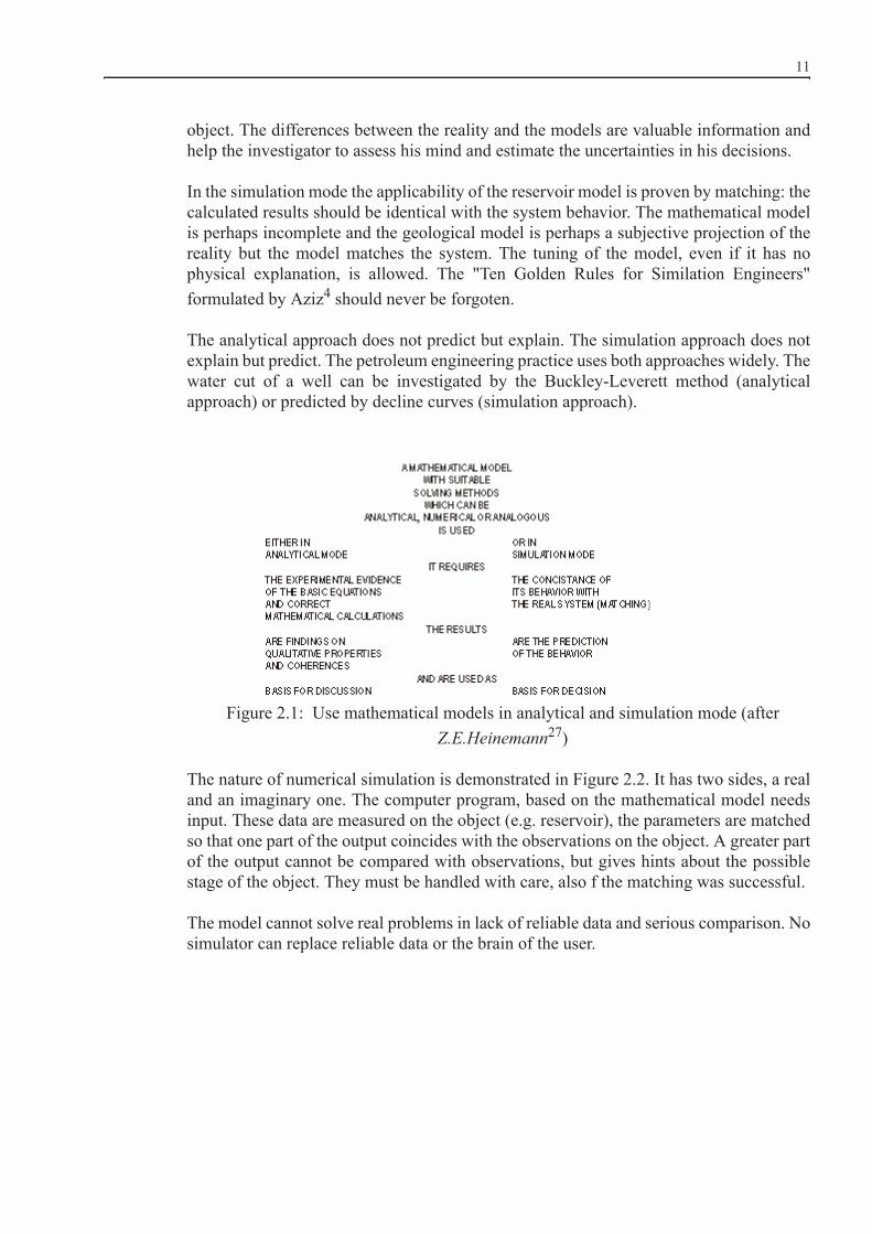
In the simulation mode the applicability of the reservoir model is proven by matching: thecalculated results should be identical with the system behavior. The mathematical modelis perhaps incomplete and the geological model is perhaps a subjective projection of thereality but the model matches the system. The tuning of the model, even if it has nophysical explanation, is allowed. The "Ten Golden Rules for Similation Engineers"formulated by Aziz4 should never be forgoten.
The analytical approach does not predict but explain. The simulation approach does notexplain but predict. The petroleum engineering practice uses both approaches widely. Thewater cut of a well can be investigated by the Buckley-Leverett method (analyticalapproach) or predicted by decline curves (simulation approach).
Figure 2.1: Use mathematical models in analytical and simulation mode (after Z.E.Heinemann27)
The nature of numerical simulation is demonstrated in Figure 2.2. It has two sides, a realand an imaginary one. The computer program, based on the mathematical model needsinput. These data are measured on the object (e.g. reservoir), the parameters are matchedso that one part of the output coincides with the observations on the object. A greater partof the output cannot be compared with observations, but gives hints about the possiblestage of the object. They must be handled with care, also f the matching was successful.
The model cannot solve real problems in lack of reliable data and serious comparison. Nosimulator can replace reliable data or the brain of the user.

12
Figure 2.2: The nature of numerical simulation (after Z.E.Heinemann27)
2.3 History Matching
2.3.1 What is It?
It is not possible to cover all aspects of the HM. It is not even possible to give a summaryof today’s stage of the History Matching Techniques, within the frame of this work.Standard History Matching Techniques are composed of a fixed geological model (StaticModel) with global modifications and local adjustment. The limitations of thismethodology are clear. Local adjustments are not always geologically realistic, staticuncertainties are not taken into account and only a limited number of models are used forprediction.
To be fully understandable this traditional workflow is to generate one dynamic modelbased on the single static reservoir model. This was done by modifying the dynamicmodel until the dynamic model corresponded to the historic field data. This is calledhistory matching. The resulting model could be quite different to the static model whichwas used at the starting point of whole tuning procedure. This traditional workflow isdescribed by the chart displayed in Figure 2.3.

13
Figure 2.3: Standard Simulation Workflow
While the capabilities of geosciences improved onwards to create a very detailed andreliable static model due to improved 3D and cross-well seismic, data integration andstochastic modeling, another approach to reach a history matched dynamic model isfeasible.
This new approach goes away from the task to generate one matched dynamic modelbased on one tuned static model. It shifts towards a fast and reliable verification of thenumerous static models. In principle the task remains the same. This is to get one validhistory matched dynamic model.
The new idea is to find the best fitting realization out of many, equally probable staticmodels resulting from stochastic modeling. This new workflow is outlined in Figure 2.4.
Traditional History Matching WorkflowTraditional History Matching Workflow
StaticGeological
ModelDynamic
Data
DynamicReservoir
Model
History Matching
Loop
MatchedReservoir
Model
StaticGeological
Model
StaticGeological
ModelDynamic
DataDynamic
Data
DynamicReservoir
Model
DynamicReservoir
Model
History Matching
Loop
MatchedReservoir
Model
MatchedReservoir
Model
StaticGeological
Model
MatchedReservoir
Model
Resulting indifferent
StaticGeological
Model
StaticGeological
Model
MatchedReservoir
Model
MatchedReservoir
Model
Resulting indifferent

14
Figure 2.4: New Simulation Workflow
The classical approach in history matching is a step-by-step procedure altering thegeological reservoir model until the output of the reservoir simulator fits to measured fielddata within acceptable limits.
This approach is shown in Figure 2.5. Note that the arrays are oriented from left to right,in principle any parameter may be adjusted.
Normally these parameters include permeabilities, porosities, fault transmissibillities andthrows, aquifer strength, rock compressibility and initial fluid contact depths. Geologicaland petrophysical properties of the productive areas are well known through differentgeophysical and geostatistical methods.
History matching mainly deals with aquifer properties, since only few or even no data areavailable about this part of the reservoir model.
Throughout the process of history matching the aquifer model becomes more and morecomplex. This is done by re-sizing and re-parametrizing the grided aquifer or by changingthe parameters of analytical aquifer models without changing the productive area.
Desired History Matching WorkflowDesired History Matching Workflow
StaticGeological
Model
StaticGeological
Model DynamicData
DynamicData
DynamicReservoir
Model
DynamicReservoir
Model
InnerHM
Loop
MatchedReservoir
Model
MatchedReservoir
Model
StaticGeological
Model
StaticGeological
Model
in identicalResulting
DynamicReservoir
Model
DynamicReservoir
Model
DynamicReservoir
Model
DynamicReservoir
Model
DynamicReservoir
Model
DynamicReservoir
Model
StaticGeological
Model
StaticGeological
Model
StaticGeological
Model
StaticGeological
Model
StaticGeological
Model
StaticGeological
Model
OuterHM
Loop
MatcheddynamicModel
MatcheddynamicModel
If it succeeds

15
Figure 2.5: Validation of a dynamic resevoir model in a conventional approach
2.3.2 Quality of History Match
The results of the well by well HM are the static and dynamic BHP, the cumulative oil,water and gas production and the production rates at the end of the history.
Which items are more important in a given case depends on the quality of the data and ofthe geomodel, on the nature of reservoir, the depletion mechanisms and - very strongly -on the objective of the study.
New HM Workflow New HM Workflow -- Conventional ApproachConventional Approach
StaticGeological
Model DynamicData
DynamicReservoir
Model
InnerHM
Loop
DynamicReservoir
Model
DynamicReservoir
Model
DynamicReservoir
Model
StaticGeological
Model
StaticGeological
Model
StaticGeological
Model
OuterHM
Loop
StaticGeological
Model
StaticGeological
Model DynamicData
DynamicData
DynamicReservoir
Model
DynamicReservoir
Model
InnerHM
Loop
DynamicReservoir
Model
DynamicReservoir
Model
DynamicReservoir
Model
DynamicReservoir
Model
DynamicReservoir
Model
DynamicReservoir
Model
StaticGeological
Model
StaticGeological
Model
StaticGeological
Model
StaticGeological
Model
StaticGeological
Model
StaticGeological
Model
OuterHM
Loop
Field water rate
Field oil rate
Well static pressures
Field water rate
Field oil rate
Well static pressures
Phase rates and reservoir pressures are calculated.
With other words they are theOUTPUT !
OK if the result is comparable with the history otherwise NOT!
16
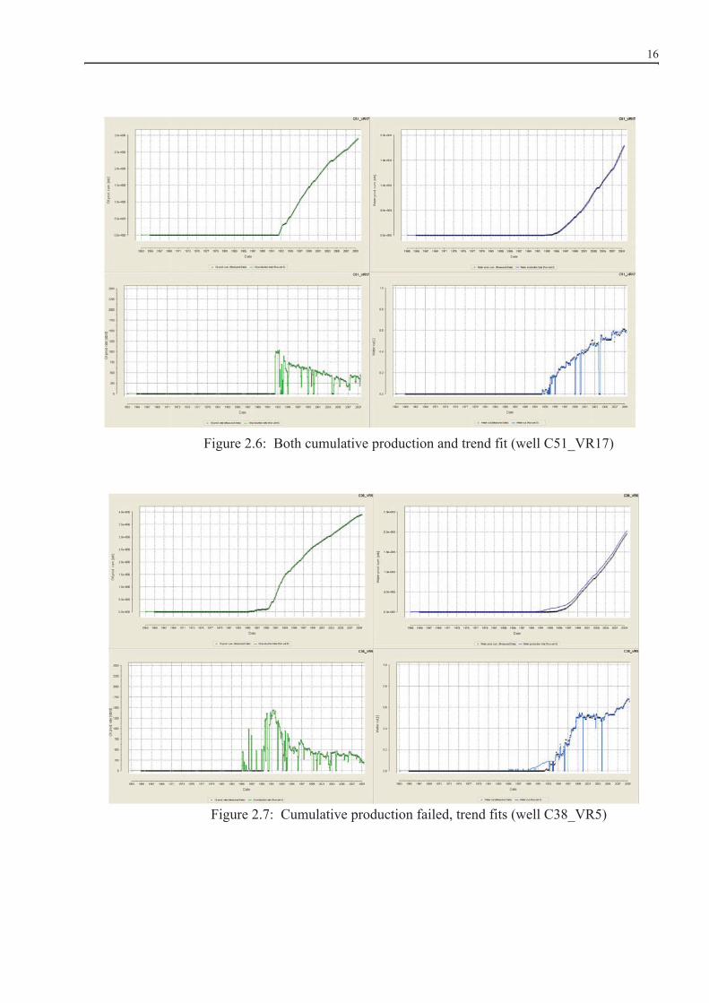
Figure 2.6: Both cumulative production and trend fit (well C51_VR17)
Figure 2.7: Cumulative production failed, trend fits (well C38_VR5)

17
Figure 2.8: Cumulative production fits, trend failed (well C23_VR)
Figure 2.9: History match of the well failed (well C35_VR4)
Figure 2.6 to Figure 2.9 show wells "history matched" on different level. The figures aretaken from a real project but serve here for demostration only.

18
Figure 2.6 shows an optimally matched well. The cumulative oil and water production isreproduced for the entire production period and the slope of the curves in the last years fitto the observations. Only the differences in the production rates are apparent. Thehistorical data are given on monthly basis; the simulator uses the quarterly averages insake of more flexibility in time step regulation and better numerical stability. If most ofthe wells are matched with this quality then two requirements of highest importance aresatisfied:
• The correct amount of oil and water are located at every well drainage area all thetime. Therefore it can be assumed that the distribution of the phases in the reservoir ismodelled correctly and the place of the remaining oil is determined credibly. Themodel reproduces today’s well productivity. Therefore the model can be used topredict the well and field performances.
Figure 2.7 and Figure 2.8 show two weakly matched cases. In the first case the cumulativeproduction fits, but the match of today’s trend failed. The second case is the opposite. Thewell in Figure 2.9 failed completely.
2.3.3 Automated and Computer Assisted History Matching
Basically history matching is done by a trial and error process that is mainly influencedby the experience, intuition and judgement of the simulation engineer, it can be a verytime consuming and costly step in a standard simulation workflow. A good description oftraditional history matching methods can be found in Williams et al.65. To improve theeffectiveness of history matching and to automate, and therefore, shorten this costly stepwas the focus of the last years. The goal was and still is to find ways to an automatedhistory matching by implementing different algorithms to find the minimum of a so calledobjective function. Such an objective function quantifies the differences betweenobserved and simulated values.
One way of optimizing history matching is the use of the gradient method. Such a methodwas developed by Anterion et al.3. This method requires the derivatives of the componentsof the objective function with respect to the history matching parameters. This means thatthe reservoir engineer is able to test his ideas by making repeated simulation runs withaltered parameters. If an improved match is achieved, he can guess - by applying thegradient method - how much the altered parameter have to be changed to get a matchedmodel or matched part of the model. Tan and Kalogerakis59,60 used this method to solvea model problem. Bissell et al.7,8 applied it to real field cases.
A hybrid method where gradient optimization is combined with a direct search methodwas developed by Leitato et al.37. Additionally parallel computing was used to speed upthe procedure. Schiozer56 worked with an similar approach. The main achievements ofboth developments were the gained speed-up factors by using parallel computing.
19
Regarding effectiveness of finding and correctness of the parameters their work can becompared to other methods.
The gradient method has some shortcomings such as distortion of variogramscharacterizing the spatial distribution of two parameters like porosity and permeability ifthey are simultaneously updated. To overcome some of them, new ideas wereintorduced.These were the combination of the gradient method with geostatisticalparameterization techniques such as the pilot point method of Bissell et al.7 or the gradualmethod of Roggero et al.53.
Using genetic algorithms40,49,52, simulated annealing techniques39, neural networks orresponse surfaces17 are other recent approaches how to deal with the minimizationproblem of history matching.
Until now, none of the techniques described above has gained a wide acceptance as auseful tool for history matching. According to MacMillan et al.39 this results from the factthat all these methods assume that all the matching parameters have been determined andthat the model is fixed. They further assume that the only thing is to adjust thoseparameters to get a matched model. As a way out MacMillan et al. developed tools toassist the simulation engineer to find the correct parameters and their neededmodifications.
Emmanuel et al.18 defined the term assisted history matching as using algorithmictechniques to assist the process of traditional history matching. They used the flowpath of3D streamlines to assist the process of altering reservoir parameters. Le Ravalec-Duoinand Fenwick38 also use the concept of streamlines. They combined it with geostatisticaltools and the gradient method.
Also Sarma at al.54 introduced a new approach to automatic History Matching usingKernel PCA; in this way they apply a new parameterization referred to as a kernelprincipal component analysis (kernel PCA or KPCA) to model permeability fieldscharacterized by multipoint geostatistics.
Schulze-Riegert and Shawket Ghedan57 presented in the 9th international forum onreservoir simulation a Modern Technique for History Matching, dealing withuncertainties in reservoir data. It is not within the scope of this thesis to give a historicaloverview or to discuss all advantages and limitations of alternative techniques but anextended reference list is added for this purpose.
TPPM is not comparable with all those methods from the simple reason that no reservoirparameters will be modified but the well position and perforation properties. From thisrespect TPPM opens a new classe of computer assested history matching methods.

20
2.4 Aquifer Models
2.4.1 Introduction and background information to Aquifer Modeling
Today’s reservoir characterization, modeling, advanced well logging and interpretationmethods, as well as modern production surveying and monitoring systems deliver moreand more detailed information about the reservoir. The step-up in quality and quantity ofdata generally reduces the attempt of the date of the interview process, but all of thesemethods usually are not applied to the aquifer of the reservoir. As the aquifer is frequentlynot covered by modern reservoir modeling techniques, great uncertainty regarding thecharacterization and parameters are the result.
A large number of oil and gas reservoirs have an associated aquifer, that provides themwith pressure support. The reservoir and the aquifer form a hydraulic system and apressure decline accompanying production results in water encroachment into thesereservoirs. The importance of this water movement derives from the significantdependence of production rate upon reservoir pressure, in turn, upon water encroachment.For this reason a successful simulation study is only possible if the complete system,reservoir and aquifer, is taken into consideration and not only the hydrocarbon bearingpart.
Fundamentally there are two possibilities to model the water inflow into a reservoir:
1. Representing the aquifer by a grid model2. Using analytical models
According to Heinemann22 a reservoir model can be built from two fundamentallydifferent domains. One is the reservoir itself, the other one is the connected outer aquifer.The grids for these domains are constructed independently but are combined to one fullfield project. This results in an Aquifer Grid and in a Productive Area grid. InHeinemann’s concept "reservoir" and productive area (PA) have slightly differentmeanings, because the PA normally covers a part of the water bearing formations too,called inner aquifer. As already mentioned the PA and the Aquifer are modeled byindependent grids, which can be linked to each other, or with other words, they can bemerged into one single grid model.
Most of the commercial modeling packages do not make this splitting. The whole gridwill be constructed in one step. In such a case the PA grid can be created by deactivatingthe aquifer grid blocks and the aquifer grid by deactivating the reservoir grid blocks.
This chapter deals with both kinds of aquifer models. The splitting of the model in PA andAquifer grid has the advantage that for a given PA, both a gridded as well as an analyticalaquifer model, can be used. The combination of the two methods provides considerableadvantages for the history matching especially aquifer matching, as will be shown

21
throughout this thesis. In this chapter the basic methods will be introduced. It will beshown that the two methods, using them in the right way, provide comparable results.
2.4.2 Gridded Aquifer Models
While the geological and petrophysical properties of the productive areas are known at thebeginning of a simulation project, the aquifer is usually unknown. The size, the porosity,the permeability and their distributions around the productive area will be determined bymatching reservoir pressure. In lack of other possibility the aquifer is regarding isotropicin areal extension, i.e.: the permeability does not depend on the direction. The HistoryMatch is a step-by-step procedure in which the aquifer model becomes more and morecomplex by re-sizing and re-parametrization of the aquifer without changing theproductive area, The aquifer grid is constructed from the global mesh outside the PA, (fullexplanation in Appendix 5)
.Figure 2.10: Simulation model with gridded aquifer (after Heinemann22)
2.4.3 Analytical Aquifer Modeling
2.4.3.1 Aquifer Models
Because of the recognition that the reservoir and the aquifer form a hydrodynamic system,

22
it became necessary to find methods to relate aquifer behavior and reservoir response. Thefirst dependencies have been developed in the 1930’s by using material balanceformulations.
The dominance of material balance calculations for determining aquifer behavior becameless in the 1960’s when numerical reservoir simulation became more and more usable.These achievements lead to an integration of water influx calculations and as a result moresophisticated techniques were found. Outside numerical reservoir simulation most waterinflux calculations are based on aquifer behavior models. Theses models describe how theaquifer responds to changes in the reservoir. This response is expressed as a water influxrate. Assuming an aquifer behavior model with an analytical solution is common practice.
To establish aquifer models two different approaches can be used, the first is to establisha model based on idealized mathematical models, these models are idealized so far as theyassume homogeneous reservoir properties like uniform porosity, permeability, etc, butthese models are also idealized in another way, concerning reservoir and flow geometry.This idealization is expressed either by radial or linear models.
The second approach to develop aquifer behavior models is based on a direct integrationof field data, this leads to models without idealized assumptions concerninghomogeneities and geometries. In 1936 Schilthuis55 published a model according to thefirst approach described above.
Schilthuis developed a model for steady-state water influx behavior, this means that thismodel is applicable if the aquifer is of such an extent that water influx to the reservoir doesnot alter the aquifer pressure observably, this would correspond to an aquifer of infinitedimensions. Since the size of an aquifer is usually limited this method is only applicablein a few cases.
To describe aquifers that change their pressure over time it became necessary to developaquifer behavior models that take into consideration this non steady state water influx.Hurst and VanEverdingen62 in 1943 and Carslaw and Jaeger11 in 1959 have developedsuch models based on the solution of the differential diffusitivity equation. The solutionpresented by Carslaw and Jaeger is valid for linear aquifers whereas the solution of Hurstand VanEverdingen63 is valid for radial symmetrical geometries. Both methods have twodisadvantages in common. The first is that they do not support an analytical solution tosolve water influx problems of aquifers with arbitrary shape. The second is that bothmethods use the principle of superposition to allow a time dependent reservoir boundarypressure. Therefore, their methods result in a lengthly and tedious calculation forincreasing time steps.
In 1987 Vogt and Wang64 published an improvement to the model of Hurst andVanEverdingen63. This was done by substituting the stepwise constant reservoir-aquiferboundary pressure - used by Hurst and VanEverdingen63 to apply the principle ofsuperposition - by a piecewise linear one. Besides gaining better results if the pressurechanges quickly especially at early times another advantages is inherent to the Hurst and

23
VanEverdingen63 method. This is that the piece-wise linear approximation is moreconvenient for computer programming.
To avoid the unpleasantness related to the principle of superposition Carter and Tracy10
proposed a method in 1960 to solve water influx calculations for transient circular aquifermodels analytically based on the solution of Hurst and VanEverdingen. They assumedconstant water influx for any given time step. Since this is not strictly valid, their methodis not as accurate as the one by Hurst and VanEverdingen.
All aquifer behavior models for non steady-state water influx mentioned above have incommon that they are restricted to regular shaped reservoir and aquifer boundaries. Forcomplex water influx geometries Numbere48 developed a method in 1989. This methodallows to calculate a dimensionless influx function for complicated geometries ofreservoirs as well as aquifers. Katz et al.35 as well as Carter and Tracy10 have chosen thesame approach for other reservoir studies. They showed with their publications thevalidity and utility of the method of Numbere48 but also extended this method toadditional reservoir-aquifer geometries resulting in additional tables.
In 1969 Fetkovich19 published a different approach of how to deal with the water influxproblem without knowing the reservoir aquifer geometry. The developed model is largelyempirical and assumes a pseudo steady-state flow behavior. This means a finite aquiferwith a short transient period. Because of its empirical character no guidelines when thismodel is applicable can be given.
The second approach to establish aquifer behavior models is to use direct field data.Therefore, such models are only valid for a particular aquifer-reservoir combination.Using this approach, an influence function F(t) is established which links watermovement uniquely to a reservoir aquifer combination. Since this influence function isbased on direct field data a consideration of heterogeneity and geometry can take place.Hutchinson and Sikora34 and Katz, Tek and Jones35 dealt with aquifer influencefunctions. They encountered difficulties if the field data showed inaccuracies.
A general theory for aquifer behavior was developed by Coats, Rapaport, McCord andDrews12 in 1964. Their theory was based on a general aquifer that was heterogeneous,arbitrarily shaped and that had rock properties such as permeability, porosity and totalcompressibility that were independent of pressure. They showed that the general solutionto this problem can be described using infinite series. Using infinite series the three basicflow behaviors of aquifers (steady-state, none steady-state and pseudo steady-state) areonly special cases of their general formulation. The method of Coats et al.12 was extendedand improved later by various studies.
Still, all these models and improvements share one general drawback. They are dependenton an estimate for the water influx to match the aquifer influence function.

24
2.4.3.2 Inflow into the Artificial Boundaries
Fluid flow processes in reservoirs are simulated by using discretized forms of partialdifferential equations. They result from the combination of balance equations describingthe conservation of mass and Darcy’s law. These equations linking fluid flow rate,pressure, reservoir and fluid properties are of mixed hyperbolic-parabolic type. Alongwith appropriate constraints, constitutive relations, boundary and initial conditions thediscretized forms of the partial differential equations can be solved numerically.
Amado et al.2 derived a general implicit mole balance equation using the Control VolumeFinite Difference (CVFD) discretization scheme given in Equation 2.1. This formulationconsists of the flow or convection term on the left-hand side and the accumulation termon the right-hand side only. The source/sink term, expressed by Equation 2.2 can be addedto the left hand side whenever necessary.
(2.1)
, (2.2)
where
tij blockpair transmissibility [Darcy.m]xpc mole fraction of component c in phase p [-]lp mobility of the phase p [cp-1]Dp specific mole density [kmol/m3]n number of time steps [-]qp source/sink term for phase p [kmol/day]Dt time step [day]Vi volume of grid block I [m3]f porosity [-]Sp phase saturation [-]
and the indices limits are
P number of phasesC number of componentsN number of neighboring grid points for point i.
Various types of boundary conditions can be defined. Boundaries used in reservoirsimulation can be classified generally either as inner or outer boundaries. Outer
ij pDpxpc ijn 1+
pj pi– n 1+
p 1=
P
j 1=
NVi
t----- t SpDpxpc
p 1=
P
i
=
qpxpc In 1+
p 1=
P

25
boundaries are the top and the bottom of the domain, as well as the outer delimitation lines(surfaces). Examples for inner boundaries are discontinuity lines (surfaces) such as faults.The major difference between outer and inner boundaries is, while the outer boundary hasone side only, the inner boundary separates or connects two different domains (orsubdomains).
For outer boundaries two types of conditions can be applied. Boundary conditions ofDirichlet type (Equation 2.3) define the potential at the boundary and boundary conditionsof von Neumann type (Equation 2.4) define the flow rate across it.
(2.3)
(2.4)
If the boundary is sealing (no-flow boundary) then is valid.
Inner boundaries are characterized by the flux continuity condition given by Equation 2.5.
, (2.5)
where
permeability tensor [Darcy]normal unit vector [m]
t time [s]filtration velocity [m/s]
F phase potential [Pa]l phase mobility [1/Pas]p phaseG boundary
and the indices ir and il denote the right- and left-hand sides of the discontinuity surface.
In work of Pichlbauer51 the concept of Artificial Boundaries (AB) is introduced.Artificial boundaries can, but do not have to, have something in common with naturalboundaries, defined above. From a mathematical aspect they are not boundaries, becauseno boundary conditions will be applied to them. An Artificial Boundary is built by anarbitrary row of blocks, representing a line or a surface anywhere in the grid model.
Artificial Boundaries will be used as tools to enhance the modeling process, mostly theHistory Matching process. For an already existing grid model it is possible to define oneor more of such boundaries. This kind of "boundaries" is characterized by supplementarysource/sink terms, which means, that fluid can be injected in, or produced from theseblocks under defined conditions. These source/sink terms can be cancelled anytime. Thismeans that the former boundary blocks become “normal” blocks again. With other words,
t=
up t pk pn–=
up 0=
kir irni kil ilni=
kn
u
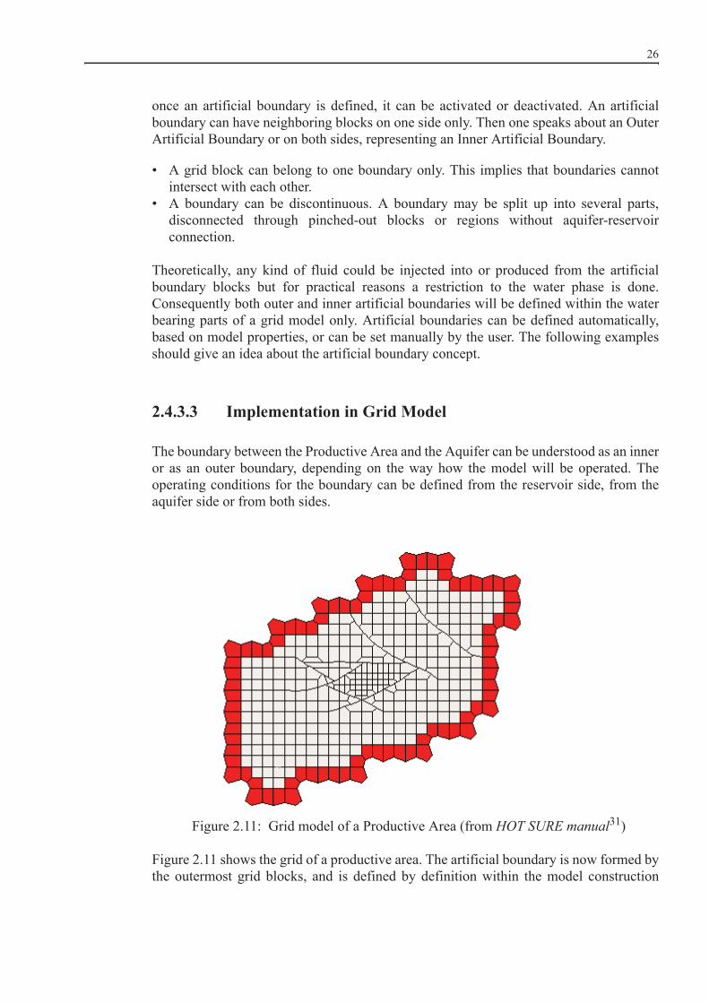
26
once an artificial boundary is defined, it can be activated or deactivated. An artificialboundary can have neighboring blocks on one side only. Then one speaks about an OuterArtificial Boundary or on both sides, representing an Inner Artificial Boundary.
• A grid block can belong to one boundary only. This implies that boundaries cannotintersect with each other.
• A boundary can be discontinuous. A boundary may be split up into several parts,disconnected through pinched-out blocks or regions without aquifer-reservoirconnection.
Theoretically, any kind of fluid could be injected into or produced from the artificialboundary blocks but for practical reasons a restriction to the water phase is done.Consequently both outer and inner artificial boundaries will be defined within the waterbearing parts of a grid model only. Artificial boundaries can be defined automatically,based on model properties, or can be set manually by the user. The following examplesshould give an idea about the artificial boundary concept.
2.4.3.3 Implementation in Grid Model
The boundary between the Productive Area and the Aquifer can be understood as an inneror as an outer boundary, depending on the way how the model will be operated. Theoperating conditions for the boundary can be defined from the reservoir side, from theaquifer side or from both sides.
Figure 2.11: Grid model of a Productive Area (from HOT SURE manual31)
Figure 2.11 shows the grid of a productive area. The artificial boundary is now formed bythe outermost grid blocks, and is defined by definition within the model construction

27
process. This boundary connects the PA grid to the aquifer grid, or the boundary blocksserve as entry points for the water influx, calculated from an analytical aquifer model. Inthe first case the artificial boundary is an inner boundary, in the second case an outerboundary.
The boundary does not have to be continuous for the whole PA. It is possible to split it upinto more segments. The splitting has the advantage that different conditions can bedefined for each part of the reservoir. In Figure 2.12. the gridded reservoir area issurrounded by three outer boundaries. Naturally it is possible that a grid model has aboundary on one side only.
Figure 2.12: Segmented Outer Boundaries and appropriate Target Areas (from Mittermeir44)
In Figure 2.12 the white boundary belongs to the cyan target, the red boundary to the lightblue target area and the dark blue boundary belongs to the light brown target area. Thecenter (displayed in orange) area is separated by sealing faults from the rest of thereservoir.
2.4.3.4 Average Boundary Pressure
For most of the applications the average pressure of the boundary must be known. It canbe calculated as a weighted average of the boundary block pressures:

28
, (2.6)
where
j index number of the boundary blocks j = 1,..., mwj weighting factor for the boundary block jpj pressure of the boundary block jpr average pressure of the boundary
Weighting factor wj can be either the transmissibility to the connected region or the porevolume of the boundary blocks.
2.4.3.5 Distribution of a Given Rate between the Outer BoundaryBlocks
Except for the case of a constant pressure boundary, the total water rate through theboundary qwn is determined, which must be distributed among the boundary blocks. Thegoal is that the individual block pressures converge to the average boundary pressure pr.Therefore the overall rate will be distributed based on a kind of injectivity index:
if , else (2.7)
where j is a non boundary neighbor of the boundary block i and TRij is the transmissibilityfor the block pair i and j. If the block i has more than one neighbor, than the injectivityindices will be summed up. If a block j is neighbor to more than one boundary block thanthe injectivity index has to be reduced accordingly.
Let qwn be the overall boundary rate during a time step Dtn, then the rate injected into theboundary block i is:
(2.8)
pr
pj jj 1=
m
jj 1=
m---------------------=
Ji ij pr pj–= pr pj 0– Ji 0=
qwi nJi
Jii
----------- qwn=
29
2.5 Target Pressure Method
2.5.1 Previous Works
The first step in every History Matching is to determine the objective functions. They are,among others, the well bottom hole pressures, water cuts, GOR etc., but the primaryobjective must be to match the average reservoir pressure and the pressure for givenvolume regions. If these pressures do not fit to the measured ones, then there is no chanceto achieve a well by well match with the used reservoir model. For a volume region theaverage pressure is usually given as a pore volume weighted average or as a hydrocarbonweighted average which will be calculated from the regular pressure surveys.
The region pressures depend on the production and on the water influx from the aquifer.The concept of Artificial Boundaries allows to match the historical average pressuresdirectly, without the usual trial and error procedure. The idea is called Target PressureMethod (TPM). The principle and the corresponding work flow will be explained for themost simple case.
Consider one Productive Area with one Artificial Boundary around it, as shown in Figure2.11. The target volume region is now the whole grid without the boundary blocks. Notethat the blocks of the boundary are one phase water blocks, with constant salinity and thatno grid describing an aquifer is present.
For the Target Pressure Method the average pressure and the overall compressibility ofthe volume region must be calculated at the end of every time step j. The average pressureis:
, (2.9)
where the weighting factor, w, is the total or the hydrocarbon pore volume of block i. InEquation 2.9 pi is the actual calculated pressure of the blocks and m is the number ofblocks. The overall compressibility of a block i is
. (2.10)
The total compressibility of the volume region is the sum of the block compressibilities:
pjav
i pii 1=
m
ii 1=
m-------------------------=
Ci Vpi c Soco Sgcg Swcw+++ i=

30
. (2.11)
In this equations
m is the number of blocks in the target areaVpi is the pore volume of block i [m3]
is the pore compressibility factor of one single block [bar-1]Sp is the phase saturation (p = o,g,w) [-]cp phase compressibility factor (p = o,g,w) [bar-1]Ct total compressibility [m3/bar]
Let qwn be the overall boundary rate during a time step Dtn, then the rate injected into theboundary block i is:
. (2.12)
The rate must be defined for every time step individually. This procedure includes thefollowing steps:
1. Predict the calculated pressure changes for the following time step, , based onthe pressure decline rates of the previous two time steps.
2. Determine the difference between the predicted and the target pressure for this timepoint: .
3. Determine the volume of water which should be added to the target volume regionto hit the target pressure. This can be calculated based on the overall compressibilitygiven by Eq. 2.11:
. (2.13)
4. The injection rate for the Artificial Boundary during the time step is:
, (2.14)
which will be distributed among the boundary blocks according to Equation 2.8.The injection rate for the first time step is always zero.
Mittermeir44 published an example to demonstrate the properties of the TPM. Figure 2.13shows the pressure propagation of the reservoir and Figure 2.14 shows the attainedboundary pressure propagation with the associated water injection rates.
Ct Cii 1=
m
=
c
qwi nJi
Jii
----------- qwn=
tn
p
W Ct p=
tn
qwn W tn=

31
Figure 2.13: Comparison of the result of the TPM calculation with the measured data (from Mittermeir44)
Figure 2.14: Boundary pressure and injected water into the artificial outer boundary (from Mittermeir44)
As can be seen in Figure 2.13 the average reservoir pressure was matched very accuratelyin one single simulation run. The injection rate that is plotted in Figure 2.14 as a functionof time oscillates strongly. This is caused by the explicit implementation of the TPM. Thismeans that the water injection is calculated at the beginning of every time step. As aconsequence these oscillations can be found in the boundary pressure and the averagepressure of the productive area also, although they are smoothed out in the averagepressure of the target area. After Mittermeir45 these oscillations could be reduced by using
180
200
220
240
260
280
0 365 730 1095 1460 1825 2190 2555 2920 3285 3650
Time [days]
Avg
. HC
wei
ghte
d R
eser
voir
Pres
sure
[bar
]
Measured - Gridded Aquifer Simulated - Target Pressure Method
180
200
220
240
260
280
0 365 730 1095 1460 1825 2190 2555 2920 3285 3650
Time [days]
Bou
ndar
y Pr
essu
re [b
ar]
0
5000
10000
15000
20000
25000
Inje
ctio
n R
ate
[sm
³/day
]
Boundary Pressure W aterinjection rate
32
smaller time steps, but since the reservoir pressure is only influenced very little, theseoscillations have no practical importance. The author found, in connection with his fieldproject Lower-GIR1, that this statement in not generally valid. His suspicion wasconfirmed by practical application of TPPM to the field Augila and Alborz (privatecommunication Harrer20)
It should be emphasized that the target pressure method is applicable to reproduce thehistory but no prediction can be performed in this way. The next step must be to find anaquifer model which provides the necessary water influx over the whole time period basedon the calculated boundary pressure of the TPM. Such an aquifer representation can beeither an analytical aquifer model or a gridded aquifer. Both will smooth out the waterinjection rate and the boundary pressure efficiently. The suggested workflow byMittermeir44 is:
1. Identify the optimal analytical aquifer models and their parameters.2. Calculate the history with those analytical aquifer models to verify the results of the
TPM run.3. Calculate the extent and permeability of a gridded aquifer.4. Fine tuning of the History Match using the gridded aquifer model.5. Perform the prediction runs.
2.5.2 Identification of the Optimal Analytical Aquifer Model
Besides supporting the reservoir from the first moment of the history matching periodwith the correct water influx, the TPM produces another very important and valuableoutput. This output is stated in form of the best fitting analytical aquifer parameters. Asresults of the TPM run, the boundary pressure and the cumulative water inflow, W, areavailable as a function of time for the whole period of past production. This is analogousto the results of a material balance calculation, and can be used in a similar manner todetermine the parameters of the best fitting analytical aquifer model. For this, thefollowing error function should be minimized:
(2.15)
where n is the number of time steps, We is the result from one of the models described inSection 3.3. wj = tj/tn is a usual weighing factor. This means that the differences in waterinflux at a later time have more weight as the earlier ones. Different analytical aquiferformulations require a different number of parameters describing it. For the Schilthuismodel one (C), for the Fetkovich19 model two (Jw,Wei), and for the vanEverdingen-Hurst63, Vogt-Wang64 and Carter-Tracy10 models three parameters (rDe,
E j W tj We tDj– 2
j 1=
n
=

33
and C) will be determined. For all models also the standard deviation, s, will be calculated,showing which model type is the best one. Using this best fitting aquifer model, the runcan be repeated and proven if the historical pressure can be satisfactory reproduced or not.If this is possible, it can be expected that the analytical model is suitable to provide therequired water influx for prediction runs. This is especially the case if the aquifer does notmanifest complicated or irregular behaviors.
For all analytical aquifer models mentioned above, the parameter pairs or triplets fittingbest are determined using a generic algorithm. Detailed description of this procedure isgiven by Pichlbauer51, Mittermeir44 and in PRS Technical Description29.
2.5.3 Application of TPM to TPPM
2.5.3.1 Experiences
As already mentioned the Target Pressure and Phase Method is an extension of the TargetPressure Method. Theoretically all three aquifer types could be applied to TPPM. PRSoffers all of them, ECLIPSE only Fetkovich19 and Carter-Tracy10. The Vogt-Wang64
model which is in fact the same as the Hurst-van Everdingen63 model, is not available inECLIPSE. The Carter-Tracy model is an approach to the Hurst-Everdingen model withthe apparent advantage that it is not necessary to store the boundary pressures for allprevious time steps. For this reason the Carter-Tracy model become popular in the earlytime simulation software (Three-Three, ...., but also ECLIPSE). Numerical experimentsshowed that the results from PRS and ECLIPSE differ up to 20%, which is not a problemusing both simulators independently because the parameters will be tuned during the HManyway. For TPPM this discrepancy is unfortunate, It deteriorates the compatibility of thetwo simulators. How the Carter-Tracy model is implemented in ECLIPSE is not knownand the code is not accessible for the author. No insufficiency or bug could be identifiedin PRS and so there is nor reason to doubt its correctness. In this situation the Fetkovichmodel is the only one usable today for TPPM.
2.5.3.2 Improvements
It can be checked easily, how good the aquifer modeling works. The target pressure runmust be repeated with the analytical aquifer model, using the parameters determinedautomatically by PRS. The run can be repeated with ECLIPSE too, checking thecompatibility also. Simple small (academic) models gave mostly satisfactory results.Experience with the large full field cases as Upper-Gir, Augila and Amal (mentiond inSection 2.5.3.1) showed that some improvement would be advantageous. Two possiblediscrepances between the ptarget and fetkov approach would be presumed and eliminatedin PRS:

34
1. Using ptarget option the water influx (injection in boundary) is calculated for apredicted average region pressure after a given time interval. The fetkov optioncalculates the water influx based on the actual average boundary pressure. Theauthor introduced an alternative option, govered by keyword, considering theaverage region pressure instead of the average boundary pressure.
2. ptarget handle the boundary block pressures impicit the fetkov expicit. The authorchanged the second one to an implicit formulation.
The following example shows that this heuristic approach could be regarded as asuccessful step. A deeper investigation and scientific prove of this question is beyond theobjectives of this work.
2.5.3.3 Fetkov Test Model
While conducting this thesis work it was discovered that the two simulation packages inuse, PRS and ECLIPSE, give different results when an analytical aquifer model ofFetkovich type was used. Depending on the complexity - in terms of phases (oil, water,free gas), number of blocks, extend of the boundary, etc. - the differences could beregarded either as minor or severe. Further it was discovered that tuning the parametersof the Fetkovich model (maximum enroachable water and aquifer productivity index)would lead to satisfactory results. No general rules for tuning could be determined.Consequently this tedious work had to be done in trial and error process for every modelsetup individually. Naturally this is not a satisfactory situation.
In order to be able to investigate the differences between the PRS and ECLIPSE Fetkovichaquifer model implementation, it was decided to create a simple model. One of theobjectives during model design was that this model could be also calculated manually bya simple material balance calculation. Therefore it was decided to create a onedimensional (1D), horizontal, one phase (water) model with one water producing well anda single boundary block. A cross section of this model can be found in Figure 2.15.
Figure 2.15: : Cross-section view of Fetkov Test Model showing well position and boundary location (exaggeration = 50).

35
The entire model consists of 100 blocks. Each of these blocks is, equally shaped withequal dimensions and properties (e.g. porosity, permeability, etc.). Due to the horizontalcharacter of the model all blocks have the same pressure after initialization.
The model was operated for a period of 10 years. During the first 5 years the waterproducer was operated at a constant water production rate of 50m³/day. During this periodthe average pressure of the model decreased leading to a water encroachment from theanalytical aquifer. After this withdraw period the water producer was shut in and themodel was calculated for some other 5 years. Due to the pressure gradient in the model(shown in Figure 2.16) created by the water withdrawal, water encroachment from theanalytical aquifer continued until the average pressure of the model and the aquiferpressure became equal. This is documented e.g. in Figure 2.20.
Figure 2.16: : Cross-section view of Fetkov Test Model showing pressure gradient between water producer and analytical aquifer at 1988/01/01 (exaggeration = 50).
The above mentioned setup was run with PRS and ECL with a time step length of 31 days.The entire input was the same. The input parameters of the aquifer model were convertedfrom ECLIPSE (which is regarded as the reference for this test model) to PRS as shownbelow.
# B O U N D A R Y - D E F I N I T I O N S#----------------------------------------#ECL input is the following:#---------------------------# Datum depth : 1000 [m]# Initial aquifer pressure at datum : 110 [bar]# Inital water volume in the aquifer: 4E+10 [sm3]# Total (rock+wat)compressibility : 10.35e-005 [1/bar]# Aquifer productivity index : 100 [sm3/(bar.day)]# --------------------------------------------------------------#PRS input is the following including detailed conversion steps.#--------------------------------------------------------------# Wei = ct*W*pi# Wei = 10.35e-005 [1/bar] * 4E+10 [sm3] * 110 [bar]# Wei = 4.554000E+08 [sm3]# BOUNDARY Bound1 Fetkov AQUIWEI 4.554000E+08 AQUIJW 100.0

36
Figure 2.17 shows a comparison of average reservoir pressure calculated by PRS (shownin green) and ECLIPSE (shown in blue). Both simulators were operated at a time steplength of 31 days. The ECLIPSE result clearly shows the two periods (water withdrawaland pressure buildup) and a smooth pressure propagation. Contrary the PRS results showsa very unsteady, zig-zag like pressure propagation. The PRS run was repeated with a timestep length of 1 day. For this small timestep length which is not applicable for full fieldruns also PRS calculated a smooth pressure propagation. This is shown in Figure 2.18.Figure 2.19 displays the cumulative water influx across the boundary/from the analyticalaquifer into the model area. This plot clearly shows an uneven water encroachment for thePRS run with 31 days time step length and an even water encroachment for the PRS runwith 1 day time step length and the ECLIPSE run with 31 days time step length. It shouldbe noted that the cumulative influx and the final pressure are equal for all threeinvestigated scenarios.
Combining the findings of Figure 2.17, Figure 2.18 and Figure 2.19 following conclusioncan be drawn. The uneven water influx calculated by PRS based on a time step length of31 days leads to high pressure (average model and BHP pressure of the water producer)fluctuations. For such a time step length PRS overestimates the required water influx rate,leading to a pressure increase in the model, which hamper further water encroachmentuntil the pressure has declined again.
This observation can be easily explained by the nature of how the analytical aquifermodels are implemented in PRS. PRS treats the analytical aquifers explicitly. This meansthat at the current time step the water influx for the next time step is already estimated.The longer the chosen time step length, the more likely this estimation deviates from theactually required water influx rate.
In order to resolve this problem, implementation of the PRS Fetkovich analytical aquiferwas improved in a way that the calculation is treated now implicitly. The success of thisimprovement is shown in Figure 2.20.

37
Figure 2.17: Comparison of average reservoir pressure calculated with ECLIPSE and PRS (before improvement) at a time step length of DT = 31 days.
Figure 2.18: Comparison of average reservoir pressure calculated with ECLIPSE and PRS (before improvement) at a time step length of DT = 1 days.
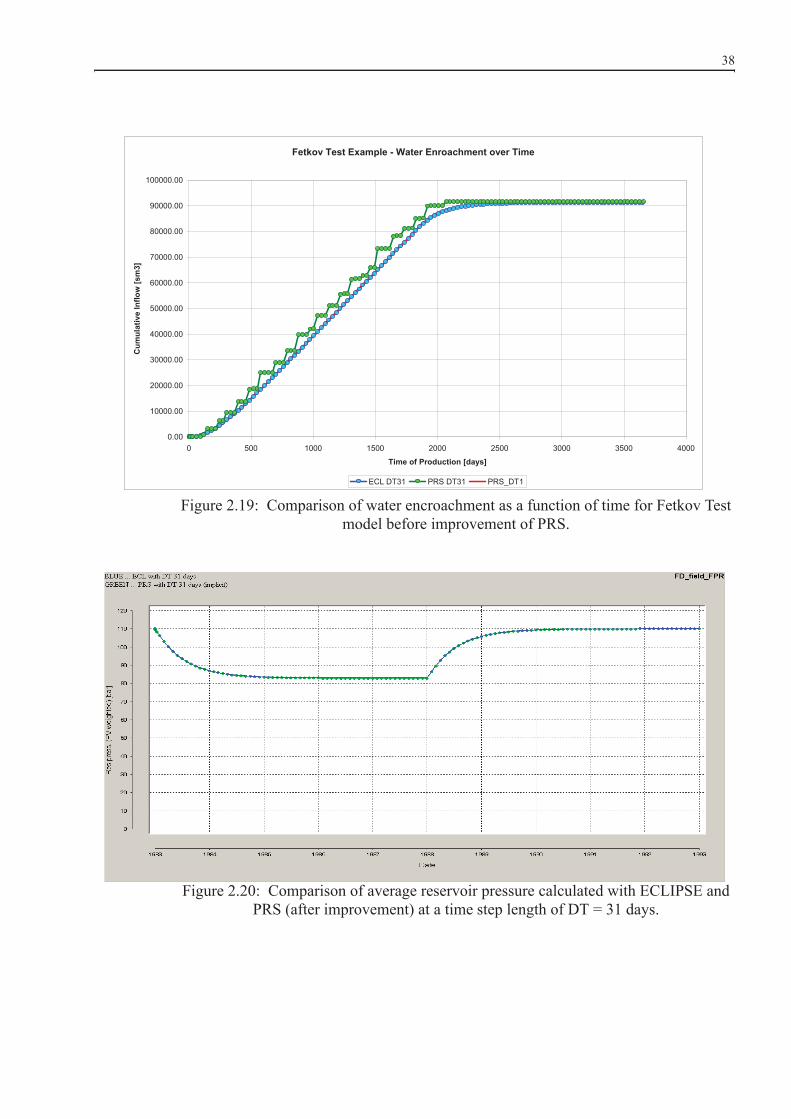
38
Figure 2.19: Comparison of water encroachment as a function of time for Fetkov Test model before improvement of PRS.
Figure 2.20: Comparison of average reservoir pressure calculated with ECLIPSE and PRS (after improvement) at a time step length of DT = 31 days.
Fetkov Test Example - Water Enroachment over Time
0.00
10000.00
20000.00
30000.00
40000.00
50000.00
60000.00
70000.00
80000.00
90000.00
100000.00
0 500 1000 1500 2000 2500 3000 3500 4000
Time of Production [days]
Cum
ulat
ive
Inflo
w [s
m3]
ECL DT31 PRS DT31 PRS_DT1

39
Chapter 3
Target Pressure and Phase Method
3.1 Definition of TPPM
In conventional history matching (HM) process the outputs of the dynamic model werethe pressures and the production rates. They are compared and if they more or less fit tothe historical data then the matching was successful. This process is described anddisplayed on the Figure 2.3 and Figure 2.4. Pichelbauer, Mittermeir andHeinemann51,42,44 introduced the Target Pressure Method (TPM) which made the HMprocess more efficient. The area pressures were defined as input and the boundariesprovide the water inflow (sometimes outflow) following closely the pressures as shownin Figure 3.1. At the end of every run the optimal analytical aquifers were identify andtheir parameters determined. The weekness of the method is that the wells are not able toproduce the assigned oil or gas rates with the meassured GOR and water cut or the wellswere constraint by minimum bottom hole pressure before the end of the HM. To decide ifa given geological realisation is correct or not still needed a time consuming inneriteration as displayed in Figure 2.4.
The author suggested to extend the concept. The basic idea was to define beside the areapressures (Figure 3.1) also the oil, water and gas production rates (Figure 3.2) as targetsand give them as input, also extend the the Target pressure Method (TPM) to a TargetPressure and Phase Method (TPPM). Between the conventional approach in Figure 2.5and the TPPM in Figure 3.3 is the difference that the arrows have the opposite orientation.While the desired production by the model wells are normally not possible, the wells areauthorised searching the required phases (oil, gas and water) within a greater volume; inthe worst case within the entire pressure region. If all wells find its produced phasevolumes all the time within limited spots, which can be regarding as the own drainagearea, then the geological model is globally right. If not, the given realisation must berejected. The screening of the geological realisation becomes fast and efficient becausethe inner iteration loop becomes obsolate as shown in Figure 3.4. Note that TPPM can andshould be used directly on the static models without any simplification or upscaling.

40
Figure 3.1: Principal of the Target Pressure Method. Idea and development by Pichelbauer, Mittermeir and Heinemann51,42,44
Figure 3.2: Concept of Target Pressure and Phase Method. TPPM assignes the phase production rates to well spots and not to the wells. Idea from Abrahem.
Target Pressure Method (TPM)Target Pressure Method (TPM)
Avarage region pressures
Region pressures are target and input
Idea and development by Heinemann, Mittermeir and Pichelbauer.
Target Pressure & Phase Method (TPPM)Target Pressure & Phase Method (TPPM)
Well control options:3 phase target through 3 pseudo wellsWet rate control with target water cut
Net rate control with target WC and BHP
Well spotThe pseudo well hasaccess to every part
of the spot
Both region pressures the phase rates are targets and inputBased on Abrahem‘s idea
developed by Abrahem, Heinemann and Mittermeir
Phase rates meansoil, gas and water rates
Well historical productionoil
water
WC

41
Figure 3.3: Difference between the conventional (see Fig.2.5)and TPPM history matching approach. The Target Pressure Method (TPM) is part of TPPM.
Figure 3.4: Target Pressure and Phase Method dicectly screens the geological realisations.
Difference between Conventional and TPPM ApproachDifference between Conventional and TPPM Approach
StaticGeological
Model
StaticGeological
Model DynamicData
DynamicData
DynamicReservoir
Model
DynamicReservoir
Model
InnerHM
Loop
DynamicReservoir
Model
DynamicReservoir
Model
DynamicReservoir
Model
DynamicReservoir
Model
DynamicReservoir
Model
DynamicReservoir
Model
StaticGeological
Model
StaticGeological
Model
StaticGeological
Model
StaticGeological
Model
StaticGeological
Model
StaticGeological
Model
OuterHM
Loop
Field water rate
Field oil rate
Phase rates and reservoir pressures are the targets
With other wordsINPUT DATA
and not OUTPUT as before
Regions average pressures
TPPM does not require an inner loopTPPM does not require an inner loop
StaticGeological
Model
StaticGeological
Model DynamicData
DynamicData
DynamicReservoir
Model
DynamicReservoir
Model
DynamicReservoir
Model
DynamicReservoir
Model
DynamicReservoir
Model
DynamicReservoir
Model
DynamicReservoir
Model
DynamicReservoir
Model
StaticGeological
Model
StaticGeological
Model
StaticGeological
Model
StaticGeological
Model
StaticGeological
Model
StaticGeological
Model
OuterHM
Loop
Field water rate
Field oil rate
Well static pressures
Phase rates and reservoir pressures are the targets
With other wordsINPUT DATA
and not OUTPUT as before
Average Region Pressures

42
3.2 Elements of TPPM
This chapter presents the reservoir modeling workflow, based on the concept of TPPM.The TPPM is a well defined new method and an option in PRS. TPPM is not available inother simulators today, also not in ECLIPSE. Nevertheless ECLIPSE is an importantelement (tool) in the new workflow.
TPPM takes advantage of a large number of well known and widely used options andmethods. It will be assumed that the reader is familiar with them. Methods available inmost of the commercial simulation software, especially in ECLIPSE, will not beexplained. It is also assumed that the reader is an experienced user of reservoir simulators,having an overview about the difficulties and pitfalls of any History Matching (HM)work. Nevertheless the previous chapter gives some background information about theauthor’s view and understanding regarding selected topics. They should minimize the riskof mutual misinterpretations. These questions were the following: (1) difference betweenModeling versus Simulation; (2) what is History Matching; (3) Automatic and computerassisted HM; (4) Aquifer modeling; (5) Target Pressure Method (TPM).
TPPM operates on two different objects, the aquifers and the wells:
1. The aquifers are handled in two ways: the aquifer boundaries supply water into themodel to follow the area target pressures (ptarget) or a given analytical aquifermodel supplies water according to the actual (i.e.: boundary, regions) pressures(fetkov). Detailed descriptions are given in Section 5.3.
2. The wells are sources connected somehow to the reservoir and operated underdifferent conditions. A well is identified by name and characterized with a series ofattributes and keywords:
matching: The well is object of the TPPM process. netrat: The net production rate or injection rate is specified for an individual well. wetrat: The gross production rate (oil + water) is specified for an individual well.
This possibility may be used for oil wells, but is not feasible for gas wells. ph3rat: The rates of all three phases under surface conditions are specified for a well
in the production statistics file.WPIMULT: Maximum value of the productivity index multiplier. STRETCH: Maximum number of possible pseudo perforations which will be opened if
necessary. EXTEND: Number of pseudo perforations to be open definitively.
All objects can be handled individually: one boundary operates in ptarget and the otherwith fetkovich analytical aquifer, some wells operate in matching mode, the remindersconventional.

43
3.3 The TPPM Work Flow
1. Setting up an ECLIPSE Model
The starting point of a TPPM procedure is the re-gridded and upscaled dynamic reservoirmodel, equipped with everything necessary to start a simulation run. The preferred set upis an ECLIPSE input deck. The completeness and consistency should be checked byinitializing the model and running it, formally using ECLIPSE 100 simulation software.The adverb “formally” means that the input should be checked for syntax and physicalmeaning but not for project related correctness.
2. First PRS Run
Step 1. will be repeated using PRS. Besides, a short command file with the extension<name>.tdd no supplementary inputs are necessary. In the first step PRS reads theSCHEDULE file and transfers it into a form, which can be read more easily by PRS (butalso by everybody else). If the user intends to modify or extend the data for any reason,then this should be done in ECLIPSE files already. Step 1 should be repeated after all inputhas been updated. The consistency between the two software should be kept at all timeduring the project. Note that this is a conventional and not a TPPM run.
3. Assessing Pressure Regions
The grid model (the reservoir model) should be partitioned in pressure regions for whichthe average pressure development will be assessed for the entire history. They are thetarget pressures (ptarget) for the matching. The pressure regions are normally defined asvolume regions. At the same time also boundaries should be defined to which analytical(or numerical in ECLIPSE) can be allocated. ECLIPSE allows to choose any set ofexisting blocks within the grid; they must neither be on the outer side of the active area,nor on a continuos surface. PRS is more restrict in this respect so this should begeometrically and hydrodynamically really a boundary. This boundary should be definedequally in ECLIPSE.
To every pressure region one and only one boundary can be assigned in PRS. Thiscoupling must not be outright. Not all regions must be connected to a boundary and aboundary can be assigned to a region without having direct (geometric) connection to this.
4. Setting Pseudo Perforations
Supplementary perforations (connections) should be given to wells, called pseudoperforations. As first choice the blocks along the well trajectories should be considered.In case of vertical wells all layers above and below the real perforations should bedeclared as possible connections. In case of horizontal wells also blocks outside of the
44
trajectory lying in the vertical and/or in the horizontal plain can be considered. Generallyspeaking the well will be regarded as a pseudo multilateral well, having access to its entiredrained reservoir volume. All these pseudo perforations should be introduced (for datamanagement reasons) into the simulation software, at the model initialization and then beclosed.
5. Operating PRS with Pseudo Wells
A TPPM run with PRS differs from the conventional run in Step 2 only by adding theattributes tppm proceed to the command file.(The first runs should be carried out with theaquifer option ptarget and matching ph3rat option for the wells. The target phase rates willbe distributed individually among the perforations based on the Equation 5.4.Consequently two (or three) bottom hole pressure (BHP) will be obtained from Equation5.5, different for oil, water (and gas). The result is naturally not physical, but this is alsonot required at this stage. Important is only that all wells produce the reported rates overthe entire history. If this is possible than there is enough mobile oil, water and gas at thereal perforations all the time and the model is globally right. If this is not the case, thenthe pseudo perforations can be opened one after one. If the well can not operated even insuch a way, then the available amount of oil, water and gas globally or locally isinsufficient. To be able to complete the actual run, the problematic wells will be switchedto wetrat control. Also the low permeability can constrain the wells by minimum bottomhole pressure. Productivity index multipliers will be applied automatically to keep themodel wells in operation. Note that as consequence of the ptarget option the averagereservoir (i.e.: pressure or volume region) pressure is always correct.
6. Revision of the Static Model
Now the wells are ordered in two groups, the good ones fit to the expectations in Step 5and the bad ones do not. In the second group are the wells which were switched fromph3rat to wetrat and those which were constraint by minimum bottom hole pressure. Thelocations of the bad wells give clear indication about the problems in the geologicalmodel.
In case of multiple realization a ranking is possible already at this state. Note that all ofthe models were run over the entire history and the development of the reservoir pressureis practically identical in all. The user can sort out the unrealistic (contradicting)realizations coming to an considerable narrower model spectrum.
PRS writes out a diagnostic file with all comments given during the run ordered by wellsand date. Supplementary the result(s) can be loaded in PETREL, displaying the reservoirstatus, by highlighting the bad wells and showing the phase movements over theproduction time. The whole team (reservoir engineer, geologist, geophysicist, productionengineer) should sit together watching the movie and finding out the reasons for failure.It should be discussed and agreed which supplementary investigations are necessary and

45
how the static model could be improved. In TPPM it is forbidden to tune the dynamicmodel at this level of the work.
Steps 5. and 6. will be repeated until there are no more bad wells. During this cycleincreasing emphasis should be put on two details:
• pseudo perforation which would be opened • the differences in the phase bottom hole pressures (see Section 5.2.1.).
7. The Globally Matched Model
At this point the dynamic model is globally matched. All well spots (drainage areas) ofthe model produce the historical oil, water and gas rates and the reservoir (regions)pressures are equal with the target pressures over the entire production time. Therefore allterms necessary to determine the optimal analytical aquifer parameters are given.
An advantage of this model compared to any conventional approaches is, that one canhave more confidence in the distribution of the mobile phases (oil, water). Asupplementary advantage is that the global TPPM matched model updates itselfautomatically. The HM can be extended and the prediction can be updated month bymonth.
8. The Spot by Spot Match
The well control should be switched to wetrat. This can be done generally or partly,concentrating on one area or a group of wells only. To keep the other wells at ph3rat hasthe advantage, that the actually focused wells cannot be influenced by discrepancy inpartitioning of the fluid in oil and water (as it can occur with wetrat).
What the TPPM approach can do at this stage is easily explained: The run informs the userwhich well construction (location and PI’s of perforations) could produce the historicalrates with the measured BHP at the offered reservoir structure and parameters within theindividual spots (drainage areas). TPPM opens and closes pseudo perforations and assignsPI multipliers to the individual perforations to match the targets. The solution is naturallynot unique. Therefore PRS offers options as stretch, extend, average, forced, WPIMULT,WPIMULTP with which the user can influence and constrain the automatic matching. Inthis way the TPPM provides pseudo wells telling the user “if your reservoir spot looks likethis, and this is your grid model then I would need such a well producing as targeted.” Ifthe pseudo well differs considerably from the real well, than the reservoir geology mustbe updated. The quality measure of the reservoir description are the artefacts in the tunedpseudo wells. The objective of the fine re-parametrization of the reservoir model is toeliminate or at least to reduce the number (extension) of the pseudo perforations. In TPPMit is still forbidden to tune the dynamic model at this level of the project.

46
9. Implementation of Predictive Capabilities
The TPPM globally matched model has also higher predictive capability. The existingwells can be operated with estimated rates and WC (using decline curves) and new welllocations can be checked similar to a conventional model. In many cases such a globallymatched model is sufficient for operative decisions.
The main object of any HM is to end up with a dynamic model possessing the highestpossible predictive capability. For that it is a fundamental requirement that all modelledwells should reproduce the cumulative oil and water production for the entire productionperiod and the slope of the curves in the last years should fit to the observations (seeSection 3.3.). If this is the case than one can be confident in two respects:
• The correct amounts of oil and water are located at every well drainage area all thetime. Therefore it can be assumed that the distribution of the phases in the reservoir ismodelled correctly and the place of the remaining oil is determined credibly.
• The model reproduces today’s well productivity. Therefore the model can be used topredict the well and field performances.
The TPPM option matching ph3rat satisfies this requirement automatically but a forecastis only possible if the user can define the conditions for future oil, water (and gas) rateswith sufficient certainty. Note that a physically right description of the near well flow isnot available at this stage (could be achieved after the well by well match, if anyway).Practically two approaches are possible:
The first possibility is to extrapolate the observed (historical) oil rate, WC and GORdirectly by establishing decline/incline rates as functions of time, average reservoirpressure, cumulative production, etc.. This does not sounds very scientific but most of thereservoir engineers are more confident with this than with an analytical approach. Notethat such a forecast is the bases for asset evaluation and reserves estimation in most of thecases.
The second possibility is to use the information about reservoir-well connection offeredby the pseudo well with matching wetrat option. Note that in this case the “perfect” wellmatch is not assured automatically like with ph3rat and requires some efforts from theuser to achieve a satisfactory match. Possible improvement of the geological parameterswill be conveyed to the prediction directly but the pseudo perforations and the PImultiplier need to consolidate. They can and will be different in every time step duringthe HM but must be made permanent for the forecast.
10. Consolidation of the Pseudo Wells
The reasons why the pseudo perforations and the perforation transmissibility multipliersfor a well change over time are manifold: the reservoir parameters, errors in productiondata, insufficient description of the physics (i.e.: coning), the grid resolution, etc. It must
47
also be considered that the inflow performance of the real well changes over time in mostof the cases. It should be accepted that the HM seldomly can be successful with a singlesetup of the pseudo wells. This question is discussed in Chapter 5 in more details.
Besides the stretch option, PRS offers the option extend with which the number of pseudoperforations can be fixed. Using extend for the last years of the history assures that nofurther changes occur in this respect, what is advantageous for the prediction. The best isnaturally if no pseudo perforations are necessary (so the input is extend 0 0).
The tppm proceed run writes a file about the perforation adjustment for every wellcontaining the actual and the pseudo perforations and the perforation multipliers as afunction of time. A supplementary option in PRS is evaluate which balances out thepseudo perforations and calculates average multipliers over longer time intervals. Thebalancing out means that the outliers in pseudo perforations will be eliminated and themultiplier averaged. The keyword SMOOTH governs this smoothing with the integerparameters -1 to 4. No averaging will be done by SMOOTH -1; with 0 all pseudoperforation set ups will be kept but the multiplier will be averaged for time intervals withidentical perforation patterns. By SMOOTH 1..4 the smoothing becomes deeper anddeeper. Note that SMOOTH is a time dependent parameter.
PRS writes the Consolidated Well Adjustment data in the CWA file containing datesorting of all wells, using the PERFSPEC identifier (keyword) for perforationspecification.
Following a tppm proceed run, the step evaluate can be repeated as one’s liking.
11. Verification run
The TPPM result can be checked by performing a conventional PRS run (by discardingthe attribute tppm) and using CWA as include file. With SMOOTH -1 the two runs willbe nearby identical. The reason for small differences is explained in Chapter 6. This stepshould be done always before the prediction is set up, checking if the model was notcorrupted by the process evaluate.
12. Transfer to ECLIPSE
The option tddm shedule has the function to update the original ECLIPSE SCHEDULEfile with the CWA data. The original file will be read and the TPPM operations will beintroduced with the ECLIPSE keywords WELOPEN and WPMULT. Afterwords theexample can be run as usual.

48
3.4 Well by Well Matching
The on Spot-By-Spot level history matched reservoir model is satisfactory for most of thereservoir management problems but certainly not for optimizing well constructions(completion, multilaterals) and operations (smart wells). The engineer has the possibilityto improve the reservoir model by near well modifications in the same way as he woulddo it in a conventional workflow. This must be done with care, because a more reliablemodeling of near well phenomena needs higher grid resolution and improveddiscretization approaches too. The necessary and suitable methods are well known fromthe literature: local grid refinement, sublayering, windowing technique, unstructuredPEBI grid, streamline technique, etc. Most of these methods are available in PRS.Unfortunately they are not or only in limited amount available in ECLIPSE and in othercommercial simulators. The theoretical backgrounds and the questions of practicalapplication are presented in detail in PhD theses of M.Mlacnik46, G.F.Heineman23,S.Brockhauser9, G.Mittermeir44,.

49
Chapter 4
The Field Case
4.1 Field Data and Project Objectives
CON55 is an oil field situated in the central part of the #S basin. The oil bearing layer isthe #G formation of Upper Cretaceous age. The predominant lithology is limestone thathas partly been dolomitized. Sedimentation occurred in a reefal and near reefalenvironment, which was influenced by tectonic and eustatic forces.
The field was discovered in July 1963. Since then, 58 vertical wells and 3 horizontal wellshave been drilled into the #G formation. As of March 2006, cumulative oil production was### MMSTB, with the current daily production being ## MSTB. The reservoir drivemechanism is believed to be a strong water drive that is supporting the pressure from theeast and from the north.
Several full field studies have been performed to characterize the CON55 field. The laststudy was completed in 1998. Since then, new 3D seismic surveys have been acquired andsix additional wells have been drilled. The HOL study41 incorporates the new data toimprove the understanding of the reservoir and to propose optimized field developmentstrategies. The main objectives of the study have been defined by AGOCO:
• Provide a sound geological and reservoir engineering model; • Evaluate various development strategies, including possible water injection schemes,
to boost reservoir pressure, mitigate the high rates of water production and enhanceoil production.
The central and decisive step to achive these goals is to create a dynamic reservoir modeland use it for modeling and simulation. No reservoir model is good or wrong, but more orless suitable to achieve the study goals. The specific objectives of the modeling andhistory matching are the followings:
• Validate the geomodel with respect to dynamic flow behavior and to gain additionalinformation to be incorporated into the geomodel.

50
• Create a dynamic model which can credibly predict and optimize futuredevelopments.
The first objective has more or less a qualitative nature. The geomodel should and will beconstructed by considering all knowledge gathered over 45 years of production fromCON55 Field. The second requirement is strictly quantitative. The model should manifeststrong predictive capability for both.
• the amount and location of the reminder movable oil, as target of future development, • the future production of existing and new wells.
The credibility of the model will be based on the description of the past i.e.: on the qualityof the history match: All single model wells must be able to produce the quantity of oiland water as reported in the history. Both the oil and water production rates (i.e.: watercut) in the last year should be close to the measured. The simulator should honor theobserved tendencies. In this case the model can predict the future performance.
4.2 Summary of the Geological Model
This section is a summary from the CON55 Integrated Study. The study was conductedby a team build by experts of AGOCO and HOL. The study was completed in November2009 and the result was presented in 7 Volumes. The author was not member of this team,but got limited permission from AGOCO to use some data for his work, performedindependently from the study. This Section is based on the data and results presented inVolume 413.
4.2.1 Structure of the reservoir
The upper #G Formation, sometimes referred to as the #K Member, consists of porouslimestones of variable lithologies that have been interpreted as a reef complex, althoughit is probably more correctly referred to as a bioherm. Upward growth of sessile organismsduring periods of episodic subsidence alternated with emergence and subaerial erosion ofthe central core and deposition of outward-dipping layers of calcirudite. The CON55reservoir occurs in the massive biohermal core and in the flanking calcirude beds. Themassive carbonate interval is characterized by high porosity whereas the flanking bedsexhibit pronounced variations in porosity and typically are coarser and more porousupwards.
The reservoir of the CON55 Field has the form of an elongated horst block, which isdipping towards the north and bounded to the east, west and south by major extensionalfaults. Unfortunately seismic reflections along these structural ramps are continuous anddo not provide clear indications of faulting. It is also possible to interpret faults forming

51
more or less isolated fault blocks or define structural blocks that are connected oversteeply dipping structural ramps. Probably the reality is a combination of the two. Thestructural ramps may in reality be traversed by series of minor, NE trending en echelonfaults which accommodate the structural deformation in these areas14.
The production history showed indications for both concepts. Most of the major faultswere proved as sealing but the high productivity indices of wells along this faults speakfor en echelon like faulted structure.
A 3-D view of the structural configuration of the CON55 Field is shown in Figure 4.1.The fault pattern is given in Figure 4.2 together with the well locations and the pressure(or volume) regions. The boundaries between the regions VR_9 -VR_12 and VR_8 andVR_9 were interpreted as faults (NS12 and NS8) in earlier geological models.
Figure 4.1: 3-D view of the structural configuration interpreted for the northern area of the CON55 Field (after Davis and Egger13).

52
Figure 4.2: Wells, volume region, boundary and fault names of CON55 Field (#W block) (from Mittermeir41, modified by the author)
4.2.2 Reservoir parameters
In the geological model, the CON55 reservoir was subdivided into sevenlithostratigraphic zones (G1-G7) which were correlated based on electric log patterns.The reservoir quality in each of these zones is highly variable, which is attributable to

53
variations in pore size. The variability in reservoir quality is represented in the geologicalmodel by four facies types. The distribution of petrophysical properties in the geologicalmodel is conditional on the facies model. Nevertheless the average porosity, permeability,and net to gross ratio per reservoir zone are nearby identical: porosity 0.26-028, NTG ratio0.8-1.0, permeability 21-28 mD.
It is evident that no differences in average petrophysical properties exist between thelithostratigraphic zones. Therefore - even though each zone is characterized by diagnosticlog patterns - the reservoir zonation does not reflect variations in reservoir quality16.
In addition to the variations in facies type, fracturing was found to be a significant controlon productivity in the CON55 Field.
The integration of productivity indices with faults interpreted in the CON55 Fieldindicates that productivity decreases with increasing distance to faults. This suggests thatdamage zones exist around the major faults in the field, in which the permeability islocally enhanced by fracture swarms that are oriented parallel to subparallel to nearbyfaults.
4.2.3 Grid and Upscaling
The grid size in the static model is 50x50 m and the vertical resolution is 84 layers. Forthe generation of a simulation grid, the author decided, after consultation withHeinemann24, Egger16 and Harrer20, to maintain the grid block size of 50x50 meters fromthe geological model; the top and base surfaces of the simulation model are exactlyidentical with the geological model.
As the geological reservoir zonation does not reflect reservoir quality, it was foundappropriate to replace the geological zonation by twelve simulation layers, whosethickness varies proportionally to the total thickness of the Gheriat reservoir. On the otherhand side the 12 layers could easily represent these zones if it would turn out that theyoffer any advantages.
Porosity, permeability, water saturation and the net to gross ratio were upscaled into thesimulation grid by volume weighted arithmetic averaging of the grid properties of thegeological model. A cross section through the geological model and the simulation modelis shown in Figure 4.3.

54
Figure 4.3: East-west cross section through wells C16 and C2 showing porosity of the geological model (top) and the simulation model (after Davis and Egger13, modified by
the author)
Water saturation was modeled using a water saturation profile established frominterpreted saturation logs as an external trend. Figure 4.4 shows three cross sections. Thetop pictures show the saturation distribution modelled on the geological grid together withthe G1-G7 zones. The cross section in the middle of Figure 4.4 shows the upscaled watersaturations. Finally, the water saturation distribution used for the simulation model andcalculated based on a free water level surface and a capillary pressure function is shownat the bottom of Figure 4.4.
As it can be seen in the top picture of Figure 4.4, there is no sign for any relationship

55
between these zones (G1-G7) and the saturation distribution. To the contrary, the twoseem to be independent of each other and zonation does not suggest the possibility ofestablishing a more detailed initial saturation distribution or to distinguish betweendifferent rock regions.
Considering that the connate water saturation is estimated to be 0.15 (based on log data,even lower) the reservoir has an unusually thick transition zone. The extension can be 150ft or more. Therefore, up to 50% of the thickness of the oil zone contains movable water.
In addition, the distribution of movable water within the reservoir seems to be random.The saturation in the geological model represents a realization from an unconditionalstochastic simulation.
Neither the lithostratigraphic zones nor the usual vertical equilibrium concept offers aguide to the appropriate initialisation and is a portent of difficulties in matching thewatering out behaviour of individual wells.
The free water level (FWL) of the North part of CON55 field was determined at a depthof 5268 ft SS. Because all attempts to devise a reasonable zonation failed, only twopossibilities remained:
• Non-equilibrium initialisation (NEQLI) using the saturation distribution fromstochastic simulation without change.
• Equilibrium initialization (EQLI) using a single capillary function for the entirereservoir thickness. The function can vary laterally; that is, the function can bedifferent in each rock region.
The first conceptual simulation model was NEQLI initialized. The stochastic simulationapproach honoured the random distribution of rock types and because of this also resultedin a random distribution of water saturations.
Such an initialization approach is appropriate from a statistical point of view20. Figure 4.5shows a typical cross section. Because the simulation is not conditional, every stochasticrealization will have globally similar saturation distributions but the value at a givenlocation, such as a single perforation, will be different.
Global history matching can be based on such a stochastic model of the reservoir fluiddistribution; the calculated average water cut of a large number of realizations will fit thehistory. However, a well-by-well match cannot be established by this unconditionalmethod. Such a well-by-well match requires either a conditional stochastic or adeterministic distribution of the phases.

56
Figure 4.4: Cross section through wells C8, C21, C19 and C6 showing log derived water saturation of the geological model (top), showing log derived water saturation of the upscaled geological model and water saturation of the equilibrium initialization in
the simulation model (after Davis and Egger13, modified by the author)
The top and the bottom cross sections in Figure 4.4 compare the results of the NEQUI andEQUI approaches. HOL decided to use the EQLI initialization approach, following theprinciple of Khalid Aziz4: "keep the model as simple as possible and make it as complex

57
as necessary". For the following history match, keep in mind the possibility that watercould break into a well at higher structural position and not solely at the bottom. Figure4.5 compares a well log with the water distribution in the simulation model.
As a consequence of the initialisation approach used, the simulation model probably willhave a different vertical saturation distribution than the actual distribution. The lateraldistribution of the phases will be probably realistic but the vertical distribution willcertainly not.
Figure 4.5: Porosity and water saturation log, capillary pressure function and block water saturations for well C21. Comparison of "reality" and "model".
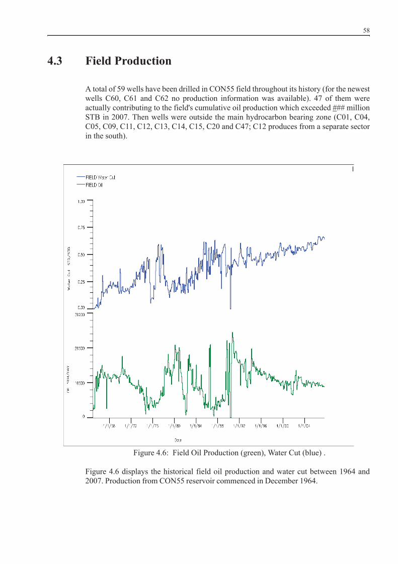
58
4.3 Field Production
A total of 59 wells have been drilled in CON55 field throughout its history (for the newestwells C60, C61 and C62 no production information was available). 47 of them wereactually contributing to the field's cumulative oil production which exceeded ### millionSTB in 2007. Then wells were outside the main hydrocarbon bearing zone (C01, C04,C05, C09, C11, C12, C13, C14, C15, C20 and C47; C12 produces from a separate sectorin the south).
Figure 4.6: Field Oil Production (green), Water Cut (blue) .
Figure 4.6 displays the historical field oil production and water cut between 1964 and2007. Production from CON55 reservoir commenced in December 1964. with an averaged

59
4.4 Reservoir Pressure
The initial reservoir pressures of both blocks are hydrostatic, 2450 psia at the reference ofdepth 5100 ft SS. The pressure declined during the production from 1964 until 2008 to1500 psia in average. Figure 4.7 shows the static BHP’s for all wells. The high scatter inpressure data is an indicator for the existence of different pressure regions, which areseparated from each other by at least partially sealing interfaces e.g. faults. Based on thedifferent pressure behaviors the reservoir was divided in 9 pressure/volume regions,showed in Figure 4.2. Figure 4.8 is an example for this data separation. Figure 4.9 showsthe average pressure development for all volume regions. At the end of 2008 the pressureis with 1000 psia the lowest in the middle of the reservoir (regions 7) and with 2000 psiathe highest in North (region 12).
Figure 4.7: Static BHPs of all wells of entire #W Block.
Kotla ReservoirStatic BHPs of All Wells of Entire Wasat Block
0
500
1000
1500
2000
2500
3000
Jan/ 63 Jan/ 73 Jan/ 83 Jan/ 93 Jan/ 03
Date [-]
Sta
tic P
ress
ure
at 5
100
ftSS
[psi
a]

60
Figure 4.8: Static pressures of wells within region VR_9.
Figure 4.9: Average pressures for individual segments and HCPV weighted reservoir pressure for the entire field.
Kotla ReservoirAvg. Region Pressures of VR_9 and Static BHPs of Wells C3, C7, C21, C23, C54 and C55
0
500
1000
1500
2000
2500
3000
Jan/ 64 Jan/ 74 Jan/ 84 Jan/ 94 Jan/ 04
Date [-]
Pres
sure
@ 5
100
ft SS
[psi
a]
Static BHPs Average of BHPs in 2 Year Intervals Interpolated Average
Average Reservoir Pressure of Kotla Field
0
500
1000
1500
2000
2500
3000
January 1964 January 1974 January 1984 January 1994 January 2004Date
Pre
ssur
e @
510
0 ftS
S [p
sia]
VR_2 VR_3 VR_4 VR_12 VR_8 VR_9 VR_17 AVERAGE VR_5 VR_7

61
4.5 Water Influx
Material Balance calculations on the bases of the volumetrically calculated OOIP,historical production and average reservoir pressures resulted in a water drive index of >0.8. The calculated water influx from the outer aquifer was around of 250 MMstb. TheFetkovich type analytical aquifer model gave the best fit. The material balance calculationdoes not define from which side the water was coming. In spite of the existence of mobilewater below most of the wells, the general character of the depletion is not a bottom waterdrive. Regarding most of the wells the main flow direction is in lateral direction.Regarding the reservoir structure given in Figure 4.1 and Figure 4.2 it seems to be surethat this can be quite uneven. To locate the water influx, the boundary must be segmented.
Figure 4.2 shows the boundary segments numbered from Bound1 to Bound11 astheoretical posibilities. After examining the lateral pressure gradients and the watering ofthe wells in detail the following boundaries were identified as active: Bound1, Bound3,Bound4, Bound6, Bound8 and Bound9.
4.6 Extracted Single Well Models
Caused by strong edge water inflow the CON55 wells do not posses individual drainageareas which could be regarded as an independent model. For this reason no HM can beperformed on single well models. In spite of that one grid cube and one cross section wereextracted by the author from the already matched full field grid at the position of the wellC18, shown in Figure 4.10 and Figure 4.12. The well C18 was selected because it ischaracteristic for the field, it has a long and continuous production history and operatesunder direct aquifer influence. The parameters within the the models were slightlymodified.
These two grid models will be used to examine certain behaviours and to explain theconcept and methods appied in the full field modeling. Note that these calculations aremodelings and not simulations. The results mirror the nature of the happenings, but do notoffer quantitative information about the well performances.

62
Figure 4.10: C18W well spots were extracted from the full field model .
Figure 4.11: 3D view of cross section model showing wells C18, C19 and C51, initial water saturation distribution and location of water influx boundary (red blocks) .

63
Figure 4.12: Initial saturation distribution of C18W single well model, with a cross section trough of the well.
The well model has an extent of 800 x 1050 m, and a thickness of 80 m average. The arealgrid size is 50 x 50 m. The model consists of 16x21x12 = 4032 grid cells. The model wasequilibrium initialized using the capillary pressure curve given in Figure 4.5. Figure 4.12shows the initial saturation distribution. The OOIP in this well spot model is 6.14 MMstb.On the right hand side, there is a boundary for water influx from the aquifer. Figure 4.13displays the production history of the well C18.
Both the single well model and the cross section is situated in volum region VR_17 (seefigure 4.2). The region pressures are displaid on Figure 4.9.
The cross sction model described in Figure 4.11 consists of 4548 blocks. The original oilin place equals 28.8 MMstb and the initial water volume equals 79.5 MMstb. The initialpressure was calculated to be 2439 psia. All wells produced with the historical oil andwater rates during the numerical experiments and the corresponding average regionpressure was defined as target pressure.

64
Figure 4.13: Production history of the well C18 and the target pressure assigned to the C18W model

65
Chapter 5
Validation of the Target Pressure and Phase Method
5.1 Introduction
This chapter describes the handling of the pseudo wells and their relation to thecorresponding real wells. It will be presented how pseudo wells can be used to match nearwell properties, fractures and coning behaviors. A single well and a cross section modelwill be presented to show that in certain cases the pseudo well is the only practicalsolution.
Nevertheless TPM is still an iterative procedure; the analytical aquifer parameters arevalid after all the wells produce exactly the historical rates of all components (in black oilmodel the oil, gas and water). For that, the model must be tuned. In a first step thegeological model will be revised (validated), then the production, PVT and SCAL dataare checked and corrected within the confidence range24, then also beyond that, followedby different kind of “pseudos” (e.g.: directional or perforation specific relativepermeabilities), interbeddings and low and high permeability strikes, baffles andchannels, but the goal will be never achieved26. Some differences between the model andreality always remain. At the end the reservoir parameters were tuned and the well modelwas adapted losing the confidence in both of them.
It is a justifiable question if the wells are identifiable and stable objects in a reservoirmodel or not. Already the localization of the effective well-reservoir connection isdifficult and the inflow performance changes by cement and casing failure, scaling etc.over time. The skin factors determined in subsequent tests can easily show 200% or 50%of the previous value. It makes no sense to try to model a well with constant parametersover longer time (10, 20 or 40 years), especially not for the history. A “matched well” hasno relevance.
The word “validation” in the chapter title is perhaps not the best expression at this place.The TPPM is not a mathematical model and not a solution which can be compared to

66
measurements, observations or results from other theoretical approaches. Nevertheless itis possible to explain the application of TPPM in more detail and to present simplified andeasier understandable cases. The objective of this chapter is to help the reader tounderstand the pseudo well concept and persuade him of its applicability.
In the following, three kinds of wells will be addressed:
• the real well which exists in the field,• the model well representing the real well in the reservoir model • the pseudo well, that masks the real well during the model building process.
The model well, as the name suggests, should represent the real well as good as possible.Amongst others, it should have the same trajectory and the same perforations as the realwell. Supplementary the calculation of the well inflow should be accurate, which requirescorrect analytical or gridded inflow models. Also if both, the reservoir and the wellmodels are the best possible ones, the linked reservoir well model will not fit the historicalproduction rates, GOR, WC and observed reservoir, bottom hole and well head pressures;at least not in the early stage of a modeling process. The objective of HM is to achievethat the rates, WC, pressures, etc. fit to the reality.
The main difference between the classical and the proposed approaches is easy to explain:
• In a classical approach, both the reservoir and the wells are “correctly” described buttheir modelled and measured behaviors will be different.
• In the new approach the pseudo well behaves as the real one, has the same rates, WC,pressures, e.t.c., but is different to the real well. The objective is to force the pseudowell to converge with the real one.
5.2 Well Models
5.2.1 Inflow performance
Wells can be represented in a reservoir model as simple volume sources, or as the wellknown Peacemen well model50,30 or at the end of the list as an independently griddedobject with skin zone, cement bound, casing, perforations, tubing, valves, pump and wellhead. Regarding the pseudo wells the most simple approach, namely the Peacemen wellmodel50,30 is certainly satisfactory.
The inflow rate of the phase p from a perforation (also called "connection" in Eclipse) Iwill be calculated by the following equation:
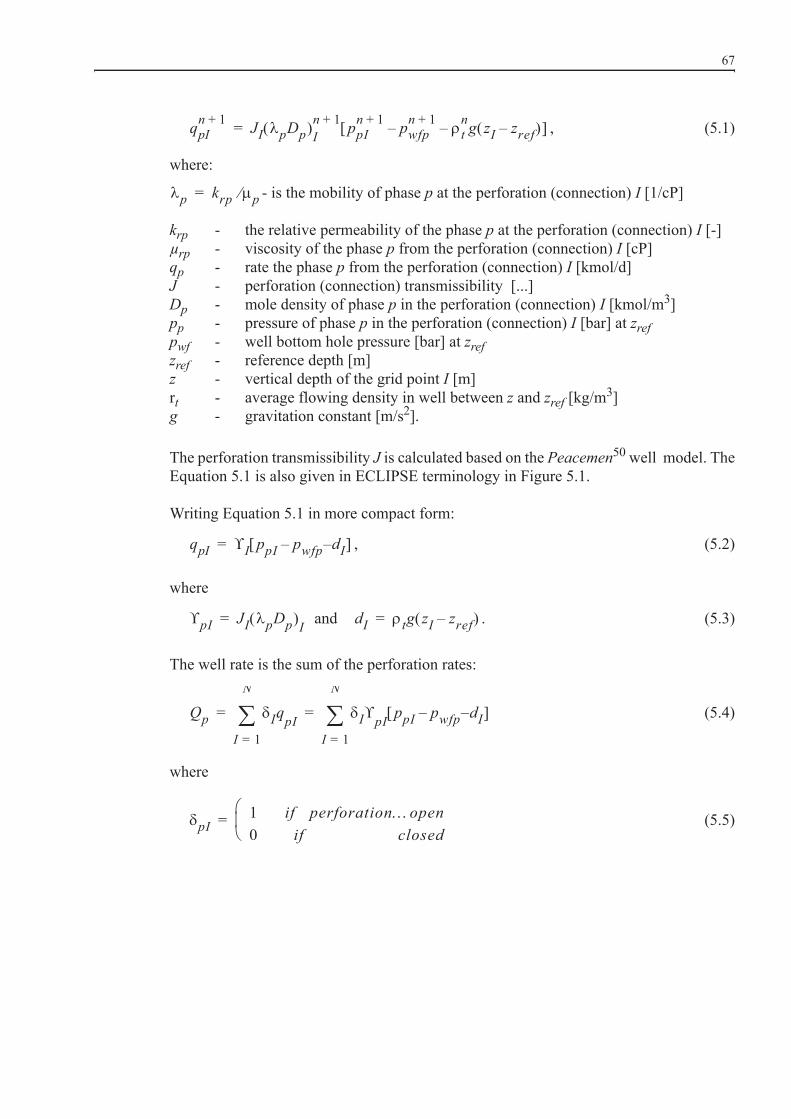
67
, (5.1)
where:
- is the mobility of phase p at the perforation (connection) I [1/cP]
krp - the relative permeability of the phase p at the perforation (connection) I [-] μrp - viscosity of the phase p from the perforation (connection) I [cP] qp - rate the phase p from the perforation (connection) I [kmol/d] J - perforation (connection) transmissibility [...] Dp - mole density of phase p in the perforation (connection) I [kmol/m3]pp - pressure of phase p in the perforation (connection) I [bar] at zrefpwf - well bottom hole pressure [bar] at zrefzref - reference depth [m]z - vertical depth of the grid point I [m]rt - average flowing density in well between z and zref [kg/m3]g - gravitation constant [m/s2].
The perforation transmissibility J is calculated based on the Peacemen50 well model. TheEquation 5.1 is also given in ECLIPSE terminology in Figure 5.1.
Writing Equation 5.1 in more compact form:
, (5.2)
where
and . (5.3)
The well rate is the sum of the perforation rates:
(5.4)
where
(5.5)
qpIn 1+ JI pDp I
n 1+ ppIn 1+ pwfp
n 1+tng zI zref–––=
p krp p=
qpI I ppI pwfp dI––=
pI JI pDp I= dI tg zI zref–=
Qp IqpII 1=
N
I pI ppI pwfp dI––I 1=
N
= =
pI1 if perforation open0 if closed
=

68
(5.6)
During the history match the oil, water and gas rates (Qo,Qw,Qg) are known. The free gasrate (QFg) can be estimated from the gas rate and the average pressure in the drainage area:
. (5.7)
Now three different bottom hole pressures can be calculated shown in Equation 5.6 whichare non-physical values. In the classical approach a single bottom hole pressure will becalculated using net or wet reservoir rates as target. The model well is operated normallywith target wet rate by water drive and by target reservoir volume by solution gas orgascap drive. For target wet rate the bottom hole pressure is:
(5.8)
The apparent bottom hole pressure and the calculated WC and GOR are the measures ofthe HM quality.
(5.9)
Figure 5.1: Inflow performance relationship in ECLIPSE 100 (from Eclipse Manual58)
pwfp
I pI ppI dI– Qp–I 1=
N
I pII 1=
N-------------------------------------------------------------=
QFg Qg QoRs p–=
pwfb
I o w+ I poI dI– Qb–I 1=
N
I o w+ II 1=
N-------------------------------------------------------------------------------=

69
5.2.2 Productivity Index
To calculate the BHP on the bases of the perforation parameters is relatively uncertain andis difficult the verify. Production logging will be rarely made and the results also havelimited validity over time. In contrary to this, production tests will be carried out often andthe productivity indices of the wells are regarded as being known all the time:
. (5.10)
where
. (5.11)
and Q is the reservoir volume rate of the well (in a single phase case also surface rate canbe used) and is the static well pressure. The target bottom hole pressure is then:
, (5.12)
where both and pBHP are calculated at the reference depth. The well by well pressurematching can be based only on these three quantities: Q, p and pBHP. The BHP can bemeasured directly, the reservoir rate can be calculated with confidence, especially in theabsence of free gas. Measuring static pressures is sometimes delicate but there is noalternative.
The static pressures will not be calculated in a numerical reservoir model either. They willbe estimated using questionable averaging methods as WPAVE in ECLIPSE58. But at theend of the day these two pressures ( and pav) will be compared and regarded as measureof the HM quality. Klima36 suggested that the comparison should be constraint by the PI,regarding it as realistic and hard data. From a practical point of view it is better todetermine or estimate the productivity indices and to use them to improve the quality ofthe history match.
5.2.3 Estimation of perforation rates
At this point the calculated phase bottom hole flowing pressures from Equation 5.4 aredifferent for the phases. This discrepancy can be eliminated by tuning the transmissibilityof the perforations. The following procedure was suggested by Klima36.
Consider the time period <ta,tb> in which no recompletions took place, the productivityindex PI is known (and can be regarded as constant) and the (pseudo-) perforations werenot changed. Choose K time step within this period (the number of time steps in the period
PI Qp
-------p 0–lim=
p p pBHP–=
p
pBHP p QPI------–=
p
p

70
is > K). Depending on the number of mobile phases 1 to 3 equations can be written for theK timesteps according to Equation 5.4. If all quantities in this equation would be realisticand exact, then the difference in phase bottom hole pressures would be the capillarypressure only. This difference is small, can not be measured (and so can not be verifiedeither) and therefore it should be neglected27:
. (5.13)
The common BHP results from Equation 5.12: (5.14)
(5.15)
where PI is taken from production tests and is calculated by the averaging method inuse (WPAVE option). Equation 5.4 can be written in a compressed form:
, , (5.16)
where
. (5.17)
In this work the case with 3 mobile phases (with free gas) was not really handled, also heretwo phases, oil and water will be considered. Writing Equation 5.18 for this phases 2*Kequations will be achieved containing N unknowns where N << 2*K:
(5.18)
(5.19)
Not that this equations brought the measurements (PI) and the well model to a commondenominator.
In Equation 5.5 I equals 1 if the perforation is open and 0 if not. Now it is suggested toregard dI as a correction factor for the perforation. The Equation 5.18-Equation 5.19should be valid over a longer time period with the smallest possible errors, keeping ’sconstant. The unknown in these equations are therefore the perforation transmissibilitymultiplier I.
They can be determined solving the Gauss normal equations:
pBHPoj pBHPwj pBHPgj pBHPj= = =
pBHPj pj
BoQo BwQw BgQFg+ +j
PI-----------------------------------------------------------------–=
pj
epIj II 1=
N
Qpj= j 1 K=
epIj pI ppI dI pBHP–– j=
ewIj II 1=
N
Qwj=
eoIj II 1=
N
Qoj=
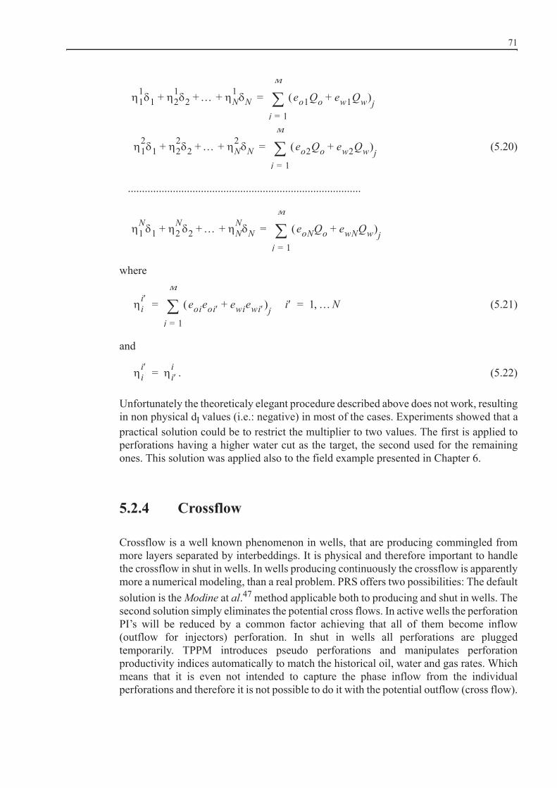
71
(5.20)
...................................................................................
where
(5.21)
and
. (5.22)
Unfortunately the theoreticaly elegant procedure described above does not work, resultingin non physical dI values (i.e.: negative) in most of the cases. Experiments showed that apractical solution could be to restrict the multiplier to two values. The first is applied toperforations having a higher water cut as the target, the second used for the remainingones. This solution was applied also to the field example presented in Chapter 6.
5.2.4 Crossflow
Crossflow is a well known phenomenon in wells, that are producing commingled frommore layers separated by interbeddings. It is physical and therefore important to handlethe crossflow in shut in wells. In wells producing continuously the crossflow is apparentlymore a numerical modeling, than a real problem. PRS offers two possibilities: The defaultsolution is the Modine at al.47 method applicable both to producing and shut in wells. Thesecond solution simply eliminates the potential cross flows. In active wells the perforationPI’s will be reduced by a common factor achieving that all of them become inflow(outflow for injectors) perforation. In shut in wells all perforations are pluggedtemporarily. TPPM introduces pseudo perforations and manipulates perforationproductivity indices automatically to match the historical oil, water and gas rates. Whichmeans that it is even not intended to capture the phase inflow from the individualperforations and therefore it is not possible to do it with the potential outflow (cross flow).
11
1 21
2 N1
N+ + + eo1Qo ew1Qw+ jj 1=
M
=
12
1 22
2 N2
N+ + + eo2Qo ew2Qw+ jj 1=
M
=
1N
1 2N
2 NN
N+ + + eoNQo ewNQw+ jj 1=
M
=
ii eoieoi ewiewi+ j i
j 1=
M
1 N= =
ii
ii=

72
Therefore the second PRS solution will be applied only. The perforation multipliersdetermined by TPPM contain this kind of "cross flow factor" too.
5.3 Pseudo Wells
5.3.1 Setting of pseudo wells
Every history matching follows a hierarchical approach, going step by step from theglobal pressure match through the regional match to the well by well match. This workintroduced an intermediate unit, called well spot, between the regions and the wells,representing more or less the drainage area of a well. Supplementary to the real wells,pseudo wells are introduced into the well spot. A pseudo well can, but does not have to bebe, different from the real well. This means that it can have a different location, differentperforations and artificial near well parameters as productivity indices, etc.. The onlyrequirement for the pseudo well is, that it must be able to produce the same oil, gas andwater rates as the real well all the time.
Generally it is no restriction how a pseudo well should be set. As already mentioned theobjective of the matching process is to force the pseudo well to converge with the real one.Therefore the pseudo well should contain the real perforations in any cases. Thesupplementary perforations, called pseudo perforations, can be set along or on theextension of the real well trajectory, but they can also be arbitrarily distributed within thespot. In case of vertical wells, all layers above and below the real perforations should bedeclared. In case of horizontal wells also blocks outside of the trajectory laying in thevertical and/or in the horizontal plain can be considered. Generally speaking the well willbe regarded as a pseudo multilateral well, having access to its entire drained reservoirvolume if necessary. All these pseudo perforations should be introduced, for reasons ofdata management into the simulation software, at the model initialization and then beclosed. They will be activated later if necessary.
The target phase rates will be distributed individually among the perforations based onEquation 5.4. Consequently two (or three) bottom hole pressures (BHP) will be obtained,differently for oil, water (and gas). The result is naturally not physical, but this is also notrequired at this stage. Important is only that all wells produce the reported rates over theentire history. If this is possible, then there is enough mobile oil, water and gas at the realperforations all the time and the model is globally right. If this is not the case, then thepseudo perforations can be opened one after one. If the well can not be operated even insuch a way, then the available amount of oil, water and gas globally or locally isinsufficient.
To be able to complete the actual run, the problem wells will be switched to wetrat control.Also the low permeability can constrain the wells by minimum bottom hole pressure.

73
Perforation transmissibility multipliers will be applied automatically to keep the modelwells in operation. Note that as consequence of the ptarget option the reservoir pressureis always correct.
What the TPPM approach can do at this stage is easy to explain: The run informs the userwhich well construction (location and PI’s of perforations) could produce the historicalrates with the measured BHP at the offered reservoir structure and parameters within theindividual spots (drainage areas). TPPM opens and closes pseudo perforations and assignsmultipliers to the individual perforations to match the targets. The solution is naturally notunique. Therefore PRS offers options as matching, stretch, extend, average, forced,WPIMULT, WPIMULTP, with which the user can influence and constrain the automaticmatching. In this way the TPPM provides pseudo wells telling the user “if your reservoirspot looks so then I would need such a well to produce as happened.” If the pseudo welldiffers considerably from the real well, than the reservoir geology must be updated. Thequality measures of the reservoir description are the artefacts in the tuned pseudo wells.The objective of the fine re-parametrization of the reservoir model is to eliminate or atleast to reduce the number (extension) of the pseudo perforations. In TPPM it is (shouldbe) still forbidden to tune the dynamic model at this level of the project.
5.4 Single Well Modeling
The CON55 field operates under strong edge water drive. This was already established byconceptional models by Mittermeir et al41. Low and high permeable strikes, also if theycould not correlate between the wells lead to early water break trough in structurallyhigher perforations.
In such a situation a well does not posses an individual drainage area, which could beregarded as an independent model. For this reason, no HM can be performed on CON55single well models. The following calculations are therefore modeling and not simulation.The results mirror the nature of the happenings, but do not offer quantitative informationabout the well performances. In clear words, this chapter presents model calculations onthe selected wells but not a simulation.
To keep the connection to the actual reservoir as close as possible the well C18 wasselected for investigation and demonstration. The well spot, shown in Figure 4.10, wasextracted from the already matched full field model. At the right hand side of the grid,there is the boundary to the aquifer.
The well C18 is situated in volume region VR_17 (see figure 4.2). Their average pressure,displayed on Figure 4.9, is used as target pressure. Figure 4.13 shows the historical oil andwater productions.
Two grid models were applied:-
1. Cartesian grid, as in the full field model.
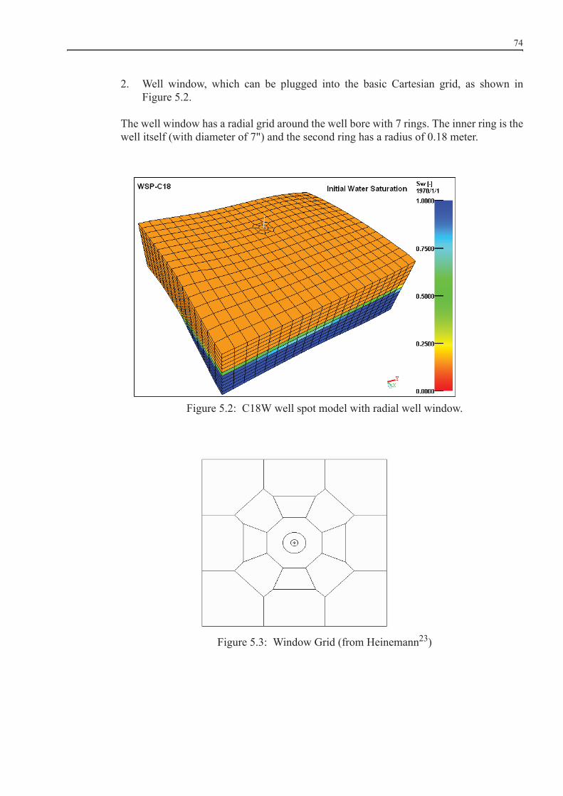
74
2. Well window, which can be plugged into the basic Cartesian grid, as shown inFigure 5.2.
The well window has a radial grid around the well bore with 7 rings. The inner ring is thewell itself (with diameter of 7") and the second ring has a radius of 0.18 meter.
Figure 5.2: C18W well spot model with radial well window.
Figure 5.3: Window Grid (from Heinemann23)
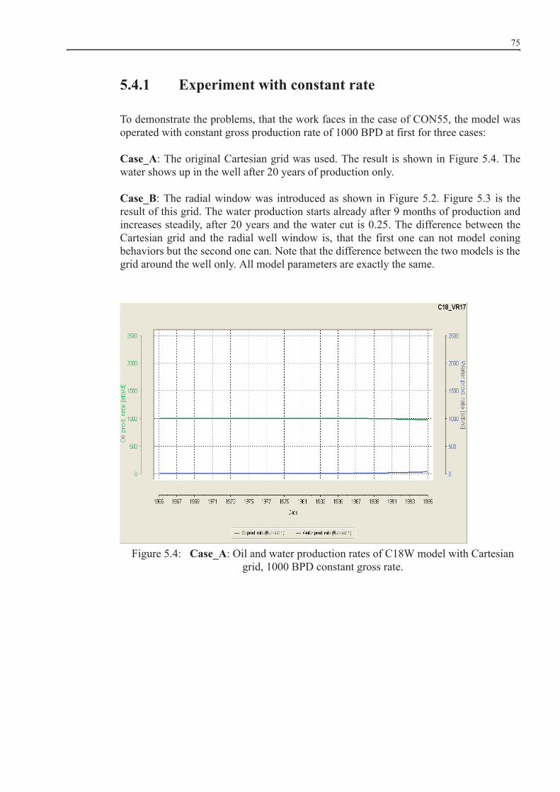
75
5.4.1 Experiment with constant rate
To demonstrate the problems, that the work faces in the case of CON55, the model wasoperated with constant gross production rate of 1000 BPD at first for three cases:
Case_A: The original Cartesian grid was used. The result is shown in Figure 5.4. Thewater shows up in the well after 20 years of production only.
Case_B: The radial window was introduced as shown in Figure 5.2. Figure 5.3 is theresult of this grid. The water production starts already after 9 months of production andincreases steadily, after 20 years and the water cut is 0.25. The difference between theCartesian grid and the radial well window is, that the first one can not model coningbehaviors but the second one can. Note that the difference between the two models is thegrid around the well only. All model parameters are exactly the same.
Figure 5.4: Case_A: Oil and water production rates of C18W model with Cartesian grid, 1000 BPD constant gross rate.

76
Figure 5.5: Case_B: Oil and water production rates of C18W model with radial well window;, 1000 BPD constant gross rate.
Figure 5.6: Case_C: Oil and water production rates of C18W model with radial well window and vertical fracture; 1000 BPD constant gross rate.
77
Case_C: It is assumed that CON55 is partly fractured, especially near to faults. Suchfractures can enhance the productivity index considerably, as it was observed with manywells (also in C18), but they could be responsible for early water break through and highwater cut also.
To simulate a possible vertical fracture the vertical permeability in the 2nd and 3rd ringwas increased by a factor of 100.
This approximates a fracture with 0.6 m half-length and 1 mm width. Such a fracture hasaccording Lamb's law 84400 Darcy of permeability (from Aziz6). This construction is notabsolutely correct (theoretically it would be possible to grid the fracture too) but it is nearto the perception.
The result is shown in Figure 5.6. The water breaks into the well within some months, thewater cut is above 0.40 after one year and increasing to 0.50 after 20 years. Note that thenature of the watering in this case seems to be similar to the historical behavior of the realwell C18, given in Figure 4.13.
Figure 5.7 compares the cases A, B and C. Assuming that the production in Case C is the“historical” one, two questions can arise:
1. Does TPPM match the history without introducing a radial well window andwithout assuming vertical fractures in vincinity of the well?
2. Can the matched model predict the future performance of “historical” model?
If the answer is no, than TPPM can be forgotten.
Case A was re-calculated with TPPM, taking the production from Case C as “historical”.Figure 5.7 displays the oil and water rates for Case A, the “historical” Case C (light greenand blue) and Case A with TPPM (dark green and blue).
The two last cases are nearby identical, so it must be shown in a magnification that thereare some numerical differences. The number of pseudo perforations below the real onesis 5 at the beginning, then 4 and 3 at the end.
In the actual set up the transmissibility multiplier was applied to the deepest perforation,the other ones were multiplied with the reciprocal values. Figure 5.8 displays the numberof perforations and the multipliers.
The “pseudo well” matched over 25 years could be used to predict the following 5 yearswith a fixed number of pseudo perforations and with constant multipliers.
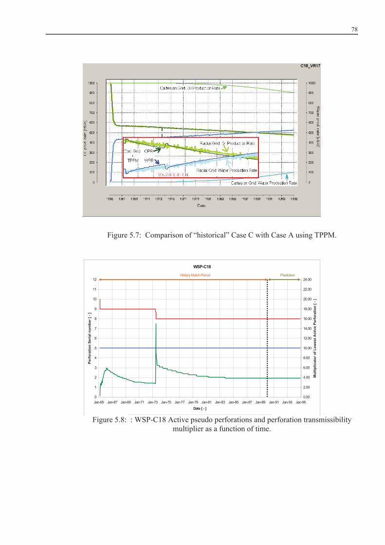
78
Figure 5.7: Comparison of “historical” Case C with Case A using TPPM.
Figure 5.8: : WSP-C18 Active pseudo perforations and perforation transmissibility multiplier as a function of time.
WSP-C18
0
1
2
3
4
5
6
7
8
9
10
11
12
Jan-65 Jan-67 Jan-69 Jan-71 Jan-73 Jan-75 Jan-77 Jan-79 Jan-81 Jan-83 Jan-85 Jan-87 Jan-89 Jan-91 Jan-93 Jan-95
Date [ - ]
Perf
orat
ion
Seria
l num
ber [
- ]
0.00
2.00
4.00
6.00
8.00
10.00
12.00
14.00
16.00
18.00
20.00
22.00
24.00
Mul
tiplic
ator
of L
owes
t Act
ive
Perf
orat
ion
[ - ]
History Match Period Prediction
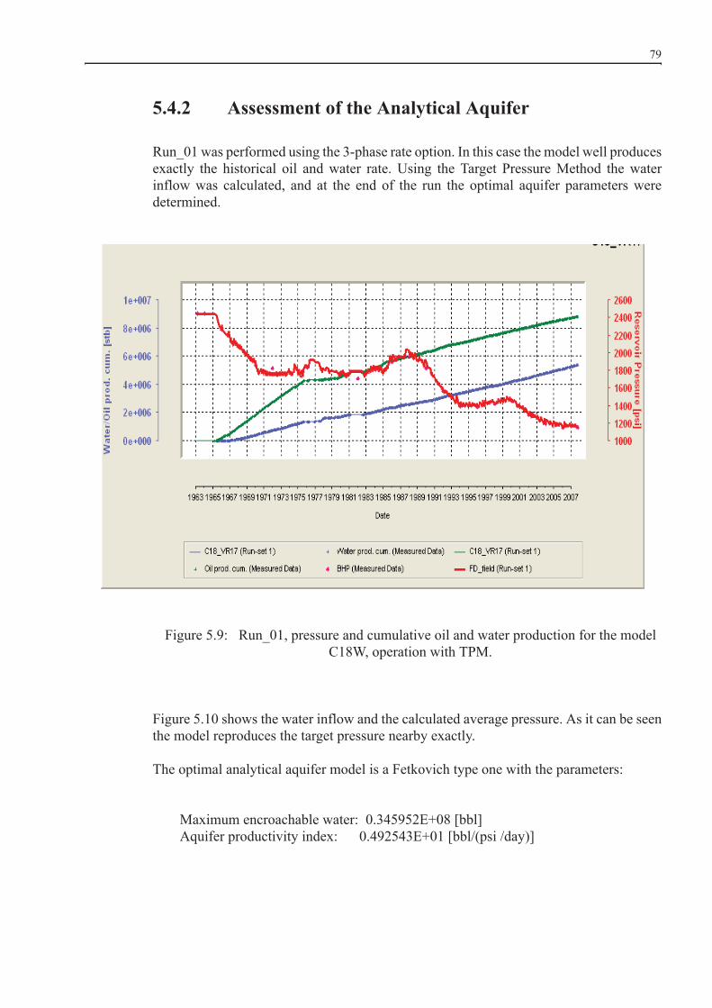
79
5.4.2 Assessment of the Analytical Aquifer
Run_01 was performed using the 3-phase rate option. In this case the model well producesexactly the historical oil and water rate. Using the Target Pressure Method the waterinflow was calculated, and at the end of the run the optimal aquifer parameters weredetermined.
Figure 5.9: Run_01, pressure and cumulative oil and water production for the model C18W, operation with TPM.
Figure 5.10 shows the water inflow and the calculated average pressure. As it can be seenthe model reproduces the target pressure nearby exactly.
The optimal analytical aquifer model is a Fetkovich type one with the parameters:
Maximum encroachable water: 0.345952E+08 [bbl]Aquifer productivity index: 0.492543E+01 [bbl/(psi /day)]

80
Figure 5.10: Run_02, result of C18W model operating with analytical aquifer.
The results of Run_01 and Run_02 show that the model is suitable for the plannedinvestigations; the spot can produce the desired amount of oil and water under the givenpressure history.
5.4.3 Experiments with Historical Production Rate
The exercise is now to match the production as closely as possible using the single wellmodel. Note that all reservoir parameters, except the permeability, are equivalent to thosein the geomodel. Naturally it would be advantageous to use the windowing technique, butthis is not available in ECLIPSE. Therefore the Cartesian grid is the only real possibility.The match could be done as usual, i.e. the match could be performing by tuning some ofthe following parameters in the model:
• Horizontal permeability• Vertical permeability• Introducing layering, high and low permeability streaks• Initial saturation distribution• PI's for the perforations• Relative permeability • Capillary pressure

81
Figure 5.11: First attempt to match C18 by changed horizontal and vertical permeability
Figure 5.12: Tenth attempt to match C18 by changed horizontal and vertical permeability.
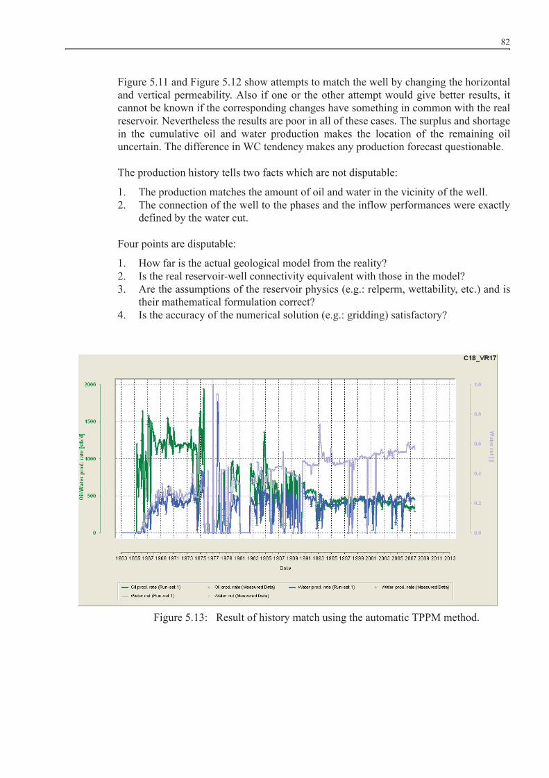
82
Figure 5.11 and Figure 5.12 show attempts to match the well by changing the horizontaland vertical permeability. Also if one or the other attempt would give better results, itcannot be known if the corresponding changes have something in common with the realreservoir. Nevertheless the results are poor in all of these cases. The surplus and shortagein the cumulative oil and water production makes the location of the remaining oiluncertain. The difference in WC tendency makes any production forecast questionable.
The production history tells two facts which are not disputable:
1. The production matches the amount of oil and water in the vicinity of the well.2. The connection of the well to the phases and the inflow performances were exactly
defined by the water cut.
Four points are disputable:
1. How far is the actual geological model from the reality?2. Is the real reservoir-well connectivity equivalent with those in the model?3. Are the assumptions of the reservoir physics (e.g.: relperm, wettability, etc.) and is
their mathematical formulation correct?4. Is the accuracy of the numerical solution (e.g.: gridding) satisfactory?
Figure 5.13: Result of history match using the automatic TPPM method.

83
What could be done?
Twist the reservoir and the physics or, admit that in certain cases the reservoir engineeringscience and practice is not able to say how the phases are distributed in the reservoir andhow the well gets access to these.
It is better to let the well do, what it has to do and to accept, that the model failed to explainhow it works.
Figure 5.13 shows the result of the match based on TPPM concept. The match cannot bebetter. As it can be seen, no such changes were allowed during the last 5 years, so thecredibility of the forecast is assured. The possibility to optimize the well construction withthis approach is not given.
The author believes that the water production in most of the CON55 wells is influencedby the combination of the following factors:
extended transition zones, heterogeneous initial water saturation,fractional wettability,water coning,fractures andlateral water encroachment.
All these factors should be investigated further, to bring the analytical and the simulationmodels close to each other. The ideal situation in which a model satisfies bothrequirements will be never achieved.
5.5 Applicability of TPPM to Stratified Reservoirs
5.5.1 The Objective
Many different displacement patterns and processes can take place within a reservoir. Theactual recovery processes can be regarded as a superposition of many individual processeshappening at the same place concurrently. The aim of the full scale reservoir simulationmodel is to reproduce this complex recovery process. Just one example will be mentionedhere. For volume region VR_17 water encroachment takes place concurrently from theNorth and from the East. Thus the individual North-South and East-West displacementsare blurred out. Consequently a full scale model is not suitable for investigating anddemonstrating the individual recovery processes. For such detailed studies specializedmodels like column, single well and cross section models are required.
Previously it was pointed out, that from the hydrodynamic point of view no distinct

84
zonation for the CON55 Reservoir could be established. To be more precise, the zonesG1-G7 identified during the creation of the 3D reservoir model based on lithostratigraphicwell correlations did not indicate any vertical flow barriers or high permeability streaks.Nevertheless, such features cannot be excluded for CON55 Reservoir. Contrary, due to thecomplex water cut history of CON55 wells it is likely that such features exist, even if theycould not be detected on well logs or seismic data.
Despite the likeliness and production data induced indications for the existence of verticalflow restrictions and/or high permeable channels, no information about their latter andvertical position and extent is available. Consequently it is not possible to introduce suchfeatures in the full scale simulation model.
Nevertheless the presented history match was able to reproduce the complex measuredwater cut history very accurately. The applied methodology was presented in Chapter 3.
The author conducted model calculations on a cross section model extracted from CON55full scale model to demonstrate the impact of vertical flow restrictions and high permeablestreaks on the displacement process. This Section and its Subsections will describe thesemodel calculations in detail.
5.5.2 Model Setup
To demonstrate the displacement process in case of the existence of vertical flowrestrictions and high permeable streaks a cross section model along the wells C18, C19and C51, which are all situated in a row in West to East direction was extracted from thefull scale model. A 3D view of this cross section model can be found in Figure 4.11duplicated in this chapter by Figure 5.14. The coloring is chosen to show the initial watersaturation distribution. Additionally the location (red blocks) of an outer boundary, actingas source for water influx from an outer analytical aquifer is shown. Despite the 3Dcharacter of the model displayed in Figure 5.14 it can be regarded as a cross section andnot as a sector model, due to the fact that the displacement takes place only in two and notin three dimensions. The presented model calculations could be also conducted on a strict2D cross section model, but in this case major alterations compared to the full scale modelwould have been necessary to operate the model in the desired way. For a 2D model theamount of original oil in place would be definitely too small to let produce the wells C18,C19 and C51 at their historical liquid rates. The author's goal was to keep the overall setupof the cross section model as close as possible to the full scale model. Only a limitednumber of minor alterations was introduced to enhance the effects that should bedemonstrated with this type of model.

85
Figure 5.14: 3D view of cross section model showing wells C18, C19 and C51, initial water saturation distribution and location of water influx boundary (red blocks).
The cross section model in use is characterized by the following issues:
• Top and bottom structure, as well as the layering are exactly those of the full scalesimulation model.
• The wells are at their real positions, produce their historic liquid rates and thecompletions of wells C19 and C51 are identical in position and time sequence to thereal ones.
• Contrary to wells C19 and C51 the completion interval for well C18 was not changedover time for the model calculations. For demonstration purposes well C18 wascompleted in the second and third simulation layer only. The real perforation wouldbe situated in the third and forth layer.
• Porosity and net-to-gross ratio was not altered compared to the full scale model.
• The lateral permeability equals 250 mD throughout the entire cross section model.Only for the third simulation layer the lateral permeability was increased by onemagnitude.
The resulting transmissibility distribution in x-direction is shown in Figure 5.15. Despitethe constant lateral permeability and the nearly invariable cell height, variations intransmissibility can be observed from Figure 5.15. These variations are solely theconsequence of the stochastic net-to-gross ratio distribution. The artificially introducedhigh permeability streak can be identified by the sequence of red blocks.

86
Figure 5.15: Cross section along wells C18, C19 and C51 showing lateral transmissibility distribution .
The vertical permeability equals 2.5 mD throughout the entire cross section model.Between the third and the fourth layer a vertical flow restriction was introduced bydecreasing the transmissibility in z-direction by two magnitudes across this cell interface.This is indicated by the purple blocks in the third layer of Figure 5.16.
Figure 5.16: Cross section along wells C18, C19 and C51 showing vertical transmissibility distribution .
The chosen cross section is delineated by sealing faults at the West and at the East side inthe full scale model. For the cross section model calculations this sealing character waskept for the West edge, but not for the East. Towards the East a boundary acting asinterface for an outer analytical aquifer was attached. The location of this boundary isindicated by the red blocks in Figure 5.14. To achieve a closure towards this boundary, thefree water level was set to 5248 ft SSL instead of the 5268 ft SSL of the full scale model.PVT and SCAL data equals those of the full scale model. The entire cross section modelbelongs to the first rock region.
The model described in Section 0 consists of 4548 blocks. The original oil in place equals40.7 MMstb and the initial water volume equals 66.7 MMstb. The initial pressure wascalculated to be 2446 psia. The model was operated for the entire history period of CON55reservoir. All three wells were able to produce their historic liquid rates but the oil andwater rates were naturally different.

87
One of the objectives of the Case_I was to demonstrate how the displacement wouldbehave in the presence of a clear vertical flow restriction, respectively lateral highpermeability streak. Both features act in a similar manner. They allow the encroachingwater to override the oil. This overriding and the resulting stratified saturation distributioncould be clearly demonstrated by the conducted cross section model calculations. Toenhance the significance of such a displacement process, both features, the vertical flowrestriction and later high permeability streak were combined into a single model.
Figure 5.17 presents the results of these model calculations Case_I. It displays the watersaturation distribution at five distinct time points. At the top the initial state is presented.Due to the flow conduit in the third layer, water encroaching from the analytical aquiferattached to the Eastern model boundary tends to override the oil. This tendency can beobserved on the subsequent cross sections.
Wells C18 and C19 both started to produce in mid 1965. Already half a year later theoverriding effect can be observed (second picture from top in Figure 5.17). The longer thedisplacement process takes place, the more pronounced the overriding effect becomes,until the layers at a distinct column location are equally flooded.
Figure 5.17: Water saturation distribution alterations for cross section model having a vertical flow restriction and a high permeability streak.
This model allows an experiment. The result should be regarded as “historical” and thereservoir parameters should be modified now in two directions:
1. Case_II: Influencing the phase distribution near the wells only: The highpermeability streak and vertical barrier was taken out.
2. Case_III: Altering the phase distribution regionally: The permeability in the leftupper side of the model (blocks I=1-56 from 106, K=1-6, from 12) was reduced byfactor 10.

88
If the TPPM can provide what was promised, then in the first case it should be able toreproduce the history, in the second case not.
Figure 5.18 show the result of Case_II. The dots are the results of Case_I. As it can beseen, the two results are practically identical.
Figure 5.19 shows the result of Case_III. TPPM tried to do its best but a match was notachievable by using pseudo perforations and multipliers only. The model is still notmatched globally.
In a situation as Case_II the modeler can switch to the “well_by_well” match, performinglocal parameter tuning. This cannot be done in Case_III. Also in Case_II it should be clearthat not only the reservoir parameters are the question, but also the numerical methods inuse. It can be easily seen, that with an improved discretization (orthogonal an unstructuredPEBI grids, grid refinement, optimal layering) the pseudo perforations would besuperficial.
Figure 5.18: Cumulative oil and water production of the wells in Case_I (dots) and Case_II (continuous).

89
Figure 5.19: Cumulative oil and water production of the wells in Case_I (dots) and Case_III (continuous).

90
Chapter 6
Full Field Application of TPPM
6.1 Introduction
This chapter presents the first successful field application of TPPM. The project wasconducted by HOL following a conventional History Matching approach and by usingECLIPSE simulation software. This was a fundamental obligation because the operatingcompany requested the use of ECLIPSETM black oil simulator for this study but let openthe possibility to apply also other tools under the condition that all of the finalized inputdata will be prepared as ECLIPSE input files and run on the Company's computers.
Most of the TPPM algorithms were developed while working on the full field model. Thepractice showed that after all small test examples worked fine, already 3 to 5 times morework was necessary to succeed with the real field example. Supplementary months wereinvested to generalize the code and to test it. The implementation of TPPM in PRS andthe connected programing work was not done by the author, his merit and responsibilityis limited to develop the concept and to the test the software.
The HM work needed 8 months in total (HOL worked on more projects in parallel). Inhalf of the time ECLIPSE was used only. Later on PRS become the master tool. In the lastcycle, after a final update of the geological model, only PRS was used until the end of HM.Then the PRS model was converted to ECLIPSE, making the predictions with it. It wasnot necessary to make any fine tuning on the PRS matched model, the results on ECLIPSEwere practically identical.
In the following the field case will be presented in a “idealized” manner, as if the workflow would be applied from the beginning already. The goal is not to show the strugglingduring the development but to give an example for future applications.

91
6.2 History Matching Workflow
After setting up the first structural model, a 50x50 m areal grid with 84 layers has beenconstructed and parameterized. The question was how many simulation layers will benecessary and optimal. The model showed strong heterogeneities but no lower or higherpermeability strikes could be correlated between the wells. On top of that, no separationsurfaces could be identified. Therefore it was decided to upscale the model to 12proportional simulation layers.
The 12 layer model with 137.400 active grid blocks was used for the conceptualmodelling and for the history matching. The area was divided into 9 volume regions:VR1, VR2, VR3, VR4, VR17, VR7, VR8, VR9, and VR12 as shown in Figure 4.2. Thewell names were extended by the corresponding region names for easier orientationduring the work (e.g.: C8_VR9 is a well in region 9). Boundaries were defined connectingthe reservoir to outer aquifers. From the initially assumed 11 aquifer connections, 6 wereproved to be active. They are Bound1, Bound3, Bound4, Bound6, Bound8 and Bound9.
It is always necessary to define a priori under which conditions the HM can be regardedas successful and applicable for forecasting. The results of a HM are the averagepressures, static and dynamic BHP for wells, the cumulative oil, water and gas productionand the production rates at the end of the history period. Which items are more importantin a given case depends on the nature of reservoir, the depletion mechanisms and - verystrongly - on the objective of the study. These limits are case dependent. It depends on theavailability and quality of the data, on the quality of the geomodel and on the time frameof the study. The limits defined for the actual study are given in Table 6.1 and Table 6.2.The allowed difference in cumulative production on field and volume region level is givenin absolute numbers (+/- MMstb) and also in percentage (%).
The production started in December 1964 and the end of HM was August 2009. Thehistory match was conducted in three steps.
Table 6.1: Error limits field production
Table 6.2: Error limits for average pressures
oo +/-
MMstb o %Oil 3.0 2%
Water 5.0 3% Liquid 1.0 0.50%
oo field
level o volume regions
level Maximum 150 psia 100 psia
At the end of history 100 psia 50 psia

92
Step 1: Conceptual modeling and global matching
The main goal of this step was to constrain the static model and to avoid realizationswhich at the end of the day contradict the production history. The TPPM was used withthe target pressure (ptarget) and the pseudo well (ph3rat)options. The explanation TheTPPM assessed the water influx by closely matching the historical regional pressures andthe oil and water production by activating pseudo perforations. This approach operates 2wells instead of one at every well location: one produces oil, the other one water andcalculates two bottom hole pressures. 32 from the 47 wells could be operated withhistorical oil and water rate over the entire 45 year period in the first run already. Basedon the hints resulting from the simulation work the following improvement could be donein the geomodel:
• The reservoir top was corrected in the surrounding of the wells C35, C45 and C46, butwithout changing the well tops itself, which were strictly honoured as hard data.
• The original assumption that the NTG ratio is 1.0 was dropped. The actual average isnow 0.87.
• Sub-seismic faults were identified between the volume regions VR_12 and VR_9 andVR_8 and VR_9. The position and extent of the volume regions can be found inFigure 4.2.
At the end of this step all wells were operated with the historical oil and water rates. Notethat at this stage the global match is finalized. The reservoir pressure is matched for allvolume regions producing exactly the historical oil and water rates during the entire HMperiod. Also the general setup of the simulation model was fixed as shown in Figure 4.2.This map contains all important elements: Faults, boundaries, regions and wells. Thecalculations confirmed the assumption made in material balance calculations, that the bestsolution can be achieved using Fetkovich type aquifer models.
Step 2: Spot by spot matching
The TPPM was used with the options ptarget, ph3rat and wetrat. Wells which becamecloser to be matched, were switched automatically from ph3rat to wetrat.TThe optionwetrat operates the wells in the usual manner, but opens pseudo perforations if necessary.At this stage only one bottom hole pressure, valid for both phases, is calculated. TheTPPM assessed the water influx by matching closely the historical regional pressures andthe water cut by introducing pseudo perforations and perforation transmissibilitymultipliers. In this history matching phase regional porosity and permeability multiplierswere applied and a supplementary rock region was introduced.
Step 3: Well by well matching.
In this step the target pressure method was not applied anymore. The water inflow wascalculated by analytical Fetkovich aquifer models, determined in Step 2. The wells wereoperated under wetrat and netrat production control. TPPM with the automatic tuning ofwell inflows was applied to less and less wells; at the end to none of them. Perforationtransmissibilities and near well reservoir properties were tuned in the usual - manual - wayto match the well production histories as close as possible. In some wells the perforation

93
intervals were still stretched or shortened to counterbalance grid effects (e.g.: coning) ornot identified geological objects or properties (e.g.: interbedding). The procedure endedup in a conventional dynamic reservoir model, running also on ECLIPSE, were none ofthe TPPM options exist.
6.3 Initialization
There were two possibilities to initialize the simulation grid model:
• Non-equilibrium initialization on the basis of the saturation distribution fromstochastic simulation.
• Equilibrium initialization based on capillary function, which can be different in everyrock region.
The author and HOL’s experts tried both possibilities, but then decided to go for thesecond solution. Figure 6.1 shows the two functions applied. The first one (green) wasconstructed from the log derived saturation distribution in the geomodel and tuned tobecome close to its OOIP. The second one (red) is an artefact and it was introduced duringthe history match to place more oil in certain regions. These regions are displayed inFigure 6.3.
Figure 6.1: Capillary pressure as a function of water saturation.
Kotla FieldCapillary Pressure Function
0.0
5.0
10.0
15.0
20.0
25.0
30.0
35.0
40.0
45.0
50.0
0.0 0.1 0.2 0.3 0.4 0.5 0.6 0.7 0.8 0.9 1.0
Sw [-]
Pcow
[psi
a]
Pcow for 1st rock region Pcow for 2nd rock region

94
The difference between the PA geomodel and the original simulation model, caused bythe different initialization methods, was 0.3 % only.. The geomodels were initializedbased on the stochastic water saturation distribution and the simulation models wereinitialized based on the capillary pressure functions.
As already written above, the geomodel was updated during the HM Step 1 already. Allcorrections were made by reinterpretation of seismic and log data and not by simpletuning. Further changes were made in the simulation model to enhance the HM. Thissection describes such kind of structural and parameter changes. Their geologicalrelevance would be proven at the end of the modelling work and integrated into the finalgeomodel whenever possible.
6.3.1 Structural Modifications
The original structure of the geological model was updated solely in three areas of theCON55 reservoir. History matching showed that the amount of OOIP in the vicinity ofwell C35, C45 and C46 was insufficient to be able to produce the historically measuredcumulative oil production from the simulation model. The objective of these structuralchanges was to lift the top structure within the uncertainty range inherent to seismicinterpretation without altering the well tops of the wells itself.
6.3.1.1 Faults
Based on the observations and conclusions drawn from the simulation model, it wasdetermined which faults or fault segments are sealing, partial sealing or open.
• Flt_N2, Flt_N3 are entirely outside of the area covered by the simulation modeltherefore their influence on the flow was not assessed.
• Flt_N1, Flt_N5, Flt_N6, Flt_S2, Flt_S3 were proven as sealing.• Flt_N4 has shown to be partially sealing.• Flt_N7 did not show to have any sealing character.• Flt_N9 and Flt_N10 were considered as sealing.• Flt_N8 is sealing where it separates VR_10 against its neighboring regions and has
partly sealing character where it separates VR_11 against VR_12.• Faults Flt_NS8 and Flt_NS12 are not part of the current geomodel, but have been
identified in previous stages of seismic interpretation. Observations based on thedynamic simulation model indicated the existence of these faults, at least as bafflesdecreasing the communication between VR_8 and VR_12. Consequently, they havebeen considered in the simulation grid; even though no throw exists across them.
The positions of all these mentioned faults can be seen from Figure 4.2.

95
6.3.1.2 Aquifer Parameters
Parallel to the revision of the geomodel, the aquifer boundaries were defined and the waterinflux calculated. The following boundaries were identified as active: Bound1, Bound3,Bound4, Bound6, Bound8, Bound9.
During HM Step 2 the analytical aquifer parameters were assessed by using the TargetPressure Method. The calculation was repeated after every change of the reservoirparameters. The boundaries, the corresponding volume regions and the aquiferparameters are given in Table 6.3. This table contains the cumulative water inflow at2008/12/31, too.
Table 6.3: Fetkovich analytical aquifer parameters and results
The total amount of water inflow from all six analytical aquifers is 257.25 MMstb.Subtracting the 117.57 MMstb cumulative amount of produced water gives a net waterinflow of 139.68 MMstb. Based on these numbers 79.2% of the oil was produced by waterdrive and 20.8% by expansion drive.
6.3.1.3 Porosity Alterations of the HM model
Besides the three local structural alterations mentioned above, the pore volume wascorrected locally for a limited number of locations in the simulation model. The arealextent of these changes can be found in Figure 6.2. Some of these changes increased thepore volume; some of them reduced the pore volume. Due to the close relationship of thegeological and the simulation model in HOL's workflow it is planned to shift these porevolume alterations towards the geological model for the final history matched model.
o Boundary
o Target VR
o Wei o Jw
o Cum.water inflow
o oo [st
b] o [psi/(bbl*
d)] o [MMstb] Bound1 VR_12 3.68E+12 59.20 80.49
Bound3 VR_7,VR_17 1.23E+10 128.00 81.68
Bound4 VR_5 1.28E+14 7.22 58.40Bound6 VR_2 4.44E+10 82.40 8.23Bound8 VR_3 1.28E+14 2.63 8.30Bound9 VR_4 6.99E+10 0.129 20.14
Sum 257,25

96
Figure 6.2: Porosity alterations in HM model (yellow - no change, blue - changed, dots - wells).
6.3.1.4 NTG Alterations in the HM model
During the history match the net-to-gross ratio was not changed, with one singleexception. This exception regards one single simulation cell. This cell is intersected bythe trajectory, to be more precise by the completion interval, of well C48. The originalupscaled NTG value of the respective cell was close to zero, leading to a very lowproductivity index of the resulting grid-well connection. Consequently, the well could notproduce the desired rates. To solve this problem the NTG of this cell was set to a value ofthe cells in its vicinity.
6.3.1.5 Rock region distribution in the HM model
Two rock regions were used during history matching. The majority of the reservoir ismodelled with the first rock region indicated in blue in Figure 6.3. The second rock regioncorresponds to the orange area. In vertical direction a stack of simulation cells has thesame rock region. The rock regions differ only in the applied capillary pressure function.These functions have been shown in Figure 6.1 as a capillary pressure versus watersaturation plot.

97
Figure 6.3: Rock region distribution HM model (blue corresponds to 1st and orange to 2nd rock region).
6.3.1.6 Permeability Alterations in the HM model
To achieve a well by well history match the permeability distribution was changed on twolevels:
• Regional changes e.g.: on volume region level
• Local changes in the vicinity of the individual wells.
In Figure 6.4 the extent of the lateral permeability changes is indicated and in Figure 6.5the vertical ones. Areas with altered permeability are indicated in blue. Please note thatthese plots do not indicate if the permeability was increased or decreased.
Aim of all these permeability changes was to tune the calculated water cut of the wells, tomatch the historical ones. For matching the water cut, local permeability tuning wasintroduced laterally and vertically. Prior to tuning the WC some wells required anenhancement of lateral permeability to prevent a shut in of the well due to minimumbottom hole pressure constraints.

98
Figure 6.4: Lateral permeability alterations in HM model (yellow - no change, blue - changed, dots - wells).

99
Figure 6.5: Vertical permeability alterations in HM model (yellow - no change, blue - changed, dots - wells).
6.4 Results of the History Match
The following tables and plots summarize the state of the history matching efforts up tothe author’s involvement (23 March 2009).

100
6.4.1 Global Match
Figure 6.6 to Figure 6.8 show the pressure match for 3 regions connected directly to ananalytical aquifer.
Figure 6.6: Comparison of measured and calculated area pressures - VR_5.
Figure 6.7: Comparison of measured and calculated area press. VR_12.
C o m p ar is o n o f m e as ure d an d ca lc u la ted a rea pres s ure s - V R _ 5
01 0 02 0 03 0 04 0 05 0 06 0 07 0 08 0 09 0 0
10 0 011 0 012 0 013 0 014 0 015 0 016 0 017 0 018 0 019 0 020 0 021 0 022 0 023 0 024 0 025 0 0
Ja n- 63 Jan -6 6 Ja n- 69 Jan -7 2 Ja n- 75 Jan -7 8 Ja n- 81 Jan -8 4 Ja n- 87 Jan -9 0 Ja n- 93 Jan -9 6 Ja n- 99 Jan -0 2 Ja n- 05 Jan -0 8 Ja n- 11
D a te [-]
Pre
ssu
re [p
sia]
Comparison of measured and calculated area pressures - VR_12
0100200300400500600700800900
1000110012001300140015001600170018001900200021002200230024002500
Jan-63 Jan-66 Jan-69 Jan-72 Jan-75 Jan-78 Jan-81 Jan-84 Jan-87 Jan-90 Jan-93 Jan-96 Jan-99 Jan-02 Jan-05 Jan-08 Jan-11
Date [-]
Pres
sure
[psi
a]

101
Figure 6.8: Comparison of measured and calculated area press. SR_Center.
6.4.2 Well-by-Well Match
The results of the history match are categorized in excellent, good, fair and failed. Someindividual well plots are given in Appendix C based on ECLIPSE runs. The results wereevaluated from two respects of the match: the cumulative oil production and the last yearproduction rates. Regarding the oil rates the error % was calculated over the liquid rate(gross rate). Table 6.4 gives an overview about the quality of the well by well historymatch. It takes both, the cumulative production as well as the average rate in the last year,into account to classify the well by well history match. (Sorry, but the figures had to becancelled.)
Comparison of measured and calculated area pressures - SR_Center
0100200300400500600700800900
1000110012001300140015001600170018001900200021002200230024002500
Jan-63 Jan-66 Jan-69 Jan-72 Jan-75 Jan-78 Jan-81 Jan-84 Jan-87 Jan-90 Jan-93 Jan-96 Jan-99 Jan-02 Jan-05 Jan-08 Jan-11
Date [-]
Pre
ssu
re [p
sia]

102
Table 6.4: Quality of the history match
6.4.3 Saturation distribution in the Reservoir
This Section shortly deals with the initial and the resulting saturation distributions at theend of the history match in the CON55 Reservoir (main block only). The figures in thisSection consist of three different parts. At the top the initial conditions are shown. Themiddle picture shows the calculated ECLISPE saturation distribution at the end of year2008. At the bottom the respective PRS results are shown. A total of three figures is shownhere. Figure 6.9 presents a 3D view of the model area. Figure 6.10 is part of a cross sectionin South-North direction and Figure 6.11 is part of a cross section in West-East direction.
From all three figures the water encroachment, originating from the analytical aquifermodels of the boundaries can be clearly seen. Especially in Figure 6.11 the displacementof oil by water flowing from the East towards the West can be clearly identified. Figure6.10 on the other hand shows occurrence of a rise of the local water table in the vicinitiesof the wells. This is indicated by the bumpy water saturation in the transition zone.
Cumulative production o o Target o Matched o Diff. o %
Oil [MMstb] 162.18 166.36 -4.18 2.51Gas [MMscf] 24776.0 24122.2 653.8 -2,71
Water [MMstb] 117.57 113.20 4.37 -3.86Avr. Pressure [psia] 1510 1576 66 4.19
Average production rate in 2008 o o Target o Matched o Diff. o %
Oil stb/day] 8319.3 7297.6 1021.7 14.0Water stb/day] 17014.2 17441.5 -427.3 2.0

103
Figure 6.9: 3D view of CON55 Field showing initial water saturation and at end of history match period .
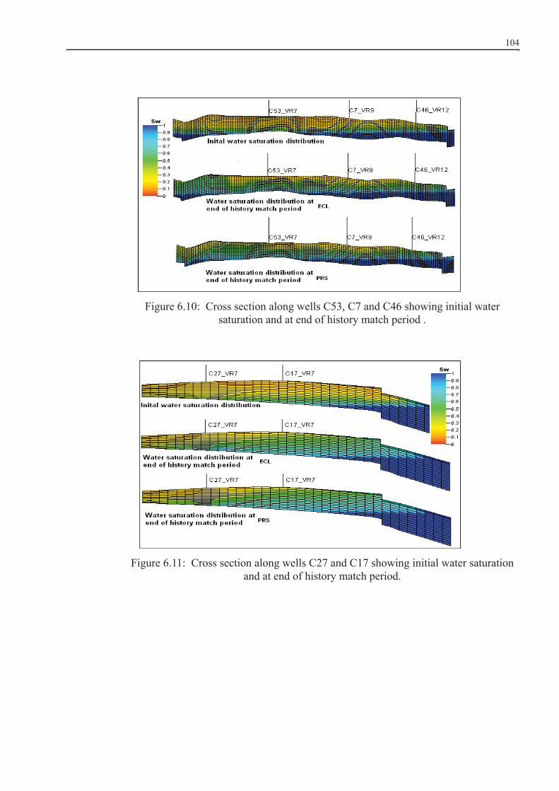
104
Figure 6.10: Cross section along wells C53, C7 and C46 showing initial water saturation and at end of history match period .
Figure 6.11: Cross section along wells C27 and C17 showing initial water saturation and at end of history match period.

105
Chapter 7
Closing Remarks
The author strongly believes that the objectives formulated in Chapter 1 were fullyachieved. The original idea was proved as workable and the TPPM workflow could beestablished and improved step by step. The code became robust with the time andgenerally usable. The method was already applied to the fields
1. Maros, gas reservoir, UGS, Hungary, operated by E’ON, 2008.2. AHM, oil field, Libya, operated by Akakus, 20093. North Gialo and Farigh, oil field, operated by WAHA
4. Libba, oil field, operated by Harouge, 2009.
The last three fields together have an OOIP of over 30 Bstb. The author sees an enormouspotential to apply TPPM in Libya. Most of the reservoirs contain undersaturated oil andare depleted by bottom water drive, similar to the example field.
TPPM was developed in PRS but it could be easily implemented in any other simulationsoftware, especially in ECLIPSE. Such a step would help to make it available for theentire petroleum producing industry.
It is sure that there is a large potential for further developments. TPPM has a certain kindof artificial intelligence capability. TPPM fails if there is not enough oil, water and gas ata certain spot in the model at a given time to satisfy the historical target production. Insuch situations the simulator can estimate the reasons for the failure, and can suggestpossible improvements in the geological model. Such developments were alreadyinitiated. PRS offers also some auxiliary methods as material balance and displacementcalculation, decline curve analysis, well test capability, single well modeling, etc. whichcan be used in combination with TPPM.
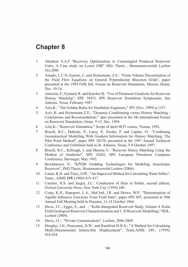
106
Chapter 8
1 Abrahem S.A.F "Recovery Optimization in Commingled Produced ReservoirUnits, A Case study on Lower GIR" MSc Thesis , Montanuniversität LeobenOct.2006
2 Amado, L.C.N, Ganzer, L. and Heinemann, Z.E.: "Finite Volume Discretization ofthe Fluid Flow Equations on General Perpendicular Bisection Grids", paperpresented at the 1994 Fifth Intl. Forum on Reservoir Simulation, Muscat, Oman,Dec. 10-14.
3 Anterion, F., Eymard, R. and Karcher B.: "Use of Parameter Gradients for ReservoirHistory Matching", SPE 18433, SPE Reservoir Simulation Symposium, SanAntonio, Texas, February 1987.
4 Aziz,K.: "Ten Golden Rules for Similation Engineers," JPT (Nov. 1989) p.1157.5 Aziz, K. and Heinemann Z.E.: "Dynamic Conditioning versus History Matching -
Conclusions and Recomandations." aper presented at the 5th International Forumon Reservoir Simulation, Oman 9-13. Dec. 1994.
6 Aziz,K.: "Reservoir Simulation," Script of short HOT course, Vienna, 1992.7 Bissell, R.C., Dubrule, P., Lamy, P., Swaby, P. and Lepine, O.: "Combining
Geostatisctical Modelling With Gradient Information for History Matching: ThePilot Point Method", paper SPE 38370, presented at the 1997 Annual TechnicalConference and Exhibition held in St. Antonio, Texas, 5-8 October 1997.
8 Bissell, R.C., Killough, J. and Sharma Y.: "Resevoir Histoy Matching Using theMethod of Gradients", SPE 24265, SPE European Petroleum ComputerConference, Stavanger, May 1992.
9 Brockhauser, S.: "KPEBI Gridding Technologies for Modeling AnisotropicReservoir", PhD Thesis, Montanuniversität Leoben (2004).
10 Carter, R.D. and Tracy, G.W.: "An Improved Method for Calculating Water Influx",Trans., AIME 219, (1960) 415-417.
11 Carslaw, H.S. and Jaeger, J.C.: Conduction of Heat in Solids, second edition,Oxford University Press, New York City (1959) 100.
12 Coats, K.H., Rapoport, L.A., McCord, J.R. and Drews, W.P.: "Determination ofAquifer Influence Functions From Field Data", paper SPE 897, presented at 39thAnnual Fall Meeting held in Houston, 11-14 October 1964.
13 Davis, J.C., Egger, S., and : "Kotla Intergrated Reservoir Study, Volume 4. KotlaField Geological Reservoir Characteraization and 3_D Reservoir Modelling," HOL,Leoben (2009).
14 Davis, J.C.: "Private Comunications", Leoben, 2006-2009.15 Douglas, J.Jr., Peacemen, D.W.: and Rachford H.H.Jr.: "A Method for Calculating
Multi-Dimensuoinal Immiscible Displecement", Trans.AIME 249., (1959),418-424.
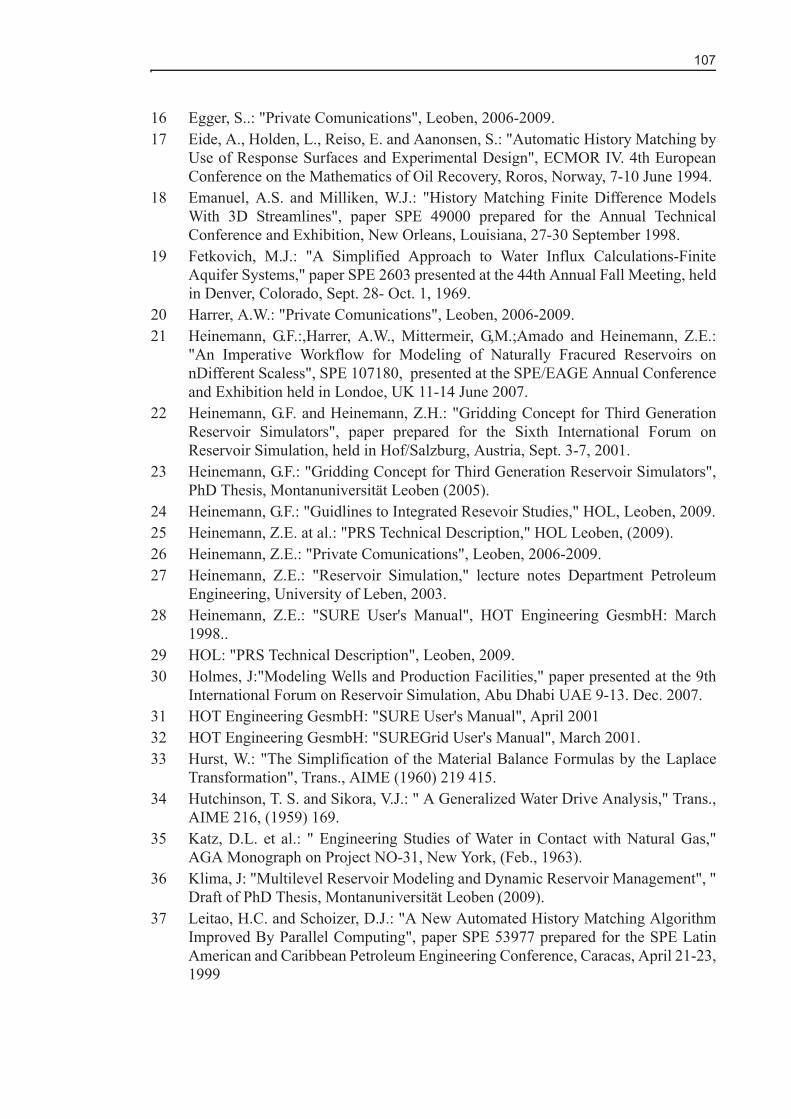
107
16 Egger, S..: "Private Comunications", Leoben, 2006-2009.17 Eide, A., Holden, L., Reiso, E. and Aanonsen, S.: "Automatic History Matching by
Use of Response Surfaces and Experimental Design", ECMOR IV. 4th EuropeanConference on the Mathematics of Oil Recovery, Roros, Norway, 7-10 June 1994.
18 Emanuel, A.S. and Milliken, W.J.: "History Matching Finite Difference ModelsWith 3D Streamlines", paper SPE 49000 prepared for the Annual TechnicalConference and Exhibition, New Orleans, Louisiana, 27-30 September 1998.
19 Fetkovich, M.J.: "A Simplified Approach to Water Influx Calculations-FiniteAquifer Systems," paper SPE 2603 presented at the 44th Annual Fall Meeting, heldin Denver, Colorado, Sept. 28- Oct. 1, 1969.
20 Harrer, A.W.: "Private Comunications", Leoben, 2006-2009.21 Heinemann, G.F.:,Harrer, A.W., Mittermeir, G,M.;Amado and Heinemann, Z.E.:
"An Imperative Workflow for Modeling of Naturally Fracured Reservoirs onnDifferent Scaless", SPE 107180, presented at the SPE/EAGE Annual Conferenceand Exhibition held in Londoe, UK 11-14 June 2007.
22 Heinemann, G.F. and Heinemann, Z.H.: "Gridding Concept for Third GenerationReservoir Simulators", paper prepared for the Sixth International Forum onReservoir Simulation, held in Hof/Salzburg, Austria, Sept. 3-7, 2001.
23 Heinemann, G.F.: "Gridding Concept for Third Generation Reservoir Simulators",PhD Thesis, Montanuniversität Leoben (2005).
24 Heinemann, G.F.: "Guidlines to Integrated Resevoir Studies," HOL, Leoben, 2009.25 Heinemann, Z.E. at al.: "PRS Technical Description," HOL Leoben, (2009).26 Heinemann, Z.E.: "Private Comunications", Leoben, 2006-2009.27 Heinemann, Z.E.: "Reservoir Simulation," lecture notes Department Petroleum
Engineering, University of Leben, 2003.28 Heinemann, Z.E.: "SURE User's Manual", HOT Engineering GesmbH: March
1998..29 HOL: "PRS Technical Description", Leoben, 2009.30 Holmes, J:"Modeling Wells and Production Facilities," paper presented at the 9th
International Forum on Reservoir Simulation, Abu Dhabi UAE 9-13. Dec. 2007.31 HOT Engineering GesmbH: "SURE User's Manual", April 200132 HOT Engineering GesmbH: "SUREGrid User's Manual", March 2001.33 Hurst, W.: "The Simplification of the Material Balance Formulas by the Laplace
Transformation", Trans., AIME (1960) 219 415.34 Hutchinson, T. S. and Sikora, V.J.: " A Generalized Water Drive Analysis," Trans.,
AIME 216, (1959) 169.35 Katz, D.L. et al.: " Engineering Studies of Water in Contact with Natural Gas,"
AGA Monograph on Project NO-31, New York, (Feb., 1963).36 Klima, J: "Multilevel Reservoir Modeling and Dynamic Reservoir Management", "
Draft of PhD Thesis, Montanuniversität Leoben (2009). 37 Leitao, H.C. and Schoizer, D.J.: "A New Automated History Matching Algorithm
Improved By Parallel Computing", paper SPE 53977 prepared for the SPE LatinAmerican and Caribbean Petroleum Engineering Conference, Caracas, April 21-23,1999

108
38 Le Ravalec-Dupin, M. and Fenwick, D.H.: "A combined Geostatistical andStreamline Based History Matching Procedue," paper SPE 77378 prepared for theSPE Anual Technical Conference and Exhibition held in San Antonio, Texas, 29Sep- 2 Oct 2002.
39 MacMillan, D.J., Pletcher, J.L. and Bourgeois, S.A.: "Practical Tools To AssistHistory Matching", paper SPE 51888, prepared for the SPE Reservoir SimulationSymposium held in Houston, Texas, 14-17 February 1999.
40 Menissi, M.H., Kenawy, F.A., Mohamed, S.A. and Sallaly, M.E.El.: "DevelopmentOf Aquifer Influence Function for Undersaturated Oil Reservoir UsingSemi-Analytical Model, " paper SPE 39747, presented at the 1998 SPE Asia PacificConference on Integrated Modelling for Asset Management held in Kula Lumpur,Malaysia, 23-24 March 1998.
41 Mittermeir, G.M.R. at al.: "Kotla Intergrated Reservoir Study", Volume 1-7. HOL,Leoben (2009).
42 Mittermeir, G.M.R., Pichelbauer,J. and Heinemann, Z.E.: "AutomathedDetermination of Aquifer Properties from Fiel Production Data, paper presented atthe 9th European Conference on Mathematics of Oil Recovery (ECMOR IX),Cannes, France, Aug.30-Sep.2, 2004.
43 Mittermeir, G.M.R.: "Performance Prediction of Natulally Fractured ReservoirsUsing Simulation Models on Different Scales", PhD Thesis, MontanuniversitätLeoben (2006).
44 Mittermeir, G.M.R.:"Enhanced Strategies for Matching Aquifer Behaviour", MSThesis, Montanuniversität Leoben (2003).
45 Mittermeir, G.M.R.:"Private Comunications", Leoben, 2006-2009.46 Mlacnik, M.J.: "Using Well Windows in Full Field Reservoir Simulation", PhD
Thesis, Montanuniversität Leoben (2002)47 Modine, A.D., Coats, K.H. and Wells, M.W.: "A supperposition Method for
Representing Wellbore Crossflow in Reservoir Simulation", SPE ReservoirEngineering, Vol.7. No.3. Aug.1992.
48 Numbere, D.T.: "Natural Water Influx in Nonsymmetric Reservoir/AquiferSystems", paper SPE 19850 prepared for the 64th Annual Technical Conferenceand Exhibition held in San Antonio, Texas, 8 - 11 October 1989.
49 Ouenes, A., Bhagavan, S., Bunge, P.H. and Travis B.J.: "Application of SimulatedAnnealing and Other Global Optimisation Methods to Reservoir Description",paper SPE 28415, presented at the 69th Annual Conference and Exhibition held inNew Orleans, 25-28 September 1994.
50 Peacemen, D.W.: ""Interpretation of Well-Block Pressures in Numerical ReservoirSimulation", Soc.Petr.Eng.Jour, 18, (1978), 183-194: Trans.AIME 265, (1978).
51 Pichelbauer, J.: "New Methor of Aquifer Matching in Reservoir Simulation",.PhDThesis, Montanuniversität Leoben (2003).
52 Portella, R.C.M. and Prais, F.: "Use of Automatic History Matching andGeostatistical Simulation to Improve Production Forecast," paper SPE 53976presented at the 1999 SPE Latin American and Caribbean Petroleum EngineeringConference held in Caracas, Venezuela, 21-23 April 1999.
53 Roggero, F. and Hu, L.-Y.: "Gradual deformation of continuous geostatistical

109
models for history matching", paper SPE 49004 prepared for the Annual TechnicalConference and Exhibition, New Orleans, Louisiana, 27-30 September 1998.
54 Sarma, P., Durlofsky, L.J., Aziz, K. and Chen, W.H.: !A new Approach toAutomatic History Matching Using Kernel PCA," paper SPE 106176 MS,presented at the sPE Reservoir Simulation Symposium, 26-28 February 2007,Houston, Texas USA.
55 Schilthuis, R.J.: "Active Oil and Reservoir Energy", Trans., AIME 118, (1936)33-52.
56 Schiozer, D.J.: "User Of Reservoir Simulation, Parallel Computing andOptimization Techniques to Accelerate History Matching and ReservoirManagement Decisions", pater SPE 53979 prepared for the SPE Latin Americanand Caribbean Petroleum Engineering Conference, Caracas, April 21-23, 1999
57 Schulze-Riegert, R. and Ghedan G.Sh.:"Modern Techniques for History Matching,"paper presented at the 9th International Forum on Reservoir Simulation, Abu DhabiUAE 9-13. Dec. 2007.
58 Schlumberger: Eclipse 100 manual, 2008A.59 Tan, T.B. and Kalgerakis, N.: "A Fully Implicit, Three Dimensional, Three Phase
Simulator with Automatic History Matching Capability", SPE 21205, SPEReservoir Simulation Symposium, Anaheim, Ca, February 17-20 1991.
60 Tan, T.B. and Kalgerakis, N.: "Improved Reservoir Characterisation UsingAutomatic History Matching Procedures", JCPT, June 1993, Vol 32, No. 6, 26-32.
61 Tracy, G.W.: "Simplified Form of the Material Balance Equation", Trans., AIME204, (1955) 243-248.
62 VanEverdingen, A.F. and Hurst, W.: "The Application of the LaplaceTransformation to Flow Problems in Reservoirs", Trans., AIME 186, (1949)305-324.
63 VanEverdingen, A.F. and Hurst, W.: "Water Influx into a Reservoir and ItsApplication to the Equation of Volumetric Balance", Trans., AIME 151, (1943)57-72.
64 Vogt, J.P. and Wang, B.: "Accurate Formulas for Calculating the Water InfluxSuperposition Integral", paper SPE 17066 presented at the 1987 SPE EasternRegional Meeting held in Pittsburgh, Pennsylvania, 21-23 October 1987.
65 Williams, M.A., Keating, J.F. and Barghouty, M.F.: " The Stratigraphic Method: AStructured Approach to History Matching Complex Simulation Models", paper SPE38014 presented at the 1997 SPE Reservoir Simulation Symposium held in Dallas,8-11 June 1997.

110
Chapter 9
Nomenclature
SymbolsA - area, cross section, [m²]
cp - compressibility factor of phase p [1/bar]
ct - total compressibility factor [1/bar]
c - apparent pore compressibility factor [1/bar]
Dp - specific mole density, [kmol/m³]
Dpc - diffusion coefficient, [m²/s]
- gravity acceleration vector, [m/s²]
- molar flux of component c in phase p, [kmol/m² s]
- permeability tensor
k - permeability, [m²]
krp - relative permeability, [-]
Mc - molar mass of component c, [kg/mol]
- normal unit vector
N - total number of grid cells
OOIP - original oil in place [m³]
pp - phase pressure, [bar]
ptarget - target pressure, [bar]
qp - flow rate of phase p, [m³/s]
qp - source/sink term for phase p, [kmol/day]
qcmf - matrix-fracture transfer term, [kmol/day]
Sp - phase saturation, [-]
g
Jpc
k
n

111
t - time [days]
T - temperature, [K]
- filtration velocity, [m/day]
VI - Volume of gridblock I, [m²]
Vp - Pore volume, [m³]
V - Pore volume, [m³]
Vp1 - Volume of phase p produced during phase p’ imbibition, [m³]
Vp2 - Volume of phase p produced during phase p’ flooding, [m³]
VT - Bulk volume, [m³]
xpc - mole fraction of component c in phase p, [-]
z - depth, [m]
Greek Symbols- porosity, [-]
p - phase potential, [bar]
p - phase mobility, [1/cp]
p - phase viscosity, [cp]
p - phase density, [kg/m³]
IJ - interblock transmissibility, [m³]
- time difference operator,
- boundary
Subscripts
c - component
g - gas
i - initial conditions
i - shape factor class
i - point index
ir - irreducible
k - location on the recovery curve
k+1 - location on the recovery curve
up
t tn 1+ n–=

112
l - left
m - matrix
n - old time level
n+1 - new time level
o - oil
p - phase
r - relative
r - residual
r - right
w - water
x,y,z - coordinate directions
Superscripts
Nc - total number of components
Np - total number of phases
- old iteration level
+1 - new iteration level
Conversion Factors
bar = psia*0.06894757
m = ft*0.3048
kg = lb*0.453592
1000m3 = MMSCF*26.795
kg/m3 = lb/ft3*16.01846
°F = °R-459.67
°C =
°API =
F-321.8
------------------141.5
Spec. Gravity-131.5------------------------------------------------

113
Appendix C
C.1 Results of Well by Well Matching for the Full Field Project
The full field example is described in Chapter 4 and Chapter 6. It is not possible toincorporate all results of the history matching in this work but this supplement shouldprovide an insight into the amount of the study work and its excellent results. TheAppendix C exists in two versions, this second one is the neutralized and reduced version.
Corresponding to the TPPM workflow the target rates for the wells would be defined as3 phase rate, as wet rate and in the end phase as net oil rate. Therefore the oil rate is alwayscorrect equal to the historical values. The history matching can be qualified on the basesof the cumulative water production and the water rate and the water cut respectively. Theclassifications are excellent, good, fair and failed. The respective limits are given in theTable C.1
Table C.1: Limits applied to assess the quality of the history match
• Excellent: if all differences are considerably under the limits;• Good: The differences are below the limits; • Fair: The differences are above the limit but the tendencies are similar. The
simulation result gives the possibility of a quantitative estimation of futureperformance;
• Failed: The real and model wells behave differently.
The result of the history matching is summeriesd in Table C.2 to Table C.4. The Figure
C.1 to Figure C.21show examples for the 4 categories.
%Cum. oil production 1%Cum. water production 5%Cum. liquid production 5%Difference in oil production rate at the end of HM: 1%
Difference in water production rate at end of HM:10% excellent, 20% good,50% acceptable, 50 bbl abs. excellent
Difference in water breakthrough time less than 6 monthMax. difference in WC at the end of HM 5%Static bottomhole pressure noneDynamic BHP Not compared

114
C.1.1 Tabulated Results:
Table C.2: Full Field Example Summary of Well by Well Match Part1.
Well VR
Cum.Oil
Prod.
Avg.Oil
Prod.Rate
End HM
Qualityof
match
Qualityof
matchQualityover all
Start End Historical Historical Cum. Rate Both[-] [-] [Date] [Date] [Mstb] [stb/day] [-] [-] [-]
C43 VR2 1982 1991 128 0 Good GoodC44 VR2 1985 Act. 969 64 Good Excell. GoodC49 VR2 1985 1994 165 0 Fair FairC36 VR3 1993 Act. 697 124.2 Excell. Excell. Excell.C45 VR3 2003 Act. 524 263.5 Good Good Good C33 VR4 1980 Act. 5560 131.3 Fair Fair Fair C35 VR4 1985 2008 2157 0 Fair Fair C37 VR4 1985 Act. 5996 508.1 Excell. Excell. Excell.C39 VR4 1981 2007 1542 0 Fair Fair C42 VR4 1982 Act. 1942 31.3 Excell. Good GoodC58H VR4 2002 Act. 1275 344.5 Fair Good Fair C34 VR4 1988 1989 17 0 Failed Failed C52 VR4 1992 Act. 4256 325.1 Good Good GoodC10 VR5 1965 1992 1675 0 Excell. Excell.C40 VR5 1987 1994 303 0 Excell. Excell.C32 VR5 1980 1999 4263 0 Good GoodC38 VR5 1985 Act. 3894 194.8 Excell. Excell. Excell.C62 VR6 2006 Act. 272 135.5 Good Excell. GoodC17 VR7 1965 1995 1572 0 Good GoodC31 VR7 1979 Act. 14482 598.6 Good Excell. GoodC25 VR7 1978 Act. 5835 126.5 Excell. Excell. Excell.C27 VR7 1978 Act. 6840 208.5 Excell. Excell. Excell.C29 VR7 1978 1991 1028 0 Good GoodC30 VR7 1979 Act. 5564 437 Excell. Good GoodC41 VR7 1982 Act. 1995 81 Good Good GoodC53 VR7 1982 Act. 1094 104.7 Excell. Good Excell.
Production

115
Table C.3: Full Field Example Summary of Well by Well Match Part2.
Table C.4: Summary of Full Field Example History Match Quality Classification on Well Basis
Well VR
Cum.Oil
Prod.
Avg.Oil
Prod.Rate
End HM
Qualityof
match
Qualityof
matchQualityover all
Start End Historical Historical Cum. Rate Both[-] [-] [Date] [Date] [Mstb] [stb/day] [-] [-] [-]
C19 VR17 1965 1992 9739 0 Excell. Excell.C24 VR17 1977 Act. 6809 415.2 Excell. Excell. Excell.C26 VR17 1978 Act. 6788 333.2 Excell. Excell. Excell.C28 VR17 1978 Act. 2756 149.3 Good Good Good C18 VR17 1965 Act. 8986 141.7 Excell. Excell. Excell.C51 VR17 1992 Act. 2903 365.9 Excell. Excell. Excell.C56 VR17 1993 Act. 2788 407.1 Excell. Excell. Excell.C57H VR17 2001 Act. 2225 747.4 Good Excell. Good C59H VR7 2002 Act. 1589 531.3 Excell. Excell. Excell.C6 VR17 1964 1991 12028 0 Excell. Excell.C22 VR8 1970 1977 233 0 Fair FairC8 VR8 1964 Act. 11107 166.8 Excell. Excell. Excell.C21 VR9 1970 Act. 5671 200.9 Good Good GoodC23 VR9 1977 2000 3369 0 Excell. Excell.C3 VR9 1965 1977 1019 0 Excell. Excell.C54 VR9 1993 Act. 2798 293.4 Excell. Excell. Excell.C55 VR9 1993 Act. 1264 258.8 Good Excell. GoodC7 VR9 1964 1977 4382 0 Good GoodC2 VR12 1965 1968 563 0 Excell. Excell.C16 VR12 1965 1972 184 0 Good GoodC46 VR12 1986 Act. 661 78.7 Good Excell. GoodC48 VR12 1987 Act. 1928 148.8 Excell. Excell. Excell.C50 VR12 1992 2009 822 13.7 Excell. Excell. Excell.C66 VR12 2009 Act. 82 390 Fair Failed Failed
Production
Full Field Example
Classification
CategoryCum. Production(50 wells total)
CategoryRate End of HM(50 wells total)
CategoryOverall Quality(50 wells total)
Excellent 50% 69% 46%Good 34% 28% 38%Fair 14% 0% 12%
Failed 25% 3% 4%
History Match Quality Classification

116
C.1.2 Examples for Excellent HM:
Figure C.1 C38_VR5 Oil rate in history matching period.
Figure C.2 C38_VR5 Water Cut

117
Figure C.3 C38_VR5 Cumulative oil production
Figure C.4 C48_VR12 Oil rate in history matching period

118
Figure C.5 C48_VR12 Water Cut
Figure C.6 C48_VR12 Cumulative oil production
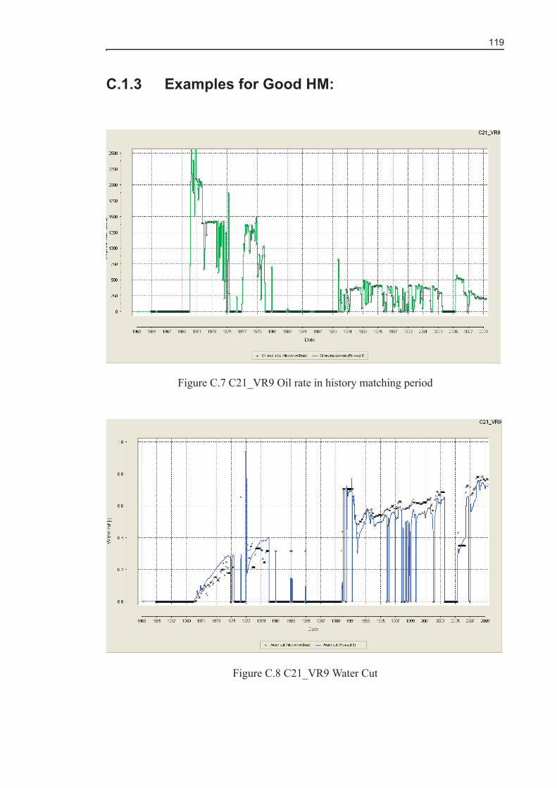
119
C.1.3 Examples for Good HM:
Figure C.7 C21_VR9 Oil rate in history matching period
Figure C.8 C21_VR9 Water Cut

120
Figure C.9 C21_VR9 Cumulative oil production
Figure C.10 C24_VR17 Oil rate in history matching period

121
Figure C.11 C24_VR17 Water Cut
Figure C.12 C24_VR17 Cumulative oil production
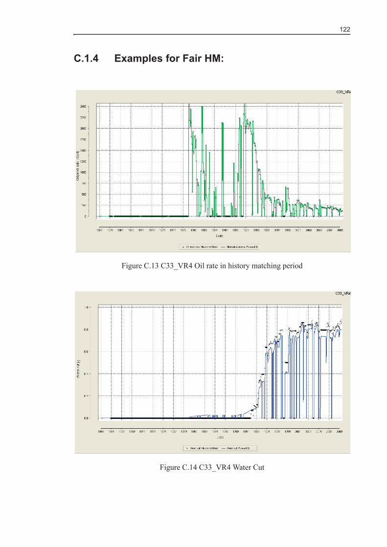
122
C.1.4 Examples for Fair HM:
Figure C.13 C33_VR4 Oil rate in history matching period
Figure C.14 C33_VR4 Water Cut

123
Figure C.15 C33_VR4 Cumulative oil production
Figure C.16 C58H_VR4 Oil rate in history matching period

124
Figure C.17 C58H_VR4 Water Cut
Figure C.18 C58H_VR4 Cumulative oil production

125
C.1.5 Examples for failed plots:
Figure C.19 C34_VR4 Oil rate in history matching period
Figure C.20 C34_VR4 Water Cut

126
Figure C.21 C34_VR4 Cumulative oil production