a new 1km digital elevation model of the antarctic derived ...a new 1km digital elevation model of...

The Cryosphere, 3, 101–111, 2009www.the-cryosphere.net/3/101/2009/© Author(s) 2009. This work is distributed underthe Creative Commons Attribution 3.0 License.

The Cryosphere

A new 1 km digital elevation model of the Antarctic derived fromcombined satellite radar and laser data – Part 1: Data and methods

J. L. Bamber1,2, J. L. Gomez-Dans1,*, and J. A. Griggs2

1Centre for Polar Observations and Modelling, School of Geographical Sciences, University of Bristol, UK2Bristol Glaciology Centre, School of Geographical Sciences, University of Bristol, UK* now at: Environmental Monitoring Group, Department of Geography, King’s College London, UKand Remote Sensing Unit, Department of Geography, University College London, UK

Received: 18 September 2008 – Published in The Cryosphere Discuss.: 25 November 2008Revised: 2 April 2009 – Accepted: 2 April 2009 – Published: 4 May 2009

Abstract. Digital elevation models (DEMs) of the wholeof Antarctica have been derived, previously, from satelliteradar altimetry (SRA) and limited terrestrial data. Near theice sheet margins and in other areas of steep relief the SRAdata tend to have relatively poor coverage and accuracy. Toremedy this and to extend the coverage beyond the latitudinallimit of the SRA missions (81.5◦ S) we have combined laseraltimeter measurements from the Geosciences Laser Altime-ter System onboard ICESat with SRA data from the geode-tic phase of the ERS-1 satellite mission. The former pro-vide decimetre vertical accuracy but with poor spatial cover-age. The latter have excellent spatial coverage but a poorervertical accuracy. By combining the radar and laser datausing an optimal approach we have maximised the verticalaccuracy and spatial resolution of the DEM and minimisedthe number of grid cells with an interpolated elevation esti-mate. We assessed the optimum resolution for producing aDEM based on a trade-off between resolution and interpo-lated cells, which was found to be 1 km. This resulted injust under 32% of grid cells having an interpolated value.The accuracy of the final DEM was assessed using a suiteof independent airborne altimeter data and used to producean error map. The RMS error in the new DEM was foundto be roughly half that of the best previous 5 km resolu-tion, SRA-derived DEM, with marked improvements in thesteeper marginal and mountainous areas and between 81.5and 86◦ S. The DEM contains a wealth of information relatedto ice flow. This is particularly apparent for the two largestice shelves – the Filchner-Ronne and Ross – where the sur-face expression of flow of ice streams and outlet glaciers can

Correspondence to:J. L. Bamber([email protected])

be traced from the grounding line to the calving front. Thesurface expression of subglacial lakes and other basal fea-tures are also illustrated. We also use the DEM to derive newestimates of balance velocities and ice divide locations.

1 Introduction

Surface topography is an important data set for a wide rangeof applications from fieldwork planning to numerical mod-elling studies. It can, for example, be used to validate theability of a model to reproduce the present-day geometry ofthe ice sheet or as an input boundary condition for mod-elling or combined with other data to estimate steady-statevelocities and ice thickness (Bamber et al., 2000; Budd andWarner, 1996; Warner and Budd, 2000). Estimates of themass balance of Antarctica using a mass budget approach arecritically dependent on accurate surface topography for esti-mating i) drainage basin areas and ii) ice thickness close tothe grounding line (Joughin and Bamber, 2005; Rignot andThomas, 2002; Rignot et al., 2008) as direct measurements ofice thickness are sparse. A recent study of the accuracy of ex-isting, published DEMs of Antarctica, found that large errors(in excess of hundreds of metres) were ubiquitous in areas ofhigher surface slope such as near the margins of the ice sheet,in mountainous terrain such as the Transantarctic Mountainsand also beyond the latitudinal limit of satellite radar altime-ter measurements (Bamber and Gomez-Dans, 2005).

An ICESat-only DEM has been produced (DiMarzio etal., 2008) with reasonable accuracy where data exist (Younget al., 2008) but, as explained below, the across-track spac-ing is too coarse to provide adequate coverage for latitudesless than about 80◦ S. In addition to this, a number of high

Published by Copernicus Publications on behalf of the European Geosciences Union.

http://creativecommons.org/licenses/by/3.0/

102 J. L. Bamber et al.: A new Antarctic digital elevation model: data and methods

accuracy regional DEMs have been produced from a combi-nation of terrestrial and/or satellite data sets (e.g. Fricker etal., 2000; Wesche et al., 2007). In general, these have beenlimited to specific sectors such as the Amery ice shelf, for ex-ample (Fricker et al., 2000). In a related paper we use someof the terrestrial data, employed in these studies, as a valida-tion of the DEM presented here (Griggs and Bamber, 2008).New regional topographic data sets are being developed forthe marginal areas of Antarctica from SPOT 5 stereoscopicdata (Korona et al., 2009), and photoclinometry based onMODIS imagery, is being used to increase the spatial res-olution of this and other DEMs (Haran et al., 2008). Furtherinto the future, significant improvements in both spatial reso-lution and accuracy, particularly around the margins, shouldbe afforded by satellite missions such as TanDEM-X – a twinsatellite interferometric synthetic aperture radar mission –and CryoSat 2, both slated for launch in late 2009. Data fromthese missions should be available by late 2010/early 2011.

As a consequence of the limitations in the existingcontinental-scale DEMs and the availability of a source ofhigh accuracy elevation data for many of the areas that are“problematic” for SRAs, we have produced a new DEMof the Antarctic continent. We have combined the high-accuracy, but relatively low spatial resolution, laser altime-ter measurements from the Geoscience Laser Altimeter Sys-tem, GLAS, onboard the ICESat satellite, with radar altime-ter data from the geodetic phase of the ERS-1 satellite, whichprovide high spatial sampling but lower vertical accuracy.The result is a DEM, where the number of interpolated gridpoints has been minimised while improving the accuracy ofthe topography for areas of high relief and south of 81.5◦ Slatitude. Stereo-photogrammetric and cartographic data havenot been used in this study although they could improve theaccuracy in high-relief regions such as the TransantarcticMountains (Liu et al., 1999, updated 2001).

2 Data sets and processing

In March 1994 ERS-1 was placed in two long repeat cyclesof 168 days. The two phases were offset from each otherso that they were equivalent to a single 336 day cycle, pro-viding 8.3 km across-track spacing at the equator. This re-duces to about 4 km at 60◦ S latitude and 2 km at 70◦ S. Thealong-track spacing of each altimeter height measurement is335 m and the footprint size is∼4 km. The total numberof data points, after filtering, over the ice sheet was about40 million (Bamber and Bindschadler, 1997). The data re-duction methodology has been described, in detail, elsewhere(Bamber, 1994) and this is the same data set that was used toproduce an earlier 5 km posting DEM of Antarctica (Bamberand Bindschadler, 1997).

We have combined the ERS-1 data with all the available,reliable ICESat data, as listed in Table 1. ICESat has an alongtrack spacing of 170 m and an across-track spacing of about

Table 1. Operation periods of ICESat data used in current DEM.

Laser Start Date End Date

1a 20/02/2003 21/03/20032a 25/09/2003 18/11/20032b 17/02/2004 21/03/20042c 18/05/2004 21/06/20043a 03/10/2004 08/11/20043b 17/02/2005 24/03/20053c 20/05/2005 23/06/20053d 21/10/2005 24/11/20053e 22/02/2006 28/03/20063f 24/05/2006 26/06/20063g 25/10/2006 27/11/20063h 12/03/2007 14/04/20073i 02/10/2007 05/11/20073j 17/02/2008 21/03/2008

Table 2. Amount of ICESat data removed by each stage of the QAfiltering.

Filter No of datapoints Percentage remaining

Original data 144632388After geophysical filters 122328755 84.6%After 3 sigma filter 121728068 84.2%After DEM filter 115619957 79.9%

20 km at 70◦ S. In contrast to the radar altimeter, the foot-print size of ICESat was∼70 m. The data product used herewas the level 2 Antarctic and Greenland Ice Sheet AltimetryData product (GLA12) and all data used were release version428 (Zwally et al., 2007). The data were extracted using thesoftware provided by the National Snow and Ice Data center(NSIDC) and transformed from the Topex/Poseidon ellipsoidto the WGS84 ellipsoid for consistency with the ERS-1 dataand the geoid model applied. Corrections were also appliedto account for saturation of the laser over the ice sheet asrecommended by the NSIDC.

Geophysical quality assurance filters were used to removethose returns which may contain residual cloud or other arte-facts that affect the elevation estimate. The geophysical fil-ters used were:

1. Attitude control classified as good

2. Only 1 waveform detected

3. Reflectivity of surface greater than 10%

4. Gain less than 200

5. Variance of waveform from Gaussian less than 0.03 V

These filters combined, removed 5.4% of the data (Table 2).

The Cryosphere, 3, 101–111, 2009 www.the-cryosphere.net/3/101/2009/

J. L. Bamber et al.: A new Antarctic digital elevation model: data and methods 103

The data were gridded with 5 km spacing and a 3 standarddeviation filter was applied to remove additional elevationoutliers. Visual inspection indicated that a small number ofanomalous ERS and ICESat data remained and these wereremoved in a final filtering step. This was achieved by usinga preliminary version of the 1 km DEM (Bamber and Gomez-Dans, 2005) and removing points where the difference was>(11.5× slope angle) for slopes between 0.1 and 1◦. Thesevalues were chosen based on the standard deviation of differ-ences between ICESat and ERS data as a function of surfaceslope derived in an earlier study (Bamber and Gomez-Dans,2005). Data were only filtered in this step if they originatefrom an area where the surface slope was less 1◦. In areasof higher slope, individual returns may be expected to havelarge departures from the average surface height in the gridbox and so such a filter is inappropriate. Also at these highersurface slopes, there are relatively few data points in the com-parison between ICESat and ERS. Surface slopes were de-termined with a 2 km spatial resolution from the “first guess”DEM. This final quality assurance filter removed a further4% of the original data. An ICESat roughness filter, used inthe earlier study (Bamber and Gomez-Dans, 2005) was notapplied here. This filter used a roughness estimate derivedfrom the ICESat waveforms. The most recent data releasesno longer contain this variable due to errors in the way it wascalculated. The pattern of surface slopes over the ice sheet,as determined from the final DEM, is shown in Fig. 1 to indi-cate the regions affected by this filter and the range of surfaceslopes over the continent.

2.1 ERS data pre-processing

The ERS data used are the same as those used to derivea 5 km Antarctic DEM in the 1990s (Bamber and Bind-schadler, 1997). The data have been retracked, slope-corrected and filtered, as described elsewhere (Bamber,1994; Bamber and Bindschadler, 1997). These data wereshown to suffer a roughness-dependent surface bias, whichwas believed to be due to the fact that the SRA does notsample kilometre scale surface roughness uniformly (Bam-ber, 1994; Bamber et al., 1998; Bamber and Gomez-Dans,2005). Instead the peaks of undulations are oversampledcompared to the troughs, causing a positive bias in the ob-served elevations, which increases with the amplitude of theundulations. The bias was removed by calculating the dif-ference between the ERS-1 and ICESat data as a functionof surface roughness over a length scale of 5 km. Surfaceroughness was determined from the standard deviation of thesurface slope of a “first guess” DEM for a 5×5 grid centredon the cell in question. The bias, calculated as a functionof roughness, binned with 0.01◦ intervals is shown in Fig. 2.Up to a roughness of∼0.15◦, there is a near-linear increasein bias from zero to 16 m. Beyond this point the relation-ship breaks down. At roughness values above 0.25◦, boththe bias and standard deviation of the bias estimate decrease

491 492

493

494

Fig 1. Surface slopes, estimated from the new DEM over a 2 km length scale. The limit of

satellite altimeter coverage is indicated by the green circle at 86º S.

Page 19

Fig. 1. Surface slopes, estimated from the new DEM over a 2 kmlength scale. The limit of satellite altimeter coverage is indicated bythe green circle at 86◦ S.

with increasing roughness (Fig. 2). There is no physical ex-planation for this behaviour and the number of points used tocalculate the bias is relatively small at these higher roughnessvalues. In addition, only 4% of the ice sheet has a roughnessexceeding 0.25◦ (Fig. 2b), representing the steepest and mosttopographic areas such as the Transantarctic mountains. As aconsequence, we do not apply a correction for these areas, asno physically-based bias can be determined. The maximumbias correction is, therefore, 16 m (Fig. 2a). Figure 3 showsthe spatial pattern of the correction applied to the ERS databased on the relationship shown in Fig. 2 up to a roughnessof 0.25◦. The unshaded areas over the ice sheet in Fig. 3 areregions where the roughness either exceeded 0.25◦ or whereno ERS data were present. This is generally in areas of highrelief where the increased roughness and the variable surfacegradients caused the ERS-1 radar altimeter to lose lock ofthe surface return. It should be noted that the roughness es-timate described above correlates closely with regional sur-face slope (Fig. 1) except in areas where the second deriva-tive of the surface (i.e. curvature) is small, such as on the icerises and islands on the Ross and Filchner Ronne ice shelves(see inset in Fig. 3). These areas are “smooth” over kilome-tre length-scales while possessing a non-negligible regionalslope (Fig. 1). It was largely for this reason that, here, wedetermined the bias as a function of roughness (Griggs andBamber, 2008) as opposed to surface slope as was done inearlier studies (Bamber et al., 1998; Bamber and Gomez-Dans, 2005).

www.the-cryosphere.net/3/101/2009/ The Cryosphere, 3, 101–111, 2009


495 496

497

498

499

500

Figure 2 a) Plot of the mean difference (ICESat-ERS-1) between the ICESat and ERS-1 data over

Antarctica as a function of surface roughness. The inset shows the first part of the graph, up to

0.25º, for which a bias correction was applied. Figure b) Standard deviation of the mean

difference shown in figure a (solid line) and cumulative percentage ice sheet area as a function of

surface roughness (dashed line).

Page 20

Fig. 2. (a) Plot of the mean difference (ICESat-ERS-1) betweenthe ICESat and ERS-1 data over Antarctica as a function of surfaceroughness. The inset shows the first part of the graph, up to 0.25◦,for which a bias correction was applied.(b) Standard deviation ofthe mean difference shown in figure a (solid line) and cumulativepercentage ice sheet area as a function of surface roughness (dashedline).

2.2 Time stamp and data weighting

The ERS data are not contemporaneous with the ICESat ob-servations and so a correction for surface elevation changesbetween the acquisition period of the ERS data (1994–1995)and the ICESat data (2003–2008) was applied. Here, we usedannual elevation change estimates derived from ERS radaraltimetry between 1992 and 2003 (Davis et al., 2005). A cor-rection was only applied in regions where the height changeover the entire period was more than 1m as this was assumedto be the likely cumulative error in the measurements basedon an∼10 cm/yr detection limit. In addition, no correctionwas applied to the ice shelves.

A number of previous studies have shown that the RMSerror of SRA over the ice sheets degrades with increasing re-

501

502 503

504

505

506

Figure 3. Spatial distribution of the roughness-bias correction, between 0 and 10 m, applied to the

ERS-1 data. The inset shows Berkner Island and surrounding shelf ice. The unshaded areas over

the continent are mainly areas where no ERS-1 data were present.

Page 21

Fig. 3. Spatial distribution of the roughness-bias correction, be-tween 0 and 10 m, applied to the ERS-1 data. The inset showsBerkner Island and surrounding shelf ice.

gional slope (Bamber et al., 1998; Bamber and Gomez-Dans,2005; Brenner et al., 2007). The SRA data were, therefore,weighted according to an estimate of their accuracy as a func-tion of surface slope. The weights were calculated using theequation below, which was derived from a degree-two poly-nomial fit to the standard deviation of the difference betweenICESat and ERS data as a function of surface slope. TheRMS difference between the fit and the data was also 0.47 m.

weight =

{ 2.352552.35255+19.3115∗slope+16.1766∗slope2

for slope angles< 1◦

150 for slope angles≤ 1◦

2.3 Choice of DEM resolution

An optimal DEM resolution is desirable, which is a trade-off between minimizing the number of interpolated points,while maximising the spatial detail in the original data. Themetric used to determine the optimum resolution here wasthe ratio between the number of grid cells containing obser-vations against those that did not (i.e. grid cells where thevalue is interpolated). For convenience, we have called thisthe interpolation ratio. The coverage of the two altimetersused in this study is latitude dependent, increasing toward thelatitudinal limit of the satellite orbits of 81.5◦ and 86◦ S forERS-1 and ICESat respectively (Fig. 4). We examined theinterpolation ratio for three latitudinal bands: 70–75, 75–80and 80–85◦ S. The first band is largely populated, numeri-cally, by ERS data, the middle band is a mixture of the twowhile the last band is dominated by ICESat data. The num-ber of observations, however, does not necessarily reflect the



70o

80o

0 10

500 km 600 km

a)

b) c)

Fig. 4. Number of satellite observations between 0 and 10 in each1 km grid cell. (a) covers the whole continent. The red boxes indi-cated the areas shown in (b) and (c).(b) shows a section of the RossIce Shelf including the Siple Coast and Roosevelt Island;(c) showsthe Amery ice shelf and surrounding grounded ice sheet region.

“importance” of ERS data compared to ICESat because, inareas of higher slope in particular, the ERS data may be heav-ily down-weighted. Thus, for example, where the slope isgreater than 1◦, 50 SRA observations have the same weightas a single ICESat observation. Nonetheless, Fig. 4 illus-trates some important points about the variability in spatialsampling by ERS and ICESat, as a function of latitude andsurface slope. The white bands at∼81 and∼86◦ S indicatethe latitudinal limits of the two satellites, where coverage isdense and spatial sampling high. The light-coloured linescrossing the continent indicate ICESat tracks where, locally,the sampling is high because we have used multiple repeattracks. Between these lines are areas of blue to green and yel-low, which reflect grid cells where only ERS data are present.This can be more clearly seen in Fig. 4b and c. The latter (theAmery Ice Shelf) covers an area relatively far north at around70◦ S where the across track spacing of ICESat is evidently

513 514

515

516

Figure 5: Percentage of interpolated cells as a function of cell size and latitude for combined ERS

and ICESat data.

Page 23

Fig. 5. Percentage of interpolated cells as a function of cell size andlatitude for combined ERS and ICESat data.

coarse and where the majority of the grid cells are populatedby ERS data only. In the area just upstream of the ground-ing line of the ice shelf is a band of black, where no dataare present, most probably due to the high relief in this areaand the filters applied to the ERS data described earlier. Thedense coverage provided by ERS-1 over the two largest iceshelves is illustrated in Fig. 4b and is due to the low reliefand proximity to the latitudinal limit of the satellite. Figure 4demonstrates the importance of the ERS-1 data for providingobservations between the ICESat tracks, particularly for lati-tudes north of about 80◦ S, where the across-track spacing ofICESat is around 15 km.

The interpolation ratios were calculated using the numberof valid data points within each latitude band, which werebinned into cells with spacings between 500 and 5000 m.Figure 5 shows the results of this analysis. For a cell size of1 km, the percentage of interpolated points (i.e. those whereno satellite data fall within the grid cell) is between 20 and40% depending on the latitude band. At resolutions smallerthan this, the percentage rapidly increases. We believe, there-fore, that a DEM with 1 km postings provides a realistic rep-resentation of the true resolution of the input data at the con-tinental scale. Using this value, resulted in 31.8% of gridcells having an interpolated value or, put another way, 68%of grid cells contained measured elevation estimates. A vari-able resolution DEM or regional models at higher resolutioncould be considered, particularly in areas close to latitudes of81.5 and 86◦ S.

2.4 Data gridding and interpolation

Data were first re-sampled onto a quasi-regular 1 km grid bycalculating the mean x, y and z values for each cluster ofsatellite data falling within a grid cell. The mean z estimateswere weighted values of the combined ERS and ICESat data.The weights for ICESat data were 1.0 and for the ERS data



were inversely proportional to the variance of the differencebetween ERS and ICESat as a function of surface slope, asdiscussed earlier. A land/ocean mask was applied to thequasi regular grid so that data over ocean/sea ice were not in-cluded in the interpolation and did not create biases at the iceedge. The mask defining the coastline was created using ver-sion 5 of the Antarctic Digital Database (ADDconsortium,2006) which has a variable resolution of between 5 m andgreater than 5 km. The data were then interpolated onto aregular 1 km polar stereographic grid with a standard paral-lel of 71◦ S, using ordinary kriging using open source soft-ware GSLIB (Deutsch and Journel, 1997). The variogramwas estimated from data from the quasi regular grid witha balance velocity (see Sect. 3), greater than 50 m/yr. Thiswas done to because the slow-moving interior has low vari-ance and high data density. In this region the interpolationis relatively insensitive to the chosen variogram but it is thelargest region by area and would, therefore, dominate the var-iogram properties if included. The Peninsula was excluded asit is non representative of the statistical properties elsewhere.The variogram was modelled as a Gaussian function fit to thefirst 10 km of lag. The fit parameters were range = 25 763 mand sill = 1005 m. A nugget of 1 m was also included. Themaximum search radius for including data in the interpola-tion was chosen as 50 km and the maximum number of datapoints that could contribute to an interpolated value was 50.In data sparse and mountainous regions (along the Antarc-tic Peninsula and Transantarctic Mountains) a handful ofclearly erroneous interpolated values were identified from vi-sual inspection of DEM surface slope values. These pointswere replaced using a nearest neighbour approach. South of86◦ S, ADD cartographic data were merged with the DEMby weighting the two datasets using Hermite basis functionsover a distance of 40 km at the southern limit of the satellitedataset.

2.5 Ocean tide correction for the ice shelves

Ocean tide corrections were removed from both the ERS-1and ICESat data and replaced with a tide model, TPXO6.2(Egbert and Erofeeva, 2002), that has been determined to bean optimum model for the entire circum-Antarctic seas (Kingand Padman, 2005). All tidal components (8 major and 16minor) were applied using the grounding line mask that camewith the model. In some areas of floating ice we are awarethat the mask lies seaward of the true grounding line, whichwill reduce the precision of the elevations in these small ar-eas. The ocean loading and solid earth tides provided withthe ERS and ICESat products were used to correct for thesetwo effects.

517 518

519

520

521

Figure 6. Planimetric shaded relief plot of the 1 km digital elevation model. Ice divides, derived

from the DEM, are shown in red; the green circle marks the limit of satellite altimeter coverage;

the two blue boxes indicate the areas plotted in greater detail in Figures 7 and 9.

Page 24

Fig. 6. Planimetric shaded relief plot of the 1 km digital eleva-tion model. Ice divides, derived from the DEM, are shown inred; the green circle marks the limit of satellite altimeter coverage;the two blue boxes indicate the areas plotted in greater detail inFigs. 7 and 9.

3 Results

The complete DEM is shown in Fig. 6 and illustrates thelarge-scale topographic features such as ice divides, the iceshelves and the region lacking satellite coverage south of alatitude of 86◦ S. Also shown are the location of ice dividesobtained from the DEM and used in a mass budget study ofthe ice sheet to separate flow between drainage basins (Rig-not et al., 2008).

It is not possible to see the full resolution and detailedtopography at a continental scale. Figure 7 illustrates thefiner-scale (both horizontal and vertical) topography presentin the DEM for the Filchner-Ronne Ice Shelf. The redline indicates the location of the grounding line as obtainedfrom the MODIS mosaic of Antarctica (Haran et al., 2006).There is good agreement between this and the limit of float-ing ice based on the break in slope as identified from theDEM. Flow stripes, traceable from the grounding line to icefront are clearly visible and are associated with ice streamflow into the ice shelf and around grounded “obstacles” suchas Berkner Island. Their amplitude varies between around50 cm and 3 m and they have a width of a few kilometres,which is clearly resolved in the DEM (Fig. 8). Not sur-prisingly, the ICESat-only DEM (DiMarzio et al., 2008), al-though gridded at 500 m spacing, does not capture all theflow-stripes, due to the relatively sparse across-track spac-ing of the satellite (c.f. Fig. 4). The surface expression of



522 523

524

525

526

527

Figure 7. Shaded relief plot of the Filchner Ronne Ice Shelf and surrounding grounded ice sheet.

The grounding line for the ice shelf, from the MODIS mosaic of Antarctica (Haran et al., 2006),

is shown in red. The location of the elevation profile plotted in Figure 8 is shown by the green

line.

Page 25

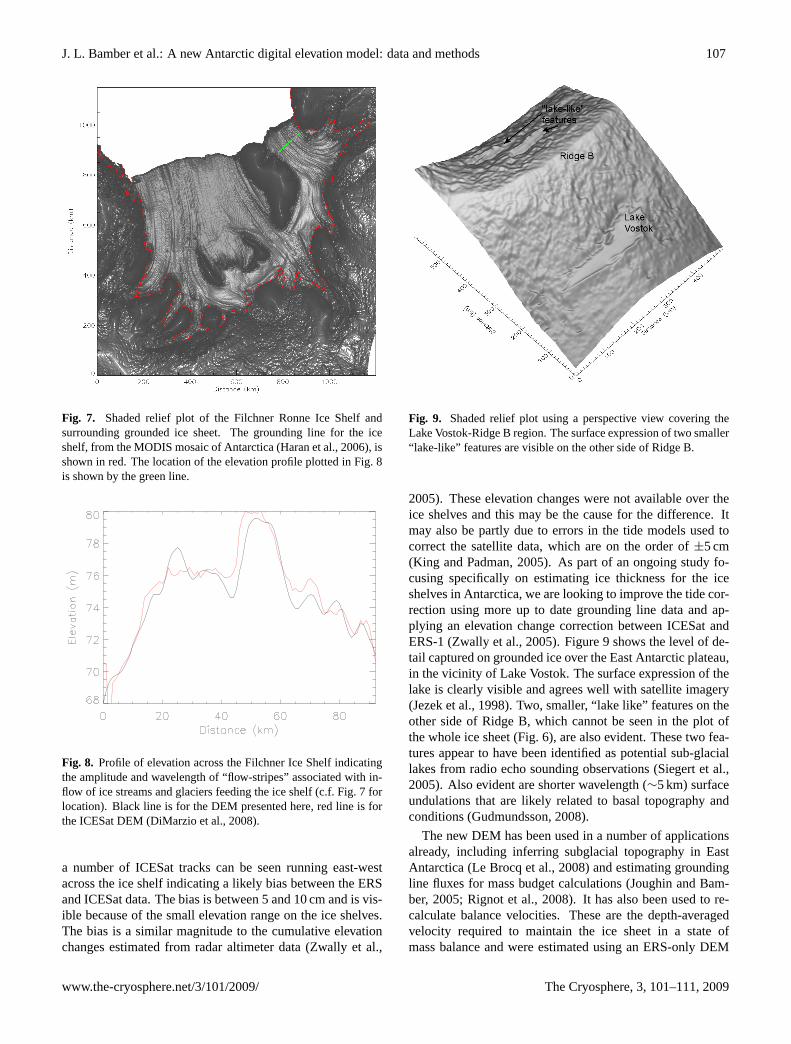
Fig. 7. Shaded relief plot of the Filchner Ronne Ice Shelf andsurrounding grounded ice sheet. The grounding line for the iceshelf, from the MODIS mosaic of Antarctica (Haran et al., 2006), isshown in red. The location of the elevation profile plotted in Fig. 8is shown by the green line.

Fig. 8. Profile of elevation across the Filchner Ice Shelf indicatingthe amplitude and wavelength of “flow-stripes” associated with in-flow of ice streams and glaciers feeding the ice shelf (c.f. Fig. 7 forlocation). Black line is for the DEM presented here, red line is forthe ICESat DEM (DiMarzio et al., 2008).

a number of ICESat tracks can be seen running east-westacross the ice shelf indicating a likely bias between the ERSand ICESat data. The bias is between 5 and 10 cm and is vis-ible because of the small elevation range on the ice shelves.The bias is a similar magnitude to the cumulative elevationchanges estimated from radar altimeter data (Zwally et al.,

534 535

536

537

538

Figure 9. Shaded relief plot using a perspective view covering the Lake Vostok-Ridge B region.

The surface expression of two smaller “lake-like” features are visible on the other side of Ridge

B.

Page 27

Fig. 9. Shaded relief plot using a perspective view covering theLake Vostok-Ridge B region. The surface expression of two smaller“lake-like” features are visible on the other side of Ridge B.

2005). These elevation changes were not available over theice shelves and this may be the cause for the difference. Itmay also be partly due to errors in the tide models used tocorrect the satellite data, which are on the order of±5 cm(King and Padman, 2005). As part of an ongoing study fo-cusing specifically on estimating ice thickness for the iceshelves in Antarctica, we are looking to improve the tide cor-rection using more up to date grounding line data and ap-plying an elevation change correction between ICESat andERS-1 (Zwally et al., 2005). Figure 9 shows the level of de-tail captured on grounded ice over the East Antarctic plateau,in the vicinity of Lake Vostok. The surface expression of thelake is clearly visible and agrees well with satellite imagery(Jezek et al., 1998). Two, smaller, “lake like” features on theother side of Ridge B, which cannot be seen in the plot ofthe whole ice sheet (Fig. 6), are also evident. These two fea-tures appear to have been identified as potential sub-glaciallakes from radio echo sounding observations (Siegert et al.,2005). Also evident are shorter wavelength (∼5 km) surfaceundulations that are likely related to basal topography andconditions (Gudmundsson, 2008).

The new DEM has been used in a number of applicationsalready, including inferring subglacial topography in EastAntarctica (Le Brocq et al., 2008) and estimating groundingline fluxes for mass budget calculations (Joughin and Bam-ber, 2005; Rignot et al., 2008). It has also been used to re-calculate balance velocities. These are the depth-averagedvelocity required to maintain the ice sheet in a state ofmass balance and were estimated using an ERS-only DEM



539 540

541

542

543

544

545

546

Figure 10. Balance velocities for Antarctica, calculated at 5 km spacing using the new digital

elevation model, accumulation rates from the output of a regional climate model (Van de Berg et

al., 2006) and the BEDMAP ice thickness compilation (Lythe and Vaughan, 2001) supplemented

with new thickness data for the Amundsen Sea Sector (Holt et al., 2006). The green circle marks

the limit of satellite altimeter data used in earlier DEMs of Antarctica. The blue circle marks the

limit in this study.

Page 28

Fig. 10. Balance velocities for Antarctica, calculated at 5 km spac-ing using the new digital elevation model, accumulation rates fromthe output of a regional climate model (Van de Berg et al., 2006) andthe BEDMAP ice thickness compilation (Lythe and Vaughan, 2001)supplemented with new thickness data for the Amundsen Sea Sec-tor (Holt et al., 2006). The green circle marks the limit of satellitealtimeter data used in earlier DEMs of Antarctica. The blue circlemarks the limit in this study.

previously (Budd and Warner, 1996). Here, we have com-bined the new DEM with the BEDMAP ice thickness dataset (Lythe and Vaughan, 2001) and surface mass balance datafrom the output of a regional climate model (Van de Berg etal., 2006). The result is shown in Fig. 10. The most sig-nificant differences in the spatial pattern of balance veloc-ities compared to the previous result (Bamber et al., 2000)is for the region between 81.5 and 86◦ S. In particular theglaciers feeding the Ross Ice Shelf through the Transantarc-tic mountains and the ice streams along the Siple Coast havea somewhat different “structure”. Differences here and fur-ther north, such as along the Amundsen Sea sector and feed-ing Getz Ice Shelf are also due to significant differences inthe spatial pattern of accumulation produced by the regionalclimate model compared with the observationally-based dataset used in the earlier analysis (van de Berg et al., 2005).

To investigate the impact of the new DEM on the delin-eation of ice divides we have compared those derived fromthe older, 5 km DEM derived from ERS-1 data, which wereused in a reassessment of the mass balance of Antarctica(Vaughan et al., 1999) with those derived from the new DEMand used for a similar purpose (Rignot et al., 2008). Thecomparison is shown in Fig. 11. Not surprisingly, the agree-ment is good for the low-slope Antarctic plateau region up

547 548

549

550

551

552

Figure 11. Drainage basins estimated from an older radar altimeter DEM of Antarctica, in black,

(Vaughan et al., 1999) compared with basins identified using the new 1 km DEM (Rignot et al.,

2008) shown in red. The two coloured circles are as for figure 10. The catchments feeding

Support Force and Foundation Ice Stream are indicated by SUP and FOU, respectively.

Page 29

Fig. 11. Drainage basins estimated from an older radar altimeterDEM of Antarctica, in black, (Vaughan et al., 1999) compared withbasins identified using the new 1 km DEM (Rignot et al., 2008)shown in red. The two coloured circles are as for Fig. 10. Thecatchments feeding Support Force and Foundation Ice Stream areindicated by SUP and FOU, respectively.

to the latitudinal limit of ERS-1 (green circle). Between thisand the limit of ICESat (blue circle) there are differences inbasin area as well as in the fidelity of the delineation process.The red ice divides (using the new DEM) separate the catch-ments for each ice stream feeding the Filchner Ronne andRoss ice shelves. This was not possible, within acceptableerrors, with the earlier DEMs that did not incorporate ICE-Sat data (Bamber and Bindschadler, 1997; Liu et al., 1999,updated 2001). South of the blue circle, at 86◦ S there re-mains uncertainty over the catchment areas for Foundationand Support Force glacier based on, essentially the same ter-restrial data.

3.1 Validation and error analysis

A suite of independent airborne elevation measurements havebeen used to assess the accuracy of the DEM as a function ofsurface slope, roughness and other parameters. These datawere also used to produce an error map and the details aredescribed in a companion paper (Griggs and Bamber, 2008).We summarize, therefore, the key points only. In compari-son to the best (the one with the lowest RMS errors) of thetwo previously published DEMs derived primarily from SRAdata (Bamber and Bindschadler, 1997; Liu et al., 1999) theRMS error has been reduced by about a factor two (Griggsand Bamber, 2008). The RMS differences are also less thana DEM derived solely from ICESat data (DiMarzio et al.,



2008) but only by around 5–32% depending on the area con-sidered. Uniquely for Antarctica, an error map has been de-rived based on the results of the validation analysis and astepwise regression against the variables believed to be cor-related with errors in the DEM.

4 Discussion

In an earlier study, ICESat data were used to assess theaccuracy of two current DEMs of Antarctica (Bamber andGomez-Dans, 2005). The accuracy was determined as afunction of surface slope. One was found to have a monoton-ically increasing bias with slope with a value of around 10 mfor a slope of 1◦. The standard deviation for this DEM was∼45 m at the same angle and around 68 m for the other DEM.Comparison with a suite of independent validation data indi-cates that the random error in our new DEM is around halfthat of the “better” of the two models assessed previouslyand that the bias is close to zero for all slopes (Griggs andBamber, 2008). Between 81.5 and 86◦ S the improvement isgreater still as the earlier DEMs were reliant on sparse, pooraccuracy terrestrial data. The accuracy of topography in thisregion, prior to the launch of ICESat, was nearer±100 m(Bamber and Gomez-Dans, 2005). Not surprisingly, there-fore, balance velocities estimated using our new DEM differsignificantly in terms of spatial pattern compared with an ear-lier estimate. The accuracy of the DEM south of 86◦ S stillremains an issue with no immediate solution evident. Bal-ance velocities, and other variables sensitive to slope, such asice divides, will continue to have a higher uncertainty southof 86◦ S. Crucially, however, the satellite observations nowcover the entirety of the grounding lines of all the ice shelves(Figs. 1 and 10). These data can, and have been used, there-fore, to determine ice thickness close to the grounding lineassuming hydrostatic equilibrium and taking account of firndensity variations (Helsen et al., 2008; Rignot et al., 2008).As part of this work, elevations from the DEM along thegrounding line of Ice Stream D were compared with airbornelidar data with an accuracy of<40 cm (Blankenship et al.,2001). The mean difference in elevation along the ground-ing line was 0.15 m±4.0 m. This implies a bias of around1 m in ice thickness and random error of 35 m equivalent to∼ 5%. Figure 3 indicates that the bias in the ERS-1 data issmall (5–10 cm) over the ice shelves but increases markedlyinland of the grounding line. The difference (ICESat-ERS) isnegative, indicating that the ERS-1 data are biased high. Notaccounting for this bias could, therefore, result in an over-estimation of ice thickness close to the grounding line. Ad-ditionally, it is evident that ICESat data alone are inadequatefor determining grounding line elevations for all except thoselying south of about 80◦ S (Fig. 4). Figure 12 shows the cov-erage of ICESat tracks in greater detail over the Amery IceShelf, which lies at about 70◦ S. The lighter (whiter) linesindicate the ICESat tracks. There are about fifteen cover-

Page 30

553 554

555

556

Figure 12. Number of satellite observations between 0 and 15 in each 1 km grid cell for the

Lambert Glacier region and Amery Ice Shelf.

Fig. 12. Number of satellite observations between 0 and 15 in each1 km grid cell for the Lambert Glacier region and Amery Ice Shelf.

ing the entirety of the grounding line (shown in red) whilethe blue-green colours indicate ERS-1 data, which providealmost complete coverage at the grid spacing of 1 km usedhere. Inland of the grounding line is an∼20 km wide bandshaded black, where the ERS-1 data are absent due to thesteep relief and the filtering steps, described earlier, appliedto the data.

5 Conclusions

We present a new digital elevation model of Antarctica withgrid spacing of 1 km, chosen to balance the proportion ofgrid cells that contained an interpolated value while max-imising the spatial resolution of the DEM. We undertook acareful and comprehensive filtering of both data sets usinga range of geophysical and instrument-based tests to ensurethat the effect of clouds, off-ranging and other artefacts wereeliminated. An extensive suite of independent airborne laserand radar altimeter measurements was used to undertake athorough analysis of the accuracy of the DEM. These datawere also used to produce an error map (Griggs and Bam-ber, 2008). Random errors were found to be predominantlya function of surface slope and roughness, ranging between∼50 cm and 20 m for the RMS error and typical range ofslopes/roughness over the ice sheet. This roughly halves therandom error compared to an earlier DEM without the bene-fit of ICESat data (Bamber and Gomez-Dans, 2005). For theregion between 81.5 and 86◦ S, the improvement in accuracyand resolution is larger still and has a marked effect on thespatial pattern of balance velocities and drainage basins de-rived using the new DEM. Both the DEM and error map willbe made available through the National Snow and Ice DataCenter for long-term archival.



Acknowledgements.This work was funded by UK NERC contractfor the Centre for Polar Observations and Modelling and NERCgrant NE/E004032/1. We would like to thank Helen Fricker andfour anonymous referees for their comments and improvements tothe paper.

Edited by: S. Dery

References

Antarctic digital database, 2006.Bamber, J. L.: Ice sheet altimeter processing scheme, Int. J. Rem.

Sens., 14, 925–938, 1994.Bamber, J. L. and Bindschadler, R. A.: An improved elevation data

set for climate and ice sheet modelling: Validation with satelliteimagery, Ann. Glaciol., 25, 439–444, 1997.

Bamber, J. L., Ekholm, S., and Krabill, W. B.: The accuracy ofsatellite radar altimeter data over the greenland ice sheet deter-mined from airborne laser data, Geophys. Res. Lett., 25, 3177–3180, 1998.

Bamber, J. L., Vaughan, D. G., and Joughin, I.: Widespread com-plex flow in the interior of the antarctic ice sheet, Science, 287,1248–1250, 2000.

Bamber, J. L. and Gomez-Dans, J. L.: The accuracy of digital el-evation models of the antarctic continent, Earth Plan. Sci. Lett.,217, 516–523, 2005.

Blankenship, D. D., Morse, D. L., Finn, C. A., Bell, R. E., Peters,M. E., Kempf, S. D., Hodge, S. M., Studinger, M., Behrendt,J. C., and Brozena, J. M.: Geological controls on the initiationof rapid basal motion for the west antarctic ice streams: A geo-physical perspective including new airborne radar sounding andlaser altimetry results, in: The west antarctic ice sheet: Behaviorand environment, edited by: Alley, R. B. and Bindschadler, R.,American Geophysical Union, Washington DC, 105–122, 2001.

Brenner, A. C., DiMarzio, J. R., and Zwally, H. J.: Precision andaccuracy of satellite radar and laser altimeter data over the con-tinental ice sheets, IEEE T. Geosci. Rem. Sens., 45, 321–331,2007.

Budd, W. F. and Warner, R. C.: A computer scheme for rapid cal-culations of balance-flux distributions, Ann. Glaciol., 23, 21–27,1996.

Davis, C. H., Li, Y., McConnell, J. R., Frey, M. M., andHanna, E.: Snowfall-driven growth in east antarctic ice sheetmitigates recent sea-level rise, Science, 308, 1898–1901,doi:10.1126/1110662, 2005.

DiMarzio, J., Brenner, A. C., Schutz, R., Shuman, C. A., andZwally, H. J.: Glas/icesat 500 m laser altimetry digital elevationmodel of antarctica, 2008, National Snow and Ice Data Center,2008.

Deutsch, C. L. and Journel, A. G.: Gslib. Geostatistical softwarelibrary and user’s guide, Second ed., Oxford University Press,Oxford, 369 pp., 1997.

Egbert, G. D. and Erofeeva, S. Y.: Efficient inverse modeling ofbarotropic ocean tides, J. Atmos. Oceanic Technol., 19, 183–204,2002.

Fricker, H. A., Hyland, G., Coleman, R., and Young, N. W.: Digitalelevation models for the lambert glacier-amery ice shelf system,east antarctica, from ers-1 satellite radar altimetry, J. Glaciol., 46,553–560, 2000.

Griggs, J. A. and Bamber, J. L.: A new 1 km digital elevation modelof Antarctica derived from combined radar and laser data – Part2: Validation and error estimates, The Cryosphere, 3, 113–123,2009,http://www.the-cryosphere-discuss.net/3/113/2009/.

Gudmundsson, G. H.: Analytical solutions for the surface responseto small amplitude perturbations in boundary data in the shallow-ice-stream approximation, The Cryosphere, 2, 77–93, 2008,http://www.the-cryosphere-discuss.net/2/77/2008/.

Haran, T. M., Scambos, T. A., Fahnestock, M. A., and Csatho, B.M.: New enhancements of an ers1-2 + icesat digital elevationmodel of west antarctica using modis imagery, shapelets, andkriging, Eos Trans. AGU, 89, Abstract C31A-0461, 2008.

Helsen, M. M., van den Broeke, M. R., van de Wal, R. S. W.,van de Berg, W. J., van Meijgaard, E., Davis, C. H., Li, Y.,and Goodwin, I.: Elevation changes in antarctica mainly de-termined by accumulation variability, Science, 320, 1626–1629,doi:10.1126/science.1153894, 2008.

Holt, J. W., Blankenship, D. D., Morse, D. L., Young, D. A.,Peters, M. E., Kempf, S. D., Richter, T. G., Vaughan, D. G.,and Corr, H. F. J.: New boundary conditions for the westantarctic ice sheet: Subglacial topography of the thwaites andsmith glacier catchments, Geophys. Res. Lett., 33, L09502,doi:10.1029/2005GL025561, 2006.

Jezek, K. C., Sohn, H. G., and Noltimier, K. F.: The radarsat antarc-tic mapping project, 1998 International Geoscience and RemoteSensing Symposium (IGARSS 98) on Sensing and Managing theEnvironment, SEATTLE, WA, 6–10 Jul 1998, 2462–2464, 1998.

Joughin, I. and Bamber, J. L.: Thickening of the ice stream catch-ments feeding the filchner-ronne ice shelf, antarctica, Geophys.Res. Lett., 32, L17503, doi:10.1029/2005GL023844, 2005.

King, M. A. and Padman, L.: Accuracy assessment of ocean tidemodels around antarctica, Geophys. Res. Lett., 32, L23608,doi:10.1029/2005GL023901, 2005.

Korona, J., Berthier, E., Bernard, M., Remy, F., and Thou-venot, E.: Spirit. Spot 5 stereoscopic survey of polar ice:Reference images and topographies during the fourth in-ternational polar year (2007–2009), J. Photogramm., 64,doi:10.1016/j.rse.2008.1009.1015, 204–212, 2009.

Le Brocq, A. M., Hubbard, A., Bentley, M. J., and Bam-ber, J. L.: Subglacial topography inferred from ice surfaceterrain analysis reveals a large un-surveyed basin below sealevel in east antarctica, Geophys. Res. Lett., 35, L16503,doi:10.1029/2008GL034728, 2008.

Liu, H. X., Jezek, K. C., and Li, B. Y.: Development of an antarcticdigital elevation model by integrating cartographic and remotelysensed data: A geographic information system based approach,J. Geophys. Res.-Solid Earth, 104, 23199–23213, 1999.

Lythe, M. B. and Vaughan, D. G.: Bedmap: A new ice thickness andsubglacial topographic model of antarctica, J. Geophys. Res.-Solid Earth, 106, 11335-11351, 2001.

Rignot, E. and Thomas, R. H.: Mass balance of polar ice sheets,Science, 297, 1502–1506, 2002.

Rignot, E., Bamber, J. L., van den Broeke, M. R., Davis, C., Li, Y.,van de Berg, W. J., and van Meijgaard, E.: Recent antarctic icemass loss from radar interferometry and regional climate mod-elling, Nature Geosci., 1, 106–110, doi:10.1038/ngeo102, 2008.

Siegert, M. J., Carter, S., Tabacco, I., Popov, S., and Blankenship,D. D.: A revised inventory of antarctic subglacial lakes, Antarct.


http://www.the-cryosphere-discuss.net/3/113/2009/

http://www.the-cryosphere-discuss.net/2/77/2008/


Sci., 17, 453–460, doi:10.1017/s0954102005002889, 2005.van de Berg, W. J., van den Broeke, M., and Reijmer, C. H.: Charac-

teristics of the antarctic surface mass balance (1958–2002) usinga regional atmospheric climate model, Ann. Glaciol., 41, 97–104,2005.

Van de Berg, W. J., van den Broeke, M. R., van Meijgaard,E., and Reijmer, C. H.: Reassessment of the antarctic sur-face mass balance using calibrated output of a regional at-mospheric climate model, J. Geophys. Res., 111, D11104,doi:10.1029/2005JD006495, 2006.

Vaughan, D. G., Bamber, J. L., Giovinetto, M., Russell, J., andCooper, A. P. R.: Reassessment of net surface mass balance inantarctica, J. Climate, 12, 933–946, 1999.

Warner, R. C. and Budd, W. F.: Derivation of ice thickness andbedrock topography in data-gap regions over antarctica, Ann.Glaciol., 31, 191–197, 2000.

Wesche, C., Eisen, O., Oerter, H., Schulte, D., and Steinhage, D.:Surface topography and ice flow in the vicinity of the edml deep-drilling site, antarctica, J. Glaciol., 53, 442–448, 2007.

Young, D. A., Kempf, S. D., Blankenship, D. D., Holt, J. W., andMorse, D. L.: New airborne laser altimetry over the thwaitesglacier catchment, west antarctica, Geochem. Geophys. Geosys.,9, Q06006, doi:10.1029/2007GC001935, 2008.

Zwally, H. J., Giovinetto, M. B., Li, J., Cornejo, H. G., Beckley, M.A., Brenner, A. C., Saba, J. L., and Donghui, Y.: Mass changesof the greenland and antarctic ice sheets and shelves and contri-butions to sea-level rise: 1992–2002, J. Glaciol., 51, 509–527,2005.


a new 1km digital elevation model of the antarctic derived ...a new 1km digital elevation model of...

Documents