a neural network approach using multi-scale textural metrics from very high-resolution panchromatic...

Remote Sensing of Environment 113 (2009) 1276–1292

Contents lists available at ScienceDirect

Remote Sensing of Environment

j ourna l homepage: www.e lsev ie r.com/ locate / rse

A neural network approach using multi-scale textural metrics from veryhigh-resolution panchromatic imagery for urban land-use classification

Fabio Pacifici a,⁎, Marco Chini b, William J. Emery c

a Earth Observation Laboratory, Tor Vergata University, Rome, Italyb Istituto Nazionale di Geofisica e Vulcanologia, Rome, Italyc Colorado University, Boulder, Colorado, USA

⁎ Corresponding author.E-mail address: [email protected] (F. Pacific

0034-4257/$ – see front matter © 2009 Elsevier Inc. Adoi:10.1016/j.rse.2009.02.014

a b s t r a c t
a r t i c l e i n f o
Article history:Received 31 July 2008Received in revised form 13 February 2009Accepted 14 February 2009

Keywords:Extended pruningMulti-scale textural analysisNeural networksQuickBirdUrban land-useVery high-resolution panchromatic dataWorldView-1

The successful launch of panchromatic WorldView-1 and the planned launch of WorldView-2 will make amajor contribution towards the advancement of the commercial remote sensing industry by providingimproved capabilities, more frequent revisits and greater imaging flexibility with respect to the precursorQuickBird satellite. Remote sensing data from panchromatic systems have a potential for more detailed andaccurate mapping of the urban environment with details of sub-meter ground resolution, but at the sametime, they present additional complexities for information mining.In this study, very high-resolution panchromatic images from QuickBird and WorldView-1 have been used toaccurately classify the land-use of four different urban environments: Las Vegas (U.S.A.), Rome (Italy),Washington D.C. (U.S.A.) and San Francisco (U.S.A.). The proposed method is based on the analysis of first-and second-order multi-scale textural features extracted from panchromatic data. For this purpose, texturalparameters have been systematically investigated by computing the features over five different windowsizes, three different directions and two different cell shifts for a total of 191 input features. Neural NetworkPruning and saliency measurements made it possible to determine the most important textural features forsub-metric spatial resolution imagery of urban scenes.The results show that with a multi-scale approach it is possible to discriminate different asphalt surfaces,such as roads, highways and parking lots due to the different textural information content. This approach alsomakes it possible to differentiate building architectures, sizes and heights, such as residential houses,apartment blocks and towers with classification accuracies above 0.90 in terms of Kappa coefficientcomputed over more than a million independent validation pixels.

© 2009 Elsevier Inc. All rights reserved.

1. Introduction

Human activity truly dominates the Earth's ecosystems withstructural modifications. Rapid population growth over recent decadesand the concentration of this population in and aroundurban areas havesignificantly impacted the environment (Pacifici et al., 2007). Althoughurban areas represent a small fraction of the land surface, they affectlarge areas due to the magnitude of the associated energy, food, waterand raw material demands. Urban areas are undergoing dynamicchanges and, as a consequence, are facingnewspatial andorganizationalchallenges as they seek to manage local urban development within aglobal community. Sub-urbanization refers to a highly dynamic processwhere rural areas, both close to, but also distant from, city centersbecome enveloped by, or transformed into, extended metropolitanregions. These areas are a key interface between urban and rural areasdue to the provision of essential services in both (GLP, 2005).

i).

ll rights reserved.

During the last two decades, significant progress has been made indeveloping and launching satellites with instruments, in both theoptical/IR and microwave regions of the spectra, well suited for Earthobservation with an increasingly finer spatial and spectral resolutions(Bamler and Eineder, 2008; ESA, 2006; DigitalGlobe, 2008a; Digital-Globe, 2008b). The successful launch of WorldView-1 in September2007 and the planned launch of WorldView-2 have made and willmake a major contribution towards the advancement of thecommercial remote sensing industry by providing greater capability,more frequent revisits and greater imaging flexibility with respect tothe precursor QuickBird satellite. WorldView-1 is the world's highestspatial resolution commercial imaging satellite with 50 cm resolutionat nadir (DigitalGlobe, 2008a). Acquisitions are panchromatic in thespectral range of 400–900 nm. Operating at an altitude of 496 km,WorldView-1 has an average revisit time of 1.7 days (at 1 m GroundSample Distance—GSD) and 5.9 days at 20° off-nadir (0.51 m GSD).QuickBird collects both multi-spectral and panchromatic imageryconcurrently (DigitalGlobe, 2008b). The QuickBird panchromaticresolution ranges from 0.61 m at nadir to 0.72 m at 25° off-nadirwith a bandwidth which spans from 450 to 900 nm.

mailto:[email protected]

http://dx.doi.org/10.1016/j.rse.2009.02.014

http://www.sciencedirect.com/science/journal/00344257

Table 1Characteristics of the images used.

Site information Image information

Location Dimension(pixels)

Satellite Date Spatialres. (m)

Viewangle (°)

Sunelev. (°)

Las Vegas (U.S.A.) 755×722 QuickBird May 10,2002

0.6 12.8 65.9

Rome (Italy) 1188×973 QuickBird July 19,2004

0.6 23.0 63.8

Washington D.C.(U.S.A.)

1463×1395 WorldView-1

Dec. 18,2007

0.5 27.8 24.9

San Francisco(U.S.A)

917×889 WorldView-1

Nov. 26,2007

0.5 19.6 29.6

The dataset takes into account four different architectures from cities with diverseurban structures.

1277F. Pacifici et al. / Remote Sensing of Environment 113 (2009) 1276–1292

Remote sensing data from these panchromatic systems has a po-tential for more detailed and accurate mapping of the urban envi-ronment with details of sub-meter ground resolution, but at the sametime, they present additional problems for informationmining. In fact,even though they have higher spatial resolutions, they are rarelyexploited for urban classification due their complexity and themissingmulti-spectral information. Taking into account this latter aspect,surfaces such as water and asphalt exhibit very similar values inpanchromatic data, resulting in misclassification errors, as reportedlater in this paper.

Urban areas are composed of various materials (such as concrete,asphalt, metal, plastic, glass, shingles, water, grass, shrubs, trees andsoil) arranged by humans in complex ways to build housing, trans-portation systems, utilities, commercial buildings and recreationalareas (Carleer & Wolff, 2006). A simple building appears as a complexstructure with many architectural details surrounded by gardens,trees, other buildings, roads, social and technical infrastructure andmany temporary objects, such as cars, buses or daily markets. There-fore, the single panchromatic image is generally not thought suitablefor land-use mapping of such a complex scenes. For these reasonsit is necessary to extract additional information from panchromaticimages in order to recognize objects within the scenes, such as textureor objects' shape.

The objective of this work is to systematically analyze the texturalcharacteristics of very high-resolution panchromatic imagery toclassify the land-use of different urban environments, helping end-users to choose more effectively the input parameters for successiveclassifications. Possible practical applications may be found in urbanplanning (Shackelford & Davis, 2003; Benediktsson et al., 2003), butalso for crisis management or as support for civil protection activities(Pagot &Martino Pesaresi, 2008; Chini et al., 2009; Chini et al., 2008a).In fact, in destructive disasters, such as an earthquake, a prompt andaccurate overview of the damage of the human settlements is veryimportant to be able to manage the rescue efforts and, subsequently,to organize restoration activities (Voigt et al., 2007; Chini et al.,2008b).

The proposed method is based on the analysis of first- and second-order multi-scale textural features extracted from panchromatic data.To account for the spatial setting of cities, textural parameters havebeen computed over five different window sizes, three differentdirections and two different cell shifts for a total of 191 input features.Note, in this context we used the term feature to indicate any input,such as textural measures or the panchromatic band used to feed thenetwork. Neural network pruning and saliencymeasurementsmade itpossible to determine the most important textural features for sub-metric spatial resolution imagery of urban scenes.

The paper is organized as follows: related work on texture analysisand feature selection is outlined in Section 2, while the datasets aredescribed in Section 3. Section 4 deals with methodology, introducingthe multi-scale textural analysis and the concepts of neural pruningand extended pruning. Experimental results of the classification ex-ercises and the analysis of the textural feature contributions arediscussed in Section 5. Final conclusions follow in Section 6.

2. Related work

2.1. Texture analysis

In the past years, the value of adding textural features to theclassification of satellite images has been clearly demonstrated as amethod to overcome the lack of spectral resolution (Carleer & Wolff,2006). Texture is the term used to characterize the tonal or gray-levelvariations in an image. Texture analysis has played an increasinglyimportant role in digital image processing and interpretation,principally motivated by the fact that it can provide supplementaryinformation about image properties. Many texture feature extraction

methods exist. Tuceryan and Jain (1993) identify fourmajor categoriesof texture feature analysis methods: i) statistical (such as those basedon the computation of the gray-level co-occurrence matrix—GLCM),ii) geometrical (including structural), iii) model-based, such asMarkov random fields (MRF), and iv) signal processing (such asGabor filters). It was pointed out by Shanmugan et al. (1981) thattextural features derived from GLCM are the most useful for analyzingthe content of a variety of remote sensing imagery while, according toTreitz et al. (2000), statistical texture measures are more appropriatethan structural for traditional land-cover classification. Recently,Clausi and Yue (2004) demonstrated that the GLCM method has animproved discrimination ability relative to MRFs with decreasingwindow size. Six parameters (energy, contrast, variance, correlation,entropy and inverse different moment) are considered to be the mostrelevant, among the 14 originally proposed in Haralick et al. (1973)and Haralick (1979), some of which are strongly correlated with eachother (Cossu, 1988). In their investigation of the textural character-istics associated with gray-level co-occurrence matrix statisticalparameters, Baraldi and Parmiggiani (1995) concluded that twoparameters, energy and contrast, are the most significant indiscriminating between different textural patterns.

In the remote sensing literature, many examples of the use oftextural parameters have been proposed for the extraction of quan-titative information of building density (Karathanassi et al., 2000) orfor the recognition of different urban patterns (Zhang et al., 2003). Inmost cases, texture increased the per-pixel classification accuracy,especially in urban areas where the images are more heterogeneous(Puissant et al., 2005). Chen et al. (2004) stated that this increase interms of classification accuracy is dependent on the geometricalresolution of the scene. In fact, the improvement is greater for higherresolution images. The window size used for the texture computationplays an important role in texture extraction: larger window sizes aremore appropriate for finer resolution than coarse resolution (Shaban& Dikshit, 2001). The inclusion of a single texture feature in theoriginal input space appeared to improve the overall classificationaccuracy significantly (Shaban & Dikshit, 2002). Considerations aboutthe relevance of textural parameters have been proposed by Dekker(2003) who found that variance, weighted-rank fill ratio, and semi-variogram performed better than other textural features. Further-more, the latter were chosen as an alternative for the gray-level co-occurrence matrix because it gave better results with SAR data. At thispoint, it is important to point out that the majority of the studies thatappeared in literature in the past years have dealt with decametricspatial resolution imagery. Consequently, the resulting classificationmaps are generally representative of different terrain patterns and notof single objects within the image, such as a building or a swimmingpool (Pesaresi, 2000).

With the increase of the spatial resolution of satellites such asQuickBird and Ikonos, texture features turn out to be valuable for the

1278 F. Pacifici et al. / Remote Sensing of Environment 113 (2009) 1276–1292


extraction of trees within a scene (Ouma et al., 2006) and for theretrieval of the leaf area index (Colomboa et al., 2003). In this lattercase, textural information is related to the spatial canopy architecture.Multi-spectral Ikonos images have been studied for road identificationwith an approach that integrates an unsupervised classifier, fuzzylogic and the angular texture signature (Zhang & Couloigner, 2006),where a number of shape descriptors are proposed for the angulartexture signature that are successfully used to separate roads fromparking lots/buildings.

The GLCM method is widely accepted for classifying texture andseveral studies have used it for land-cover classification with de-cametric Synthetic Aperture Radar (SAR) data, such as Kurosu et al.(1999), Kurvonen and Hallikainen (1999) and Arzandeh and Wang(2002). Dellepiane et al. (1991) studied the combined use of back-scattering intensity and its textural information, while Dell'Acqua andGamba (2006) proposed a multi-scale textural approach for urbancharacterization. The coarse spatial resolution of the European SpaceAgency's European Remote Sensing satellites, ERS-1 and ERS-2, al-lowed the recognition of dense, residential, and sub-urban areas withsufficient precision and stability in the classification maps (Dell'Acqua& Gamba, 2003). Finally, the combined use of medium optical re-solution imagery, SAR (and its texture features) has been exploited formapping urbanization by Tatem et al. (2005).

2.2. Feature selection

If on one hand more information may be helpful for the clas-sification process, on the other hand, the increasing number of inputfeatures may introduce additional complexity related to the increaseof computational time and the “curse of dimensionality” (Bishop,1995), overwhelming the expected increase in class separability asso-ciated with the inclusion of additional features. As a result, it is ne-cessary to use a robust method to estimate parameters (Chini et al.,2008c) or to reduce the input dataset, as for example, using principalcomponent analysis to diminish the number of inputs (Landgrebe,2003). A large number of input features can be used in satellite imageclassification. Generally, not all of these input features are equallyinformative. Some of them may be redundant, noisy, meaningless,correlated or irrelevant for the specific task. Intuitively, any classifica-tion approach should include only those features that make significantcontributions, which should result in better performance (Verikas &Bacauskiene, 2002). Under this scenario, Feature Selection (FS) aimsat selecting a subset of the features, which is relevant for a givenproblem. The importance of FS is the potential for speeding up theprocesses of both learning and classifying since the amount of data orprocesses is reduced (Leray & Gallinari, 1998).

A wide number of approaches for FS has been proposed in theliterature (Batitti, 1994; Cibas et al., 1996; Foroutan & Sklansky, 1987;Holz & Loew,1994; Karthaus et al., 1995; Kittler, 1980; Kudo & Shimbo,1993; Stahlberger & Riedmiller, 1997). We cannot be exhaustive in ourreview since the literature in this field is very rich and it is not thetopic of this paper, but the major ideas are described here. Mainly, FSmethods can be divided into two classes: those based on statisticalinformation about features and those based on classification ap-proaches. The former determines an optimal subset of features inde-pendently from the classification process, based on statistical criteria.The latter removes useless features or selects the most relevant ofthem based on specific criteria (Onnia et al., 2001).

When the only source of available information is provided bytraining data, the feature selection task can be performed using non-parametric approaches such as support vector machines (SVMs) orneural network (NNs). Several specific methods have been proposed

Fig. 1. Panchromatic images (left) and ground reference (right) of (A) Las Vegas, (B) Rome, anthe references to color in this figure legend, the reader is referred to the web version of thi

for SVMs. A well-known embedded backward selection algorithm isthe Recursive Feature Elimination (RFE) that uses the changes in thedecision function of the SVM as criterion for the selection (Guyonet al., 2002;Weston et al., 2003). A genetic algorithmwas proposed byBazi and Melgani (2006) to select an optimal subset of features for asuccessive SVM classification. An example of feature selection withMulti-Layer Perceptron neural networks can be found in Del Frateet al. (2005). One potential advantage of neural networks for featureselection is that this approach can simultaneously “optimize” both theinput feature set and the classifier itself, while other methods selectthe “best” subset of features with respect to a fixed classifier (Maoet al., 1994). More details on the use of Multi-Layer Perceptron neuralnetworks for feature selection are provided in the next section.

2.2.1. Feature selection with Multi-Layer Perceptron neural networkTheMulti-Layer Perceptron (MLP) neural network architecture can

be conceptually divided into three logically separable parts: the inputlayer, the hidden layers and the output layer. The first and the last aregenerally application dependent. For example, in satellite imageclassification, the input dimension is the number of sensor bands, andthe output dimension is the number of predefined classes (Zeng &Yeung, 2006), while the choice of the hidden layers (and numbers ofneurons in each hidden layer) are generally based on some heuristicconcept or user experience. Generally, a neural network with a smallarchitecture may not be able to capture the underlying data structure.In fact, if the network has an insufficient number of free parameters(weights), it underfits the data, leading to excessive biases in theoutputs (Chandrasekaran et al., 2000). When the number of neuronsin the hidden layers increases, the network can learn more complexdata patterns by locatingmore complex decision boundaries in featurespace. However, a neural network with an architecture too large mayfit the noise in the training data, leading to good performance on thetraining set but rather poor accuracy relative to the validation set,resulting in large variance in the predicted outputs and poor accuracy(Del Frate et al., 2007). Generally speaking, the larger the network, thelower its generalization capabilities, and the greater the time requiredfor training networks (Zeng & Yeung, 2006).

Unfortunately, the optimal architecture is not known in advancefor most real-world problems. Consequently, there are two commonways to find the desired network size: growing and pruning ap-proaches. The first consists in starting with a small network andadding neurons until the optimization criteria are reached (Hiroseet al., 1991). However, this approach may be sensitive to initial con-ditions and become trapped in local minima. The second approachconsists of beginning with a large network and then removing con-nections or units that are identified as less relevant. This approach hasthe advantage that the network is less sensitive to initial conditions.Moreover by reducing network size, it improves its generalizationcapabilities when applied to new data (Kavzoglu & Mather, 1999).

Feature selection with neural networks can be seen as a specialcase of architecture pruning, where input units are pruned rather thanhidden units or singleweights. Many extended pruning procedures forremoving input features have been proposed in the literature (Belue &Bauer, 1995; Cibas et al., 1996; Del Frate et al., 2005). Although manydifferent pruning methods have been proposed in the literature, themain ideas underlying most of them are similar. They all establish areasonable relevance measure, namely saliency, for the specific ele-ment (unit or weight) so that the pruning process has the least effecton the performance of the network. Pruning methods can be dividedinto threewide groups in terms of decision criteria for the removing ofweights or nodes: i) sensitivity-based, ii) penalty-term approaches,and iii) others which may include interactive pruning, bottleneck

d (C)Washington D.C. Color codes are in Tables 2–4, respectively. (For interpretation ofs article.)

Table 2Las Vegas case: classes, training and validation samples, and color legend.


method, or pruning by genetic algorithms. In the first method, thesensitivity is estimated by the error function after the removal of aweight or unit. Then, the less significant element (weight or unit) isremoved. In penalty-term methods, one adds terms to the objectivefunction that rewards the network for choosing efficient solutions.There is some overlap in these two groups since the objective functioncould include sensitivity terms (Chandrasekaran et al., 2000). Thepruning problem has been also formulated in terms of solving a linearequation system (Castellano et al., 1997). Sietsma and Dow (1998)developed a two-stage procedure, which removes the less relevanthidden neurons and adjusts the remaining weights to maintain thebehavior of the original network. Suzuki et al. (2001) proposed apruning technique on the basis of the influence of removing units inorder to determine the structures of both the input and the hiddenlayers. Reed (1993) and Engelbrecht and Cloete (1996) have givendetailed surveys of pruning methods. More details on the pruningapproach used in this paper are reported later in the paper.

3. Datasets

The datasets used take into account four different cities withdiverse architectural urban structures: Las Vegas, Rome, WashingtonD.C. and San Francisco. The first two scenes were acquired byQuickBird in 2002 and 2004, respectively, the others by WorldView-1 in 2007. Details of sites and images are reported in Table 1.

3.1. Description of the scenes

The Las Vegas scene, shown in Fig. 1A, contains regular criss-crossed roads and examples of buildings with similar heights (aboutone or two floors) but different dimensions, from small residentialhouses to large commercial structures. This first scene was chosen fortwo reasons. First, its simplicity and regularity allowed an easieranalysis and interpretation of the textural features. Second, it re-presents well a common American sub-urban landscape, includingsmall houses and large roads, which is different from the Europeanstyle of old cities built with more complex structures. To take intoaccount this last situation, a second test area, shown in Fig. 1B, wasused including a sub-urban scene of Rome composed of a moreelaborate urban lattice with buildings showing a variety in heights(from four floors to twelve), dimensions and shapes including apart-ment blocks and towers. In particular, the Rome area has two com-pletely different urban architectures separated by a railway. The arealocated in the upper right of the scene was built during the 60s:buildings are very close to each other and have a maximum of fivefloors, while roads are narrow and usually show traffic jams due to thepresence of cars and busses. The other side of the railway was de-veloped during the 80s and 90s: buildings have a variety of archi-tectures, from apartment blocks (eight floors) to towers (twelvefloors), while roads are wider than those on the other side of therailroad tracks. The Washington D.C. scene, shown in Fig. 1C, containselements that characterize the other two, but imaged with a higherspatial resolution (0.5 m). Buildings have different heights, dimen-sions and shapes, varying from small residential houses to hugestructures with multiple floors (more than twenty), while asphaltsurfaces include roads with different widths (e.g. residential andhighways) and parking lots. The image of San Francisco presentsregular structures, such as a highway, residential roads, two differenttype of buildings, commercial/industrial and residential, some sparsetrees and vegetated areas. This scene has been used for validationpurposes only and it will be better described later in this paper.

3.2. Classes, training and validation set definition

Several different surfaces of interest have been identified many ofwhich are particular to the specific scene. For the Las Vegas case, one

goal was to distinguish the different uses of the asphalt surfaces,which included Roads (i.e. roads that link different residential houses),Highways (i.e. roads with more than two lanes) and Parking Lots. Anunusual structure within the scene was a Drainage Channel located inthe upper part of the image. This construction showed a shape similarto roads, but with higher brightness since it was built with concrete. Afurther discrimination was made between Residential Houses andCommercial Buildings due to the different size, and between Bare Soil(terrainwith no use) and Soil (generally, backyardswith no vegetationcover). Finally, more traditional classes, such as Trees, Short Vegetationand Water were added for a total of eleven classes of land-use. Theareas of shadow were very limited in the scene since the modestheights of buildings and relative sun elevation.

Due to the dual nature of the architecture of the Rome test case andthe high off-nadir angle, of about 23°, the selection of the classes wasmade to investigate the potential of discriminating between struc-tures with different heights, including Buildings (structures with amaximum of 5 floors), Apartment Blocks (rectangular structures witha maximum of 8 floors) and Towers (more than 8 floors). As for theprevious case, other surfaces of interest were recognized, includingRoads, Trees, Short Vegetation, Soil and the peculiar Railway for a totalof nine classes. Differently from the previous case, in this sceneshadow occupies a larger portion of the image.

The Washington D.C. scene has features in common with theprevious two. Particularly, it is possible to distinguish different uses ofasphalt surfaces, such a Roads, Highway and Parking Lots, whilebuildings show a variety of dimensions and heights, from small Resi-dential Houses in the bottom-right of the scene, to Tall Buildings withmultiple floors in the center of the area. An interesting feature is therole of the class Trees. The image was acquired in December and mostof the plants were without leaves. Therefore, we did not associatethese objects with the class Trees, but to a wider class Vegetation(including short vegetation and trees without leaves), and only treeswith leaves were recognized belonging to Trees. Finally, the classesSport Facilities and Side Walks were added for a total of 11 classes. Itis important to highlight that similar to the Rome case, the image wasacquired with a high off-nadir angle of about 28°, and with a sunelevation of about 25°, which caused large shadows.

The ground references for each scene, reported in Fig. 1, have beenobtained by careful visual inspection of separate data sources,including aerial imagery, cadastral maps and in situ inspections (forthe Rome scene only). An additional consideration regards objectswithin shadows that reflect little radiance because the incidentillumination is occluded. Textural features can potentially be used tocharacterize these areas as if they were not within shadow. Therefore,

Table 4Washington D.C. case: classes, training and validation samples, and color legend.

Table 3Rome case: classes, training and validation samples, and color legend.


these surfaces were assigned to one of the corresponding classes ofinterest described above.

When classifying imagery at sub-meter spatial resolution, many ofthe errors may occur in the boundaries between objects. On the otherhand, it is also true that the nature of the objects is fuzzy and often it isnot possible to correctly identify an edge. To investigate this effect, wedefined the first two ground references (Las Vegas and Rome) notincluding boundary areas, and the other (Washington D.C.) minimiz-ing the extensions of these regions.

In order to select training and validation samples, having bothstatistical significance and avoiding the correlated neighboring pixels,we have adopted a stratified random sampling (SRS) method, en-suring that even small classes, such as water or trees, were adequatelyrepresented as reported by Chini et al. (2008c). In SRS, the populationof N pixels is divided into k subpopulations of sampling units N1,N2,…,Nk, which are termed “strata”. Therefore, we have randomly sampledthe pixels in each of those classes accordingly to their extension inarea, based on the produced ground reference.

The number of pixels used for training may influence the finalclassification accuracy. To investigate this, we used about 5% and 10%of the total pixels for the Las Vegas and Rome scenes (same spatialresolution), respectively, and for comparison about 10% for theWashington case (higher spatial resolution). Details of the numberof samples used as training (TR) and validation (VA) are reported inTables 2–4 for the Las Vegas, Rome and Washington D.C. areas,respectively. Kappa coefficient and percentage overall error analysis(Foody, 2002) were used to evaluate the confusion matrices derivedfrom the supervised classification.

4. Methodology

4.1. Multi-scale texture analysis

Spectral-based classification methods may fail with the increasedgeometrical resolution of the data available. As stated by Gong et al.(1992), improved spatial resolution data increases within-class var-iances, which results in high interclass spectral confusion. In manycases, several pixels are representative of objects, which are not part ofland-use classes defined. Cars may be used as a representativeexample, as they do not belong to any land-use class, however carsmay be present in related classes, such as roads and parking lots.Furthermore, cars may create textural patterns in imagery, for exam-ple in parking lots, and this effect may be measured and utilized forfiltering them out. It is evident that this problem is intrinsically relatedto the sensor resolution and it cannot be solved by increasing thenumber of spectral channels. Therefore, a solution may be to includespatial information that can be used to characterize land-use classesby exploiting different concentrations and patterns of these non land-

use pixels. We exploit these two last characteristics of land-use, usinga multi-scale approach based on GLCM textural features.

In this work, six different second-order textural features derivedfrom the GLCM and two first-order textural features have beenconsidered. The formulation of these six second-order texturalfeatures is shown in the following:

Homogeneity =XN−1

i=1

XN−1

j=1

p i; jð Þ1 + i− jð Þ2 ð1Þ

Contrast =XN−1

i=1

XN−1

j=1

p i; jð Þ · i− jð Þ2 ð2Þ

Dissimilarity =XN−1

i=1

XN−1

j=1

p i; jð Þ · j i − j j ð3Þ

Entropy = −XN−1

i=1

XN−1

j=1

p i; jð Þ · log p i; jð Þð Þ ð4Þ

Second moment =XN−1

i=1

XN−1

j=1

p i− jð Þ2 ð5Þ

Correlation =XN−1

i=1

XN−1

j=1

i · jð Þ · p i; jð Þ− μ i · μ j

σ i · σ jð6Þ

where σ and μ are the mean and standard deviation respectively, i, jare the gray tones in the windows, which are also the coordinates ofthe co-occurrence matrix space, while p(i,j) are the normalizedfrequencies with which two neighboring resolution cells separated bya fixed shift occur on the image, one with gray tone i and the otherwith gray tone j; N is the dimension of the co-occurrence matrix,which has a gray value range of the original image.

Homogeneity assumes higher values for smaller digital numberdifferences in pair elements. Therefore, this parameter is moresensitive to the presence of near diagonal elements in the GLCM.Contrast takes into account the spatial frequency, which is thedifference in amplitude between the highest and the lowest valuesof a contiguous set of pixels. This implies that a low contrast image isnot necessarily characterized by a low variance value, but the lowcontrast image corresponds to low spatial frequencies. Unlike Contrastwhere theweights increase exponentially as onemoves away from thediagonal, for Dissimilarity the weights increase linearly. This para-meter measures how different the elements of the co-occurrence

Table 5Input space resulting from panchromatic band, first- and second- order textural features.

Input features Cell Size(pixel)

Step(pixel)

Direction(°)

# Inputs

Panchromatic 1First-order Mean 3×3 10

Variance 7×715×1531×3151×51

Second-order

Homogeneity 3×3 15 0 180Contrast 7×7 30 45Dissimilarity 15×15 90Entropy 31×31SecondMoment

51×51

CorrelationTotal input features 191


matrix are from each other and it is high when the local region has ahigh contrast. Entropy measures the disorder in an image. When theimage is not uniform, many GLCM elements have very small values,which implies that Entropy is very large. If we consider a windowwithcompletely random gray tones, the histogram for such a window is aconstant function, i.e., all p(i,j) are the same, and Entropy reaches itsmaximum. The Second Moment measures textural uniformity, i.e.,pixel pairs repetitions. Indeed, when the image segment under con-sideration is homogeneous (only similar gray levels are present) orwhen it is texturally uniform (the shift vector always falls on the same(i,j) gray-level pair), a few elements of GLCM will be greater than 0and close to 1, while many elements will be close to 0. Correlation isexpressed by the correlation coefficient between two random var-iables i and j, and it is a measure of the linear-dependencies betweenvalues within the image. High Correlation values imply a linear rela-tionship between the gray levels of pixel pairs. Thus, Correlation isuncorrelated with Energy and Entropy, i.e. to pixel pair repetitions(Baraldi & Parmiggiani, 1995).

First-order statistics can be computed from the histogram of pixelintensities in the image. These depend only on individual pixel valuesand not on the interaction or co-occurrence of neighbouring pixelvalues. The first-order parameters used in this paper are Mean andVariance. TheMean is the average gray-level in the localwindowand the

Fig. 2. Mean digital number of the eleven classes of Las Vegas. Only four groups were ideconsistent with Table 2). Particularly, water was grouped with roads, highways and parking losoil. (For interpretation of the references to color in this figure legend, the reader is referre

Variance is the gray-level variance in the local window. The latter is highwhen there is a large gray-level standard deviation in the local region.

Textural information is valuable for the discrimination of differentclasses that have similar spectral responses. At the same time, it is alsonecessary to exploit a multi-scale approach to better deal with objectshaving different spatial coverage in an area. For this purpose, the eightfeatures defined before have been computed with five differentwindow sizes 3×3, 7×7, 15×15, 31×31, 51×51 pixels (about 1.5–1.8 m, 3.5–4.2 m, 7.5–9.0 m, 15.5–18.6 m and 25.5–30.6 m, withWorldView-1 and QuickBird, respectively), three different directions0°, 45° and 90° and two different cell shift values of 15 and 30 pixelsfor a total of 191 textural features, as reported in Table 5. Thedimensions of the windows and the values of the shift have beenbased on the analysis of a previous work of Small (2003) whoestimated the characteristic length scale of 6357 sites in 14 urbanareas around the World, showing that the majority of sites havecharacteristic length scales between about 8.0 and 24.0 m.

4.2. Magnitude-based pruning

As pointed out in the previous sections, enlarging the size of theinput space increases resource requirements and causes the “curse ofdimensionality”. Therefore, it is necessary to eliminate redundant oruseless features. This introduces the concept of saliency, or contribution,of a feature. Some inputs may be useful only in the presence of otherfeatures, while being useless on their own. Thus, the saliency com-putation generally involves all network parameters simultaneously.

In the following, we first describe the feature selection methodused in this paper, known as Neural Network Pruning. Then, weillustrate the criteria adopted for computing the feature contributionof each input using a trained (and pruned) neural network.

As stated, among the Neural Network Pruning techniques, asensitivity-based method proved to be the most popular. Magnitude-based (MB) pruning is the simplest weight-pruning algorithm whichis based on removing links with the smallest magnitude value. Thusthe saliency of a link is simply the absolute value of its weight. Tarr(1991) explained this concept considering that when a weight isupdated, the learning algorithm moves the weight to a lower valuebased on the classification error. Thus, given that a particular feature isrelevant to the problem solution, the weight would be moved in aconstant direction until a solutionwith no error is reached. If the error

ntified using the panchromatic band and represented by horizontal blocks (colors arets, while soil appeared to be closer to residential and commercial buildings than to bared to the web version of this article.)


term is consistent, the direction of the movement of the weight vectorwill also be consistent (a consistent error term is the result of allpoints in a local region of the decision space belonging to the sameoutput class). If the error term is not consistent, which can be the caseof a single feature of the input vector, the movement of the weightattached to that node will also be inconsistent. In a similar fashion, ifthe feature did not contribute to a solution, the weight updates wouldbe random. In other words, useful features would cause the weights togrow, while weights attached to non-salient features simply fluctuatearound zero. Consequently, the magnitude of the weight vector servesas a reasonable saliency metric. Although this method is very simple,it rarely yields worse results than the more sophisticated algorithms(Zell et al., 1995; Le Cun et al., 1990; Hassibi & Stork, 1993).

Kavzoglu and Mather (1999) investigated different pruning tech-niques using SAR and optical data for land-cover mapping. They foundthat the MB pruning technique generally yielded better results despitethe simplicity of the algorithm. Moreover, their results show thatpruning not only reduces the size of neural networks, but also increasesoverall network performance. MB pruning appeared to be robustenough and was chosen in our work to eliminate the weakest inputs.

The network pruning technique provides a reduced set of featuresand at the same time optimizes the network topology. However,

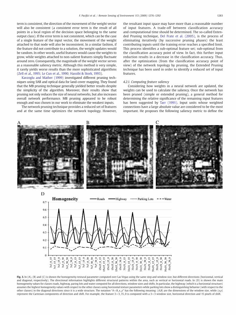
Fig. 3. In (A), (B) and (C) is shown the homogeneity textural parameter computed over Las Vand diagonal, respectively). The directional information highlights different structural pathomogeneity values for classes roads, highway, paring lots and water computed for all directiassumes the highest homogeneity values with respect to the other classes using horizontal teother classes) in the diagonal directions since it is a wide structure. The notation “A×B_x_yrepresent the Cartesian components of direction and shift. For example, the feature 3×3_1

the resultant input space may have more than a reasonable numberof input features. A trade-off between classification accuracyand computational time should be determined. The so-called Exten-ded Pruning technique, Del Frate et al. (2005), is the process ofeliminating iteratively (by successive pruning phases) the leastcontributing inputs until the training error reaches a specified limit.This process identifies a sub-optimal feature set; sub-optimal fromthe classification accuracy point of view. In fact, this further inputreduction results in a decrease in the classification accuracy. Thus,after the optimization (from the classification accuracy point ofview) of the network topology by pruning, the Extended Pruningtechnique has been used in order to identify a reduced set of inputfeatures.

4.2.1. Computing feature saliencyConsidering how weights in a neural network are updated, the

weights can be used to calculate the saliency. Once the network hasbeen pruned (simple or extended pruning), a general method fordetermining the relative significance of the remaining input featureshas been suggested by Tarr (1991). Input units whose weightedconnections have a large absolute value are considered to be the mostimportant. He proposes the following saliency metric to define the

egas using the same step and window size, but different directions (horizontal, verticalterns within the area, such as vertical or horizontal roads. In (D) is shown the mainons, window sizes and shifts. In particular, the highway (which is a horizontal structure)xture parameters while parking lots show a distinguishing behavior (with respect to the” has the following meaning: (A,B) are the dimensions of the window size, while (x,y)5_0 is computed with a 3×3 window size, horizontal direction and 15 pixels of shift.

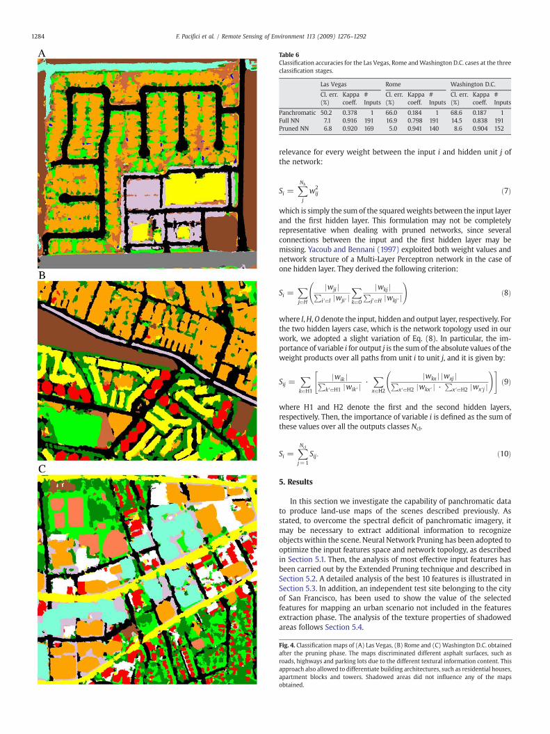
Table 6Classification accuracies for the Las Vegas, Rome andWashington D.C. cases at the threeclassification stages.

Las Vegas Rome Washington D.C.

Cl. err.(%)

Kappacoeff.

#Inputs

Cl. err.(%)

Kappacoeff.

#Inputs

Cl. err.(%)

Kappacoeff.

#Inputs

Panchromatic 50.2 0.378 1 66.0 0.184 1 68.6 0.187 1Full NN 7.1 0.916 191 16.9 0.798 191 14.5 0.838 191Pruned NN 6.8 0.920 169 5.0 0.941 140 8.6 0.904 152


relevance for every weight between the input i and hidden unit j ofthe network:

Si =XNh

j

w2ij ð7Þ

which is simply the sumof the squaredweights between the input layerand the first hidden layer. This formulation may not be completelyrepresentative when dealing with pruned networks, since severalconnections between the input and the first hidden layer may bemissing. Yacoub and Bennani (1997) exploited both weight values andnetwork structure of a Multi-Layer Perceptron network in the case ofone hidden layer. They derived the following criterion:

Si =XjaH

jwji jPiVaI jwjiVj

XkaO

jwkj jPj0aH jwkjVj

!ð8Þ

where I,H,O denote the input, hidden and output layer, respectively. Forthe two hidden layers case, which is the network topology used in ourwork, we adopted a slight variation of Eq. (8). In particular, the im-portance of variable i for output j is the sumof the absolute values of theweight products over all paths from unit i to unit j, and it is given by:

Sij =XkaH1

jwik jPkVaH1 jwikVj

·XxaH2

jwkx j jwxj jPxVaH2 jwkxVj ·

PxVaH2 jwxVj j

!" #ð9Þ

where H1 and H2 denote the first and the second hidden layers,respectively. Then, the importance of variable i is defined as the sum ofthese values over all the outputs classes Ncl.

Si =XNcl

j=1

Sij: ð10Þ

5. Results

In this section we investigate the capability of panchromatic datato produce land-use maps of the scenes described previously. Asstated, to overcome the spectral deficit of panchromatic imagery, itmay be necessary to extract additional information to recognizeobjects within the scene. Neural Network Pruning has been adopted tooptimize the input features space and network topology, as describedin Section 5.1. Then, the analysis of most effective input features hasbeen carried out by the Extended Pruning technique and described inSection 5.2. A detailed analysis of the best 10 features is illustrated inSection 5.3. In addition, an independent test site belonging to the cityof San Francisco, has been used to show the value of the selectedfeatures for mapping an urban scenario not included in the featuresextraction phase. The analysis of the texture properties of shadowedareas follows Section 5.4.

Fig. 4. Classification maps of (A) Las Vegas, (B) Rome and (C)Washington D.C. obtainedafter the pruning phase. The maps discriminated different asphalt surfaces, such asroads, highways and parking lots due to the different textural information content. Thisapproach also allowed to differentiate building architectures, such as residential houses,apartment blocks and towers. Shadowed areas did not influence any of the mapsobtained.

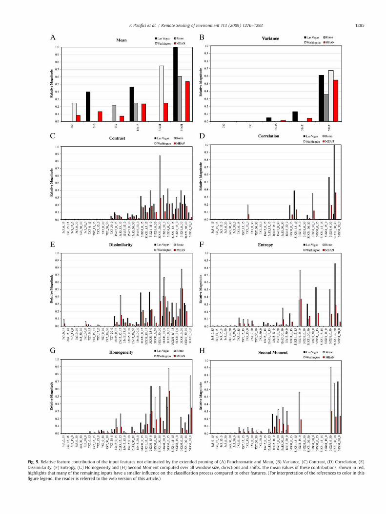
Fig. 5. Relative feature contribution of the input features not eliminated by the extended pruning of (A) Panchromatic and Mean, (B) Variance, (C) Contrast, (D) Correlation, (E)Dissimilarity, (F) Entropy, (G) Homogeneity and (H) Second Moment computed over all window size, directions and shifts. The mean values of these contributions, shown in red,highlights that many of the remaining inputs have a smaller influence on the classification process compared to other features. (For interpretation of the references to color in thisfigure legend, the reader is referred to the web version of this article.)


Fig. 6. Feature contributions with respect to textural parameters, window sizes anddirections. In (A) is shown the contributions of textural parameters regardless of thechoice of cell sizes and directions. Dissimilarity appears to be the most informativetexture parameter. In (B) is shown the importance of the cell sizes, regardless of thechoice of textural parameters and directions. In (C), the three directions (in black) andthe two-step size (in gray) show high and relatively similar contributions, meaning thatboth directions and step sizes are relevant for the classification phase.


5.1. Optimization of the feature space and network topology

The first effort has been to produce land-use maps using onlypanchromatic information with neural network. As expected, theresults obtained appeared to be really poor for the three test cases interms of classification accuracy. The obtained Kappa coefficient valuesare 0.378 for Las Vegas, 0.184 for Rome and 0.187 for Washington D.C.As expected, several of the defined classes were not recognized. Forexample, for the Las Vegas scene, only Bare Soil, Residential Houses,Roads and Short Vegetation have been identified, which are re-presentative of thematerials present in the area. This is shown in Fig. 2where it is possible to group the digital number values into four sets.Even though water and asphalt are different, it is well known from theliterature that they may assume similar values in panchromatic data.This has led to some confusion where water is grouped with roads,highway and parking lots.

As already explained in Section 3.1, a multi-scale textural inputspace has been extracted from panchromatic images (see Table 5),including first- and second-order textural parameters computed with5 window sizes, 3 directions and 2 step sizes. Note that directions andsteps are related only to second-order statistics. Fig. 3 shows anexample of the homogeneity parameter computed over Las Vegaswith three different directions (same step and window size). Asexpected, the direction calculation highlights different structural pat-terns within the area, such as vertical or horizontal roads, and parkinglots. In fact, the highway, which is a horizontal structure, has itshighest value in the 15_0 and 30_0 directions, while parking lots showa distinct behavior (with respect to the other classes) in the diagonaldirection since they arewide structures. Note, the notation “A×B_x_y”has the following meaning: (A,B) are the dimensions of the windowsize, while (x,y) represent the Cartesian components of direction andshift. For example, the feature 3×3_15_0 is computed with a 3×3window size, horizontal direction and 15 pixels of shift.

A considerable increase in classification accuracy has been obtainedusing the entire input dataset of 191 textural features. More precisely,Kappa coefficient values of 0.916 for Las Vegas, 0.798 for Romeand0.838for Washington D.C. have been obtained. With respect to the previousimplementation, all classeswere identified in the classificationmaps. Onthe other hand, as mentioned, a large input space rarely yields highclassification accuracies due to information redundancy. This results in anecessity to estimate the contribution of each parameter in order toreduce and optimize the input space. To this end, we adopted NeuralNetwork Pruning to eliminate the weakest connections, optimizing atthe same time the network topology. Generally, this process increasesthe classification accuracy by eliminating features that donot contributeto the classification process, but instead only introduce redundancy.After the pruning phase, the remaining inputs are 169 for Las Vegas,140for Rome and 152 forWashington D.C., respectively. This relatively smallfeature elimination resulted in a further increase of classificationaccuracy. In particular, the Kappa coefficient values increased to 0.920for Las Vegas, 0.941 for Rome and 0.904 for Washington D.C., whoseclassification maps are illustrated in Fig. 4 and the accuracies aresummarized in Table 6 for the reader's convenience. Taking into accountthe extension of boundary areas between objects, we noticed a slightdecrease of the classification accuracy for the Washington D. C. case,whose ground reference included boundary areas.

The obtained classification maps discriminated different asphaltsurfaces, such as roads, highways and parking lots due to the differenttextural information content. This approach also made it possible todifferentiate building architectures, sizes and heights, such asresidential houses, apartment blocks and towers. Here, it is importantto note that shadowed areas did not influence any of the mapsobtained. The reason for this will be described later in the paper. Theaccuracies obtainedwith the optimization of the network topology areconsidered here as an upper bound of the classification accuraciesderived from the multi-scale approach.

5.2. Features selection by extended pruning technique

In the previous section, the network pruning technique provided areduced set of textural features and an optimized network topology inorder to obtain the most accurate classification map. However, theinput space is not close to a reduced number of features relative to the


computational time, and a trade-off between classification accuracyand computational time should be found. The so-called ExtendedPruning technique is the process of eliminating the least contributinginputs, even from this optimal classification, in order to identify aminimal sub-optimal textural feature set. The resulting classificationis sub-optimal from the classification accuracy point of view, since thisfurther input reduction results in a decrease in the classificationaccuracy. Particularly, the criterion chosen to stop the extendedpruning phase was to reach a classification accuracy of about 0.800 interms of Kappa coefficient.

After the extended pruning phase, the remaining inputs are 59 forLas Vegas, 61 for Rome and 59 for Washington D.C., with accuracies(Kappa coeff.) decreased to 0.859, 0.820 and 0.796, respectively. InFig. 5 we present the relative contributions of the input features(including the panchromatic image itself), which are not eliminatedby the extended pruning. The saliency metric used to compute thefeature contributions has been illustrated in Sec. 4.1, Eqs. (9) and (10).Moreover, we normalized all the contribution values between 0 and 1,where 0 means no contribution to the classification phase. As shown,the contribution of each input varies from city to city, due to thearchitectural peculiarities (and diversity) of them. The analysis of themean values of these contributions, shown in red, clearly indicatesthat many of the remaining inputs have a smaller influence on theclassification process compared to other features. This means thatusing certain textural features (including different cell sizes anddirections) may have more significance than others.

To analyze the importance of textural parameters regardless ofthe choice of cell sizes and directions, we computed, for each ofthem, the feature contributions as sums over the different cell sizesand directions. As shown in Fig. 6A, the panchromatic band, whichdoes not contain any information on cell sizes and directions, hasthe smallest contribution. Fist-order textural features, which do notcontain any information on directions, have smaller contributionsthan second-order features. Particularly, Dissimilarity appears to bethe most informative texture parameter, even if it is similar toContrast. This may be related to the linear weighting of the gray-tone levels of the scene (to be compared to the exponentiallyweight of Contrast). In the same way, we analyzed the importanceof the cell sizes, regardless of the choice of textural parameters and

Fig. 7. Frequency of the input features with respect to the input feature contribution h

directions. This is illustrated in Fig. 6B, where larger cell sizes of31×31 and 51×51 show higher contributions. This may be relatedto the very high-resolution data used in this paper. Since QuickBirdandWorldView-1 sensors have resolutions close to half a meter, it isreasonable that the textural information is contained in the spatialrange of 15.0–25.0 m, a result which is consistent with Small(2003).

In Fig. 6C, the three directions (in black) and the two-step sizes (ingray) have high and similar contributions, meaning that both di-rections and step sizes are relevant for the classification phase. Thislast result points out the necessity of having directional information tobetter capture differences in textural patterns.

5.3. Analysis of the best 10 textural features

We have shown that many of the remaining inputs, after theextending pruning phase, have a smaller influence on the classifica-tion process compared to other features. To further investigate in-dividual feature contributions, the frequency of the input featureswith respect to the input feature contribution is shown in Fig. 7, whichhighlights that only very few inputs show a relative contributiongreater than 0.30. The best ten features are reported in Table 7 withthe corresponding values of contribution relative to the mean valuesover three cities and several different land-uses.

To understand the contribution of a single class to these tenfeatures, we merged together the different land-use classes into fivegroups, which are common to the three scenes. The resultant commonfive classes are: Buildings, Roads, Soil, Trees and Vegetation. Thecontributions per single class of the ten best features with respect tothese five classes are illustrated in Fig. 8. For example, the first-orderMean 51×51 seems to be appropriate for the discrimination of roads,while Dissimilarity 51×51_0_30 appears to be valuable for thedetection of trees.

With this drastic reduction of input features (from about 60 to 10),we expected a further decrease of the classification accuracy withrespect to the extended pruning results. On the other hand, this effectwas compensated for by the reduction (from about 11 to 5) of theoutput classes. In particular, we re-classified the Washington D.C.scene using only the ten best textural inputs, obtaining an accuracy of

ighlights that only very few inputs show a relative contribution greater than 0.30.

Table 7Best ten features and corresponding feature contribution averaged over three cities andseveral different land-uses classes.

Best 10 features Relative input feature contribution

Mean 51×51 0.535Variance 51×51 0.547Homogeneity 51×51_0_15 0.572Homogeneity 51×51_30_0 0.345Dissimilarity 31×31_30_30 0.339Dissimilarity 31×31_30_0 0.404Dissimilarity 51×51_0_30 0.512Entropy 31×31_15_0 0.374Second Moment 51×51_0_30 0.301Correlation 51×51_30_30 0.357


0.861. This result is particularly relevant since it was obtained after ageneralization (mean) of results obtained over all of the cities withdifferent architectures.

Even though these considerations show similarities, especially interms of computational time and generalization capability fordifferent urban scenarios, it is necessary to emphasize the importanceof exploiting the entire textural features dataset, including all differentspatial scales and directions. Starting from the same textural featuresand pruning the neural networks made it possible to classify differenturban scenarios with high accuracies, showing both the efficiency andthe robustness of the multi-scale approach used here.

5.3.1. The San Francisco test caseIn the previous section, we discussed the feature contributions as

mean values over three different test sets corresponding to Las Vegas,Rome and Washington D.C. A reduced set of ten features has beenidentified as valuable for urban classification. Now the question is:how well do these ten features classify a new urban scene? To answerthis question, we used these ten features to classify an independentdata set of a portion of San Francisco. Note that different combinationsof texture metrics might produce more accurate results for thisparticular test case. However, we only want to investigate thepotentialities of the selected features (obtained as average of 3 totallydifferent conditions) when applied to a new scenario. In this sense,these ten features are not an optimal combination, but simply a set ofinputs that may potentially increase the classification accuracy whenapplied to very high-resolution imagery.

Fig. 8. Contributions per single class of the best ten features with respect to the five commonfor the discrimination of roads than Correlation or Second Moment, while Dissimilarity 51×

The scene, shown in Fig. 9A, has been imaged by WorldView-1with an off-nadir angle of 19.6°. Further, long shadows are caused by asun elevation of 29.6°. This neighborhood may be considered arepresentative architecture for many cities, making it suitable forvalidation purposes. The same five common classes defined previouslyhave been used. Training and validation pixels have been selected andare summarized in Table 8, while the entire ground reference map isshown in Fig. 9B.

We first classified the panchromatic image alone, obtaining aKappa coefficient of about 0.224. Then, using only the reduced set often textural features, we obtained a map, shown in Fig. 9C, whoseaccuracy was about 0.917.

5.4. Analysis of texture properties of shadowed areas

Shadow effects are often ignored when using decametric spatialresolution images, such as Landsat. In these cases, shadowed pixelsmay be located on an object's boundaries where there is a mixture ofradiances caused by different surfaces. Vice versa, shadows have ahuge impact on classification with metric or sub-metric spatialresolution images, such as QuickBird or WorldView-1. In urbanareas, shadows are mainly caused by buildings, tress or bridges andmay potentially provide additional geometric and semantic informa-tion on the shape and orientation of objects. On the other hand,shadowed surfaces require more consideration since they may cause aloss of information or a shape distortion of objects.

In the literature, shadow is generally dealt with as an additionalclass (Benediktsson et al., 2005; Bruzzone and Carlin, 2006). In thispaper, we have defined the ground reference regardless of thepresence of shadowed areas, leading to classification maps, whichdo not contain any pixels of shadow. To further investigate this, weextracted the shadowed pixels of the Rome scene and analyzed theirtextural values (normalized between 0 and 1) with respect to the non-shadowed pixels of the same class. As illustrated in Fig. 10, wherecontinuous-lines represent pixels of shadowand dotted-lines the non-shadowed pixels of the corresponding class. Only panchromaticinformation appears to not be able to adequately separate the classeswhose pixels are covered by shadow. In fact, they are mainlyconcentrated in the lower part of the scale values, acting more as aunique class. Mean values (and their standard deviation) are alsoreported in Table 9 for blocks, roads and vegetation. Even though these

classes defined. The first-order Mean and Variance 51×51 seem to be more appropriate51_0_30 appears to be valuable for the detection of trees.

Table 8San Francisco case: classes, training and validation samples, and color legend.


surfaces are different, the (normalized) panchromatic values ofshadowed areas are very similar: 0.08, 0.05 and 0.07, respectively.By contrast, shadowed areas have their own texture properties,allowing the discrimination between different shadowed classes.

To make Fig. 10 clearer, we only consider the class buildings(including both apartment blocks and towers), which is one of themost relevant for urban classification. Shadows of buildings aremainly due to two different effects: i) shadows of the building on itselfand ii) shadows of other objects, such as other buildings or trees, on abuilding. As shown in Fig. 11, buildings show a sort of characteristictextural signature. For example, the variance of shadowed buildings isslightly higher than non-shadowed buildings. This may be interpretedby considering the smaller extension in the area of shadow withrespect to buildings (for the scene considered) and the higher contrastin terms of gray-tone levels on the boundary between shadowed andnon-shadowed pixels. Smaller objects with higher contrast lead tohigher spatial variability, thus larger variance values. Similar con-siderations may be given to the homogeneity feature, which showsan inversion of the trend between shadowed and non-shadowedbuildings due to the larger step size (30 instead of 15 pixels), but equalwindow size of 51×51 pixels.

6. Conclusion

In this work, we investigated the potential of very high-resolution panchromatic QuickBird and WorldView-1 imagery toclassify the land-use of urban environments. Spectral-based classi-fication methods may fail with the increased geometrical resolutionof the data available. In fact, improved spatial resolution dataincreases within-class variances, which results in high interclassspectral confusion. In many cases, several pixels are representative ofobjects, which are not part of land-use classes defined. This problemis intrinsically related to the sensor resolution and it cannot besolved by increasing the number of spectral channels. To overcomethe spectral information deficit of panchromatic imagery, it isnecessary to extract additional information to recognize objectswithin the scene.

The multi-scale approach discussed in this paper exploits thecontextual information of first- and second-order textural features tocharacterize the land-use. For this purpose, textural parameters havebeen systematically investigated computing the features over fivedifferent window sizes, three different directions and two differentcell shifts for a total of 191 inputs. Neural Network Pruning andsaliency measurements allowed the optimization of the networktopology and give an indication of the most important texturalfeatures for sub-metric spatial resolution imagery and urbanscenarios.

Fig. 9. (A) Panchromatic image and (B) ground reference of San Francisco. In (C) isshown the classification map obtained using the reduced set of ten textural features.Color codes are in Table 8. (For interpretation of the references to color in this figurelegend, the reader is referred to the web version of this article.)

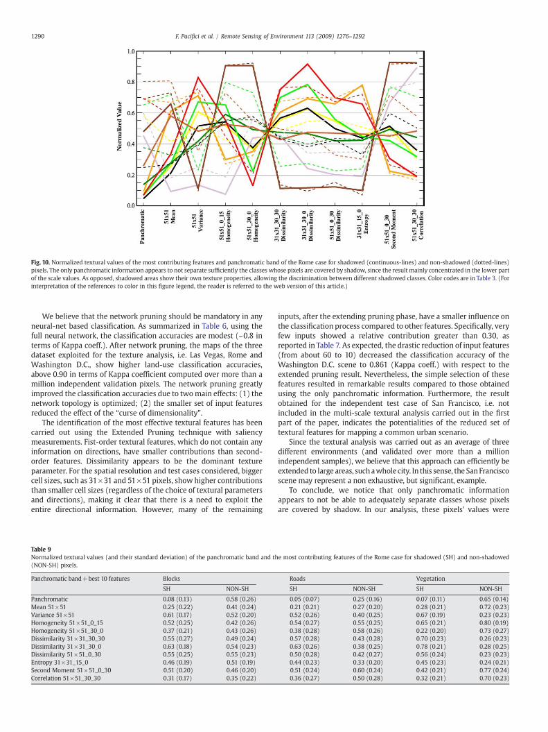
Fig. 10. Normalized textural values of the most contributing features and panchromatic band of the Rome case for shadowed (continuous-lines) and non-shadowed (dotted-lines)pixels. The only panchromatic information appears to not separate sufficiently the classes whose pixels are covered by shadow, since the result mainly concentrated in the lower partof the scale values. As opposed, shadowed areas show their own texture properties, allowing the discrimination between different shadowed classes. Color codes are in Table 3. (Forinterpretation of the references to color in this figure legend, the reader is referred to the web version of this article.)


We believe that the network pruning should be mandatory in anyneural-net based classification. As summarized in Table 6, using thefull neural network, the classification accuracies are modest (~0.8 interms of Kappa coeff.). After network pruning, the maps of the threedataset exploited for the texture analysis, i.e. Las Vegas, Rome andWashington D.C., show higher land-use classification accuracies,above 0.90 in terms of Kappa coefficient computed over more than amillion independent validation pixels. The network pruning greatlyimproved the classification accuracies due to twomain effects: (1) thenetwork topology is optimized; (2) the smaller set of input featuresreduced the effect of the “curse of dimensionality”.

The identification of the most effective textural features has beencarried out using the Extended Pruning technique with saliencymeasurements. Fist-order textural features, which do not contain anyinformation on directions, have smaller contributions than second-order features. Dissimilarity appears to be the dominant textureparameter. For the spatial resolution and test cases considered, biggercell sizes, such as 31×31 and 51×51 pixels, show higher contributionsthan smaller cell sizes (regardless of the choice of textural parametersand directions), making it clear that there is a need to exploit theentire directional information. However, many of the remaining

Table 9Normalized textural values (and their standard deviation) of the panchromatic band and th(NON-SH) pixels.

Panchromatic band+best 10 features Blocks

SH NON-SH

Panchromatic 0.08 (0.13) 0.58 (0.26)Mean 51×51 0.25 (0.22) 0.41 (0.24)Variance 51×51 0.61 (0.17) 0.52 (0.20)Homogeneity 51×51_0_15 0.52 (0.25) 0.42 (0.26)Homogeneity 51×51_30_0 0.37 (0.21) 0.43 (0.26)Dissimilarity 31×31_30_30 0.55 (0.27) 0.49 (0.24)Dissimilarity 31×31_30_0 0.63 (0.18) 0.54 (0.23)Dissimilarity 51×51_0_30 0.55 (0.25) 0.55 (0.23)Entropy 31×31_15_0 0.46 (0.19) 0.51 (0.19)Second Moment 51×51_0_30 0.51 (0.20) 0.46 (0.20)Correlation 51×51_30_30 0.31 (0.17) 0.35 (0.22)

inputs, after the extending pruning phase, have a smaller influence onthe classification process compared to other features. Specifically, veryfew inputs showed a relative contribution greater than 0.30, asreported in Table 7. As expected, the drastic reduction of input features(from about 60 to 10) decreased the classification accuracy of theWashington D.C. scene to 0.861 (Kappa coeff.) with respect to theextended pruning result. Nevertheless, the simple selection of thesefeatures resulted in remarkable results compared to those obtainedusing the only panchromatic information. Furthermore, the resultobtained for the independent test case of San Francisco, i.e. notincluded in the multi-scale textural analysis carried out in the firstpart of the paper, indicates the potentialities of the reduced set oftextural features for mapping a common urban scenario.

Since the textural analysis was carried out as an average of threedifferent environments (and validated over more than a millionindependent samples), we believe that this approach can efficiently beextended to large areas, suchawhole city. In this sense, the SanFranciscoscene may represent a non exhaustive, but significant, example.

To conclude, we notice that only panchromatic informationappears to not be able to adequately separate classes whose pixelsare covered by shadow. In our analysis, these pixels' values were

e most contributing features of the Rome case for shadowed (SH) and non-shadowed

Roads Vegetation

SH NON-SH SH NON-SH

0.05 (0.07) 0.25 (0.16) 0.07 (0.11) 0.65 (0.14)0.21 (0.21) 0.27 (0.20) 0.28 (0.21) 0.72 (0.23)0.52 (0.26) 0.40 (0.25) 0.67 (0.19) 0.23 (0.23)0.54 (0.27) 0.55 (0.25) 0.65 (0.21) 0.80 (0.19)0.38 (0.28) 0.58 (0.26) 0.22 (0.20) 0.73 (0.27)0.57 (0.28) 0.43 (0.28) 0.70 (0.23) 0.26 (0.23)0.63 (0.26) 0.38 (0.25) 0.78 (0.21) 0.28 (0.25)0.50 (0.28) 0.42 (0.27) 0.56 (0.24) 0.23 (0.23)0.44 (0.23) 0.33 (0.20) 0.45 (0.23) 0.24 (0.21)0.51 (0.24) 0.60 (0.24) 0.42 (0.21) 0.77 (0.24)0.36 (0.27) 0.50 (0.28) 0.32 (0.21) 0.70 (0.23)

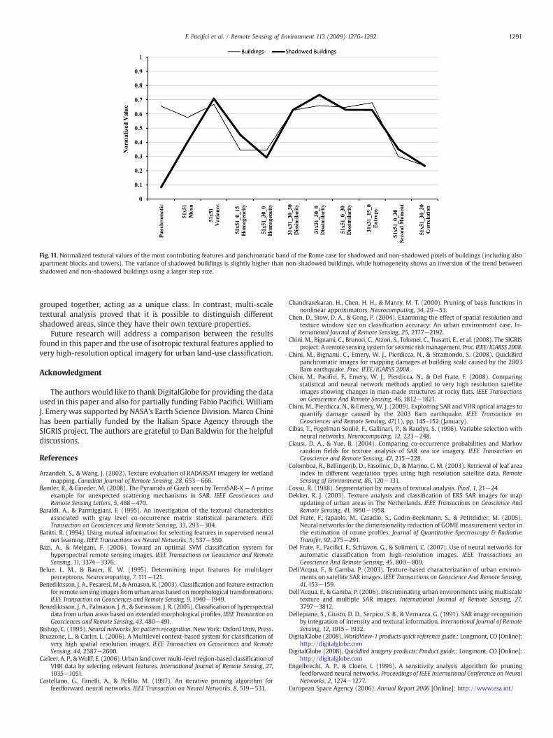
Fig. 11. Normalized textural values of the most contributing features and panchromatic band of the Rome case for shadowed and non-shadowed pixels of buildings (including alsoapartment blocks and towers). The variance of shadowed buildings is slightly higher than non-shadowed buildings, while homogeneity shows an inversion of the trend betweenshadowed and non-shadowed buildings using a larger step size.


grouped together, acting as a unique class. In contrast, multi-scaletextural analysis proved that it is possible to distinguish differentshadowed areas, since they have their own texture properties.

Future research will address a comparison between the resultsfound in this paper and the use of isotropic textural features applied tovery high-resolution optical imagery for urban land-use classification.

Acknowledgment

The authors would like to thank DigitalGlobe for providing the dataused in this paper and also for partially funding Fabio Pacifici. WilliamJ. Emery was supported by NASA's Earth Science Division. Marco Chinihas been partially funded by the Italian Space Agency through theSIGRIS project. The authors are grateful to Dan Baldwin for the helpfuldiscussions.

References

Arzandeh, S., & Wang, J. (2002). Texture evaluation of RADARSAT imagery for wetlandmapping. Canadian Journal of Remote Sensing, 28, 653−666.

Bamler, R., & Eineder, M. (2008). The Pyramids of Gizeh seen by TerraSAR-X — A primeexample for unexpected scattering mechanisms in SAR. IEEE Geosciences andRemote Sensing Letters, 5, 468−470.

Baraldi, A., & Parmiggiani, F. (1995). An investigation of the textural characteristicsassociated with gray level co-occurrence matrix statistical parameters. IEEETransaction on Geosciences and Remote Sensing, 33, 293−304.

Batitti, R. (1994). Using mutual information for selecting features in supervised neuralnet learning. IEEE Transactions on Neural Networks, 5, 537−550.

Bazi, A., & Melgani, F. (2006). Toward an optimal SVM classification system forhyperspectral remote sensing images. IEEE Transactions on Geoscience and RemoteSensing, 11, 3374−3376.

Belue, L. M., & Bauer, K. W. (1995). Determining input features for multilayerperceptrons. Neurocomputing, 7, 111−121.

Benediktsson, J. A., Pesaresi, M., & Arnason, K. (2003). Classification and feature extractionfor remote sensing images fromurban areas based onmorphological transformations.IEEE Transaction on Geosciences and Remote Sensing, 9, 1940−1949.

Benediktsson, J. A., Palmason, J. A., & Sveinsson, J. R. (2005). Classification of hyperspectraldata from urban areas based on extended morphological profiles. IEEE Transaction onGeosciences and Remote Sensing, 43, 480−491.

Bishop, C. (1995). Neural networks for pattern recognition. New York: Oxford Univ, Press.Bruzzone, L., & Carlin, L. (2006). A Multilevel context-based system for classification of

very high spatial resolution images. IEEE Transaction on Geosciences and RemoteSensing, 44, 2587−2600.

Carleer, A. P., &Wolff, E. (2006). Urban land covermulti-level region-based classification ofVHR data by selecting relevant features. International Journal of Remote Sensing, 27,1035−1051.

Castellano, G., Fanelli, A., & Pelillo, M. (1997). An iterative pruning algorithm forfeedforward neural networks. IEEE Transaction on Neural Networks, 8, 519−531.

Chandrasekaran, H., Chen, H. H., & Manry, M. T. (2000). Pruning of basis functions innonlinear approximators. Neurocomputing, 34, 29−53.

Chen, D., Stow, D. A., & Gong, P. (2004). Examining the effect of spatial resolution andtexture window size on classification accuracy: An urban environment case. In-ternational Journal of Remote Sensing, 25, 2177−2192.

Chini, M., Bignami, C., Brunori, C., Atzori, S., Tolomei, C., Trasatti, E., et al. (2008). The SIGRISproject: A remote sensing system for seismic riskmanagement. Proc. IEEE/IGARSS 2008.

Chini, M., Bignami, C., Emery, W. J., Pierdicca, N., & Stramondo, S. (2008). QuickBirdpanchromatic images for mapping damages at building scale caused by the 2003Bam earthquake. Proc. IEEE/IGARSS 2008.

Chini, M., Pacifici, F., Emery, W. J., Pierdicca, N., & Del Frate, F. (2008). Comparingstatistical and neural network methods applied to very high resolution satelliteimages showing changes in man-made structures at rocky flats. IEEE Transactionson Geoscience And Remote Sensing, 46, 1812−1821.

Chini, M., Pierdicca, N., & Emery, W. J. (2009). Exploiting SAR and VHR optical images toquantify damage caused by the 2003 Bam earthquake. IEEE Transaction onGeosciences and Remote Sensing, 47(1), pp. 145–152 (January).

Cibas, T., Fogelman Soulié, F., Gallinari, P., & Raudys, S. (1996). Variable selection withneural networks. Neurocomputing, 12, 223−248.

Clausi, D. A., & Yue, B. (2004). Comparing co-occurrence probabilities and Markovrandom fields for texture analysis of SAR sea ice imagery. IEEE Transaction onGeoscience and Remote Sensing, 42, 215−228.

Colomboa, R., Bellingerib, D., Fasolinic, D., & Marino, C. M. (2003). Retrieval of leaf areaindex in different vegetation types using high resolution satellite data. RemoteSensing of Environment, 86, 120−131.

Cossu, R. (1988). Segmentation by means of textural analysis. Pixel, 1, 21−24.Dekker, R. J. (2003). Texture analysis and classification of ERS SAR images for map

updating of urban areas in The Netherlands. IEEE Transactions on Geoscience AndRemote Sensing, 41, 1950−1958.

Del Frate, F., Iapaolo, M., Casadio, S., Godin-Beekmann, S., & Petitdidier, M. (2005).Neural networks for the dimensionality reduction of GOME measurement vector inthe estimation of ozone profiles. Journal of Quantitative Spectroscopy & RadiativeTransfer, 92, 275−291.

Del Frate, F., Pacifici, F., Schiavon, G., & Solimini, C. (2007). Use of neural networks forautomatic classification from high-resolution images. IEEE Transactions onGeoscience And Remote Sensing, 45, 800−809.

Dell'Acqua, F., & Gamba, P. (2003). Texture-based characterization of urban environ-ments on satellite SAR images. IEEE Transactions on Geoscience And Remote Sensing,41, 153−159.

Dell'Acqua, F., & Gamba, P. (2006). Discriminating urban environments using multiscaletexture and multiple SAR images. International Journal of Remote Sensing, 27,3797−3812.

Dellepiane, S., Giusto, D. D., Serpico, S. B., & Vernazza, G. (1991). SAR image recognitionby integration of intensity and textural information. International Journal of RemoteSensing, 12, 1915−1932.

DigitalGlobe (2008).WorldView-1 products quick reference guide.: Longmont, CO [Online]:http://digitalglobe.com

DigitalGlobe (2008). QuickBird imagery products: Product guide.: Longmont, CO [Online]:http://digitalglobe.com

Engelbrecht, A. P., & Cloete, I. (1996). A sensitivity analysis algorithm for pruningfeedforward neural networks. Proceedings of IEEE International Conference on NeuralNetworks, 2, 1274−1277.

European Space Agency (2006). Annual Report 2006 [Online]: http://www.esa.int/

http://digitalglobe.com

http://digitalglobe.com

http://www.esa.int/


Foody, G. M. (2002). Status of land cover classification accuracy assessment. RemoteSensing of Environment, 80, 185−201.

Foroutan, I., & Sklansky, J. (1987). Feature selection for automatic classification of non-Gaussian data. IEEE Transactions on Systems, Man, and Cybernetics, 17, 187−198.

GLP (2005). Science plan and implementation strategy. IGBP Report No. 53/IHDP ReportNo. 19. Stockholm: IGBP Secretariat.

Gong, P., Marceau, D. J., & Howarth, P. J. (1992). A comparison of spatial featureextraction algorithms for land-use classification with SPOT HRV data. RemoteSensing of Environment, 40, 137−151.

Guyon, I., Weston, J., Barnhill, S., & Vapnik, V. (2002). Gene selection for cancerclassification using support vector machines. Machine Learning, 46, 389−422.

Haralick, R. M. (1979). Statistical and structural approaches to texture. Proceeding of theIEEE, 67, 786−804.

Haralick, R. M., Shanmuga, K., & Dinstein, I. H. (1973). Textural features for imageclassification. IEEE Transactions on Systems, Man, and Cybernetics, SMC, 3, 610−621.

Hassibi, B., & Stork, D. G. (1993). Second-order derivatives for network pruning:Optimal brain surgeon. In S. J. Hanson, J. D. Cowan, & C. L. Giles (Eds.), Advances inneural information processing systems 5 (pp. 164−171). San Mateo: MorganKaufmann.

Hirose, Y., Yamashita, K., & Hijiya, S. (1991). Back-propagation algorithm which variesthe number of hidden units. Neural Networks, 4, 61−66.

Holz, H. J., & Loew, M. H. (1994). Relative feature importance: A classifier independentapproach to feature selection. In E. S. Gelsema & L. N. Kanal (Eds.), Proceedings ofpattern recognition in practice IV: Multiple paradigms, comparative studies and hybridsystems (pp. 473–1823).

Karathanassi, V., Iossifidis, C., & Rokos, D. (2000). A texture-based classification methodfor classifying built areas according to their density. International Journal of RemoteSensing, 21, 1807−1823.

Karthaus, V., Thygesen, H., Egmont-Petersen, M., Talmon, J., Brender, J., & McNair, P.(1995). User-requirements driven learning. Computer Methods and Programs inBiomedicine, 48, 39−44.

Kavzoglu, T., & Mather, P. M. (1999). Pruning artificial neural networks: An exampleusing land cover classification of multi-sensor images. International Journal ofRemote Sensing, 20, 2787−2803.

Kittler, J. (1980). Computational problems of feature selection pertaining to large datasets. In E. S. Gelsema & L. N. Kanal (Eds.), Pattern recognition in practice (pp.405−414). : North Holland.

Kudo, M., & Shimbo, M. (1993). Feature selection based on the structural indices ofcategories. Pattern Recognition, 26, 891−901.

Kurosu, T., Uratsuka, S., Maeno, H., & Kozu, T. (1999). Texture statistics for classificationof land use with multitemporal JERS-1 SAR single-look imagery. IEEE Transaction onGeoscience and Remote Sensing, 37, 227−235.

Kurvonen, L., & Hallikainen, M. (1999). Textural information of multitemporal ERS-1and JERS-1 SAR images with application to land and forest type classification inboreal zone”. IEEE Transaction on Geoscience and Remote Sensing, 37, 680−689.

Landgrebe, D. A. (2003). Signal theory methods in multispectral remote sensing. Hoboken,New Jersey: John Wiley and Sons.

Le Cun, Y., Denker, J. S., & Solla, S. A. (1990). Optimal brain damage.. In D. S. Touretsky(Ed.), Advances in neural information processing systems 2 (pp. 598−605). SanMateo: Morgan Kaufmann.

Leray, P., & Gallinari, P. (1998). Feature selection with neural networks. BehaviormetricaUniversité Paris (pp. 6).

Mao, J., Mohiuddin, K., & Jain, A. K. (1994). Parsimonious network design and featureselection through node pruning. IEEE Proceedings of the 12th IAPR International.Conference on Pattern Recognition, Vol. 2. (pp. 622−624).

Onnia, V., Tico, M., & Saarinen, J. (2001). Feature selection method using neuralnetwork. IEEE Proceedings of the International Conference on Image Processing, Vol 1.(pp. 513−516).

Ouma, Y. O., Ngigi, T. G., & Tateishi, R. (2006). On the optimization and selection ofwavelet texture for feature extraction from high-resolution satellite imagery withapplication towards urban-tree delineation. International Journal of Remote Sensing,27, 73−104.

Pacifici, F., Del Frate, F., Solimini, C., & Emery, W. J. (2007). An innovative neural-netmethod to detect temporal changes in high-resolution optical satellite imagery.IEEE Transaction on Geoscience and Remote Sensing, 45, 2940−2952.

Pagot, E., & Martino Pesaresi, M. (2008). Systematic study of the urban postconflictchange classification performance using spectral and structural features in a

support vector machine. IEEE Journal Of Selected Topics In Applied Earth ObservationsAnd Remote Sensing, 2, 120−128.

Pesaresi, M. (2000). Texture analysis for urban pattern recognition using fine-resolutionpanchromatic satellite imagery. Geographical & Environmental Modelling, 4, 43−63.

Puissant, A., Hirsch, J., & Weber, C. (2005). The utility of texture analysis to improve per-pixel classification for high to very high spatial resolution imagery. InternationalJournal of Remote Sensing, 26, 733−745.

Reed, R. (1993). Pruning algorithms— A survey. IEEE Transactions on Neural Networks, 4,740−747.

Shaban, M. A., & Dikshit, O. (2001). Improvement of classification in urban areas by theuse of textural features: The case study of Lucknow city, Uttar Pradesh. InternationalJournal of Remote Sensing, 22, 565−593.

Shaban, M. A., & Dikshit, O. (2002). Evaluation of the merging of SPOTmultispectral andpanchromatic data for classification of an urban environment. International Journalof Remote Sensing, 23, 249−262.

Shackelford, A. K., & Davis, C. H. (2003). A Hierarchical fuzzy classification approach forhigh-resolutionmultispectral data over urban areas. IEEE Transactions on Geoscienceand Remote Sensing, 9, 1920−1932.

Shanmugan, K. S., Narayanan, V., Frost, V. S., Stiles, J. A., & Holtzman, J. C. (1981). Texturalfeatures for Dadar image analysis. IEEE Transactions on Geoscience and RemoteSensing, 19, 153−156.

Sietsma, J., & Dow, R. J. F. (1998). Neural net pruning: Why and how. IEEE Proceedings ofthe International Conference on Neural Networks, Vol 1. (pp. 325−333).

Small, C. (2003). High spatial resolution spectral mixture analysis of urban reflectance.Remote Sensing of Environment, 88, 170−186.

Stahlberger, A., & Riedmiller, M. (1997). Fast network pruning and feature extractionusing the unit-OBS algorithm. In M. C. Mozer, M. I. Jordan, & T. Petsche (Eds.),Advances in neural information processing systems (pp. 655−660). MA: MorganKaufmann.

Suzuki, K., Horiba, I., & Sugie, N. (2001). A simple neural network pruning algorithmwith application to filter synthesis. Neural Processing Letters, 13, 43−53.

Tarr, G., (1991).Multi-layered feedforward neural networks for image segmentation, Ph. D.dissertation, School of Engineering, Air Force Institute of Technology. Wright-Patterson AFB OH.

Tatem, A. J. T., Noorb, A. M., & Hay, S. I. (2005). Assessing the accuracy of satellite derivedglobal and national urban maps in Kenya. Remote Sensing of Environment, 96,87−97.

Treitz, P. M., Howarth, P. J., Filho, P. J., & Soulis, E. D. (2000). Agricultural cropclassification using SAR tone and texture statistics. Canadian Journal of RemoteSensing, 26, 18−29.

Tuceryan, M., & Jain, A. K. (1993). Texture analysis. In C. Chen, L. Pau, & P. Wang (Eds.),Handbook of pattern recognition and computer vision Singapore: World Scientific.

Verikas, A., & Bacauskiene, M. (2002). Feature selection with neural networks. PatternRecognition Letters, 23, 1323−1335.

Voigt, S., Kemper, T., Riedlinger, T., Kiefl, R., Scholte, K., &Mehl, H. (2007). Satellite imageanalysis for disaster and crisis-management support. IEEE Transactions onGeoscience and Remote Sensing, 6, 1520−1528.

Weston, J., Elisseeff, A., Schölkopf, B., & Tipping,M. (2003).Useof the zero-normwith linearmodels and kernel methods. Journal of Machine Learning Research, 3, 1439−1461.

Yacoub, M., & Bennani, Y. (1997). HVS: A heuristic for variable selection in multilayerartificial neural network classifier. In C. Dagli, M. Akay, O. Ersoy, B. Fernandez, &A. Smith (Eds.), Intelligent engineering systems through artificial neural networks(pp. 527−532). Missouri, USA: St Louis.

Zell, A., et al. (1995). SNNS, Stuttgart Neural Network Simulator, user manual. Universityof Stuttgart Germany: Stuttgart www.ra.informatik.uni-tuebingen.de/SNNS

Zeng, X., & Yeung, D. S. (2006). Hidden neuron pruning of multilayer perceptrons usinga quantified sensitivity measure. Neurocomputing, 69, 825−837.

Zhang, Q., & Couloigner, I. (2006). Benefit of the angular texture signature for theseparation of parking lots and roads on high resolution multi-spectral imagery.Pattern Recognition Letters, 27, 937−946.

Zhang, Q., Wang, J., Gong, P., & Shi, P. (2003). Study of urban spatial patterns from SPOTpanchromatic imagery using textural analysis. International Journal of RemoteSensing, 24, 4137−4160.

http://www.ra.informatik.uni-tuebingen.de/SNNS

a neural network approach using multi-scale textural metrics from very high-resolution panchromatic...

Documents