1

A network-based approach for estimating pedestrian journey-time exposure to air pollution

Gemma Davies* and J. Duncan Whyatt

Lancaster Environment Centre, Lancaster University, Lancaster, Lancashire, LA1 4YQ, UK * Corresponding author: Tel: +44 (0)1524 510252. Email addresses: gemma.davies@lancaster.ac.uk. (G. Davies), d.whyatt@lancaster.ac.uk (J.D. Whyatt).

Abstract

Individual exposure to air pollution depends not only upon pollution concentrations in the surrounding environment, but also on the volume of air inhaled, which is determined by an individual’s physiology and activity level. This study focuses on journey-time exposure, using network analysis in a GIS environment to identify pedestrian routes between multiple origins and destinations throughout the city of Lancaster, North West England. For each segment of a detailed footpath network, exposure was calculated accounting for PM2.5 concentrations (estimated using an atmospheric dispersion model) and respiratory minute volume (varying between individuals and with slope). For each of the routes generated the cumulative exposure to PM2.5 was estimated, allowing for easy comparison between multiple routes.

Significant variations in exposure were found between routes depending on their geography, as well as in response to variations in background concentrations and meteorology between days. Differences in physiological characteristics such as age or weight were also seen to impact journey-time exposure considerably. In addition to assessing exposure for a given route, the approach was used to identify alternative routes that minimised journey-time exposure. Exposure reduction potential varied considerably between days, with even subtle shifts in route location, such as to the opposite side of the road, showing significant benefits.

The method presented is both flexible and scalable, allowing for the interactions between physiology, activity level, pollution concentration and journey duration to be explored. In enabling physiology and activity level to be integrated into exposure calculations a more comprehensive estimate of journey-time exposure can be made, which has potential to provide more realistic inputs for epidemiological studies.

Key words: PM2.5; journey-time exposure; air pollution modelling; GIS network analysis; physiology.

1. Introduction

Evidence indicates that transport-related air pollution has a number of health implications including mortality (Heinrich et al, 2005). These include short-term effects such as irritation to eyes, nose and throat, upper respiratory infections, headaches, nausea and allergic illness such as asthma. Long term effects include chronic respiratory disease, cancer, heart disease and even brain damage. Ambient air pollution has also been linked with low birth weight (Xia and Tong, 2006; Heinrich et al, 2005; Krzyzanowski, 2005; RCEP, 2007; Pedersen et al, 2013). Health impacts from transport-related air pollution may occur in response to a single journey (McCreanor et al, 2007; Peters et al 2004) Reducing exposure to transport-related air pollution is therefore a key target for public health (RCEP, 2007; Künzli et al, 2000).

An individual’s exposure to air pollution depends on the duration of exposure and volume of pollutants inhaled (Xia and Tong, 2006). Inhalation rates depend on both an individual’s physiology and activity level. The main atmospheric pollutants affecting public health include nitrogen dioxide (NO2), particulates, sulphur dioxide (SO2) and ozone (O3) (Xia and Tong, 2006). Of these, particulates have the longest cumulative effect

2

on health as they contain materials not easily digested and resolved by the body, and can be deposited in the nose, throat and lungs (Xia and Tong, 2006). This study will therefore concentrate on particulate matter less than 2.5 µm in diameter (PM2.5) as other researchers have shown that these are of greatest concern for human health (Pope and Dockery, 2006; Schwartz and Neas, 2000). PM2.5 a is non-threshold pollutant, with health impacts potentially occurring even with low concentrations (RCEP, 2007; Pope and Dockery, 2006).

While the proportion of an individual’s time spent in transit is relatively small it can account for a disproportionately high amount of their exposure to air pollution. The impact of journey-time exposure on health is therefore potentially significant (Gulliver and Briggs, 2005). For example, when evaluating personal exposure to Black Carbon, Dons et al (2012) found that while only 6.3% of participants time was spent in transport, this corresponded to 21% of their personal exposure. Some studies have sought to calculate journey-time exposure using monitoring (Yu et al 2012, Gómez-Perales et al 2004; Chan et al 2002); however this approach is necessarily limited in the number of potential routes for which exposure estimates can be determined. Attempts have been sought to address this challenge modelling both pollutant concentrations and potential route choices (Gulliver and Briggs, 2005; Hertel et al, 2008). However, very little research into journey-time exposure accounts for physiology and activity level despite their significance in influencing individual exposure (inhaled dose). One exception to this is the work by Int Panis et al (2010) who recognise the importance of considering inhaled dose when comparing exposure between cyclists and car passengers, using monitoring techniques to record particulate concentrations and respiratory measurements. However, consideration of respiratory rates remains conspicuously absent from most other studies.

The aim of this paper is to present a method for calculating journey-time exposure between any combination of origins and destinations, incorporating not only duration of journey and pollution concentrations as considered by Gulliver and Briggs (2005), but accounting also for physiology and activity level, thus enabling exposure to be calculated as inhaled dose (µg) rather than ambient exposure (µg.m-3). This study will focus entirely on pedestrians and hence consider only outdoor exposure, however, the same approach could be applied to other transport modes, or multimodal networks. In considering pedestrians only, the range of activity levels to be considered is reduced and the need to scale pollutant concentrations for different transport modes is avoided. Typically ‘in vehicle’ modes of transport are associated with lower activity levels than walking or cycling and therefore lower respiratory rates and potentially lower inhaled exposure. This, however, needs to be balanced against the potential health benefits of increased activity levels (de Hartog et al, 2010). As exposure generally peaks during peak commuting hours (Briggs, 2005; Dons et al, 2013) the case study presented focuses on 08:00 to 09:00 in the morning, with traffic flow data representing typical rush hour conditions. The method will also be applied to explore the potential to reduce journey-time exposure by determining routes of least exposure in addition to fastest routes. The network developed for the purpose of this analysis includes footpaths on either side of main roads, thus enabling the contrast in exposure between different sides of the road to be considered (Greaves et al, 2008).

3

Figure 1: Modelled factors affecting journey-time exposure to air pollution

This paper demonstrates the application of network analysis within a Geographic Information System (GIS) to calculate walking routes through a path network. The analysis incorporates journey duration (minutes); modelled PM2.5 concentrations (µg.m-3); and Respiratory Minute Volume (VE) as a measure of physiology and activity level. Combined, these three elements enable the estimation of journey-time exposures under varying meteorological and background conditions. Figure 1 summarises the wide range of factors which influence journey-time exposure and which are accounted for within the method presented.

2. Methods

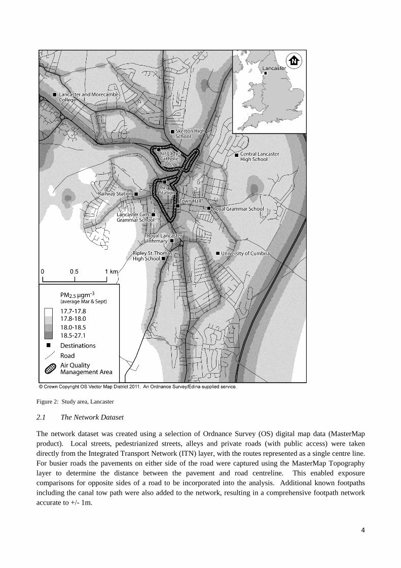
This case study focuses on the city of Lancaster, North West England, which has a population of approximately 55,000. While there are no major air pollution problems in Lancaster, an air quality management area has been declared around the main gyratory system where traffic congestion frequently occurs during peak hours – this is illustrated in Figure 2.

4

Figure 2: Study area, Lancaster

2.1 The Network Dataset

The network dataset was created using a selection of Ordnance Survey (OS) digital map data (MasterMap product). Local streets, pedestrianized streets, alleys and private roads (with public access) were taken directly from the Integrated Transport Network (ITN) layer, with the routes represented as a single centre line. For busier roads the pavements on either side of the road were captured using the MasterMap Topography layer to determine the distance between the pavement and road centreline. This enabled exposure comparisons for opposite sides of a road to be incorporated into the analysis. Additional known footpaths including the canal tow path were also added to the network, resulting in a comprehensive footpath network accurate to +/- 1m.

5

Where both sides of the road were captured separately, road crossing locations needed to be incorporated into the network. Google Street View was used to identify the location and type of pedestrian crossings on main roads within the study area. Additional crossing points were added at further locations where the provision of specified pedestrian crossing points was limited (as quiet local streets are represented by a single road centreline this assumes no time for crossing roads). For busier roads time impedances for crossing were assumed as listed in Table 1. The crossing impendences where estimated from field observation and information from the local authority regarding the phasing of traffic lights.

Table 1. Time impedance for crossing roads.

Crossing type Time impedance (seconds)

Traffic island Traffic island on busy road sections Zebra crossing Pedestrian lights Pedestrian lights as part of traffic control Additional crossing points Additional crossing points on busy road sections

For the purpose of this analysis a typical walking speed of 5kph was assumed (Colclough and Owens, 2010). The impact of gradient on walking speeds was also calculated. Directional-dependant slope was calculated for each segment of the network, first ensuring that no network segment was greater than 50m in length to reduce the likelihood of multiple changes in slope direction. Walking speeds were assigned to network segments as shown in Table 2 (Finnis and Walton, 2007 and Colclough and Owens, 2010)

Table 2. Variation in walking speed with slope

Gradient (◦) Uphill speed (km/h) Downhill speed (km/h) 0 - 4.5 5.0 5.0 4.5 - 6.5 5.5 5.7 6.5 - 7.5 5.0 5.2

> 7.5 4.6 4.7

2.2 Respiratory Minute Volume

Physiology and activity level are represented in the analysis through the calculation of Respiratory Minute Volume (VE). When combined with PM2.5 concentrations and duration of exposure, VE can be used to calculate exposure in terms of inhaled dose. VE is calculated for metabolic equivalents (MET) representing varying activity levels with slope, at the assumed walking speeds already defined. The METs were taken from the Ainsworth et al, 2011 and are summarised in Table 3.

6

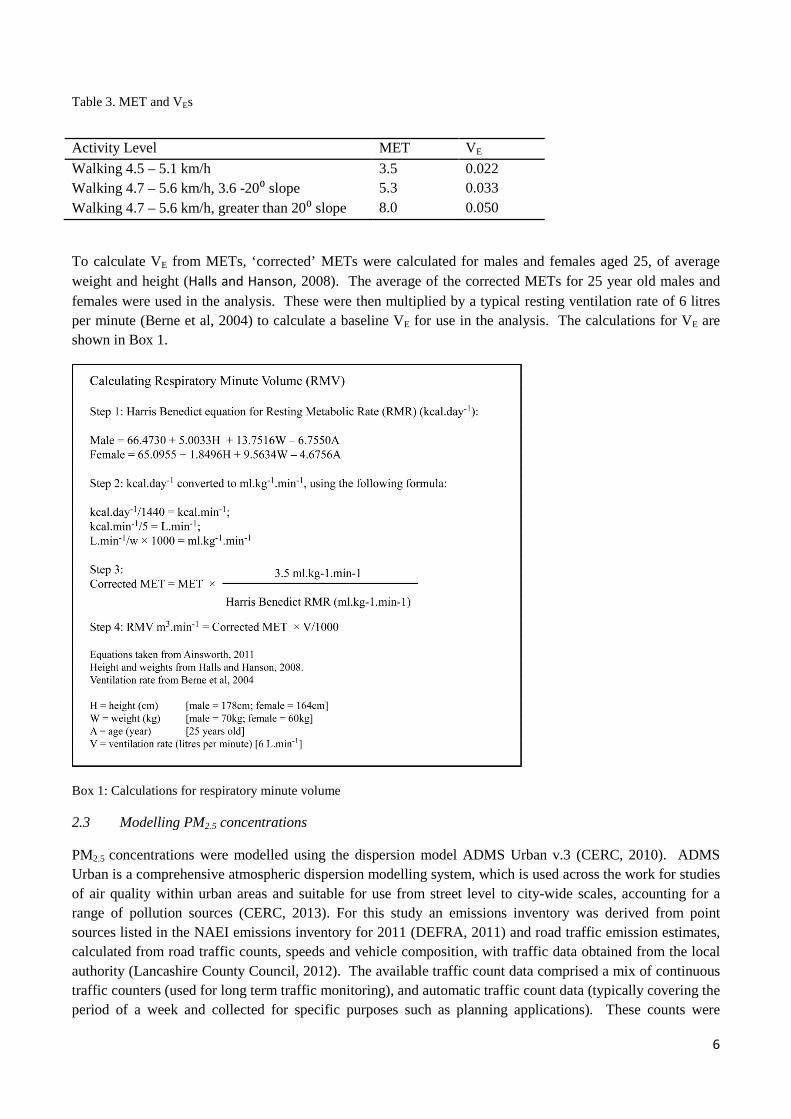
Table 3. MET and VEs

Activity Level MET VE Walking 4.5 – 5.1 km/h 3.5 0.022 Walking 4.7 – 5.6 km/h, 3.6 -20⁰ slope 5.3 0.033 Walking 4.7 – 5.6 km/h, greater than 20⁰ slope 8.0 0.050

To calculate VE from METs, ‘corrected’ METs were calculated for males and females aged 25, of average weight and height (Halls and Hanson, 2008). The average of the corrected METs for 25 year old males and females were used in the analysis. These were then multiplied by a typical resting ventilation rate of 6 litres per minute (Berne et al, 2004) to calculate a baseline VE for use in the analysis. The calculations for VE are shown in Box 1.

Box 1: Calculations for respiratory minute volume

2.3 Modelling PM2.5 concentrations

PM2.5 concentrations were modelled using the dispersion model ADMS Urban v.3 (CERC, 2010). ADMS Urban is a comprehensive atmospheric dispersion modelling system, which is used across the work for studies of air quality within urban areas and suitable for use from street level to city-wide scales, accounting for a range of pollution sources (CERC, 2013). For this study an emissions inventory was derived from point sources listed in the NAEI emissions inventory for 2011 (DEFRA, 2011) and road traffic emission estimates, calculated from road traffic counts, speeds and vehicle composition, with traffic data obtained from the local authority (Lancashire County Council, 2012). The available traffic count data comprised a mix of continuous traffic counters (used for long term traffic monitoring), and automatic traffic count data (typically covering the period of a week and collected for specific purposes such as planning applications). These counts were

7

supplemented where available with Annual Average Daily Flow (AADF) traffic counts (DFT, 2011). The dates for available data varied, with records chosen from the available data which most closely represented typical morning rush hour (08:00-09:00) for the year 2011. Traffic flow and composition data were assigned to road centrelines from the OS MasterMap ITN layer, which were then imported to ADMS-Urban to represent road sources. The latest road source emission factor dataset UK EFT v4.2 was utilized within the model (CERC, 2010). Canyons were modelled for sections of the main gyratory around the city centre, where the road is surrounded by tall buildings on either side. The canyon widths were measured from the MasterMap Topography layer, and heights for surrounding buildings calculated from LiDAR data.

Meteorological data were taken from Manchester Ringway meteorological station (BADC, 2012) (45 miles south east of Lancaster). Background PM2.5 data were obtained from DEFRA’s air quality data archive (http://uk-air.defra.gov.uk/data/) for the urban background monitoring site for Preston (20 miles south of Lancaster). Due to missing records, the months of March and September were taken as being broadly representative of the range of meteorological conditions experienced throughout 2011.

The model was run to a set of 234,563 receptors spaced at 2m intervals along each line segment in the network. The average PM2.5 concentration per line segment was subsequently calculated for the period 08:00 to 09:00 hours and assigned to each line segment in the path network.

2.4 Exposure Calculation

Slope for each line segment was calculated from the length of the line segment and the difference in elevation between its start and end points. For both uphill and downhill directions the duration in minutes was calculated from the length and the appropriate speed as defined earlier in Table 2. Appropriate VE rates were also assigned to uphill and downhill directions for each line segment relative to the slope. From these attributes exposure to PM2.5 in both uphill and downhill directions was calculated for every line segment in the path network based on the equation:

Exposure (µg) = Mean PM2.5 (µg.m-3) × Duration (minutes) × VE (m3.min-1)

2.5 Network Analysis

Network analysis was carried out using the network analyst extension within ArcGIS 10 (ESRI, 2010) Network attributes were created both for the duration in minutes and the exposure to PM2.5 for each of the 60 sample days in the study. This enables either fastest, or least polluted routes to be computed from any origin to any destination within the study area on any given day. For each route the accumulated time and PM2.5 exposure is calculated.

In addition to calculating individual routes, Origin Destination (OD) cost matrixes were used to compute journey time exposure for numerous routes throughout the city, from each postcode centroid (which typically represents around 15 addresses (ONS, 2012)), to a set of 12 destinations shown in Figure 2, which represent the main secondary and tertiary education providers, key employers such as the city council and hospital, and the major public transport hubs within the city. OD cost matrixes are used to compute and store the fastest or least polluted path between multiple combinations of potential route Origins (start points) and Destinations (end points). While OD cost matrices do not display the routes chosen they are able to generate accumulated PM2.5 exposure for hundreds of potential routes, limited only by the number of Origins and Destinations required and the size and quality of the network dataset. They therefore enable a broader analysis of the variation in potential journey-time exposure across the city.

8

The analysis was run first to demonstrate its application in assessing journey time exposure, assuming fastest routes between origin and destination were chosen. Routes designed to minimise exposure to PM2.5 were also generated.

3 Case Study Results

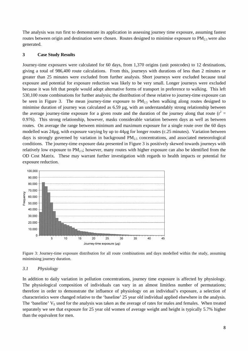
Journey-time exposures were calculated for 60 days, from 1,370 origins (unit postcodes) to 12 destinations, giving a total of 986,400 route calculations. From this, journeys with durations of less than 2 minutes or greater than 25 minutes were excluded from further analysis. Short journeys were excluded because total exposure and potential for exposure reduction was likely to be very small. Longer journeys were excluded because it was felt that people would adopt alternative forms of transport in preference to walking. This left 530,100 route combinations for further analysis; the distribution of these relative to journey-time exposure can be seen in Figure 3. The mean journey-time exposure to PM2.5 when walking along routes designed to minimise duration of journey was calculated as 6.59 µg, with an understandably strong relationship between the average journey-time exposure for a given route and the duration of the journey along that route (r2 = 0.976). This strong relationship, however, masks considerable variation between days as well as between routes. On average the range between minimum and maximum exposure for a single route over the 60 days modelled was 24µg, with exposure varying by up to 44µg for longer routes (c.25 minutes). Variation between days is strongly governed by variation in background PM2.5 concentrations, and associated meteorological conditions. The journey-time exposure data presented in Figure 3 is positively skewed towards journeys with relatively low exposure to PM2.5; however, many routes with higher exposure can also be identified from the OD Cost Matrix. These may warrant further investigation with regards to health impacts or potential for exposure reduction.

Figure 3: Journey-time exposure distribution for all route combinations and days modelled within the study, assuming minimising journey duration.

3.1 Physiology

In addition to daily variation in pollution concentrations, journey time exposure is affected by physiology. The physiological composition of individuals can vary in an almost limitless number of permutations; therefore in order to demonstrate the influence of physiology on an individual’s exposure, a selection of characteristics were changed relative to the ‘baseline’ 25 year old individual applied elsewhere in the analysis. The ‘baseline’ VE used for the analysis was taken as the average of rates for males and females. When treated separately we see that exposure for 25 year old women of average weight and height is typically 5.7% higher than the equivalent for men.

9

The impact of changes in weight and height were explored relative to a 25 year old male, 178cm tall and weighing 70kg and are shown in Table 4. As age increases it can be seen that exposure increases by approximately 4% per decade. Furthermore, the results show that being overweight can significantly increase journey-time exposure to air pollution.

Table 4: Percentage difference in exposure with changes in age and height. Difference measured from a base case of a 25 year old male, 178cm tall and 70kg.

Male 178cm tall

Weight (kg)

60 70 80 90 100

Age

15 -10.7 -3.7 2.3 7.5 12.1

25 -7.0 0.0 6.0 11.1 15.6

35 -2.9 4.0 9.9 14.9 19.3

45 1.5 8.4 14.1 19.1 23.3

55 6.4 13.1 18.7 23.5 27.6

65 11.7 18.2 23.7 28.2 32.1

3.2 Speed

The speed at which an individual walks (or runs) during their journey affects their journey-time exposure by influencing both the duration of the journey and their respiratory minute volume. Calculating VE from METs associated with a range of walking and running speeds (Ainsworth et al, 2011) enables us to assess the impact on journey-time exposure. As speed increases so does physical activity and therefore VE, whilst journey duration decreases. Figure 4 compares the baseline, moderate walking speed (5kph), with a range of other speeds. From this we can conclude that a moderate walking speed is the optimum for minimising journey-time exposure. At slower speeds the balance between reduced ventilation rate and increased duration leads to slightly increased exposure. At faster speeds the increased VE associated with walking briskly or running fails to be sufficiently offset by reductions in journey duration and therefore leads to significant increases in exposure. Similar patterns with optimum speeds for exposure reduction have been observed by Int Panis et al (2011) when monitoring exposure of cyclists in Belgium.

Figure 4. Differences in exposure with changes in speed.

10

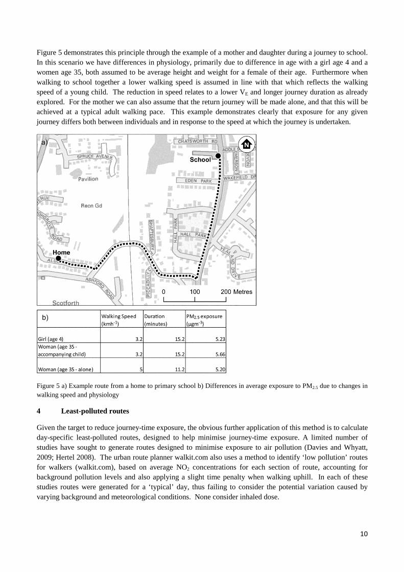
Figure 5 demonstrates this principle through the example of a mother and daughter during a journey to school. In this scenario we have differences in physiology, primarily due to difference in age with a girl age 4 and a women age 35, both assumed to be average height and weight for a female of their age. Furthermore when walking to school together a lower walking speed is assumed in line with that which reflects the walking speed of a young child. The reduction in speed relates to a lower VE and longer journey duration as already explored. For the mother we can also assume that the return journey will be made alone, and that this will be achieved at a typical adult walking pace. This example demonstrates clearly that exposure for any given journey differs both between individuals and in response to the speed at which the journey is undertaken.

Figure 5 a) Example route from a home to primary school b) Differences in average exposure to PM2.5 due to changes in walking speed and physiology

4 Least-polluted routes

Given the target to reduce journey-time exposure, the obvious further application of this method is to calculate day-specific least-polluted routes, designed to help minimise journey-time exposure. A limited number of studies have sought to generate routes designed to minimise exposure to air pollution (Davies and Whyatt, 2009; Hertel 2008). The urban route planner walkit.com also uses a method to identify ‘low pollution’ routes for walkers (walkit.com), based on average NO2 concentrations for each section of route, accounting for background pollution levels and also applying a slight time penalty when walking uphill. In each of these studies routes were generated for a ‘typical’ day, thus failing to consider the potential variation caused by varying background and meteorological conditions. None consider inhaled dose.

11

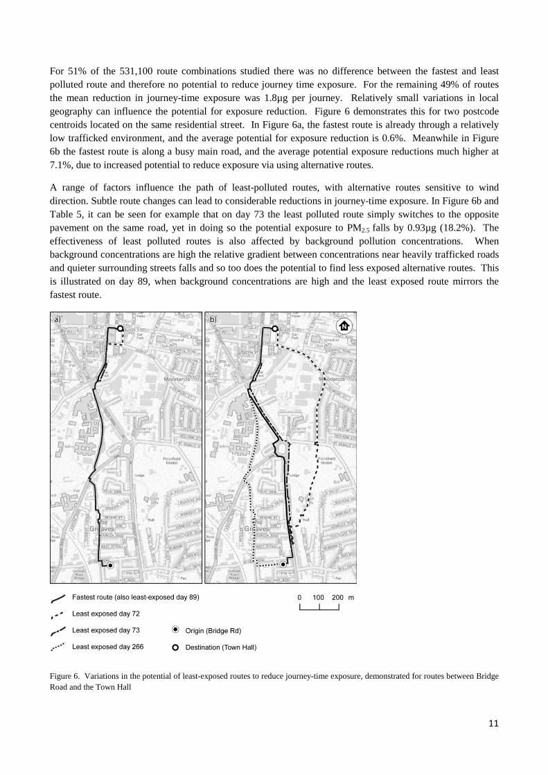
For 51% of the 531,100 route combinations studied there was no difference between the fastest and least polluted route and therefore no potential to reduce journey time exposure. For the remaining 49% of routes the mean reduction in journey-time exposure was 1.8µg per journey. Relatively small variations in local geography can influence the potential for exposure reduction. Figure 6 demonstrates this for two postcode centroids located on the same residential street. In Figure 6a, the fastest route is already through a relatively low trafficked environment, and the average potential for exposure reduction is 0.6%. Meanwhile in Figure 6b the fastest route is along a busy main road, and the average potential exposure reductions much higher at 7.1%, due to increased potential to reduce exposure via using alternative routes.

A range of factors influence the path of least-polluted routes, with alternative routes sensitive to wind direction. Subtle route changes can lead to considerable reductions in journey-time exposure. In Figure 6b and Table 5, it can be seen for example that on day 73 the least polluted route simply switches to the opposite pavement on the same road, yet in doing so the potential exposure to PM2.5 falls by 0.93µg (18.2%). The effectiveness of least polluted routes is also affected by background pollution concentrations. When background concentrations are high the relative gradient between concentrations near heavily trafficked roads and quieter surrounding streets falls and so too does the potential to find less exposed alternative routes. This is illustrated on day 89, when background concentrations are high and the least exposed route mirrors the fastest route.

Figure 6. Variations in the potential of least-exposed routes to reduce journey-time exposure, demonstrated for routes between Bridge Road and the Town Hall

12

Table 5. Examples of journey-time exposure reductions for routes in Figure 6b with corresponding background and wind conditions.

Route Time* (min)

Fastest route (µg)

Least exposed route (µg)

Reduction (µg)

Reduction (%)

Back-ground PM2.5

(µg.m-3)

Wind direction (o)

Wind speed ms-1

Day 72 18.9 2.55 2.17 0.38 14.9 4 270 2.1 Day 73 17.5 5.12 4.19 0.93 18.2 9 60 1.5 Day 89 17.0 21.18 21.18 0.00 0.0 53 180 4.1 Day 266 18.1 6.20 5.94 0.26 4.2 14 180 4.1 * Time for least exposed route. The time for the fastest route in Figure 6b is 17.0 minutes.

While the results demonstrate only small average reductions in exposure, the benefits of any reduction to PM2.5 will be cumulative over many months and years. The analysis presented here specifically looks to address ways in which to reduce journey-time exposure when commuting, for which an individual may be assumed to make in the region of 225 return trips per year. For example between the example at the top of Bridge Road and the Town Hall shown in Figure 6b, the average potential reduction in exposure resulting from walking a least exposed route is 0.36µg would result in a reduction in inhaled PM2.5 of 162µg per year. As PM2.5 is a non-threshold pollutant, even small reductions in pollution may have potential health benefits (RCEP, 2007; Pope and Dockery, 2006).

5 Discussion and Conclusion

The method presented facilitates analysis of a wide range of factors influencing journey-time exposure, as outlined in Figure 1, providing the potential for more accurate journey-time exposure assessments for epidemiological studies. In considering ways to reduce exposure to PM2.5 it also provides a means with which to assess the trade-off between activity level and duration; the potential benefits of choosing alternative routes; and the influence of other factors such as weight on journey-time exposure. The spatial resolution of the method enables variations in the exposure of individuals to be assessed in more detail than using pollution concentrations from a central monitoring site. The method has the potential to be expanded to link together multiple journey-time exposure estimates with pollution estimates for fixed locations (e.g. home or work) where people spend time between periods of transit, thus providing a modelled alternative to the time-activity patters and exposure calculations carried out through monitoring in studies such as Dons et al (2012).

While recognising that all models are necessarily limited in the extent to which they are able to represent the real world, or a given individual, this method adds to current approaches by incorporating activity level and physiology into the modelling of journey-time exposure. There remain, however, specific factors that this approach is unable to address, for example variations in the health and fitness of an individual. The model presented here links VE to path segments based upon their slope, but fails to account for the influence the slope of previous segments may have on VE as there each segment may potentially be reached from a number of different directions.

The method is scalable and can potentially be applied wherever path information exists and traffic flow can be estimated. Within the case study presented traffic flow information was the least adaptable element of the analysis, with considerable time required to derive information from a variety of traffic count data. For study areas with established traffic flow models this information should be easier to process and may enable greater flexibility to model different times of day, or year. While the case study presented successfully demonstrates the method for pedestrians only, the same principles could easily be applied to any mode of transport and to

13

multimodal networks. Exploring differences between transport mode will require consideration of a greater variety of activity levels and associated metabolic equivalents. Relationships between indoor and outdoor pollutant concentrations also need to be considered for some transport modes, although there is currently limited consensus regarding the scaling of pollutant concentrations (Boogard et al, 2009; Briggs et al, 2008; Esber et al, 2007; Int Panis 2010; Kaur et al, 2007; Yu et al, 2012; Zuurbier et al, 2010). Running the model for a specific day requires the availability of both meteorological data and background concentrations, for which missing records often exist. Of all steps in the method, assigning average pollution concentrations to network segments was the most processing intensive, due to the fine scale (2m spaced receptors) at which the model was run. This fine scale, however, is important if subtle differences, such as the difference between sides of the road (typically 8-10m wide) are to be explored.

It is acknowledged that there is limited available data against which to validate the current model. Neither of the local air quality monitoring sites within Lancaster monitor PM2.5 and both are situated in unrepresentative areas (next to the bus station and next to a feeder lane at a busy junction); hence these are not suitable for validation purposes. VE calculations were compared against inhalation rates reported by the USEPA (2011) and found to be in line with these calculations.

Using the method to identified routes of least exposure through the network, it is clear that the potential for reducing exposure varies greatly between days, depending on background concentrations and meteorology, especially wind direction and wind speed. The effective design of least polluted routes, therefore, needs to reflect daily variations rather than ‘average’ conditions. In exploring least polluted routes the sensitivities of pavement choice identified by Kaur et al (2005) and Greaves (2008) were also confirmed, with significant reductions in exposure being seen in some cases by simply crossing the road.

In conclusion, the methodology presented builds on existing published work, by enabling physiology and activity level to be incorporated into a modelling approach. The flexibility and scalability of the approach offer potential to explore fully the interactions between physiology, activity level, journey duration and pollution concentrations. With the ability to compute calculations for multiple sets of background and meteorological conditions, to tailor to an individual’s physiology and to expand the approach to consider multiple transport modes the method provides a means for calculating more accurate exposure estimates for individuals or cohorts which has potential benefits for future epidemiological studies exploring the impact of air pollution on human health.

Acknowledgements We would like to thank Lancashire County Council for providing traffic count data, which was essential to this study, and the reviewers of this paper for their constructive comments. References Ainsworth BE, Haskell WL, Herrmann SD, Meckes N, Bassett Jr DR, Tudor-Locke C, et al. The Compendium of

Physical Activities Tracking Guide. Healthy Lifestyles Research Center, College of Nursing & Health Innovation, Arizona State University. https://sites.google.com/site/compendiumofphysicalactivities/home. Accessed10/12/12

British Atmospheric Data Centre (BADC) 2012 http://badc.nerc.ac.uk/home/index.html Accessed 07/11/12. Berne RM, Levy MN, Koeppen BM, Stanton BA. Physiology. 5th ed. Missouri: Mosby; 2004. Boogard H, Borgman F, Kamminga J, Hoek G. Exposure to ultrafine and fine particles and noise during cycling and

driving in 11 Dutch cities. Atmospheric Environment. 2009; 43:4234-4242. Briggs D. The Role of GIS: Coping With Space (And Time) in Air Pollution Exposure Assessment. Journal of

Toxicology and Environmental Health: Part A 2005; 68:1243-1261.

14

Briggs D, de Hoogh K, Morris C, Gulliver J. Effects of travel mode on exposure to particulate air pollution. Environment International. 2008; 34:12-22.

Cambridge Environmental Research Consultants (CERC). ADMS-Urban 3. 2010. Cambridge. Cambridge Environmental Research Consultants (CERC). ADMS-Urban User Guide. 2013. Cambridge.

http://www.cerc.co.uk/environmental-software/assets/data/doc_userguides/CERC_ADMS-Urban3.2_User_Guide.pdf. Accessed 11/12/13.

Chan LY, Lau WL, Zou SC, Cao ZX, Lai SC. Exposure level of carbon monoxide and respirable suspended particulate in public transportation modes while commuting in urban area of Guangzhou, China. Atmospheric Environment 2002; 36:5831-5840.

Colclough J, Owens E. Mapping pedestrian journey times using a network-based GIS model. Journal of Maps 2010; 230-239.

Davies G, Whyatt JD. A least-cost approach to personal exposure reduction. Transactions in GIS 2009; 13(2): 229-246. de Hartog J, Boogard H, Nijland H, Hoek G. Do the health benefits of cycling outweigh the risk? Environmental Heath

Perspectives. 2010; 118(8): 1109-1116. Department for Environment, Food and Rural Affairs (DEFRA) 2011. National Atmospheric Emissions Inventory

http://naei.defra.gov.uk/ Accessed 8/11/12. Department for Transport (DFT). Traffic Counts. http://www.dft.gov.uk/traffic-counts. 2011. Accessed 15/11/12 Dons E, Temmerman P, Van Poppel M, Bellemans T, Wets G, Int Panis L. Street characteristics and traffic factors

determining road user’ exposure to black carbon. Science of the Total Environment 2013; 447: 72-79. Dons E, Int Panis L, Van Poppel M, Theunis J, Wets G. Personal exposure to Black Carbon in transport

microenvironments. Atmospheric Environment 2012; 55:392-398. ESRI (2010). ArcGIS Desktop 10. Redlands, California. Finnis K, Walton D. Field observations to determine the influence of population size, location and individual factors on

pedestrian walking speeds. Ergonomics 2007; 51(6): 827-742 Gómez-Perales JE, Colvile RN, Nieuwenhuijsen M.J, Fernandez-Bremauntz A, Gutierrez F, Bernabe-Cabanillas R et al.

Commuters’ exposure to PM2.5, CO, and benzene in public transport in the metropolitan area of Mexico City. Atmospheric Environment 2004; 38(8): 1219-1229.

Greaves S, Issarayangyun T, Liu Q. Exploring variability in pedestrian exposure to fine particulates (PM2.5) along a busy road. Atmospheric Environment 2008; 42: 1665-1676.

Gulliver J, Briggs DJ. Time-space modelling of journey-time exposure to traffic-related air pollution using GIS. Environmental Research 2005; 97: 10-25.

Halls S, Hanson J. Heath calculators and charts. 2011. http://www.halls.md/ Accessed 10/12/12. Heinrich J, Schwarze PE, Stilianakis N, Momas I, Medina S, Totlandsdal AI et al. Studies on health effects of transport-

related air pollution. In: Health effects of transport-related air pollution. Krzyzanowski M, Kuna-Dibbert B, Schneider J. Denmark: World Health Organisation; 2005. p 25-65.

Hertel O, Hvidberg M, Ketzel M, Storm L, Stausgaard L. A proper choice of route significantly reduces air pollution exposure - A study on bicycle and bus trips in urban streets. Science of the Total Environment 2008; 389(1): 58-70.

Int Panis L, Meeusen R, Thomas I, de Geus B, Vandenbulcke-Passchaert G, Degraeuwe B, et al. Systematic analysis of Health risks and physical Activity associated with cycling Policies SHAPES-Final Report. Brussels: Belgian Science Policy. 2011; 20: 78–81

Int Panis L, de Geus B, Vandenbulcke G, Willems H, Degraeuwe B, Bleux N et al. Exposure to particulate matter in traffic: A comparison of cyclists and car passengers. Atmospheric Environment 2010; 44(19): 2263-2270.

Kaur S, Nieuwenhuijsen M, Colvile R. Personal exposure of street canyon intersection users to PM2.5, ultrafine particle counts and carbon monoxide in Central London, UK. Atmospheric Environment. 2005; 39: 3629-3641.

Kaur S, Nieuwenhuijsen M, Colvile R. Fine particulate matter and carbon monoxide exposure concentrations in urban street transport microenvironments. Atmospheric Environment. 2007; 41: 4781-4810.

Kousa A, Kukkonen J, Karppinen A, Aarnio P, Koskentalo T. A model for evaluating the population exposure to ambient air pollution in an urban area. Atmospheric Environment 2002; 36(13): 2109.

Krzyzanowski M. Health Effects of transport-related air pollution: summary for policy makers. 2005. World Health Organisation, Denmark.

Künzli N, Kaiser R, Medina S, Studnicka M, Chanel O, Filliger P, et al. Public-health impact of outdoor and traffic-related air pollution: a European assessment. The Lancet. 2000; 356(9232): 795-801.

15

McCreanor J, Cullinan P, Nieuwenhuijsen M, Stewart-Evans J, Malliarou E, Jarup L et al. Respiratory effects of exposure to diesel traffic in persons with asthma. 2007; 357(23):2348-2358.

Pedersen M, Giorgis-Allemand L, Bernard C, Aguilera I, Andersen A, Ballester F et al. Ambient air pollution and low birthweight: a European cohort study (ESCAPE). The Lancet Respiratory Medicine. 2013 In Press.

Peters A, von Klot S, Heier M, Trentinaglia I, Hormann A, Wichmann E, Lowel H. Exposure to Traffic and the Onset of Myocardial Infraction. The New England Journal of Medicine. 2004; 351(17): 1721-1730.

Pope CA, Dockery DW. Health Effects of Fine Particulate Air Pollution: Lines that Connect. Journal of the Air and Waste Management Association 2006; 56: 709-742.

Royal Commission on Environmental Pollution (RCEP). The Urban Environment, Royal Commission on Environmental Pollution 26th Report 2007; pages 35-40.

Schwartz J, Neas LM. Fine Particles Are More Strongly Associated than Coarse Particles with Acute Respiratory Health Effects in Schoolchildren. Epidemiology. 2000; 11(1): 6-10

United States Environmental Protection Agency (USEPA). Exposure Factors Handbook: 2011 Edition. www.epa.gov/ncea/efh/pdfs/efh_complete.pdf. Accessed 01/05/13.

walkit.com (2013). The Urban Walking Route Planner. walkit.com Accessed 04/01/2013, 2013 Xia Y, Tong H. Cumulative effects of air pollution on public health. Statistics in Medicine. 2006; 25: 3548-3559. Yu Q, Lu Y, Xiao S, Shen J, Li X, Ma W, Chen L. Commuters' exposure to PM1 by common travel modes in Shanghai.

Atmospheric Environment. 2012; 59: 39-46. Zuurbier M, Hoek G, Oldenwening M, Lenters V, Meliefste K, van den Hazel P, Brunekreef B. Commuters’ exposure to

particulate matter air pollution is affected by mode of transport, file type and route. Environmental Health Perspectives. 2010; 118(6):783-789.