A Neoclassical Kaldor Model of Real Wage

Declines

Michael Sattinger∗

Department of Economics

University at Albany

Albany, NY 12222, USA

Email m.sattinger@albany.edu

Phone: (518) 442-4761

JEL: D33, E12, H23, J31

Keywords: Kaldor, real wage, national debt, taxes

March 25, 2004

∗The author is indebted to Ken Beauchemin, Betty Daniel, Martin Gervais, Joop Har-tog, Michael Jerison, John Jones, Terry Kinal, Shannon Seitz, Peter Skott, Coen Teulingsand participants at seminars at the University at Albany, Queens University, and AarhusUniversity for helpful comments. An alternative version of this paper, using a matchingtechnology, was presented at the conference “On the Wealth of Nations — Extending theTinbergen Heritage,” at Erasmus University. The author acknowledges support from theInstitute for the Study of Labor (IZA) during the initial stages of this research. Errorsand opinions are the responsibility of the author.

1

Abstract

A model linking macroeconomic equilibrium and income distrib-

ution in balanced growth equilibria is developed as a variant to the

Kaldor model of factor shares. It departs from the original Kaldor

model in assuming equal saving rates and a neoclassical production

function. Macroeconomic equilibrium (national savings equal to in-

vestment) combines with competitive microeconomic behavior to de-

termine the real wage and real interest rate. An increase in the ratio

of national debt to labour reduces the real wage, explaining recent

declines.

1 Introduction

The U.S. economy in past decades has exhibited a substantial decline in the

real wage relative to productivity and large changes in the real interest rate

over long periods. This paper develops a model linking macroeconomic policy

variables to factor prices and income distribution. Macroeconomic equilib-

rium (Aggregate Demand equal to Aggregate Supply, or national savings

equal to investment) determines a relationship between the real interest rate

and the ratio of capital to labor. Microeconomic equilibrium, arising from

competitive generation of factor prices, determines a second relationship be-

tween the two variables. Together, macroeconomic and microeconomic equi-

librium determine the real interest rate, the capital to labor ratio, and the

real wage rate in balanced growth.

2

The model developed is a variant of Nicholas Kaldor’s Keynesian model

of income distribution (1955-1956, 1957), in which equality between savings

and investment is brought about by shifts between profit and labor income in-

stead of by fluctuations in economic activity.1 In Kaldor’s approach, income

distribution is partly explained by macroeconomic phenomena, and shifts

of factor incomes are necessary to bring about macroeconomic equilibrium.

The model developed here shares with Kaldor’s model the involvement of

income distribution with macroeconomics and the simultaneous explanation

of both distributional and macroeconomic phenomena. However, the mecha-

nism linking macroeconomic equilibrium and income distribution is different.

In Kaldor’s model, full employment is assumed and an aggregate investment

rate is determined exogenously by balanced growth parameters. With a

greater saving rate out of profits, income shifts between profits and labor in-

come are brought about by changes in prices relative to wage rates until the

aggregate saving rate equals the required investment rate. In contrast, in the

model developed here, the level of production is determined endogenously,

and the saving rate is assumed to be the same for all sources of income. All

variables are real, so there is no inflation to bring about changes in the wage

rate relative to the price level. In Kaldor’s model, there is a fixed capital

1See discussions of Kaldor’s model in G. Bertola (2000, pp. 400-498), C.E. Ferguson(1969, pp. 314-322), Mitsuhiko Iyoda (1997), Luigi Pasinetti (1962), Kurt Rothschild(1993, Chapters 17-19), Sattinger (2001, pp. liii-liv), Peter Skott (1989a, 1989b), andJames Tobin (1989). Kaldor’s model is one of several approaches that involve incomedistribution in a macroeconomic model (see Bertola, 2000, Sattinger, 1990, and SydneyWeintraub, 1958). Per Krusell and Anthony Smith (1999) consider distributional impactsamong heterogeneous asset levels of eliminating business cycles.

3

to production ratio so that marginal products of factors are not defined and

play no role in determining factor prices. In the model developed here, a neo-

classical production function relates marginal products of capital and labor

to the ratio of capital to labor. Use of a neoclassical production function is

intended to counter the argument that factor non-substitutability generates

the results.

Table 1 shows interest rate, wage and debt variables that are relevant in

this paper. The data are for the U.S. in the period 1961 to 1999. The real

interest rate in Column 2 is measured by the average interest rate on U.S.

Treasury bonds with maturity over ten years minus inflation as measured

by increases in the yearly average Consumer Price Index (CPI-U). The real

wage is measured by average hourly earnings in 1982 dollars for total private

employment, not seasonally adjusted. Column 4 is the real wage from Col-

umn 3 divided by productivity as measured by the Major Sector Multifactor

Productivity Index for manufacturing (times 100). Column 5 shows the ratio

of national debt to output, from the 2003 Economic Report of the President,

measured as the ratio of national debt held by the public to Gross Domestic

Product. The series can be regarded as national debt per employed worker,

divided by output per employed worker. It is then national debt per employed

worker controlling for productivity changes. Column 6 shows the saving rate

measured in the National Income and Product Accounts by personal savings

as a percentage of personal income. There are alternative ways of measuring

4

these variables, but the major patterns are unlikely to be affected.2

The data show substantial changes in factor prices over long periods of

time, with no indication that they are returning to an earlier equilibrium

level. The real interest rate lies between two and three percent in the first

half of the 1960’s, falls below one percent (and often goes negative) from

1973 to 1980, rises to between five to eight percent between 1982 and 1987,

and falls back to a range of three to five percent from 1988 on. As the real

interest rate falls, the real wage rises from below seven in 1961 to levels above

eight from 1970 to 1979. Then as the real interest rate rises from below one

percent to above 3 percent for a 17 year period, the real wage falls to a level

below 8.3 The real wage decline relative to productivity cannot be explained

by increases in benefits from 1980 to 1999, the period for which data are

available from the U.S. Bureau of Labor Statistics. In that period, total

compensation for total private employment (including wages, salaries and

benefits) divided by multifactor productivity declined by 18 percent.

These changes are not an outcome of business cycle models describing

fluctuations around a long run equilibrium. The long run changes in the real

interest rate and wage rate could potentially be explained by the episode

of inflation in the 1960’s and 1970’s but only by abandoning views that the

2See Alan Kreuger, 1999, for discussion of measurement problems.3R. Blundell and T. MacCurdy (1999, pp. 1583-1586) analyze real wage rates over

time by educational level and gender. In the U.S., real wages declined for men but not forwomen over long periods. Real wages did not decline in the United Kingdom or Germanyover the same periods. Lawrence F. Katz and David H. Autor (1999, p. 1476) also showreal wage declines from 1971 to 1995 based on Current Population Survey data.

5

effects of inflation on factor prices end less than a decade after stabilization

of monetary growth. Productivity also does not explain the long run and

substantial changes. Increases in productivity should raise both the real

interest rate and the real wage. However, the real wage declines relative to

multifactor productivity, as shown in the ratio in Column 4, from 1978 on.

Use of output per hour instead of multifactor productivity would result in

even steeper declines in the ratio of wages to productivity. Imperfections in

the measurement of productivity cannot be the explanation for the observed

long run behavior of factor prices since real interest rates and real wages

move in opposite directions. Other explanations are possible (e.g., capital-

skill complementarity) and cannot be ruled out by these data.

This paper proposes an explanation based on the link between the macro-

economic sector and microeconomic determination of factor prices. The styl-

ized facts concerning long run relationships to be addressed by the model

developed here are as follows. Over the period 1961 to 1999, the real interest

rate declines, increases substantially and then declines to a level greater than

at the start of the period. The real wage relative to productivity is roughly

inversely related to the real interest rate, rising and then declining. These

patterns occur contemporaneously with a decline in the ratio of national debt

to output from 1961 to the 1970’s, followed by increases. While the short

run effect of budget deficits on the interest rate are well known, this paper

focuses on the ratio of national debt to output in balanced growth and its ef-

fects on both the real interest rate and the real wage rate. In the model that

6

will be developed, balanced growth of a greater national debt absorbs more

savings, raising the interest rate at each capital to labor ratio. In balanced

growth equilibrium, greater national debt per worker then yields a higher

real interest rate and a lower real wage rate.

The model developed here is referred to as the neoclassical Kaldor model

to distinguish it from the original Kaldor model with unequal saving rates.

The economy is essentially Non-Ricardian since new entrants do not neces-

sarily have the same asset levels as individuals who entered earlier. There

are two forms of income: labor income from wages (plus transfers from the

government) and interest from ownership of either capital or national debt.

Microeconomic and macroeconomic policies are incorporated in the form of

tax rates on labor and interest income, a tax rate on output (a value added

tax), and the ratio of national (government) debt to employment. For sim-

plification, only a closed economy is considered, and there is no inflation or

technological change. The population grows at a constant rate.

Balanced growth equilibrium will be determined from microeconomic and

macroeconomic equilibrium conditions relating the (real) interest rate to the

capital to labor ratio. Section 2 derives in a straightforward way the condition

for microeconomic equilibrium. Section 3 develops conditions for macroeco-

nomic equilibrium. The saving behavior of households is a standard solution

to an optimal control problem. From the government balanced growth bud-

get constraint and the expression for taxes, it is possible to solve for the level

of transfers at which the government budget constraint is satisfied. The con-

7

dition for macroeconomic equilibrium can then be determined from setting

Aggregate Demand equal to Aggregate Supply, after substituting the expres-

sions for taxes and transfers. Section 4 describes balanced growth equilib-

rium, which arises when both microeconomic and macroeconomic equilibrium

conditions are satisfied. Sections 5 and 6 derive the effects of macroeconomic

and microeconomic policies, respectively. Section 7 considers alternative sav-

ing behavior that would eliminate effects of macroeconomic policies on factor

prices. It also relates the results to current macroeconomic analysis. Section

8 considers whether the current model meets previous criticisms of Kaldor’s

model. It also describes extensions to the model.

2 Microeconomic Equilibrium

The microeconomic equilibrium condition arises from a neoclassical produc-

tion function relating output to amounts of capital and labor. Let f [K,L]

be the rate of output generated using K units of capital and L units of la-

bor. Assume f [K,L] is homogeneous of degree one, has continuous first and

second partial derivatives, and has a diminishing marginal rate of technical

substitution in the substitution region. Let fL = ∂f/∂L and fK = ∂f/∂K

be the marginal products. Assume the price of output is normalized to be 1.

Let tp be the tax rate on output (equivalent to a value added tax), the same

for all firms and all levels of output. Let r and w be the real interest and

wage rates, respectively, and assume r and w are taken as given by firms.

8

An individual firm’s rate of profits, π, is

π = (1− tp)f [K,L]− rK − wL (1)

The firm’s first order conditions for profit maximization are

r = (1− tp)fK (2)

w = (1− tp)fL (3)

The microeconomic equilibrium condition arises directly from the firm’s first

order conditions assuming all firms have the same production function. Since

f is homogeneous of degree one, fK and fL are homogeneous of degree zero,

i.e. they are functions of K/L. Let κ[r] be the capital to labor ratio that

solves the first order condition 2. The microeconomic equilibrium condition

is then:

K/L = κ[r] (4)

Since the marginal product of capital is a declining function of K/L, the

capital to labor ratio is a decreasing function of the interest rate in the micro-

economic equilibrium condition. Given κ[r], the wage w can be determined

from the first order condition 3.

Individuals participate in the labor force when the after tax wage rate

exceeds the opportunity cost of their time. Let tw be the tax rate on labor

income, the same for all individuals and all levels of income. Let λ[(1− tw)w]

9

be the proportion of individuals working when the after tax wage rate is

(1− tw)w. Suppose the population grows at a constant rate ρ and let N0eρt

be the population size at time t. The labor supply at time t is then

λ[(1− tw)w]N0eρt (5)

At a given wage rate, the labor supply grows at the rate ρ.

The sequence of determination in the microeconomic sector is that the

interest rate determines the capital to labor ratio through the microeconomic

condition κ[r]. Then the capital to labor ratio determines the wage rate from

the first order condition for labor, and the wage rate determines labor supply

through λ[(1− tw)w]N0eρt.

3 Macroeconomic Equilibrium

3.1 Assumptions

The macroeconomic equilibrium condition is determined in two steps. Opti-

mal intertemporal behavior determines the relation between the saving rate

and the real interest rate, and Aggregate Demand equal to Aggregate Sup-

ply determines the relation between the saving rate and the capital to labor

ratio. There are two types of income in the economy. Labor income consists

of labor earnings plus government transfers, wL+R, where R is government

transfers to individuals. Interest income consists of interest on capital and

10

on national debt, r(K +D), where D is national (government) debt.

The government taxes labor and interest income at potentially different

tax rates, pays interest at rate r on the national debt, expands the national

debt at the balanced growth rate ρ, and distributes the residual in the form of

transfers to individuals in the economy. Since only balanced growth equilibria

are compared, deficits or surpluses beyond balanced growth expansion cannot

occur. Total taxes in the economy are given by

T = tw(wL+R) + trr(K +D) + tpf [K,L] (6)

The government’s budget constraint can be expressed as

T + ρD = rD +R (7)

where the left side is government sources of funds and the right side is uses of

funds. In balanced growth, T, D and R increase at the rate ρ, so the budget

constraint remains satisfied at all times. Substituting T from 6 into 7 and

solving for R yields

R =1

1− tw(twwL+ trr(K +D) + tpf [K,L] + (ρ− r)D) (8)

When this expression is used for R in Aggregate Demand, the government

budget constraint is automatically satisfied.

Using r to discount future amounts, the present discounted value of na-

11

tional debt at time τ in the future for a balanced growth equilibrium is

D0eρτe−rτ , where D0 is current government debt. If r > ρ, this present

discounted value approaches zero, satisfying the no-Ponzi-game condition

(Olivier J. Blanchard and Stanley Fischer, 1989, p. 127). Even if r < ρ,

the present discounted value of the ratio of national debt to employment

approaches zero.

3.2 The Saving Rate

In this section, intertemporal optimization generates a relation between sav-

ings and the interest rate. Although the neoclassical Kaldor model can be

worked out for an arbitrary savings function, a relation consistent with in-

tertemporal optimization will demonstrate that the results are not generated

by departures from optimizing behavior.

Consider a household receiving after tax income from labor earnings and

government transfers at the rate y0 and interest income brA[t] at each pointin time, where A[t] is the household’s assets of capital and government debt

at time t and br is the after tax return on assets. Suppose the household hastime-separable instantaneous utility of consumption given by the logarithm

of consumption and has a discount rate β. Then the solution to the indi-

vidual’s infinite horizon continuous time optimal control problem is to set

consumption at each point in time equal to β/br times income. The savingrate is then

s[br] = 1− βbr (9)

12

The saving rate does not depend on labor income y0 or on the initial level of

assets. Assuming all households have the same discount rate and after tax

return on assets, the saving rate will be the same for all households, unlike

Kaldor’s original model. Defining wealth to include the asset value of the

future income stream, the growth rate of the household’s wealth is br − β.

3.3 Conditions for Macroeconomic Equilibrium

Aggregate income Y is the sum of labor and interest income:

Y = wL+R+ r(K +D) (10)

Aggregate Demand, AD, is then the proportion of after-tax income that is

not saved, (1 − s[br])(Y − T ), plus investment needed for balanced growth,

ρK :

AD = (1− s[br])(Y − T ) + ρK (11)

Substituting Y from 10, T from 6, and R from 8 yields:

AD = (1− s[br])((1− tp)f [K,L] + ρD) + ρK (12)

Macroeconomic equilibrium occurs when Aggregate Supply minus Aggre-

13

gate Demand is zero:

AS − AD = 0

= f [K,L]− ((1− s[br])((1− tp)f [K,L] + ρD) + ρK) (13)

= s[br]((1− tp)f [K,L]) + tpf [K,L]− (1− s[br])ρD − ρK(14)

The notable feature of this expression for AS − AD is that tax variables

tw and tr do not directly appear. This occurs because transfers R are the

residual of government revenues and the saving rate s[br] is the same for allincome types. The tax variables then redistribute production among income

types, all of which have the same saving rate, without affecting the difference

between aggregate supply and aggregate demand.

Setting br = (1− tr)r, substituting s[br] from 9 into 14, dividing by L and

rearranging yields the macroeconomic equilibrium condition between r and

K/L :

r =β

1− tr

(1− tp)f [K/L, 1] + ρD/L

f [K/L, 1]− ρK/L(15)

If ρ > fK or if D is sufficiently small, the numerator increases by a smaller

proportion than the denominator when K/L goes up. Then r is a declining

function of K/L in the macroeconomic equilibrium condition.

14

4 Balanced Growth Equilibrium

Balanced growth equilibrium holds when both the microeconomic and macro-

economic equilibrium conditions in 4 and 15 hold. Figure 1 shows the

two conditions and balanced growth equilibrium assuming specific functional

forms and parameter values. The production function is assumed to be Cobb-

Douglas with the exponent of labor equal to 2/3. The balanced growth rate

ρ is calculated as the rate of growth of the U.S. labor force from 1961 to

1999, .01764, using data from the 2002 Economic Report of the President.

The real interest rate is r = .027, calculated as the interest rate on long-

term U.S. government securities minus the inflation rate measured using the

Consumer Price Index for urban workers. Using 1999 data from the Na-

tional Income and Product Accounts (NIPA), tw and tr are both calculated

to equal personal tax and nontax receipts plus social security contributions

divided by personal income. This yields tw = tr = .2329. The tax on output,

tp, is calculated as indirect business taxes divided by personal consumption

expenditures, so tp = .1146. For the period 1961 to 1999, the average saving

rate from NIPA was .082575. Setting .082575 = 1 − β/(r(1 − tr)), β can

be calculated as .01900. The capital to labor ratio at which the first order

condition for capital holds is 36.14. The ratio of national debt to capital in

1999, from the 2002 Economic Report of the President, is .36279. The ratio

of national debt to labor, D/L, is then calculated as 13.11.

Although dynamics will be deferred to a later paper, the mechanism that

15

Figure 1: Balanced Growth Equilibrium

brings the economy to the balanced growth equilibrium can be briefly de-

scribed. The condition that Aggregate Demand equal Aggregate Supply can

be reexpressed as stating that national savings equals investment. Adjust-

ment of the interest rate occurs through a loanable funds mechanism that

equates national savings and investment. National saving is given by personal

saving plus government saving, which reduces to:

s[r(1− tr)]((1− tp)f [K,L] + ρD) + tpf [K,L]− ρD (16)

Investment is given by ρK. Figure 2 shows national savings and investment

per worker assuming K/L adjusts according to the microeconomic equilib-

rium condition. At r2, national savings exceeds investment, so the interest

16

Figure 2: Interest Rate Adjustment

rate declines towards the balanced growth equilibrium at E. At r1, invest-

ment exceeds national savings, raising the interest rate towards E.

A combination of r and K/L satisfying both the microeconomic and

macroeconomic equilibrium conditions is unique since the microeconomic re-

lation is downward sloping and the macroeconomic relation is upward slop-

ing. It is routine to work out comparative static effects of parameter changes

through their effects on the microeconomic or macroeconomic relations. Of

particular interest is the result that a higher growth rate ρ shifts the macro-

economic equilibrium condition up, raising r and reducing K/L.

17

5 Macroeconomic Policy

5.1 National Debt

Now consider the effects of the ratio of national debt to employment, D/L,

on wage and interest rates when the saving rate is determined by s[br] in 9and the tax on interest income is held fixed. From 15, the macroeconomic

equilibrium curve is higher when D/L is higher. Then the balanced growth

equilibrium has a higher interest rate and a lower capital to labor ratio.

Alternatively, national savings are lower when D/L is higher, so that the

intersection in Figure 2 occurs at a higher interest rate. The lower capital

to labor ratio yields a lower wage from the first order condition for firm

employment in 3.

5.2 Tax on Interest Income

A positive tax on interest income, tr, reduces the net interest rate available

to savers. A higher tax on interest income therefore reduces the saving rate

at each interest rate. In Figure 1, the macroeconomic equilibrium curve is

higher when tr is higher. Then at the new balanced growth equilibrium, the

capital to labor ratio is lower, the real interest rate is higher, and the wage

rate is lower.

These results are summarized in the following theorem.

Theorem 1 In the neoclassical Kaldor model, comparing alternative bal-

18

anced growth equilibria, a higher ratio of national debt to employment, D/L,

or a higher tax on interest income, tr, yields a higher interest rate, a lower

capital to labor ratio, and a lower wage rate.

6 Microeconomic Policy

6.1 Tax on Labor Income

The tax rate on labor income, tw, does not enter either the microeconomic or

macroeconomic equilibrium condition. Everything else the same (including

D/L), the balanced growth equilibrium values of r, w and K/L will remain

the same at higher values of tw. However, when tw is higher, labor supply

L will be lower from 5. Then capital, production and national debt will

be proportionately lower. If instead D is held fixed in comparing balanced

growth equilibria, an increase in tw reduces L, which then raises D/L. The

increase in D/L would then affect the interest rate, capital to labor ratio and

wage rate as indicated in Theorem 1.

6.2 Tax on Output

An increase in tp affects both the microeconomic and macroeconomic equi-

librium conditions. In the microeconomic equilibrium condition in 4, an

increase in tp reduces the interest rate in proportion to 1− tp at each capital

to labor ratio. In the macroeconomic equilibrium condition in 15, an increase

19

in tp reduces r less than in proportion to 1− tp at each capital to labor ra-

tio if D/L > 0. Thus the curve for macroeconomic equilibrium in Figure 1

shifts down more than the curve for microeconomic equilibrium. Everything

else the same, the balanced growth equilibrium for a higher tp will have a

lower interest rate and a lower ratio of capital to labor. From 3, the wage

will be lower both because of the lower value of 1 − tp and because of the

lower marginal product of labor, fL, at a lower capital to labor ratio. At the

lower wage, labor supply will be lower, with proportionately lower capital

and production.

These results are summarized as follows.

Theorem 2 Comparing balanced growth equilibria, a higher tax on labor in-

come leaves the interest rate, wage rate and capital to labor ratio unaffected,

everything else the same (including D/L), but reduces the labor supply. A

higher tax on output reduces the interest rate, the wage rate and the capital

to labor ratio.

7 Can Macroeconomic Policies Affect Real

Wages?

A household’s rate of income y0 and net interest rate (1− tr)r are affected bythe alternative macroeconomic and microeconomic policies considered in the

last two sections. However, the optimization problem facing the household

20

remains the same, and the optimal saving policy continues to be given by

9. This section considers alternatives to the saving behavior in Section 3.2

that may rule out the connection between macroeconomic policies and factor

prices.

7.1 Ricardian Equivalence

Two major categories of micro-based macroeconomic models are Ramsey

models and overlapping generation models (Blanchard and Fischer, 1989).

Ramsey models typically have infinitely lived agents whereas agents are born

and die in overlapping generations models. Ramsey models generally exhibit

Ricardian equivalence, so that private agent responses offset government fi-

nancing changes (B. Douglas Bernheim, 1987; Blanchard and Fischer, 1989,

p. 114). Although individuals in the Kaldor matching model live forever and

face infinite horizon optimization problems, the model falls in the category

of overlapping generations because of the entry of new individuals under bal-

anced growth, as in Phillippe Weil (1987). Agents in the economy then differ

by when they enter the labor market.

For example, compare two balanced growth equilibria with different levels

of national debt to labor, D/L. Through adjustments in w, r, K/L and L,

balanced growth equilibria are determined without any change in tax rates.

That is, the government budget is brought into balance through changes in

factor prices and incomes rather than through changes in tax rates. Since tax

rates do not change over time, households do not change their saving behavior

21

in anticipation of higher tax rates in the future. With a higher D/L, the

interest rate is higher and the wage rate is lower, redistributing income among

types. At the same time, the change in D/L redistributes future income

between individuals currently in the economy and future entrants. Future

entrants will typically start out with fewer assets than current workers and

entrepreneurs. Then the future income of future entrants is reduced while the

future income of current individuals goes up from the higher interest income

and higher growth rate of assets.

Conditions under which macroeconomic policies affect real wages appear

to require the same demographics as overlapping generation models. This

point is supported by considering what happens when ρ = 0. Then D/L

does not enter AS − AD in 14, national debt cannot affect wages, and the

neoclassical Kaldor model falls under the Ramsey category since the same

agents are in the economy at all times.

With ρ > 0, Ricardian equivalence does not automatically hold, so that

macroeconomic policies can affect the real wage rate when saving behavior is

given by s[br] in 9. The rest of this section considers alternatives to 9 that mayinsulate real wage rates from macroeconomic policies even in the absence of

“Ricardian demographics.”

7.2 Savings Determined by Bequests

In overlapping generations models, bequests may nullify effects of fiscal pol-

icy that would benefit one generation at the expense of another (R. Barro,

22

1974; B. Douglas Bernheim, Andrei Schleifer and Lawrence H. Summers,

1985). Bequest motives can also insulate factor prices from the effects of

macroeconomic policy in the neoclassical Kaldor model.

Assuming growth in the population and labor force arises from the progeny

of the current population, a bequest motive could lead wealth owners to trans-

fer wealth to progeny. If wealth owners transfer amounts that leave new in-

dividuals with the same amounts as the owners, wealth would be transferred

at the rate ρ(D + K). Suppose this bequest motive is the only reason for

saving and that the ratio of wealth to income is the same for all individuals

in the population. Then the saving rate would be

sb =ρ(D +K)

(1− tp)f [K,L] + ρD(17)

National savings would be

sb((1− tp)f [K,L] + ρD)− ρD = ρ(D +K)− ρD = ρK (18)

so national savings would equal investment for all values of D/L. Real wage

and interest rates would be determined by microeconomic equilibrium, un-

affected by D/L or tr. The tax on interest income would fall completely on

interest recipients.

23

7.3 Bequests Combined with Optimal Savings

The saving rate considered in 17 requires that new members of the popu-

lation receive wealth equal to current members, that wealth be distributed

in exact proportion to income, and that the saving rate depend only on the

ratio of bequests to income and not on the interest rate. A less restrictive

alternative is to suppose that savings arise from optimal saving out of after-

tax income net of bequests. This assumption does not require that wealth be

proportional to income for all individuals. With bequests equal to ρ(D+K),

national savings would be

s[(1− tr)r](Y − T −Bequests) +Bequests− ρD (19)

= s[(1− tr)r] ((1− tp)f [K,L] + ρD) + ρK

Then s[(1− tr)r] must equal zero for national savings to equal investment. Azero saving rate occurs when (1− tr)r = β. With this savings behavior, the

real wage and interest rates are unaffected byD/L. The after-tax interest rate

would always equal the discount rate β, so both the real wage and interest

rates would still depend on tr.

7.4 Policy Rule

A second mechanism that would insulate factor prices is a policy rule to

adjust the tax rate on interest income, tr, in response to changes in the ratio

of national debt to labor, D/L. Rearrange 14 to yield the saving rate at

24

which AD equals AS :

spr =−tpf [K,L] + ρ(D +K)

(1− tp)f [K,L] + ρD(20)

Setting the saving rate in 20 equal to the right hand side of 9 and solving for

tr yields

tr = 1− β

r

(1− tp)f [K,L] + ρD

f [K,L]− ρK(21)

If the tax rate on interest income is set according to the rule in 21 (holding

r fixed), then a change in D/L yields no change in the interest rate at each

ratio of capital to labor, so that the macroeconomic equilibrium curve does

not shift. An increase inD/L requires a reduction in tr so that the saving rate

will increase, returning equality between Aggregate Demand and Aggregate

Supply.

7.5 Constant Saving Rate

In Kaldor’s original model, the saving rates for different types of income were

unequal but constant. If the saving rate does not depend on the interest rate,

macroeconomic equilibrium would determine the ratio of capital to labor, and

the microeconomic conditions then would determine the real wage and real

interest rate. The macroeconomic equilibrium curve would be a vertical line

and would shift left when national debt increased, raising r and reducing

K/L. Macroeconomic policies would then continue to affect factor prices.

In summary, wage and interest rates will be unaffected by macroeconomic

25

policy (either national debt or the tax rate on interest income) if the saving

rate is determined entirely by the bequest motive or if the government follows

the policy rule in 21, setting a lower tax on interest income if national debt is

higher. If savings were determined by the optimal saving rate out of after-tax

income net of bequests, the real wage would be unaffected by the ratio of

national debt to employment but would continue to be affected by the tax

rate on interest income.

8 Conclusions

In the area of income distribution, the major conclusion of this paper is that

the real wage and interest rate are not uniquely determined by microeco-

nomic competitive conditions and instead can be affected by macroeconomic

policies. The effect of national debt on the real wage is fairly general, as

long as the saving rate is not determined by the bequest motive and the tax

on interest income does not follow the insulating policy rule in 21. Com-

paring alternative balanced growth equilibria, a higher ratio of national debt

to employment generates a higher real interest rate and a lower real wage

rate. This result can explain the general patterns of the data in Table 1.

When the national debt to output ratio is relatively high (in the beginning

and last parts of the period), the real interest rate is higher and the real

wage rate is lower than in the middle period, when the debt to employment

ratio is relatively low. Empirical testing of the effect of national debt will

26

require disentangling the balanced growth relationships from short run open

economy macroeconomic adjustments and shifts in savings behavior.

James Tobin (1989, p. 38) expressed three reservations concerning the

original Kaldor model. The first concerned whether factor prices could be

determined independently of their productivities. In the neoclassical Kaldor

model developed here, factor prices are not independent of their productiv-

ities, but also are not uniquely determined by them. For a given capital

to labor ratio, competitive behavior of workers and entrepreneurs determine

factor prices consistent with neoclassical optimizing behavior. Tobin’s sec-

ond reservation was that the consumption function could not explain both

income shares and level of output. In the neoclassical Kaldor model, derived

demands for factors are combined with the consumption function (expressed

in terms of the saving rate s[br]) to determine income shares and level of out-put in balanced growth equilibrium. While the consumption function plays a

role, it is not being overburdened. Tobin’s third reservation was that invest-

ment was wholly exogenous in Kaldor’s original model. In the neoclassical

Kaldor model, both national savings and investment are endogenous. Invest-

ment can vary depending on the ratio of capital to labor. National savings

can vary depending on the amount of savings absorbed by balanced growth

expansion of the national debt.

This paper has only explored balanced growth links between macroeco-

nomics and factor prices. The neoclassical Kaldor model provides a frame-

work to analyze general equilibrium consequences of public finance policies.

27

Consequences of changes in tax rates on labor or interest income can be

considered in a second-best context with a constrained level of government

transfers, endogenous output and employment, and both microeconomic and

macroeconomic adjustment. Another extension would provide an alterna-

tive to first-best Real Business Cycle models by developing the short run

responses to shocks incorporating both microeconomic and macroeconomic

adjustment in an economy with distortions from public finance variables.

Previous analyses of Kaldor’s original model focused on differential saving

rates, growth factors, and the absence of marginal products as the source of

factor price effects. This paper instead emphasizes the condition imposed on

competitive factor price determination by macroeconomic equilibrium.

References

[1] Barro, Robert J. (1974), “Are Government Bonds NetWealth?,” Journal

of Political Economy Vol. 82(6), pp. 1095-1117.

[2] Bernheim, B. Douglas (1987), “Ricardian Equivalence: An Evaluation

of Theory and Evidence,” NBER Macroeconomics Annual, Vol. 2, pp.

263-303.

[3] Bernheim, B. Douglas, Shleifer, Andrei, and Summers, Lawrence H.

(1985), “The Strategic Bequest Motive,” Journal of Political Economy

Vol. 93(6), pp. 1045-1076.

28

[4] Bertola, G. (2000), “Macroeconomics of Distribution and Growth,”

Chapter 9, pp. 477-540, in Anthony B. Atkinson and François Bour-

guignon, eds, Handbook of Income Distribution, Volume 1, Elsevier,

Amsterdam.

[5] Blanchard, Olivier Jean and Fischer, Stanley (1989), Lectures on Macro-

economics, MIT Press, Cambridge.

[6] Blundell, Richard and MaCurdy, Thomas (1999), “Labor Supply: a Re-

view of Alternative Approaches," in Orley Ashenfelter and David Card

(eds), Handbook of Labor Economics, Vol. 3A, Elsevier, Amsterdam.

[7] Ferguson, C.E. (1969), The Neoclassical Theory of Production and Dis-

tribution, Cambridge University Press, Cambridge.

[8] Iyoda, Mitsuhiko (1997), Profits, Wages, and Productivity in the Busi-

ness Cycle: A Kaldorian Analysis, Kluwer Academic, London.

[9] Kaldor, Nicholas (1955-1956), “Alternative Theories of Distribution,”

Review of Economic Studies Vol. 23, pp. 83-100.

[10] ––––––– (1957),“A Model of Economic Growth,” Economic

Journal Vol. 67, pp. 591-624.

[11] Katz, Lawrence F. and Autor, David H. (1999), “Changes in the Wage

Structure and Earnings Inequality," in Orley Ashenfelter and David

Card (eds), Handbook of Labor Economics, Vol. 3A, Elsevier, Amster-

dam.

29

[12] Kreuger, Alan (1999), “Measuring Labor’s Share," American Economic

Review Papers and Proceedings Vol. 89(2), pp. 45-51.

[13] Pasinetti, Luigi L. (1962), “Rate of Profit and Income Distribution in

Relation to the Rate of Economic Growth,” Review of Economic Studies

Vol. XXIX, no. 4, pp. 267-279.

[14] Rothschild, Kurt W. (1993), Employment, Wages and Income Distrib-

ution, Routledge, London.

[15] Sattinger, Michael (2001), “Introduction,” in Michael Sattinger (ed),

Income Distribution, Volume I, Edward Elgar, Cheltenham.

[16] Skott, Peter (1989a), Kaldor’s Growth and Distribution Theory, Peter

Lang Verlag, Berlin.

[17] ––––––(1989b), Conflict and Effective Demand in Economic

Growth, Cambridge University Press, Cambridge.

[18] Tobin, James (1989), “Growth and Distribution: A Neoclassical Kaldor-

Robinson Exercise,”Cambridge Journal of Economics Vol. 13, pp. 37-45.

[19] Weil, Phillippe (1987), “Permanent Budget Deficits and Inflation,” Jour-

nal of Monetary Economics, Vol. 20(2), pp. 393-410.

[20] Weintraub, Sidney (1958), An Approach to the Theory of Income Dis-

tribution, Chilton Company, Philadelphia.

30

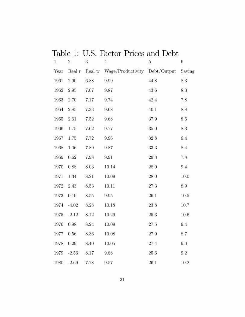
Table 1: U.S. Factor Prices and Debt1 2 3 4 5 6

Year Real r Real w Wage/Productivity Debt/Output Saving

1961 2.90 6.88 9.99 44.8 8.3

1962 2.95 7.07 9.87 43.6 8.3

1963 2.70 7.17 9.74 42.4 7.8

1964 2.85 7.33 9.68 40.1 8.8

1965 2.61 7.52 9.68 37.9 8.6

1966 1.75 7.62 9.77 35.0 8.3

1967 1.75 7.72 9.96 32.8 9.4

1968 1.06 7.89 9.87 33.3 8.4

1969 0.62 7.98 9.91 29.3 7.8

1970 0.88 8.03 10.14 28.0 9.4

1971 1.34 8.21 10.09 28.0 10.0

1972 2.43 8.53 10.11 27.3 8.9

1973 0.10 8.55 9.95 26.1 10.5

1974 -4.02 8.28 10.18 23.8 10.7

1975 -2.12 8.12 10.29 25.3 10.6

1976 0.98 8.24 10.09 27.5 9.4

1977 0.56 8.36 10.08 27.9 8.7

1978 0.29 8.40 10.05 27.4 9.0

1979 -2.56 8.17 9.88 25.6 9.2

1980 -2.69 7.78 9.57 26.1 10.2

31

Table 1 Continued: U.S. Factor Prices andDebt

1 2 3 4 5 6

Year Real r Real w Wage/Productivity Debt/Output Saving

1981 2.59 7.69 9.39 25.8 10.8

1982 6.03 7.68 9.22 28.6 10.9

1983 7.64 7.79 9.14 33.1 8.8

1984 7.69 7.80 8.88 34.0 10.6

1985 7.15 7.77 8.71 36.4 9.2

1986 6.24 7.81 8.61 39.5 8.2

1987 5.03 7.73 8.27 40.7 7.3

1988 4.88 7.69 8.08 40.9 7.8

1989 3.79 7.64 8.18 40.5 7.5

1990 3.33 7.52 8.06 42.0 7.8

1991 3.96 7.45 8.06 45.3 8.3

1992 4.52 7.41 7.88 48.2 8.7

1993 3.46 7.39 7.79 49.5 7.1

1994 4.81 7.40 7.61 49.4 6.1

1995 4.14 7.39 7.45 49.2 5.6

1996 3.80 7.43 7.43 48.5 4.8

1997 4.37 7.55 7.29 46.1 4.2

1998 4.09 7.75 7.29 42.9 4.7

1999 3.93 7.86 7.18 39.8 2.4

32