a neoclassical approach to the paradox of thriftalexmen/paradox_of_thrift.pdf · a neoclassical...
TRANSCRIPT

A Neoclassical Approach to the Paradox ofThrift∗
Preliminary and Incomplete
Alessandro MennuniUniversity of Southampton
September 26, 2013
Abstract
A test of the paradox of thrift is conducted throughout the lens of abusiness cycle model. To this aim, a simple extension of the neoclassicalframework with concave frontier is developed which leads to a dramaticimprovement on the prediction of the saving rate. Then, it is possible toisolate periods when saving changes are not a consequence of technologyshocks. A VAR identified through these episodes suggests that a 1%increase in the saving rate leads to half a percentage point decrease inoutput growth.
JEL Classification Codes: E13, E21, E32Keywords: Business cycle, technology shocks, saving shocks
∗I thank Martin Gervais, John Knowles and Paul Klein, Ramon Marimon, Dalibor Ste-vanovic for helpful comments. All remaining errors are mine.

1 Introduction
What is the effect of an increase in the saving rate? The paradox of thrift,
a famous conjecture popularaized by Keynes, but already debated at least
since the 18th century,1 is that an increase in the saving rate will depress
economic activity. In its strict form, the paradox states that the effect on out-
put is so strong to even reduce savings, thereby nullifying the original intent.
Throughout centuries, this conjecture received support within and beyond aca-
demic circles capturing media attention and affecting the policy debate, despite
the fact that there is virtually no empirical evidence in, or against its favor.
Chamley (2012), Huo and Rıos-Rull (2012) and Rendahl (2012) are examples
of the growing recent theoretical investigation spurred by the financial and
debt crisis.2 The main difficulty to empirically test the paradox of thrift hy-
pothesis is that savings are endogenous and strongly positively correlated to
economic activity. Unlike another popular conjecture of Keynes–the spending
multiplier–which engendered a multitude of empirical studies, the paradox of
thrift remained largely uninvestigated because it is hard to identify episodes
with exogenous changes in the saving rate.
This paper proposes a methodology to identify periods of times in which
saving rate changes were not due to the endogenous reaction to the business
cycle. To do so, the paper adopts a polar approach to the keynesian one; a
neoclassical business cycle model is used to develop a positive theory of savings
through which it is possible to isolate periods when changes in the saving rate
are not due to technological shocks. These periods are identified as those when
the saving rate moves in opposite directions to the one predicted by the model.3
1See Mandeville (1924) and Robertson (1892) among others.2A related but different literature studies the effects of financial shocks. Mian and Sufi
(2010) and Mian and Sufi (2012) provide empirical evidence that shocks to households bal-ance sheets affect consumption and employment. While financial shocks can lead to anincrease in the saving rate, the effects of an increase in the saving rate may not be confinedto the ones that follow from financial shocks. In fact, a saving rate increase may well improvefinancial conditions by increasing the supply of loanable funds, yet having negative aggregateeffects.
3It is important to notice that the correlation of output growth and the saving rate overthe selected sample is strongly positive. This suggests that the procedure does not onlyselect periods where savings and output move in opposite directions.
2

An S-VAR identified through these observations finds a negative effect of the
saving rate on output. Quantitatively, the VAR suggests that a 1% increase in
the saving rate leads to half a percentage point decrease in output growth.
To isolate saving rate changes not due to technology shocks, a simple real
business cycle model is simulated with the shocks and initial conditions iden-
tified from the data. Then, it is possible to compare true and simulated data
and identify the periods when the model prediction of the saving rate moves
in opposite direction to the data. This simulation procedure is not common
in the literature, where the identified shocks are only used to estimate their
stochastic processes. Then, simulations consist in drawing from these processes
and simulating around the balanced growth path. The alternative exercise pro-
posed here uncovers a puzzle that characterizes business cycle models driven
by technology shocks: they are very poor predictors of the saving rate time
series. This may prevent the ability of the model to filter periods of time when
changes in the saving rate are truly not consequential to technology shocks.4
A large part of the paper is devoted to address this issue by elaborating a
simple extension of the real business cycle model where the frontier between
consumption and investment goods can be concave.
Letting the frontier be concave relaxes the common assumption of linear
frontier maintained throughout the Dynamic Stochastic General Equilibrium
(DSGE) literature. Prominent examples include Greenwood et al. (2000), Cum-
mins and Violante (2002) and Fisher (2006). A concave frontier has important
implications for the equilibrium price between consumption and investment
goods, commonly used to identify I-shocks. This price equation is key because
without identifying investment shocks from the price equation, Justiniano et al.
(2008) find that the I-shock should be 4 times more volatile in order to match
business cycle fluctuations. This sharp contrast calls for an investigation of this
price equation (and consequently on the assumption of linear frontier) which,
despite its wide use, remained largely under-investigated. The paper points out
that the two shocks identified through a linear frontier are strongly negatively
4The paper distinguishes between neutral or total factor productivity shocks that hit allsectors of the economy (N-shock) and shocks specific to the productivity of investment goods(I-shock) (Greenwood et al. (1988)), which may be an important driver of the saving rate.
3

correlated. The paper argues that this fact is related to the poor fit of the
saving rate mentioned before, and points to a concave frontier. Indeed, with
a concave frontier, the model improves dramatically on the prediction of the
saving rate. The paper argues that this way the model improves the ability to
distinguish between the saving rate changes that are due to technology shocks
from those that are not.5
Methodologically, the approach proposed in this paper to identify saving
shocks is similar to the one adopted by the literature aimed at measuring
fiscal multipliers based on the narrative approach (Romer and Romer (2010)),
see Mertens and Ravn (2012) for a comprehensive analysis. There, external
information is used to identify fiscal shocks, here this kind of information,
which is not available, is replaced by a theory of savings. Then, it is possible to
isolate periods in which changes in the saving rate are not due to technological
shocks. Even during these periods, an assumption on the contemporaneous
effects between saving shocks and output is required to fully identify the VAR.
The paper shows that the negative effect of saving shocks on output holds true
for a wide range of identification assumptions.
The paper is organized as follows, the next section introduces a simple real
business cycle model and discusses the inability to match the saving rate. Sec-
tion 3 modifies the framework, introducing curvature in the transformation
frontier and illustrates the findings. Section 4 compares this model with cap-
ital adjustment costs. Section 5 tests the Paradox of Thrift hypothesis, and
Section 6 concludes. The Appendix contains data sources, the equilibrium
conditions and equivalent de-trended specifications.
5An alternative assumption to improve the prediction of the saving rate is to considercapital adjustment costs. The paper compares the effects of a concave frontier with thosethat come from adding capital adjustment costs. This friction only induces a negligibleimprovement on the saving rate prediction of the original model with linear frontier and donot affect the identification of the I-shock. Richer models of the business cycle also do notaffect the identification of I-shocks; for example Schmitt-Grohe and Uribe (2008), Justinianoet al. (2008) and Justiniano et al. (2009) consider medium-scale models with several frictionsthat do not affect the investment price equation.
4

2 A Real Business Cycle Model
Below follows a description of the standard growth model with investment-
specific technological change like, for instance, the one adopted in Fisher (2006).
The representative household solves the following problem, taking prices as
given:
max{ct,kt+1,nt}
E0
[∞∑t=0
βt
(log(ct)− χ
n1+1/νt
1 + 1/ν
)]s.t. ct + ptkt+1 = wtnt + ptkt(1 + rt − δ).
These preferences are adopted for instance by Rıos-Rull et al. (2009), as they
point out ν is the Frisch elasticity of hours, nt. χ scales the cost of working
and it determines the average level of hours. β is the discount factor. ct is
consumption, pt the price of capital in terms of consumption goods. wt is
the wage rate and rt the rental price of capital, kt. δ is the rate at which
capital depreciates. Production takes place through a constant returns to scale
Cobb-Douglas technology and capital evolves according to the law of motion
kt+1 − kt(1− δ) = VtAtkαt n
1−αt st,
while non-durable consumption is
ct = (1− st)Atkαt n1−αt (1)
where st is the fraction of physical production allocated to investment. Vt is
the investment shock, which only hits the production devoted to increasing the
capital stock. At is a neutral shock that hits both sectors in the same way.
These two shocks evolve according to the following processes:
Vt = γ0,vγt1,vV
ρvt−1e
εv,t , ρv ≤ 1, (2)
At = γ0,aγt1,aA
ρat−1e
εa,t , ρa ≤ 1. (3)
where εv,t and εa,t are independently and identically distributed random vari-
ables with standard deviation σεv and σεa . γ0,v, γ1,v, γ0,a, γ1,a are positive con-
stants.
5
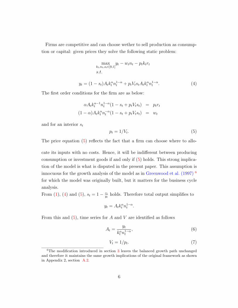
Firms are competitive and can choose wether to sell production as consump-
tion or capital: given prices they solve the following static problem:
maxkt,nt,st∈[0,1]
yt − wtnt − ptktrt
s.t.
yt = (1− st)Atkαt n1−αt + ptVtstAtk
αt n
1−αt . (4)
The first order conditions for the firm are as below:
αAtkα−1t n1−α
t (1− st + ptVtst) = ptrt
(1− α)Atkαt n−αt (1− st + ptVtst) = wt
and for an interior st
pt = 1/Vt. (5)
The price equation (5) reflects the fact that a firm can choose where to allo-
cate its inputs with no costs. Hence, it will be indifferent between producing
consumption or investment goods if and only if (5) holds. This strong implica-
tion of the model is what is disputed in the present paper. This assumption is
innocuous for the growth analysis of the model as in Greenwood et al. (1997) 6
for which the model was originally built, but it matters for the business cycle
analysis.
From (1), (4) and (5), st = 1− ctyt
holds. Therefore total output simplifies to
yt = Atkαt n
1−αt .
From this and (5), time series for A and V are identified as follows
At =yt
kαt n1−αt
, (6)
Vt = 1/pt. (7)
6The modification introduced in section 3 leaves the balanced growth path unchangedand therefore it maintains the same growth implications of the original framework as shownin Appendix 2, section A.2.
6

2.1 Correlation Between Shocks
The data are constructed by extending to 2012 II the data-set in Rıos-Rull
et al. (2009). In particular, data on the relative price of investment goods
extend those constructed by Gordon (1990), and successively by Cummins and
Violante (2002) and Fisher (2006). The dataset starts in 1948 I and the sources
are detailed in Appendix A.1. The two shocks are identified through equations
(6)–(7). To identify the neutral shock A, α is assumed equal to 0.36 and the
results of this section are robust to changes in this parameter.
ADF and Phillips-Perron tests accept the hypothesis of a unit root–stochastic
trend–for ln(A) and for ln(V ). I therefore estimate the regression
d ln(At) = 0.00230.0007
− 0.2920.086
d ln(Vt) + εt.
The relationship between these two variables is negative and strongly signifi-
cant. The correlation is strongly negative:
corr[d ln(A), d ln(V )] = −0.22.
Considering sub-samples of this sample gives similar results. I conclude that
the two time series for the shocks identified through the usual framework are
negatively correlated. This result is consistent with the finding of Schmitt-
Grohe and Uribe (2011) that the N-shock and the relative price of investment
are cointegrated.
2.2 Calibration
The other dimension where the misspecification is notable is that the model
predicts counter-factual savings rates. To asses this, the model is simulated
with the shocks identified from the data under a fairly standard parametrization
summarized in table 1.
The parameters of the model are β, α, δ, γ0,a, γ0,v, γ1,a, γ1,v, ρa, ρv, σεv , σεv , χ, ν.
In this model 1−α is equal to the labor share and hence α is calibrated equal
to 0.36.
ρa and ρv are restricted to be equal to one as suggested by the unit-root
tests. γ0,a, γ0,v, γ1,a, γ1,v, σεa , σεv are estimated by running OLS regressions on
7
the logs of the shocks. As is customary, it has implicitly been assumed that
there is zero covariance between the innovations.
δ is equal to 0.014, the average depreciation rate of total capital calculated
by Cummins and Violante (2002). The discount factor β is equal to 0.99. This
parametrization implies an average capital-output ratio of 10.2 an investment-
output ratio of 0.26 and an interest rate of 3.5%.
It remains to calibrate the parameters of the supply of labour: the critical
one is ν, which represents the Frisch elasticity. As pointed out by King and
Rebelo (1999) among others, how much of the business cycle can be explained
by technology shocks depends crucially on this parameter. Micro estimates
suggest a small number: a recent survey of the micro evidence by Chetty et al.
(2011) on the Frisch elasticity points to a value of 0.5 on the intensive margin
and of 0.25 on the extensive margin. Macro studies point to a larger role of
the extensive margin which theoretically can lead ν up to ∞ even when the
intensive margine is zero; see Rogerson (1988) and Hansen (1985). Prescott
(2004) considers a value of approximately 3. Rıos-Rull et al. (2009) estimate
the very model of this section using Bayesian techniques and find posterior
means between ν = 0.12 and ν = 1.56, depending on the variables and the
shocks included in the estimation.
In the context of the present application, which aims at measuring the extent
to which the model replicates some empirical observations, in particular the
observed saving rates, it seems instructive to consider a relatively high level of
Frisch elasticity, to give the model the best chance to match the data. Values
of 0.75, 1.5 and 3 are considered.
Finally, χ is chosen so that the average number of market hours is 0.33.
2.3 Saving Rate
To compare the saving rate of the model with the one in the data, the model is
simulated with the time series of innovations εa,t, εv,t identified from the data
and initial conditions for A0,V0 and k0, all coming from the data. To avoid
dependence on initial conditions, the model is compared to the data from 1960
III (the 50th period of simulation).
8
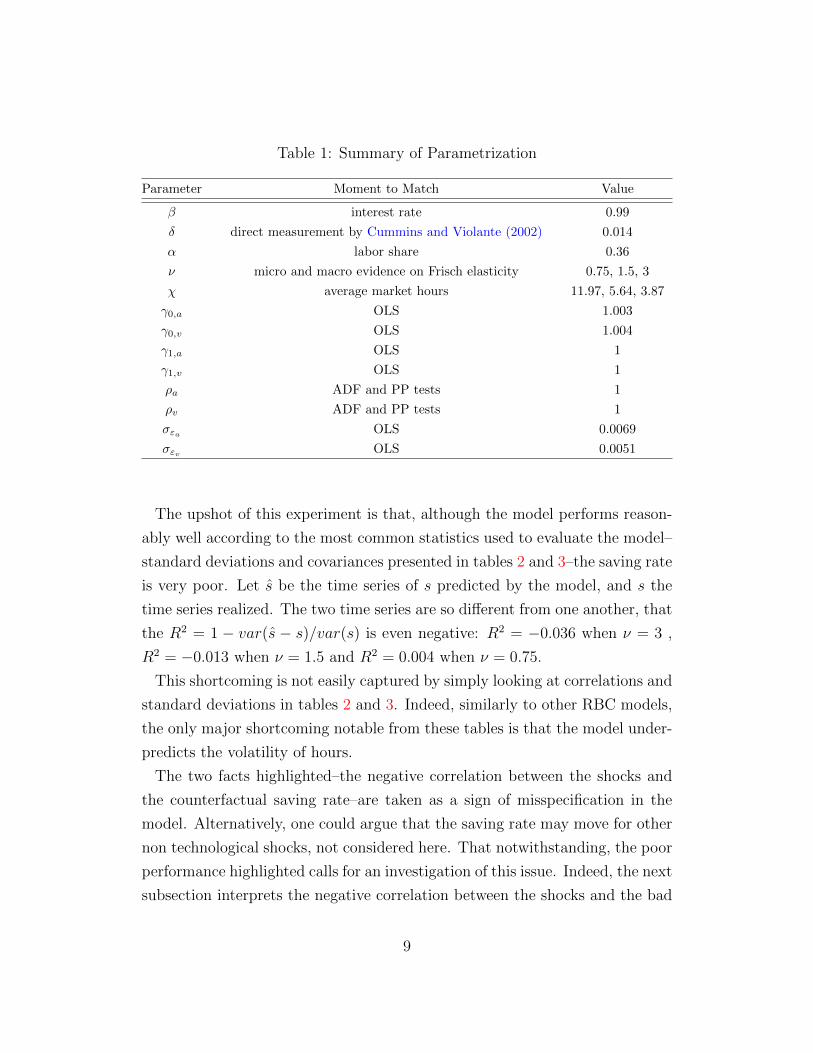
Table 1: Summary of Parametrization
Parameter Moment to Match Value
β interest rate 0.99
δ direct measurement by Cummins and Violante (2002) 0.014
α labor share 0.36
ν micro and macro evidence on Frisch elasticity 0.75, 1.5, 3
χ average market hours 11.97, 5.64, 3.87
γ0,a OLS 1.003
γ0,v OLS 1.004
γ1,a OLS 1
γ1,v OLS 1
ρa ADF and PP tests 1
ρv ADF and PP tests 1
σεa OLS 0.0069
σεv OLS 0.0051
The upshot of this experiment is that, although the model performs reason-
ably well according to the most common statistics used to evaluate the model–
standard deviations and covariances presented in tables 2 and 3–the saving rate
is very poor. Let s be the time series of s predicted by the model, and s the
time series realized. The two time series are so different from one another, that
the R2 = 1 − var(s − s)/var(s) is even negative: R2 = −0.036 when ν = 3 ,
R2 = −0.013 when ν = 1.5 and R2 = 0.004 when ν = 0.75.
This shortcoming is not easily captured by simply looking at correlations and
standard deviations in tables 2 and 3. Indeed, similarly to other RBC models,
the only major shortcoming notable from these tables is that the model under-
predicts the volatility of hours.
The two facts highlighted–the negative correlation between the shocks and
the counterfactual saving rate–are taken as a sign of misspecification in the
model. Alternatively, one could argue that the saving rate may move for other
non technological shocks, not considered here. That notwithstanding, the poor
performance highlighted calls for an investigation of this issue. Indeed, the next
subsection interprets the negative correlation between the shocks and the bad
9

Table 2: Standard deviations
Output Consumption Investment Hours
Data 1.57 0.67 5.21 1.88
Model
ν = 3 1.03 0.72 2.73 0.47
ν = 1.5 0.97 0.72 2.47 0.34
ν = 0.75 0.92 0.72 2.25 0.22
Table 3: Correlation with output
Output Consumption Investment Hours
Data 1 0.40 0.95 0.87
Model
ν = 3 1 0.76 0.88 0.74
ν = 1.5 1 0.78 0.86 0.69
ν = 0.75 1 0.80 0.84 0.64
fit in the saving rate as being suggestive of a concave transformation frontier.
2.4 The Case for Curvature in the Transformation Fron-
tier
Since the model can be expressed in recursive form with state variablesAt, Vt, kt,
assume that the true price equation is of the form
pt = p(At, Vt, kt) (8)
and let the total production measured in consumption units be
yt = y(At, Vt, kt). (9)
Considering instead the price equation (5) and the aggregate resource con-
straint (4) would wrongly impute all the increase (decrease) in the relative
price to a decrease (increase) in Vt, and all the variation in production not
10

explained by kt to At. If instead ∂p∂At
> 0, increases in pt may be due to in-
creases in At, and when this happens, also yt increases through At. With the
misspecified policy functions, the increase in the price would be attributed to
a decrease in Vt, while instead only an increase in At occurred. This leads
to the negative correlation between At and Vt, which is not a pure negative
correlation between the two shocks, but is due to the misspecification of the
model.
The misspecification also leads to counter-factual saving rates: when there is
an increase in At, according to the true policy function (8) pt grows. When this
happens, the original model identifies a decrease in Vt. Because the productivity
of investments decreased, the saving rate predicted by the model decreases. If,
on the contrary, no I-shock occurred, the increase in At would imply an increase
in the saving rate. Therefore, a misspecified price equation leads to counter-
factual saving rates.
It follows from these considerations that a model used to measure these
shocks for the business cycle should be specified in a way such that the time
series for the shocks that it predicts, appear to be independent and match as
closely as possible the saving rate time series. These are the two facts that will
be targeted in the specification and calibration of the model presented in the
next section.
3 The Modified Framework
Consider the following modification to the model: a generic firm produces
yt = Atkat n
1−at (1− st)1−ρ + ptVtAtk
at n
1−at s1−ρt , (10)
where ρ ∈ [0, 1). st measures the share of inputs allocated to the production
of investment goods.
Therefore,
ct = Atkat n
1−at (1− st)1−ρ (11)
kt+1 − kt(1− δ) = VtAtkat n
1−at s1−ρt . (12)
11

The firm can produce for both sectors and solves the following problem:
maxk,n,s∈[0,1]
Atkat n
1−at (1− st)1−ρ + ptVtAtk
at n
1−at s1−ρt − wn− rpk. (13)
When ρ > 0, the marginal productivity of consumption and of investment
goods is decreasing and therefore the firm will always choose to produce both
types of goods even when pV differs from one. This very simple specification,
capturing curvature in somewhat reduced form, has the advantage of being
closely related to the original framework from which it departs, thereby being
able to isolate the role of curvature from any other possible change that can
be made. In particular, this technology preserves the assumption of constant
returns to scale, so the problem remains consistent with perfect competition
where the size and number of firms does not matter and firms take prices as
given.
The equilibrium conditions that correspond to a competitive equilibrium are
reported in appendix A.2 and are essentially unchanged with respect to the
usual framework, except for the resource constraints above and for the price
equation, which comes from the optimal choice of st:
ptVt =(1− st)−ρ
s−ρt. (14)
This price equation shows that the change in the relative price is not only due
to a change in Vt, but it also depends on the change in st, i.e. on the change
in the relative demand for the two goods. This in turns depends on both the
shocks and on capital. The reason for this is that the production possibility
frontier is concave as illustrated in Figure 1.
12

Figure 1: Production possibility frontier
When ρ = 0 the price equation (and the whole model) boils down to the
usual framework. The next section pins down ρ.
3.1 Estimating ρ
As mentioned, two strategies are employed. The first is to pick ρ such that the
shocks identified are uncorrelated. Similarly to the original model, the shocks
can be identified from the production equation(10) and the price equation (14)
as
V =
(1− ss
)−ρ1
p(15)
A =y
kαt n1−αt [(1− s)1−ρ + pV s1−ρ]
. (16)
As becomes clear from observing the two equations above, to identify the
shocks, it is first necessary to identify s. From the resource constraints (11)
and (12) it follows that(1− s)1−ρ
pV s1−ρ=
c
y − c, (17)
Substituting into equation (14) one gets
s = 1− c
y. (18)
s is the saving rate which can be taken from the data.
With s, k, y, p and n at hand, at each ρ correspond time series for A and V
through (15) and (16) and a correlation corr(εa, εv) from the estimation of the
processes (2) and (3). Figure 2 shows this correlation as a function of ρ.
13

Figure 2: Correlation between the shocks’innovations as a function of ρ.
As it can be observed, the correlation is concave, and it crosses zero twice.
It should be clear that starting with a linear frontier (ρ = 0), an increase
in ρ reduces the correlation for the arguments in section 3. The picture also
shows that for ρ sufficiently high, the correlation is decreasing in ρ. This can
be rationalized as follows: after a positive I-shock, inter-temporal optimiza-
tion calls for an increase in the saving rate s. The increase in s implies that
the marginal productivity of consumption goods (1 − ρ)Atkαt n
1−αt (1 − st)
−ρ
increases. The marginal productivity of investments, measured in consump-
tion goods ptVt(1− ρ)Atkαt n
1−αt s−ρt also has to increase, since the two marginal
productivities must be equal in equilibrium. This calls for an increase in pV .
Compared with the original framework, the price reacts less to a change in the
investment shock, making the product pV procycliclal. Unlike what happens
in the original framework, the fact that pV increases even after an investment
shock, makes aggregate productivity increase. With too much curvature, this
effect may be exacerbated, total output is predicted to increase more than in
the data and a negative N-shock is identified. Thus, the correlation between
the two shocks is negative if ρ is too high.
14

The second strategy to pin down ρ is to maximize the R2 of the saving rate
predicted by the model given the shocks identified.7 This is done through a
grid search over ρ and for each value of ρ, by doing the following: 1. given the
other parameters, back out the two shocks time series through (15) and (16);
2. Estimate the parameters of the shocks’ processes. 3. Solve the model.8 4.
Simulate given the shocks identified, and compute the R2 after discarding the
first 50 observations.
Figure 3 plots the R2 as a function of ρ.
Figure 3: R2 as a function of ρ.
There is a kink when ρ is approximately 0.06. At that point the N-shock
becomes stationary, this leads to a much higher portion of variance explained.
With Frisch elasticity ν = 1.5, the value of ρ that gives the highest R2 is
ρ = 0.243. R2 of 0.476 is a substantial increase in the portion of variance of
the saving rate explained by this model compared to the original framework
where the variance explained is essentially zero. With ν = 0.75 this procedure
leads to ρ = .233 with R2 = .470. With ν = 3, ρ = .252 and R2 = .481.
7This is equivalent to minimize the squared sum of residuals s− s.8As explained below, with higher values of ρ the N-shock is stationary. When this is the
case, the model is solved assuming a stationary process for the N-shock and maintaining anon-stationary process for the I-shock.
15

Strikingly, these estimates for ρ are very close to the highest value obtained
with the other procedure. In fact the properties of the shock processes are
essentially unchanged when ρ is found by maximizing the saving rate or with
the highest value obtained through the correlation procedure. This suggests
that among the two values estimated through the correlation procedure, the
highest value may be favored. To clear out any doubt, a GMM procedure is ran
where the moments above–the correlation between the residuals corr(εa, εv) and
the sum of squares (s− s)–are combined. Not surprisingly, this procedure gives
a value between the one that maximizes the R2 and the highest value obtained
through the correlation procedure. These estimations are summarized in table
3.1. The table also reports the standard deviation of the parameter estimated
and the p-value of the J test for over-identification, which does not reject the
null that the model is correctly specified. Given the asymptotic normality of
the GMM estimator, standard errors suggest that ρ is significantly larger than
zero.
Table 4: Curvature Parameter ρ
Method Estimate St.Dev J test (p-value)
1st strategy 0.279 - -
ν = 0.75
2nd strategy 0.233 - -
GMM 0.266 0.065 0.424
ν = 1.5
2nd strategy 0.243 - -
GMM 0.265 0.047 0.428
ν = 3
2nd strategy 0.252 - -
GMM 0.267 0.049 0.432
Results are not very sensitive to the stand taken on ν. Thus, ν = 1.5 is
considered hereafter unless otherwise specified.
Figure 4 compares the saving rate from the data to those of the model with
ρ = 0.265 and ρ = 0. As is evident, curvature induces a substantial improve-
16
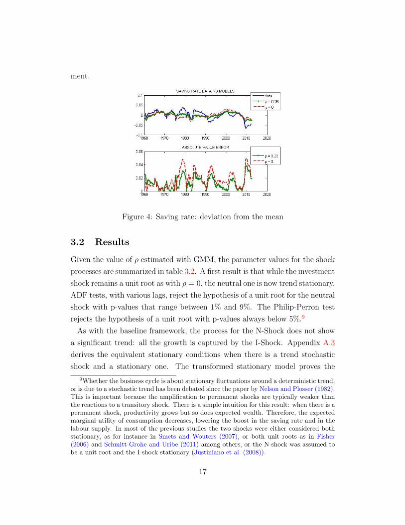
ment.
Figure 4: Saving rate: deviation from the mean
3.2 Results
Given the value of ρ estimated with GMM, the parameter values for the shock
processes are summarized in table 3.2. A first result is that while the investment
shock remains a unit root as with ρ = 0, the neutral one is now trend stationary.
ADF tests, with various lags, reject the hypothesis of a unit root for the neutral
shock with p-values that range between 1% and 9%. The Philip-Perron test
rejects the hypothesis of a unit root with p-values always below 5%.9
As with the baseline framework, the process for the N-Shock does not show
a significant trend: all the growth is captured by the I-Shock. Appendix A.3
derives the equivalent stationary conditions when there is a trend stochastic
shock and a stationary one. The transformed stationary model proves the
9Whether the business cycle is about stationary fluctuations around a deterministic trend,or is due to a stochastic trend has been debated since the paper by Nelson and Plosser (1982).This is important because the amplification to permanent shocks are typically weaker thanthe reactions to a transitory shock. There is a simple intuition for this result: when there is apermanent shock, productivity grows but so does expected wealth. Therefore, the expectedmarginal utility of consumption decreases, lowering the boost in the saving rate and in thelabour supply. In most of the previous studies the two shocks were either considered bothstationary, as for instance in Smets and Wouters (2007), or both unit roots as in Fisher(2006) and Schmitt-Grohe and Uribe (2011) among others, or the N-shock was assumed tobe a unit root and the I-shock stationary (Justiniano et al. (2008)).
17

existence of a Balanced Growth Path and allows for a recursive formulation.
From this it becomes clear that the model has the same long-run implications
as the original framework: the expected growth rates of all the variables are
unchanged.
Table 5: Other Parameter Values
γ0,a γ1,a ρa σεa γ0,v γ1,v ρv σεv
1.017 1.000 0.983 0.006 1.000 1.005 1.000 0.012
Tables 6 and 7 report standard deviations and correlations with output.
Table 6: Standard deviations (ν = 1.5)
Output Consumption Investment Hours
Data 1.57 0.67 5.21 1.88
Model
ρ = 0 0.97 0.72 2.47 0.34
ρ = 0.265 0.92 0.64 2.54 0.36
Table 7: Correlation with output (ν = 1.5)
Output Consumption Investment Hours
Data 1 0.40 0.95 0.87
Model
ρ = 0 1 0.78 0.86 0.69
ρ = 0.265 1 0.75 0.87 0.74
It is possible to revisit the age old question originated by Kydland and
Prescott (1982), of how much of the business cycle is accounted for by technol-
ogy shocks. With curvature, technology shocks account for 59% of the aggre-
gate fluctuations in output, slightly less than with a linear frontier. However,
the volatility of hours and their correlation with output are slightly higher.
18
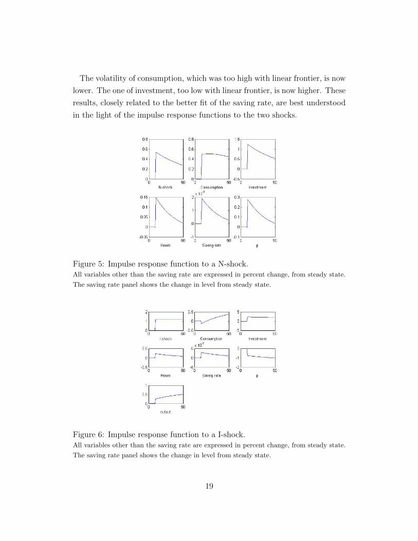
The volatility of consumption, which was too high with linear frontier, is now
lower. The one of investment, too low with linear frontier, is now higher. These
results, closely related to the better fit of the saving rate, are best understood
in the light of the impulse response functions to the two shocks.
Figure 5: Impulse response function to a N-shock.All variables other than the saving rate are expressed in percent change, from steady state.
The saving rate panel shows the change in level from steady state.
Figure 6: Impulse response function to a I-shock.All variables other than the saving rate are expressed in percent change, from steady state.
The saving rate panel shows the change in level from steady state.
19

1. As shown in Figure 5, after a positive neutral shock, households want to
increase the investment rate in order to smooth consumption. With a
concave frontier, firms are reluctant to accommodate this excess demand
of investment goods and the price has to increase to induce them to adjust
supply.
This highlights the fact that the change in the relative price of goods is
not all due to the I-shock and how it could be misleading to identify the
investment shock in the usual way.
The fact that p increases after an N-shock implies that consumption
responds more to the shock relative to the linear framework; the increase
in the relative price induces agents to increase consumption, preventing
the saving rate to increase as mach as in the linear framework, where the
investment price does not depend on the N-shock. This is a feature typical
of two-goods models with imperfect input reallocation, which turned out
to imply a high equity premium as has been shown by Boldrin et al.
(2001).
2. As shown in Figure 6, after an I-shock consumption decreases. However,
the decrease is demeaned by the smaller (compared to the linear frame-
work) decrease in the price that follows the investment shock. Thus pV
increases, contributing to the increase in GDP measured in consumption
goods. Given this increase in GDP, it is possible to increase the saving
rate without an abrupt decrease in consumption.
The extent to which this dynamics is an improvement relative to the linear
framework can be appreciated by comparing it with the impulse responses from
the linear framework, once the negative correlation is taken into account. To
this aim, a Choleski decomposition is applied to the covariance matrix between
the innovations, so that an innovation to the I-shock can affect the N-shock.
As shown in Figure 7, after a positive I-shock output decreases for a prolonged
period of time. This is because the I-shock also leads to a negative effect on the
N-shock. Furthermore, if the negative effect on the N-shock is large enough,
an I-shock also induces a decrease in the saving rate and hours as shown in
20

Figure 8. These figures highlight how the typical propagation of I-shocks in the
model with linear frontier is hard to rationalize and calls for a concave frontier.
One reason why these effects have been overseen might be that typically the
correlation between the shocks is ignored. One exception is Schmitt-Grohe and
Uribe (2011) who assume a co-integrated process for the two shocks.
Figure 7: Impulse response function to a I-shock with ρ = 0.All variables other than the saving rate are expressed in percent change, from steady state.
The saving rate panel shows the change in level from steady state.
Figure 8: Impulse response function to a I-shock with ρ = 0 and strong negativeeffect on N-shock.All variables other than the saving rate are expressed in percent change, from steady state.
The saving rate panel shows the change in level from steady state.
21

Finally, it is possible to get a sense of the relative importance of the two
shocks. Running the model with either only N-shocks or I-shocks, it is found
that most of the variability of output comes from the N-shock, while most of
the one of hours comes from the I-shock. In particular, running the model with
N-shocks only, 66% of the standard deviation of output is explained but only
6% of the one of hours.10 Running the model only with I-shocks only, 20%
of the standard deviation of output is explained and 18% of the one of hours.
The fact that hours are more sensitive to the I-shock has also been found by
Rıos-Rull et al. (2009).
4 Capital Adjustment Costs
This section assesses the extent to which capital adjustment costs can be an
alternative way to improve on the dimensions considered in this paper.
The household is faced with the following capital accumulation equation:
kt+1 = kt(1− δ) + ψ
(itkt
)kt (19)
where it = VtAtkαt n
1−αt st is investment goods and ψ(·) is an increasing and
concave function. Following Jermann (1998) the adjustment cost function is
ψ
(itkt
)=
a1
1− ζ
(itkt
)1−ζ
+ a2, ζ > 0. (20)
The budget constraint is
ct + pk,tit = wtnt + ktRt. (21)
The equilibrium conditions are reported in Appendix A.2. The first finding
is that since the firm problem is unchanged, the relative price equation that
identifies I-shocks is not affected by capital adjustment costs.11 Therefore,
capital adjustment costs do not help making the shocks orthogonal to each
other.10In the linear case N-shocks account for 56% of the standard deviation of output and 7%
of the one of hours. Curvature amplifies the effects of N-shocks.11Assuming that adjustment costs are borne by the firms would be equivalent.
22

Following Jermann (1998), ζ = 0.23. It determines the elasticity of invest-
ments to Tobin Q. a1 and a2 are such that the model has the same deterministic
steady state as in the case with no adjustment costs.
Simulating the model with the shocks identified, gives an R2 of 0.048. This
is a modest improvement relative to the linear case with no adjustment costs,
and it is clearly worse than with a concave transformation frontier.
Tables 8 and 9 compare the business cycle statistics of the model with adjust-
ment costs, to the one with a concave transformation frontier. Adjustment costs
dump the volatility of investments, which was already too low, and increase
the one of consumption beyond the one in the data. This is intuitive given that
with adjustment costs, capital has to be kept smooth, so consumption has to
adjust.12 This is also reflected in a too high correlation of consumption with
output. The standard deviation of output is also slightly lower while the one
of hours is less than half the one with a concave frontier.
From these findings, it seems clear that adjustment costs do not provide a
substitute to a concave frontier for the dimensions this paper is concerned with.
Table 8: Standard deviations (ν = 1.5)
Output Consumption Investment Hours
Data 1.57 0.67 5.21 1.88
Models
Adjustment costs 0.90 0.77 1.48 0.16
ρ = 0.265 0.92 0.64 2.54 0.36
12This is because this friction introduces inter-temporal adjustment costs. Instead, concav-ity in the transformation frontier is a concept that is closer to the intra-temporal adjustmentcosts between capital goods considered by Huffman and Wynne (1999).
23

Table 9: Correlation with output (ν = 1.5)
Output Consumption Investment Hours
Data 1 0.40 0.95 0.87
Models
Adjustment costs 1 0.96 0.91 0.60
ρ = 0.265 1 0.75 0.87 0.74
5 The Paradox of Thrift
With a sensible theory of how savings react to technological shocks, it is possible
to identify periods in which savings have not responded to technological shocks
and asses the implication of these movements in savings on the business cycle.
These periods are taken to be those when the true data series moves in opposite
direction to the one predicted by the model given the identified technology
shocks.13 On this sub-sample, I estimate a VAR of order one with the saving
rate and output growth.14
To identify the impulse responses, I assume a Choleski decomposition, where
saving rates can affect output growth on impact but output growth can affect
savings only with a lag. The extent to which this assumption is extreme is
lessened by the fact that the sample excludes periods when the saving rate
reacts to technology shocks.
The mentioned sampling procedure selects 20 observations out of the 210 con-
sidered (1960.III-2012.II).15 Thus, the probability that the saving rate moves
in the opposite direction than the one predicted by the model is 9.5%. Of these
20 observations, 5 occur while output growth is below average and 15 while
13Alternatively, one could use the model to fully identify saving shocks as residuals. Theprocedure adopted here is preferred because it minimizes the extent to which it relies on thetheoretical model.
14The choice of only one lag is dictated by the small sample size. However, even onthe entire sample, Schwartz’s Bayesian information criterion, and the Hannan and Quinninformation criterion suggest to use one lag, the Akaike’s information criterion suggests twolags. Estimating a VAR 2 does not change the direction of the impulse responses.
15The first observations of the sample are excluded to avoid that the simulations dependon initial conditions. Including these observations in the VAR does essentially not affect theresults.
24
output growth is above average. Thus the procedure does not over-sample re-
cessions. It is also worth noticing that the correlation between the saving rate
and output growth over the selected sub-sample is 0.39. It is actually higher
than the one on the entire sample: 0.28. Therefore, the procedure does not
simply select periods where the two variables move in opposite directions. The
periods selected are reported in Table 10.16
Table 10: Selected Sample
60.IV 64.I 64.III 66.I 70.III 70.IV 77.I 79.IV 84.IV 85.IV
86.II 90.II 91.III 92.II 92.IV 98.III 01.III 02.I 03.I 09.IV
Figure 9 left panels show the impulse responses to a one standard deviation
innovation in savings. An increase in the saving rate induces a contraction
in output growth. The VAR estimated over this sample has very small inno-
vations, with a standard deviation of 0.22% (i.e. a one standard deviations
shock induces the saving rate to go from 15 to 15.22%). To get a sense of
the magnitude, it is instructive to consider a 1% increase in the saving rate.
Such shock would induce a 0.56% decline in output growth (for instance, if the
saving rate goes from 15 to 16%, output drops from 2 to 1.44%). The negative
effect lasts for 3 quarters. Thereafter, there is a mild but very long positive
effect on output growth.17
16Starting from the beginning of the sample, five more periods would be selected: 51.IV,53.II, 57.I, 57.IV, 58.II.
17It is also possible to estimate the VAR on the entire sample, and only use the sub-samplefor the identification of the impulse responses. This procedure does not qualitatively affectthe results.
25

Figure 9: Impulse response function of an S-VAR.
The Figure also shows the response to an output shock (other than techno-
logical). Savings react positively from one period after the shock. Presumably,
the impact effect on savings may be positive too, contrarily to the decomposi-
tion assumption. To check for robustness, I achieve identification by assuming
alternative responses of savings to an output shock.
5.1 Alternative Residual Decompositions
Calling η the residuals from the VAR, the structural shocks ε can be identified
via a matrix M :
η = Mε. (22)
Normalizing the shocks ε to have unitary variance, the matrix M has to be
such that
MM ′ = Σ, (23)
where Σ is the covariance matrix of η. Because Σ is symmetric, equation (23)
pins down three out of the four parameters in M . The Choleski decomposi-
tion puts M1,2 = 0. Figure 10 shows M2,1, the impact response of income to
a unitary saving shock, for all possible alternative assumptions for M1,2. The
range for M1,2 is [−0.002, 0.002] because outside this range, M is imaginary.
26

As the figure shows, the impact response of output to a saving shock is nega-
tive for M1,2 > −0.0005. And for positive, more plausible values of M1,2 the
effect on income is negative and even stronger than the one of the Choleski
decomposition.
Figure 10: Impact response of income to a saving shock for alternative identi-
fication assumptions.
I conclude that this analysis confirms the conjecture that a savings shock
depresses economic activity in the short run. Notice that the sample selection
procedure is important for this result: the impulse response of output to a
saving shock is positive when a Choleski decomposition is used to decompose
residuals over the entire sample.
6 Conclusions
To test the paradox of Thrift, a neoclassical business cycle model is used to
identify periods when saving rate changes are not consequential to technology
shocks.
A by-product of this methodology is to show that the basic framework
adopted by the DSGE literature predicts counter-factual saving rates and neg-
atively correlated neutral and investment shocks. I argue that this counter-
27

factual observation emanates from the assumed linearity of the transformation
frontier between consumption and investment goods.
A simple extension of the original framework is developed that allows for
the transformation frontier to be concave. With a concave frontier, the model
improves dramatically on the prediction of the saving rate, dimension that
cannot be significatively improved with alternative mechanisms such as capital
adjustment costs.
Given the promising results and the simple modeling approach, introducing
curvature in the transformation frontier into the large-scale models adopted by
the DSGE literature may be a fruitful avenue to pursue. Another interesting
direction for future research is to investigate the underlying factors that lead
to an aggregate concave frontier.
With a theory of savings that fits the data, it is possible to isolate periods
in which changes in the saving rate are not due to technological shocks and
test the paradox of thrift hypothesis: that a positive saving shock contracts
economic activity. A VAR estimated through this sample suggests that a 1%
increase in the saving rate (for instance, from 15 to 16%) leads to a 0.56%
decrease in output growth. After a few periods, the effect on output growth
is positive. Given these findings, research should be devoted to study the
mechanism through which an increase in savings depresses economic activity.
References
Boldrin, M., L. Christiano, and J. Fisher (2001). Habit persistence, assets
returns and the business cycle. American Economic Review 91.
Chamley, C. (2012). A paradox of thrift in general equilibrium without forward
markets. Journal of the European Economic Association (10), 12151235.
Chetty, R., A. Guren, D. S. Manoli, and A. Weber (2011, January). Does
indivisible labor explain the difference between micro and macro elastici-
ties? a meta-analysis of extensive margin elasticities. Working Paper 16729,
National Bureau of Economic Research.
28

Cummins, J. and G. Violante (2002, April). Investment-specific technical
change in the u.s. (1947-2000): Measurement and macroeconomic conse-
quences. Review of Economic Dynamics 5(2).
Fisher, J. (2006, June). The dynamic effects of neutral and investment-specific
technology shocks. Journal of Political Economy 114(3).
Gordon, R. (1990). The measurement of durable goods prices. University of
Chicago Press .
Greenwood, J., Z. Hercowitz, and G.Huffman (1988, June). Investment, ca-
pacity utilization and the business cycle. American Economic Review 78.
Greenwood, J., Z. Hercowitz, and P. Krusell (1997). Long-run implications of
investment-specific technological change. American Economic Review 87(3).
Greenwood, J., Z. Hercowitz, and P. Krusell (2000). The role of invest-ment
speci.c technological change in the business cycle. European Economic Re-
view .
Hansen, G. D. (1985). Indivisible labor and the business cycle. Journal of
Monetary Economics 16 (3), 309 – 327.
Huffman, G. and M. Wynne (1999). The role of intratemporal adjustment
costs in a multisector economy. Journal of Monetary Economics 43(2).
Huo, Z. and J.-V. Rıos-Rull (2012, December). Engineering a paradox of thrift
recession. Quarterly Review .
Jermann, U. J. (1998, April). Asset pricing in production economies. Journal
of Monetary Economics 41 (2), 257–275.
Justiniano, A., G. Primiceri, and A. Tambalotti (2008). Investment shocks and
business cycles. Federal Reserve Bank of New York Staff Reports 322.
Justiniano, A., G. Primiceri, and A. Tambalotti (2009). Investment shocks and
the relative price of investment. CEPR 7597.
29

King, R. G. and S. T. Rebelo (1999, June). Resuscitating real business cycles.
In J. B. Taylor and M. Woodford (Eds.), Handbook of Macroeconomics, Vol-
ume 1 of Handbook of Macroeconomics, Chapter 14, pp. 927–1007. Elsevier.
Kydland, F. E. and E. C. Prescott (1982). Time to build and aggregate fluc-
tuations. Econometrica 50 (6), pp. 1345–1370.
Mandeville, B. (1732 / 1924). The fable of the bees: or. private vices, public
benefits. London: Oxford University Press.
Mertens, K. and M. Ravn (2012). A reconciliation of svar and narrative esti-
mates of tax multipliers. CEPR Discussion Paper 8973, Centre for Economic
Policy Research.
Mian, A. and A. Sufi (2010, May). The great recession: Lessons from microe-
conomic data. American Economic Review 100 (2), 51–56.
Mian, A. R. and A. Sufi (2012, February). What explains high unemployment?
the aggregate demand channel. NBER Working Papers 17830, National
Bureau of Economic Research, Inc.
Nelson, R. and C. Plosser (1982). Trends and random walks in macroeconomic
time series. Journal of Monetary Economics .
Prescott, E. C. (2004). Why do americans work so much more than europeans?
Quarterly Review (Jul), 2–13.
Rendahl, P. (2012, February). Fiscal policy in an unemployment crisis. Cam-
bridge Working Papers in Economics 1211, Faculty of Economics, University
of Cambridge.
Robertson, J. M. (1892). The Fallacy of Saving. New York.
Rogerson, R. (1988). Indivisible labor, lotteries and equilibrium. Journal of
Monetary Economics 21 (1), 3 – 16.
30

Romer, C. D. and D. H. Romer (2010). The macroeconomic effects of tax
changes: Estimates based on a new measure of fiscal shocks. American
Economic Review 100 (3), 763–801.
Rıos-Rull, J.-V., F. Schorfheide, C. Fuentes-Albero, M. Kryshko, and R. San-
taeulalia-Llopis (2009, September). Methods versus substance: Measuring
the effects of technology shocks on hours. Working Paper 15375, National
Bureau of Economic Research.
Schmitt-Grohe, S. and M. Uribe (2008). What’s news in business cycles. Na-
tional Bureau of Economic Research NBER Working Papers 14215.
Schmitt-Grohe, S. and M. Uribe (2011, January). Business cycles with a com-
mon trend in neutral and investment-specific productivity. Review of Eco-
nomic Dynamics 14 (1), 122–135.
Smets, F. and R. Wouters (2007, June). Shocks and frictions in U.S. business
cycles: A Bayesian DSGE approach. American Economic Review 97 (3),
586–606.
A Appendix
A.1 Data
The data set extends to 2012 II, the data set of Rıos-Rull et al. (2009), see
their online appendix for the construction of a price index for consumption, a
quality-adjusted price index for investment, quality-adjusted investment and
capital.
A.1.1 Raw Data Series
Bureau of Labor Statistics (BLS)
Hours, ID PRS85006033
Civilian Noninstitutional Population, ID LNU00000000
31

National Income and Product Accounts (NIPA-BEA)
Nominal Gross National Product, Table 1.7.5
Price Indexes for Private Fixed Investment by Type, Table 5.3.4
Private Fixed Investment by Type, Table 5.3.5
Gross Domestic Product, Table 1.1.5
Government Consumption Expenditures and Gross Investment, Table 3.9.5
Personal Consumption Expenditures by Major Type of Product, Tables 2.3.5
(Nominal) and 2.3.3 (Quantity Index)
Cummins and Violante (2002)
Annual Quality-Adjusted Price Index for Investment in Equipment
Annual Quality-Adjusted Depreciation Rates for Total Capital
A.2 Balanced Growth Path with trend-stochastic shocks
The equilibrium conditions are
λt = βEt
{1
ct+1
Rt+1 + λt+1
(1− δ + ψ
(it+1
kt+1
)− ψ′
(it+1
kt+1
)it+1
kt+1
))(24)
1
ctpt = λtψ
′(itkt
)(25)
wtct
= ξn1/νt (26)
kt+1 = (1− δ)kt + ψ
(itkt
)kt (27)
ptVt =(1− st)−ρ
s−ρt(28)
it = VtAtkαt n
1−αt s1−ρt (29)
ct = Atkαt n
1−αt (1− st)1−ρ (30)
wt = (1− α)Atkαt n−αt
[(1− st)1−ρ + ptVts
1−ρt
](31)
32
Rt = αAtkα−1t n1−α
t
[(1− st)1−ρ + ptVts
1−ρt
]. (32)
The budget constraint
ct + ptit = wtnt + ktRt (33)
is implied by Walras’ law.
Let zt = A1
1−αt V
α1−αt . Consider the auxiliary variables ct = ct
zt−1, kt = kt
zt−1Vt−1,
pt = ptVt−1, it = itzt−1Vt−1
, λt = λtzt−1Vt−1, wt = wtzt−1
, Rt = RtVt−1. Substituting
these expressions into equations (24)–(32), one obtains the following equations,
which are stationary in the auxiliary variables:18
λt = βEt
{zt−1Vt−1ztVt
(Rt+1
ct+1
+ λt+1
(1− δ + ψ
(it+1
kt+1
)− ψ′
(it+1
kt+1
)it+1
kt+1
))}(34)
1
ctpt = λtψ
′(it
kt
)(35)
wtct
= ξn1/νt (36)
kt+1ztVt
zt−1Vt−1= (1− δ)kt + ψ
(it
kt
)kt (37)
ptVtVt−1
=(1− st)−ρ
s−ρt(38)
it(zt−1Vt−1)
1−α
AtVt= kαt n
1−αt s1−ρt (39)
ctz1−αt−1 V
−αt−1
At= kαt n
1−αt (1− st)1−ρ (40)
wtz1−αt−1 V
−αt−1
At= (1− α)kαt n
−αt
[(1− st)1−ρ + pt
VtVt−1
s1−ρt
](41)
Rt(zt−1Vt−1)
1−α
AtVt−1= αkα−1t n1−α
t
[(1− st)1−ρ + pt
VtVt−1
s1−ρt
]. (42)
18Since the auxiliary variables are independent of ρ, it follows that the trends in the originalvariables are not affected by ρ.
33

These equations imply that the stationary budget constraint is
ct + ptit = wtnt + ktRt. (43)
When the productivity processes are trend stochastic (ρa and ρv equal to
one), the productivity processes (2) and (3) reduce to
At = γaAt−1eεa,t (44)
and
Vt = γvVt−1eεv,t . (45)
This is because the growth factors AtAt−1
and VtVt−1
are stationary and thus the
trend factors γ1,a and γ1,v are equal to one. Then, equations (34)–(42) further
simplify to
λt = βEt
{(γaγve
εa,t+εv,t) 1α−1
(Rt+1
ct+1
+ λt+1
(1− δ + ψ
(it+1
kt+1
)− ψ′
(it+1
kt+1
)it+1
kt+1
))}(46)
1
ctpt = λtψ
′(it
kt
)(47)
wtct
= ξn1/νt (48)
kt+1
(γaγve
εa,t+εv,t) 1
1−α = (1− δ)kt + ψ
(it
kt
)kt (49)
ptγveεv,t =
(1− st)−ρ
s−ρt(50)
it =(γaγve
εa,t+εv,t)kαt n
1−αt s1−ρt (51)
ct = (γaeεa,t) kαt n
1−αt (1− st)1−ρ (52)
wt = (γaeεa,t) (1− α)kαt n
−αt
[(1− st)1−ρ + pt (γve
εv,t) s1−ρt
](53)
Rt = (γaeεa,t)αkα−1t n1−α
t
[(1− st)1−ρ + pt (γve
εv,t) s1−ρt
]. (54)
34

A.3 Balanced Growth Path with a trend-stationary N-
shock and a trend-stochastic I-shock
Identifying the shocks through this framework with curvature, the neutral
shock appears to be trend-stationary (ρa < 1), while the investment one has a
stochastic trend.
To detrend the equilibrium condition in this case where the N-shock is sta-
tionary and the I-shock is not, let zt = A1
1−αt V
α1−αt , where
At = γt+11−ρaa . (55)
Putting γa = γ1
1−ρaa and substituting (55) into equations (34)–(42) and putting
at = AtAt−1
one gets the equations
λt = βEt
{(γaγve
εv,t)1
α−1
(Rt+1
ct+1
+ λt+1
(1− δ + ψ
(it+1
kt+1
)− ψ′
(it+1
kt+1
)it+1
kt+1
))}(56)
1
ctpt = λtψ
′(it
kt
)(57)
wtct
= ξn1/νt (58)
kt+1 (γaγveεv,t)
11−α = (1− δ)kt + ψ
(it
kt
)kt (59)
ptγveεv,t =
(1− st)−ρ
s−ρt(60)
it = (atγveεv,t) kαt n
1−αt s1−ρt (61)
ct = atkαt n
1−αt (1− st)1−ρ (62)
wt = at(1− α)kαt n−αt
[(1− st)1−ρ + pt (γve
εv,t) s1−ρt
](63)
Rt = atαkα−1t n1−α
t
[(1− st)1−ρ + pt (γve
εv,t) s1−ρt
]. (64)
35

From the definition of at and from (3)–(55), it follows that the stochastic
process for at is
ln(at) = ln(γ0)−ρa
1− ρaln(γa) + ρa ln(at−1) + εa,t.
19 (65)
19 AtAt−1
=γ0A
ρat−1γ
taeεa,t
γt
1−ρaa
= γ0
(At−1
At−2
)ρaγ
−ρa1−ρaa eεa,t .
36